Fractal and Entropy Analysis of the Dow Jones Index Using Multidimensional Scaling


Department of Electrical Engineering, Institute of Engineering, Polytechnic Institute of Porto, 4249-015 Porto, Portugal
Entropy 2020, 22(10), 1138; https://doi.org/10.3390/e22101138
Submission received: 4 September 2020
/
Revised: 25 September 2020
/
Accepted: 30 September 2020
/
Published: 8 October 2020
(This article belongs to the Special Issue Fractional Calculus and the Future of Science)
Abstract
:Financial time series have a fractal nature that poses challenges for their dynamical characterization. The Dow Jones Industrial Average (DJIA) is one of the most influential financial indices, and due to its importance, it is adopted as a test bed for this study. The paper explores an alternative strategy to the standard time analysis, by joining the multidimensional scaling (MDS) computational tool and the concepts of distance, entropy, fractal dimension, and fractional calculus. First, several distances are considered to measure the similarities between objects under study and to yield proper input information to the MDS. Then, the MDS constructs a representation based on the similarity of the objects, where time can be viewed as a parametric variable. The resulting plots show a complex structure that is further analyzed with the Shannon entropy and fractal dimension. In a final step, a deeper and more detailed assessment is achieved by associating the concepts of fractional calculus and entropy. Indeed, the fractional-order entropy highlights the results obtained by the other tools, namely that the DJIA fractal nature is visible at different time scales with a fractional order memory that permeates the time series.
1. Introduction
The Dow Jones Industrial Average (DJIA), or Dow Jones, is a stock market index that reflects the stock performance of 30 relevant companies included in the U.S. stock exchanges. The DJIA is the second-oldest among the U.S. market indices and started on 26 May 1896. The DJIA is the best-known index in finance and is considered a key benchmark for assessing the global business trend in the world.
The financial time series reflect intricate effects between a variety of agents coming from economic and social processes, geophysical phenomena, health crisis, and political strategies [1,2,3,4]. At present, we find all sorts of financial indices for capturing the dynamics of markets and stock exchange institutions. In general, all have a fractal nature with variations that are difficult to predict [5,6,7,8,9,10,11,12,13]. A number of techniques have been proposed to investigate the financial indices and to unravel the embedded complex dynamics [14,15,16,17,18]. Such studies adopt the underlying concept of linear time flow and consider that the fractal nature of the index is intrinsic to its own artificial nature.
This paper studies the interplay between the DJIA values and the time flow. The present day standard assumption is that time is a continuous linear succession of events often called the “arrow of time”. We must clarify that (i) the nature of the time variable, either continuous or discrete, either with a constant rhythm of variation or not, is simply under the light of the financial index, so that we are independent of the classical laws of physics, (ii) merely the DJIA is adopted since other financial indices reveal the same type of behavior, but are limited to much shorter time series, and (iii) no financial foreseeing is intended. Therefore, the Gedankenexperiment in the follow-up addresses the controversy about the texture of time [19,20,21,22], but just in the limited scope of financial indices.
For this purpose, the concepts of multidimensional scaling (MDS), fractional dimension, entropy, and fractional calculus are brought up as useful tools to tackle complex systems. MDS is a computational tool for visualizing the level of similarity between items of a dataset. The MDS translates information regarding the pairwise distances among a set of items into a configuration of representative points of an abstract Cartesian space [23,24,25,26,27,28,29]. Mandelbrot coined the word “fractal” [30,31] for complex objects that are self-similar across different scales. Fractals can be characterized by the so-called fractal dimension, which may be seen as quantifying complexity [32,33,34]. Information theory was introduced by Claude Shannon [35] and has as the primary concept the information content of a given event, which is a decreasing function of its probability [36,37,38,39]. The entropy of a random variable is the average value of information and has been proven to be a valuable tool for assessing complex phenomena [40,41,42]. Fractional calculus (FC) is the branch of mathematical analysis that generalizes differentiation and integration to real or complex orders [43,44,45,46,47,48]. The topic was raised by Gottfried Leibniz in 1695 and remained an exotic field until the Twentieth Century. In the last few decades, FC became a popular tool for analyzing phenomena with long-range memory and non-locality [49,50,51,52,53,54,55,56,57].
2. Dataset and Methods
2.1. The DJIA Dataset
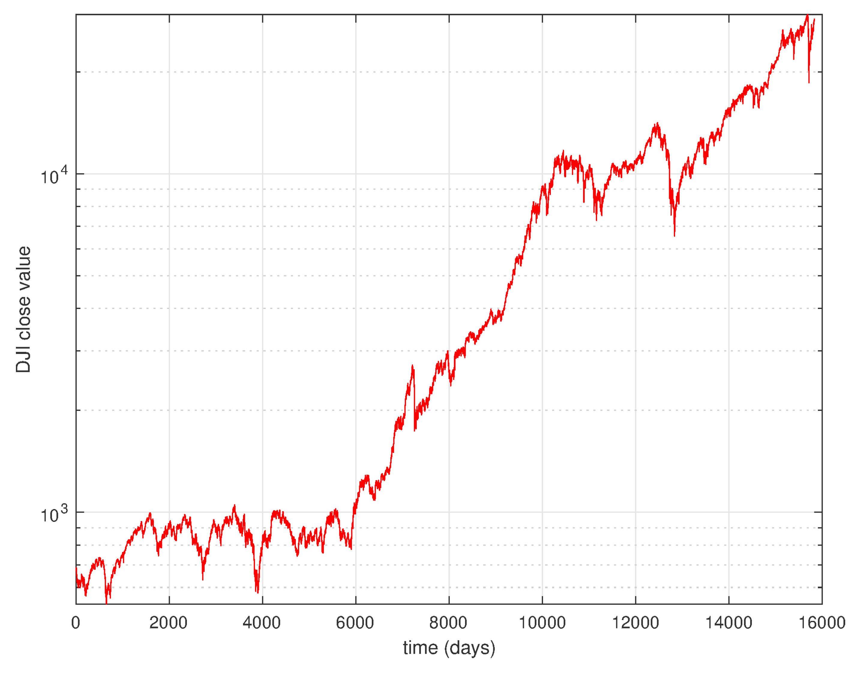
The dataset consists of the daily close values of the DJIA from 28 December 1959, up to 1 September 2020, corresponding to a time series of 15,832 days, covering approximately half a century. Each week consists of 5 working days, and some missing data due to special events were estimated by means of linear interpolation between adjacent values.
We assess the dynamics of the DJIA by comparing its values for a given time window of days. Therefore, the ith vector of DJIA values consists of , where days “1” and “” denote the start and end time instants in the time window. Hereafter, for simplicity, we consider consecutive disjoint time windows, and a number of experiments with having values multiples of 5 days. Therefore, the total number of time windows (and vectors) is , where denotes the floor function, which gives as the output the greatest integer less than or equal to the input value.
2.2. Distances
The DJIA dynamics is studied indirectly through the MDS by comparing the vectors , , , and analyzing the properties of the resulting plot in the perspective of entropy and fractal dimension. This approach requires the definition of an appropriate distance [62]. A function on a set is a “distance” when, for the items , it satisfies the conditions (i) (non-negativity), (ii) (identity of indiscernibles) if and only if , (iii) (symmetry), and (iv) (triangle inequality). If the three conditions are followed, then the function is a “metric” and together with yields a “metric space”. Obviously, these conditions still allow a considerable freedom, and we find in the literature a plethora of possible metrics each with its own pros and cons. In practice, users adopt one or more distances if they capture adequately the characteristics of the items under assessment. Therefore, we start by considering a test bench of 10 distinct indices, namely the Manhattan, Euclidean, Tchebychev, Lorentzian, Sørensen, Canberra, Clark, divergence, angular, and Jaccard distances (denoted as {Ma, Eu, Tc, Lo, So, Ca, Cl, Dv, Ac, Ja}), given by [63]:
where and , , are the ith and jth vectors of the DJIA time series, each of dimension . The Manhattan, Euclidean, and Tchebychev distances are particular cases of the Minkowski distance , namely for , and , respectively. The Lorentzian distance applies the natural logarithm to the absolute difference with 1 added to guarantee the non-negativity property and to eschew the log of zero. We find in the literature several distinct versions of the Sørensen distance, eventually with other names, and representing a statistic used for comparing the similarity between two samples. The Canberra and Clark distances are weighted versions of the Manhattan and Euclidean distances. These expressions replace by and are sensitive to small changes near zero. The angular cosine distance follows the cosine similarity that comes from the inner product of two vectors, . The angular cosine distance gives the angle between the vectors and . The Jaccard distance is the ratio of the size of the symmetric difference to the union of two sets.
2.3. The MDS Loci
Once having defined the metric for comparing the vectors, the MDS requires the construction of a matrix of item-to-item distances. In our case, “item” corresponds to a -dim vectors. Therefore, the square matrix is symmetric, with the main diagonal of zeros and dimension equal to the number of items. The MDS computational algorithm tries to plot the items in a low-dimensional space so that users can easily analyze possible relationships that are difficult to unravel in a high number of dimensions. In other words, the MDS performs a dimension reduction and plots items in a dimensional space, by estimating a matrix , corresponding to the p-dim items , so that the distances, , mimic the original ones, .
The classical MDS can perform the optimization procedure based on a variety of loss functions, often called “strain”, that are a form of minimizing the residual sum of squares. The metric MDS generalizes the optimization procedure called “stress”, , such as:
or:
where , .
The generalized MDS is an extension of metric formulation, so that the target space is an arbitrary smooth non-Euclidean space.
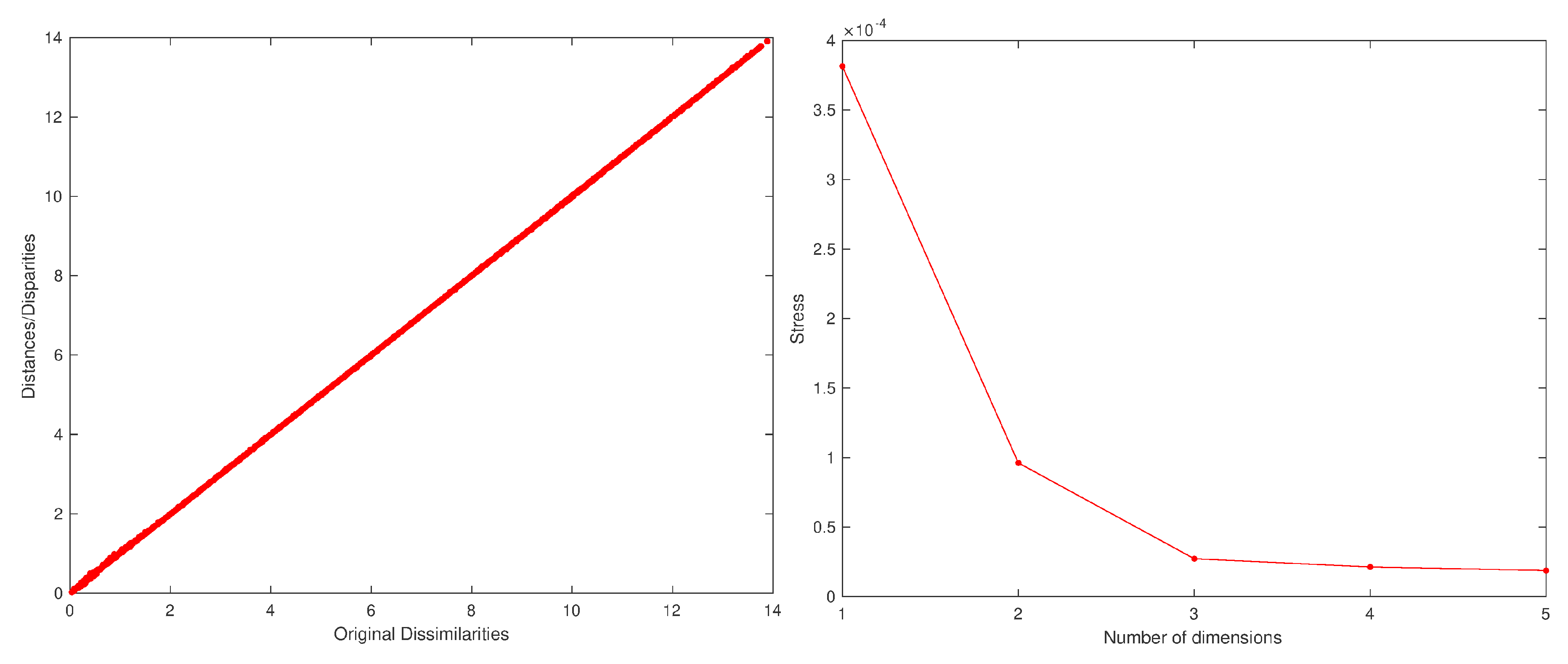
Once having obtained the MDS estimate coordinates of the objects , the user can decide the dimension p for visualization. Usually, the values and are selected since they allow a direct representation. Moreover, the quality of the MDS approximation can be assessed by means of the Sheppard and stress charts. The Sheppard diagram plots vs. . If the points follow a straight/curved line, this means a linear/non-linear relationship, but in both cases, the smaller the scatter, the better the approximation is. A second assessment tool consists of the plot of vs. p. Usually, the curve is monotonic decreasing with a large diminishing at first and a slow variation afterwards.
Since the MDS locus results from relative information (i.e., the distances), the coordinates usually do not have some physical meaning, and the user can rotate, shift, or magnify the representation to have a better view. Moreover, distinct distances lead to different plots that are correct from the mathematical and computational viewpoints, but that reflect distinct characteristics of the dataset. Therefore, it is up to the user to choose one or more distances that better highlight the aspects of the dataset under study.
Often, it is recommended to pre-process the data before calculating the distances in order to reduce the sensitivity to some details such as different units or a high variation of numerical values. In the case of the DJIA, two data pre-processing schemes (also called normalizing, or data transformation), and , are considered: (i) subtracting the arithmetic average and dividing by the standard variation, that is by calculating , where and , and (ii) by applying a logarithm so that . The linear transformation is often adopted in statistics and signal processing [64,65,66,67,68], while the non-linear transformation can be adopted with signals revealing an exponential-like evolution [69,70,71,72,73]. Of course, other data transformations could be envisaged, but these two are commonly adopted. Therefore, the main question concerning this issue is to understand to what extend the pre-processing influences the final results.
2.3.1. Data Pre-Processing Using
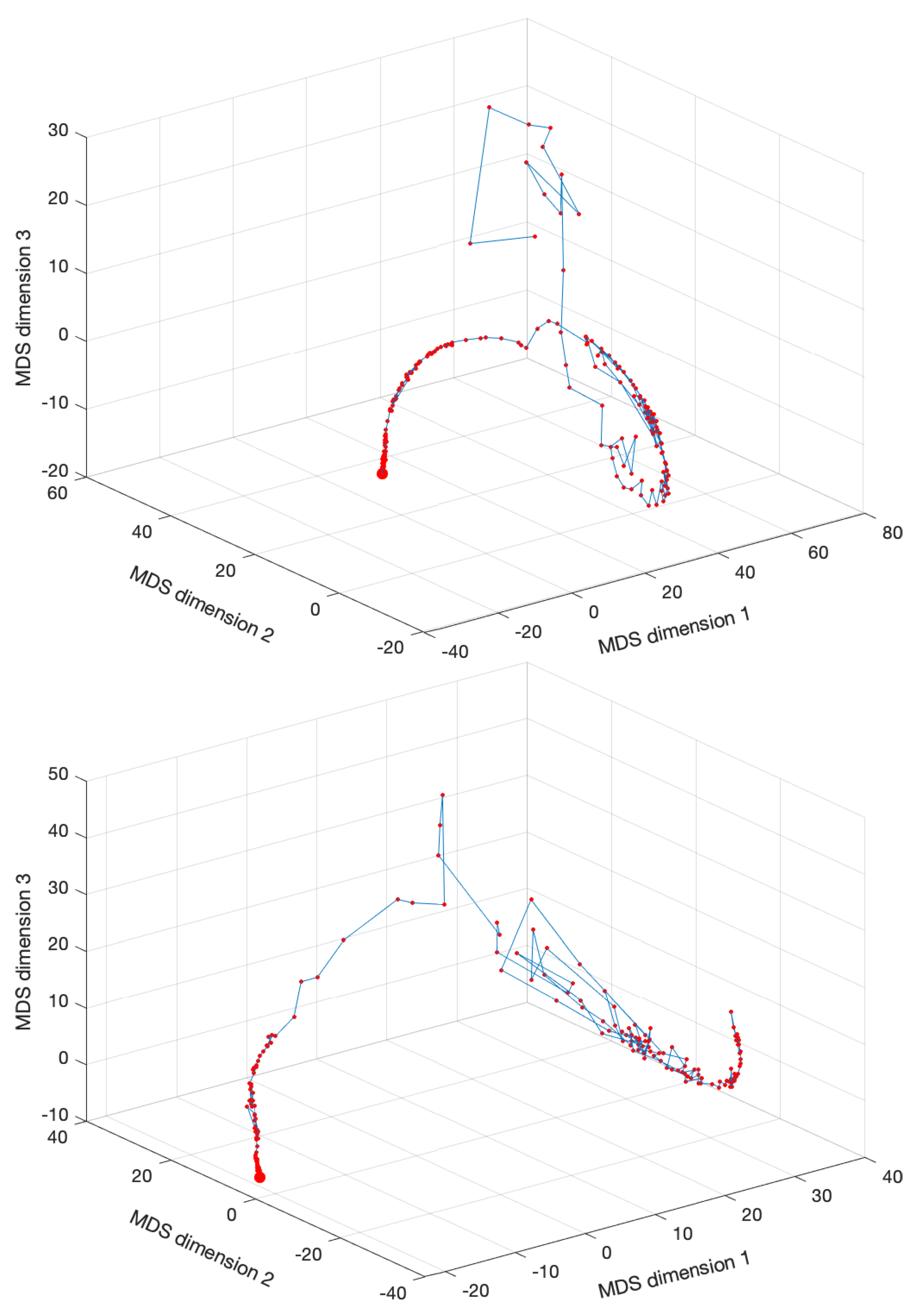
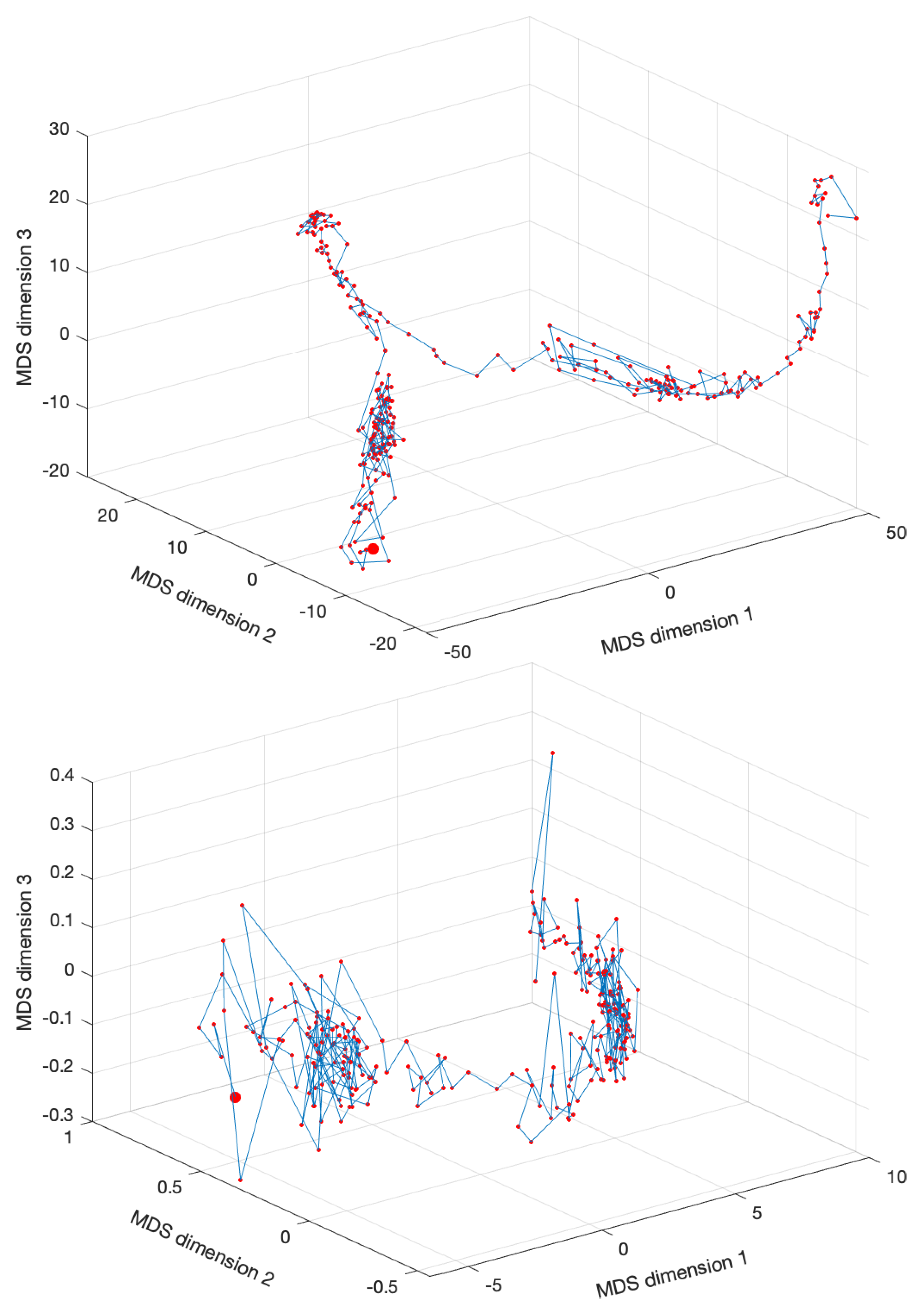
Figure 3 shows the MDS locus for and days, with pre-processing and using the Lorentzian and Canberra distances, and . The larger circle represents the first vector, and the lines connect two consecutive dots (representing the vectors from two consecutive time windows). The lines are included simply for auxiliary purposes and for highlighting the discontinuities. The MATLAB nonclassical multidimensional scaling algorithm mdscale and the Sammon’s nonlinear mapping criterion sammon were used. Figure 4 illustrates the corresponding Sheppard and stress diagrams for the Canberra distance (1f). For the sake of parsimony, the other charts are not represented.
We verify that the MDS loci exhibit segments where we have an almost continuous evolution and others with strong discontinuities. The first segments portray relatively smooth dynamics, while the second ones represent dramatic variations, in the perspective of the adopted distance and visualization technique. These dynamical effects are not read in the same way as with the standard time representations. Moreover, their visualization varies according to the type of distance adopted to construct the matrix . This should be expected, since it is well known that each distance highlights a specific set of properties embedded in the original time series and that the selection of one of more distances has to be performed on a case-by-case basis, before deciding those more adapted to the dataset.
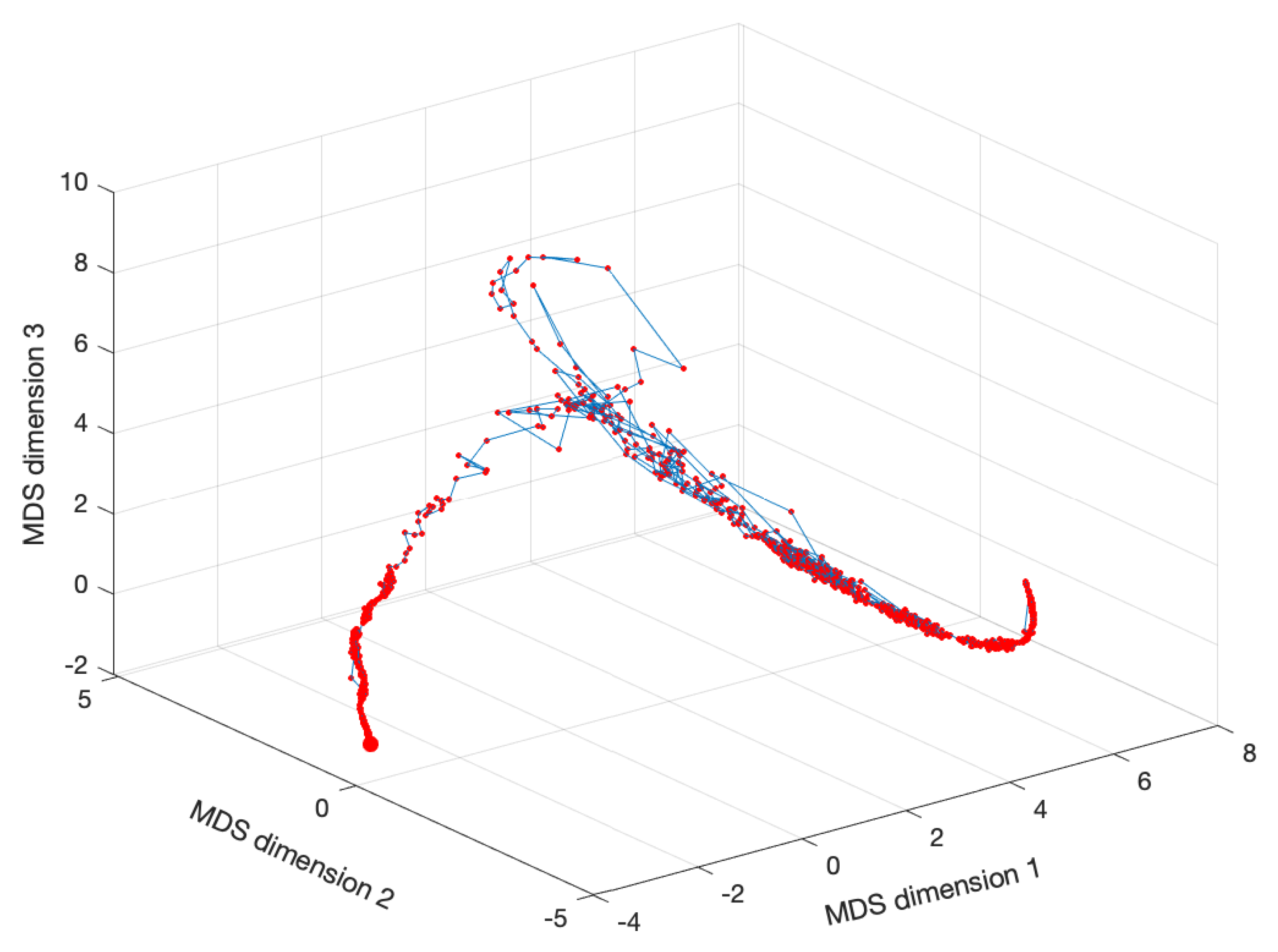
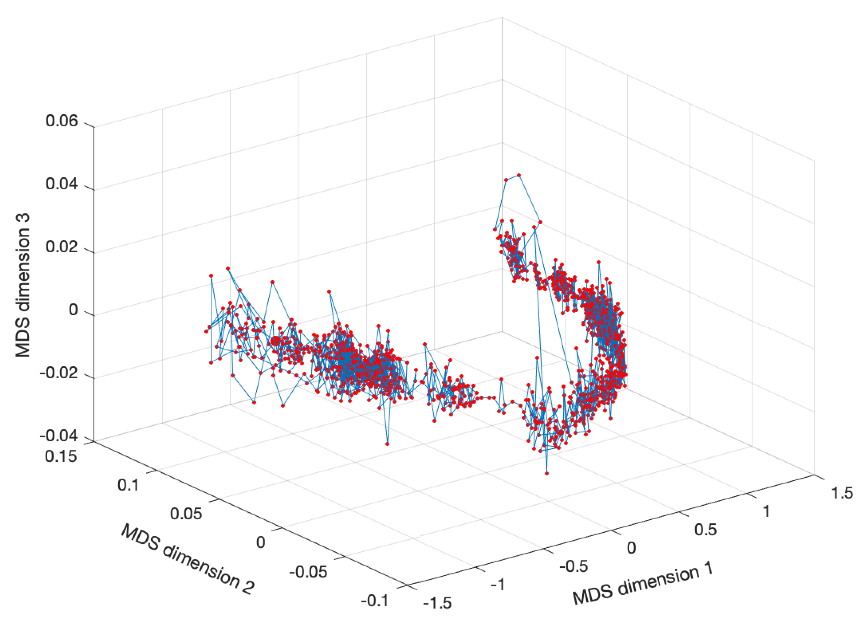
Another relevant topic is the effect of the time window on the results. In other words, we can ask how the dimension of the vector , , capturing the DJIA time dynamics, influences the MDS representation. For example, Figure 5 shows the MDS locus for , days (), and the Canberra distance (1e).
2.3.2. Data Pre-Processing Using
Figure 6 shows the MDS locus for and days, with pre-processing and using the Lorentzian and Canberra distances, and . Figure 7 depicts the Sheppard and stress diagrams for the Canberra distance (1f).
We can also check the effect of the time window . Figure 8 shows the MDS locus for , days (), and the Canberra distance (1e) revealing, again, a slight diminishing of the volatility.
As in the previous sub-section, we observe that the MDS plots reveal some segments almost with a continuous evolution and some with discontinuities. Furthermore, as before, increasing reduces the volatility in the MDS representations. These results, with regions of smooth variation, interspersed with abrupt changes, were already noticed since they reflect relativistic time effects [74,75]. Such dynamics was interpreted as a portrait of the fundamental non-smooth nature of the flow of the time variable underlying the DJIA evolution. Nonetheless, we are still far from a comprehensive understanding of the MDS loci, and we need to design additional tools to extract additional conclusions.
3. Fractal, Entropy, and Fractional Analysis
We consider the fractal dimension and entropy measures for analyzing the 3-dim portraits produced by the MDS.
The fractal dimension, , characterizes the fractal pattern of a given object by quantifying the ratio of the change in detail to the change in scale. Several types of fractal dimension can be found in the literature. In our case, is calculated by means of the box counting method as the exponent of a power law , where a is a parameter that depends on the shape and size of the object, and N and stand for the number of boxes required to capture the object and the size (or scale) of the box, respectively. Therefore, can be estimated as:
The entropy of a random variable is the average level of “information” of the corresponding probability distribution. The key cornerstone of the Shannon theory consists of the information content, which for an event having probability of occurrence , is given by:
For a 3-dim random variable with probability distribution , the Shannon entropy, , is given by:
where is the information for the event with probability .
The concept of entropy can be generalized in the scope of fractional calculus [76,77,78,79,80,81,82,83,84,85,86]. This approach gives more freedom to adapt the entropy measure to the phenomenon under study by adjusting the fractional order. The information and entropy of order are given by [77,87]:
where and represent the gamma and digamma functions.
The parameter gives an extra degree of freedom to adapt the sensitivity of the entropy calculation of each specific data series.
In an algorithmic perspective, these measures require the adoption of some grid (or box) for capturing and counting the objects, the main difference being that the fractal dimension just considers a Boolean perspective of “1” and “0”, that is the box is either full or empty, while the entropy considers the number of counts in each box.
In the follow-up, a 3-dim grid defined between the minimum and maximum values obtained for each axis of the MDS locus is considered. For the fractal dimension, we obtain by the slope of versus for 10 decreasing values of the box sizes. In the case of the entropy, we calculate when adopting 20 bins for each MDS axis. The auxiliary lines connecting the object (i.e., the points) are not considered for the calculations.
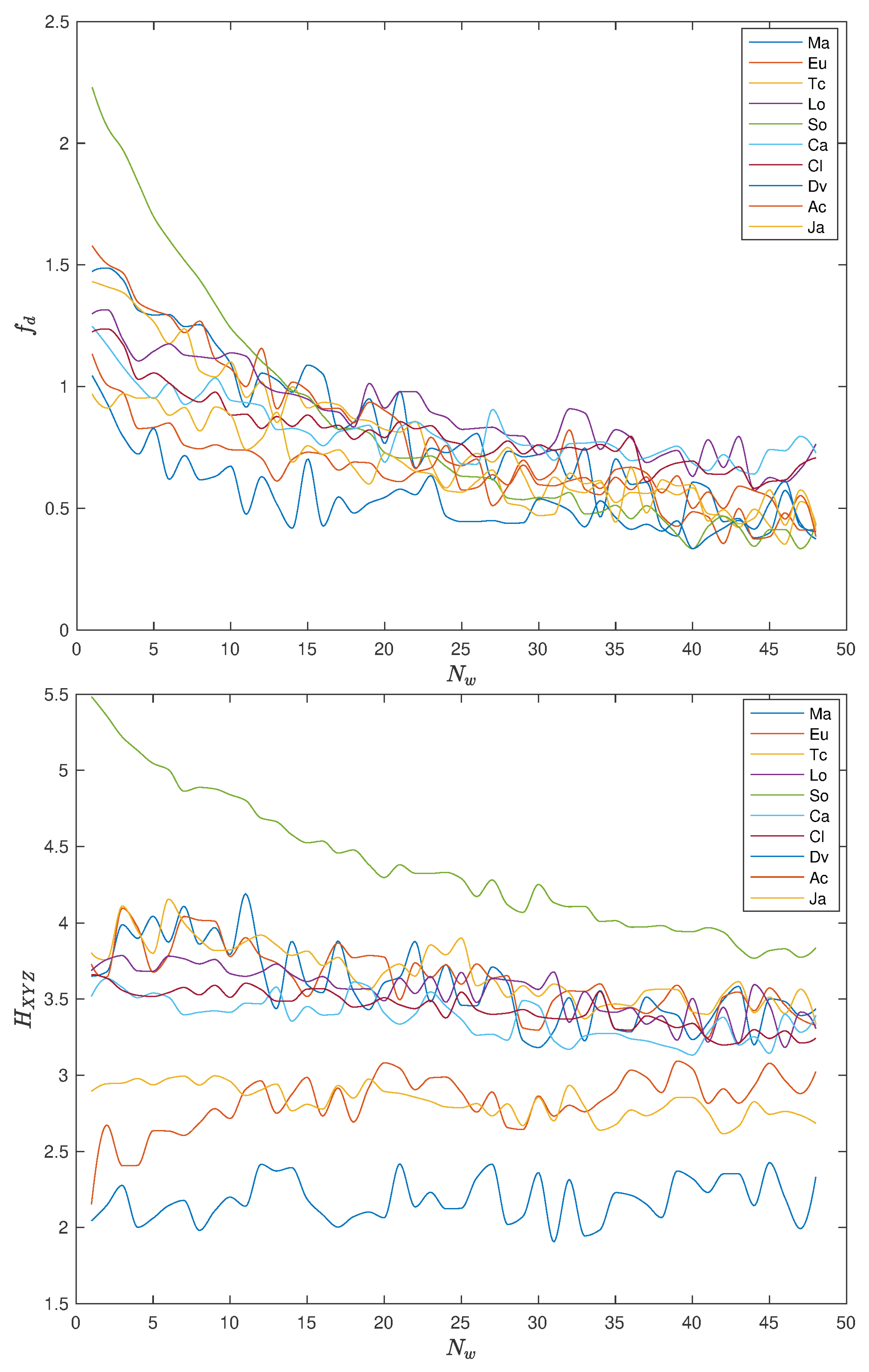
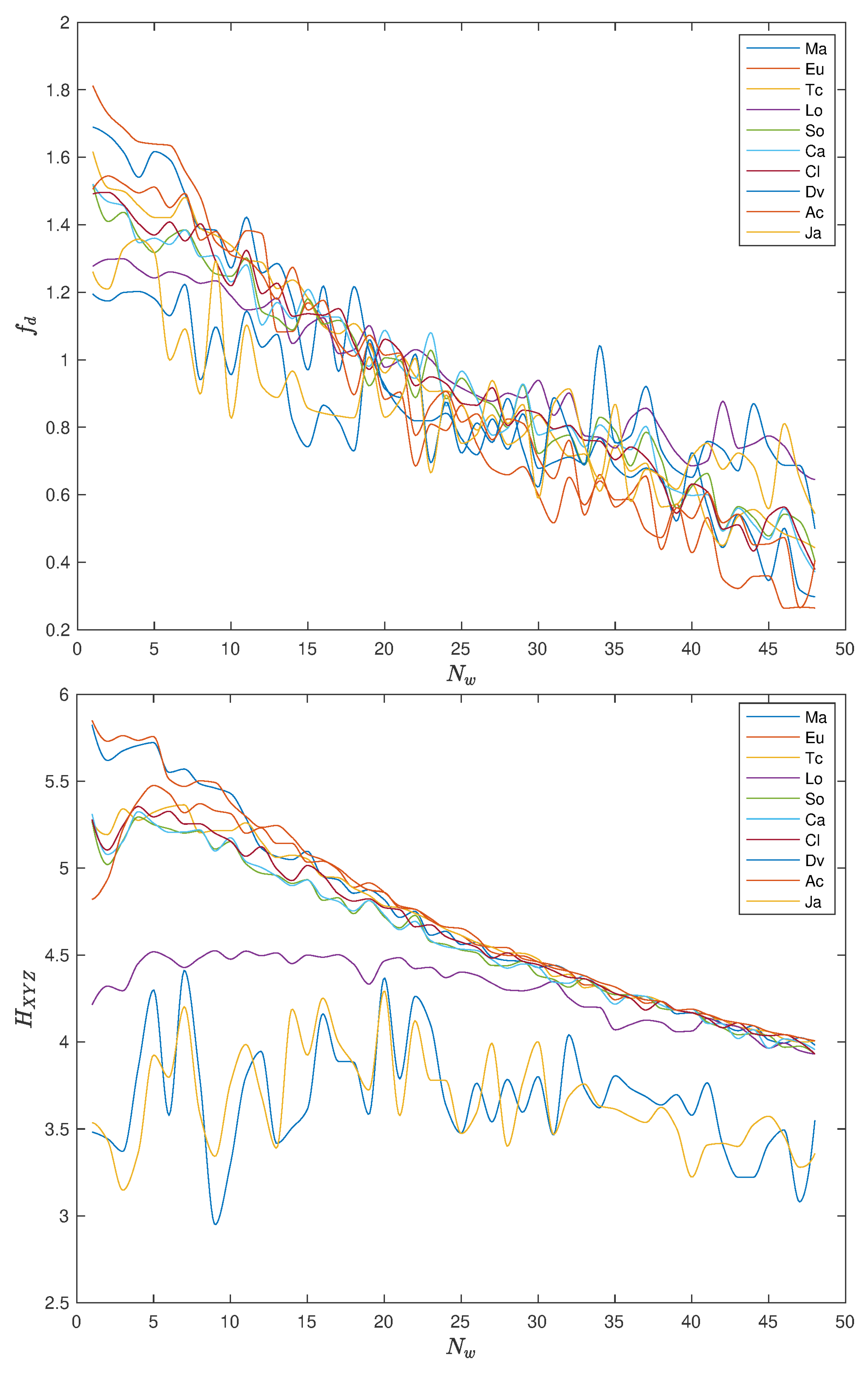
Figure 9 and Figure 10 show the variation of and with , with pre-processing and , respectively, when using the distances (1a)–(1j). For , we have correspondingly MDS with () points.
We note some “noise”, but that should be expected due to the numerical nature of the experiments. In general, the two indices decrease with , revealing, again, the “low pass filtering” effect of the dimension of the time window. We note a considerable difference of the values of and for small values of , but a stabilization and some convergence to closer values when increases.
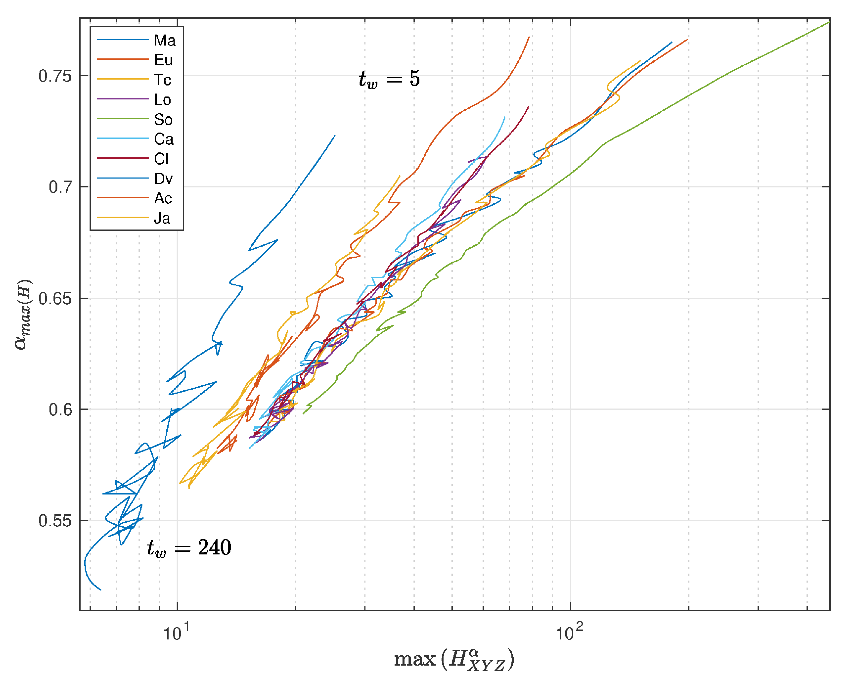
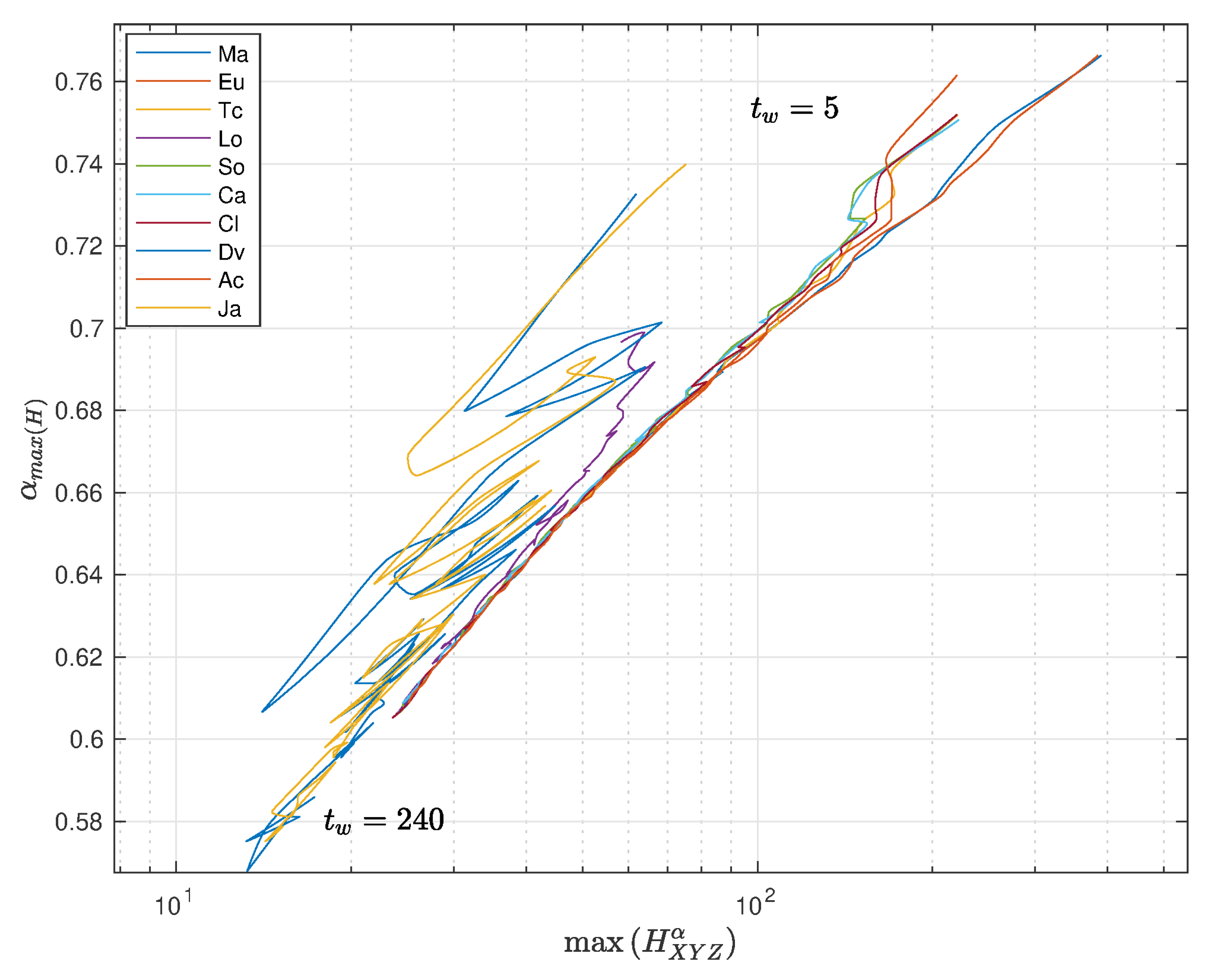
In the case of the fractional entropy, , we can tune the value of to achieve a maximum sensitivity. In other words, we can select the value to obtain . Figure 11 and Figure 12 depict vs. with , with pre-processing and , respectively, and using the distances (1a)–(1j).
We verify a strong correlation between the entropy and the value of the fractional order. Furthermore, we note that and for and , respectively, far from integer values and clearly representative of fractional dynamics. For small time windows, each distance has a distinct behavior, but when the time window increases, all distances converge to almost similar points of , both for and . Obviously, with larger time windows, we have a smaller number of points in the MDS locus, and that influences the result. The convergence towards a common behavior for all distances is observed after the first values of . This means that we are unraveling the fractional dynamics, that is a characteristic of long-range memory effects embedded in the time series.
For the pre-processing , the divergence distance produces a slightly separated plot to the left, while for , we see that position is occupied the divergence and Jaccard distances, but with a fuzzier behavior. As before, we note that the type of pre-processing does not yield any significant modification of the global conclusions.
4. Conclusions
Commonly, time is viewed as a continuous and linear flow so that any perturbation, such as noise and volatility, is automatically assigned to the variable under analysis. In other words, since we are entities immersed in the time flow, apparently, we are incapable of distinguishing between perturbations in the time and the measured variable. This paper explored an alternative strategy of reading the relationship between the variables. For that purpose, the DJIA, from 28 December 1959, up to 1 September 2020, was adopted as the vehicle for the numerical experiments. This dataset corresponds to a human-made phenomenon, and therefore, any conjecture about the nature of time is independent of the presently accepted conceptions about its flux. In the proposed approach, the time series was organized into vectors corresponding to specified time windows. Those vectors were then compared by means of a panoply of distances and the resulting information plotted in a three-dimensional space by means of MDS. Indeed, the MDS representation corresponds to a “customized projection” of high-dimensional data into a low-dimensional space. Loosely speaking, we can say “customized projection” since we do not pose any a priori requirements, the algorithm merely being based on the idea of minimizing the difference between the original measurements and the replicated (approximated) value. Therefore, the MDS does not automatically guarantee the success of such a “projection”, but the quality results were assessed by the stress and Shepard diagrams. In the case of the DJIA and the adopted distances, the good quality of the MDS technique was confirmed.
The MDS loci have distinct shapes, according to the type of distance adopted to compare vectors. Therefore, additional tools were necessary to highlight the main characteristics of these representations where time is no longer the explicit variable. For that purpose, several mathematical tools were considered, namely the Shannon entropy and fractal dimension. In all cases, we observed some variability with the time window, which occurs naturally due to the numerical treatment of this type of data. The Shannon entropy and fractal dimension exhibited the same type of behavior, with a progressive variation with the time window and a stabilization toward a common value for large . While these results can be read merely as the effect of a low pass filtering provided by the large time window, we can also foresee that another property inherent to the DJIA is their origin.
The fractional entropy was brought up to further analyze the MDS locus. This tool allows a better sensitivity to the dataset than the Shannon entropy, since users can tune the calculations by means of the fractional order. In the case of the DJIA, the tuning of for achieving the maximum entropy revealed not only that such values are independent of the distance, but also that we clearly have orders far from integer values, characteristic of fractional dynamics with non-local effects.
Some concepts are debatable and do not follow the standard orthodoxy, but the set of experiments with an artificial time series allows thinking outside the box and provides a strategy for exploring the texture of time in the perspective of entropy and fractional calculus.
Funding
This research received no external funding.
Conflicts of Interest
The author declares no conflict of interest.
References
- Trippi, R. Chaos & Nonlinear Dynamics in the Financial Markets; Irwin Professional Publishing Company: Burr Ridge, IL, USA, 1995. [Google Scholar]
- Vialar, T. Complex and Chaotic Nonlinear Dynamics: Advances in Economics and Finance, Mathematics and Statistics; Springer: Berlin/Heidelberg, Germany, 2009. [Google Scholar]
- Bischi, G.I.; Chiarella, C.; Gardini, L. (Eds.) Nonlinear Dynamics in Economics, Finance and the Social Sciences; Springer: Berlin/Heidelberg, Germany, 2010. [Google Scholar]
- Meyers, R.A. (Ed.) Complex Systems in Finance and Econometrics; Springer: New York, NY, USA, 2010. [Google Scholar]
- Machado, J.A.T. Calculation of Fractional Derivatives of Noisy Data with Genetic Algorithms. Nonlinear Dyn. 2009, 57, 253–260. [Google Scholar] [CrossRef] [Green Version]
- Duarte, F.B.; Machado, J.A.T.; Duarte, G.M. Dynamics of the Dow Jones and the NASDAQ Stock Indexes. Nonlinear Dyn. 2010, 61, 691–705. [Google Scholar] [CrossRef] [Green Version]
- Machado, J.T.; Duarte, F.B.; Duarte, G.M. Analysis of stock market indices through multidimensional scaling. Commun. Nonlinear Sci. Numer. Simul. 2011, 16, 4610–4618. [Google Scholar] [CrossRef] [Green Version]
- Machado, J.A.T.; Duarte, G.M.; Duarte, F.B. Analysis of Financial Data Series Using Fractional Fourier Transform and Multidimensional Scaling. Nonlinear Dyn. 2011, 65, 235–245. [Google Scholar] [CrossRef] [Green Version]
- Machado, J.A.T.; Duarte, G.M.; Duarte, F.B. Identifying Economic Periods and Crisis with the Multidimensional Scaling. Nonlinear Dyn. 2011, 63, 611–622. [Google Scholar] [CrossRef] [Green Version]
- Machado, J.T.; Duarte, F.B.; Duarte, G.M. Analysis of Financial Indices by Means of The Windowed Fourier Transform. Signal Image Video Process. 2012, 6, 487–494. [Google Scholar] [CrossRef] [Green Version]
- Machado, J.T.; Duarte, G.M.; Duarte, F.B. Analysis of stock market indices with multidimensional scaling and wavelets. Math. Probl. Eng. 2012, 2012, 14. [Google Scholar]
- Machado, J.A.T.; Duarte, G.M.; Duarte, F.B. Fractional dynamics in financial indexes. Int. J. Bifurc. Chaos 2012, 22, 1250249. [Google Scholar] [CrossRef] [Green Version]
- Machado, J.T.; Duarte, F.B.; Duarte, G.M. Power Law Analysis of Financial Index Dynamics. Discret. Dyn. Nat. Soc. 2012, 2012, 12. [Google Scholar]
- Da Silva, S.; Matsushita, R.; Gleria, I.; Figueiredo, A.; Rathie, P. International finance, Lévy distributions, and the econophysics of exchange rates. Commun. Nonlinear Sci. Numer. Simul. 2005, 10, 355–466. [Google Scholar] [CrossRef] [Green Version]
- Chen, W.C. Nonlinear dynamics and chaos in a fractional-order financial system. Chaos Solitons Fractals 2008, 36, 1305–1314. [Google Scholar] [CrossRef]
- Piqueira, J.R.C.; Mortoza, L.P.D. Complexity analysis research of financial and economic system under the condition of three parameters’ change circumstances. Commun. Nonlinear Sci. Numer. Simul. 2012, 17, 1690–1695. [Google Scholar] [CrossRef]
- Ma, J.; Bangura, H.I. Complexity analysis research of financial and economic system under the condition of three parameters’ change circumstances. Nonlinear Dyn. 2012, 70, 2313–2326. [Google Scholar] [CrossRef]
- Ngounda, E.; Patidar, K.C.; Pindza, E. Contour integral method for European options with jumps. Commun. Nonlinear Sci. Numer. Simul. 2013, 18, 478–492. [Google Scholar] [CrossRef] [Green Version]
- Horwich, P. Asymmetries in Time: Problems in the Philosophy of Science; The MIT Press: Cambridge, MA, USA, 1987. [Google Scholar]
- Reichenbach, H. The Direction of Time; University of California Press: New York, NY, USA, 1991. [Google Scholar]
- Dainton, B. Time and Space, 2nd ed.; Acumen Publishing, Limited: Chesham, UK, 2001. [Google Scholar]
- Callender, C. (Ed.) The Oxford Handbook of Philosophy of Time; Oxford University Press: New York, NY, USA, 2011. [Google Scholar]
- Torgerson, W. Theory and Methods of Scaling; Wiley: New York, NY, USA, 1958. [Google Scholar]
- Shepard, R.N. The analysis of proximities: Multidimensional scaling with an unknown distance function. Psychometrika 1962, 27, 219–246. [Google Scholar] [CrossRef]
- Kruskal, J. Multidimensional scaling by optimizing goodness of fit to a nonmetric hypothesis. Psychometrika 1964, 29, 1–27. [Google Scholar] [CrossRef]
- Sammon, J. A nonlinear mapping for data structure analysis. IEEE Trans. Comput. 1969, 18, 401–409. [Google Scholar] [CrossRef]
- Kruskal, J.B.; Wish, M. Multidimensional Scaling; Sage Publications: Newbury Park, CA, USA, 1978. [Google Scholar]
- Borg, I.; Groenen, P.J. Modern Multidimensional Scaling-Theory and Applications; Springer: New York, NY, USA, 2005. [Google Scholar]
- Saeed, N.; Nam, H.; Imtiaz, M.; Saqib, D.B.M. A Survey on Multidimensional Scaling. ACM Comput. Surv. CSUR 2018, 51, 47. [Google Scholar] [CrossRef] [Green Version]
- Mandelbrot, B.B.; Ness, J.W.V. The fractional Brownian motions, fractional noises and applications. SIAM Rev. 1968, 10, 422–437. [Google Scholar] [CrossRef]
- Mandelbrot, B.B. The Fractal Geometry of Nature; W. H. Freeman: New York, NY, USA, 1983. [Google Scholar]
- Berry, M.V. Diffractals. J. Phys. A Math. Gen. 1979, 12, 781–797. [Google Scholar] [CrossRef]
- Lapidus, M.L.; Fleckinger-Pellé, J. Tambour fractal: Vers une résolution de la conjecture de Weyl-Berry pour les valeurs propres du Laplacien. C. R. L’Académie Sci. Paris Sér. I Math. 1988, 306, 171–175. [Google Scholar]
- Schroeder, M. Fractals, Chaos, Power Laws: Minutes from an Infinite Paradise; W. H. Freeman: New York, NY, USA, 1991. [Google Scholar]
- Shannon, C.E. A mathematical theory of communication. Bell Syst. Tech. J. 1948, 27, 379–423, 623–656. [Google Scholar] [CrossRef] [Green Version]
- Khinchin, A.I. Mathematical Foundations of Information Theory; Dover: New York, NY, USA, 1957. [Google Scholar]
- Jaynes, E.T. Information Theory and Statistical Mechanics. Phys. Rev. 1957, 106, 620–630. [Google Scholar] [CrossRef]
- Rényi, A. On measures of information and entropy. In Proceedings of the fourth Berkeley Symposium on Mathematics, Statistics and Probability, Volume 1: Contributions to the Theory of Statistics, Berkeley, CA, USA, 20 June–30 July 1960; University of California Press: Berkeley, CA, USA, 1961; pp. 547–561. Available online: https://projecteuclid.org/euclid.bsmsp/1200512181 (accessed on 4 September 2020).
- Brillouin, L. Science and Information Theory; Academic Press: London, UK, 1962. [Google Scholar]
- Lin, J. Divergence measures based on the Shannon entropy. IEEE Trans. Inf. Theory 1991, 37, 145–151. [Google Scholar] [CrossRef] [Green Version]
- Beck, C. Generalised information and entropy measures in physics. Contemp. Phys. 2009, 50, 495–510. [Google Scholar] [CrossRef]
- Gray, R.M. Entropy and Information Theory; Springer: New York, NY, USA, 2011. [Google Scholar]
- Oldham, K.; Spanier, J. The Fractional Calculus: Theory and Application of Differentiation and Integration to Arbitrary Order; Academic Press: New York, NY, USA, 1974. [Google Scholar]
- Samko, S.; Kilbas, A.; Marichev, O. Fractional Integrals and Derivatives: Theory and Applications; Gordon and Breach Science Publishers: Amsterdam, The Netherlands, 1993. [Google Scholar]
- Miller, K.; Ross, B. An Introduction to the Fractional Calculus and Fractional Differential Equations; John Wiley and Sons: New York, NY, USA, 1993. [Google Scholar]
- Kilbas, A.; Srivastava, H.; Trujillo, J. Volume 204, North-Holland Mathematics Studies. In Theory and Applications of Fractional Differential Equations; Elsevier: Amsterdam, The Netherlands, 2006. [Google Scholar]
- Kochubei, A.; Luchko, Y. (Eds.) Volume 1, De Gruyter Reference. In Handbook of Fractional Calculus with Applications: Basic Theory; De Gruyter: Berlin, Germany, 2019. [Google Scholar]
- Kochubei, A.; Luchko, Y. (Eds.) Volume 2, De Gruyter Reference. In Handbook of Fractional Calculus with Applications: Fractional Differential Equations; De Gruyter: Berlin, Germany, 2019. [Google Scholar]
- Westerlund, S.; Ekstam, L. Capacitor theory. IEEE Trans. Dielectr. Electr. Insul. 1994, 1, 826–839. [Google Scholar] [CrossRef]
- Grigolini, P.; Aquino, G.; Bologna, M.; Luković, M.; West, B.J. A theory of 1/f noise in human cognition. Phys. A Stat. Mech. Its Appl. 2009, 388, 4192–4204. [Google Scholar] [CrossRef]
- West, B.J.; Grigolini, P. Complex Webs: Anticipating the Improbable; Cambridge University Press: New York, NY, USA, 2010. [Google Scholar]
- Tarasov, V. Fractional Dynamics: Applications of Fractional Calculus to Dynamics of Particles, Fields and Media; Springer: New York, NY, USA, 2010. [Google Scholar]
- Mainardi, F. Fractional Calculus and Waves in Linear Viscoelasticity: An Introduction to Mathematical Models; Imperial College Press: London, UK, 2010. [Google Scholar]
- Ortigueira, M.D. Fractional Calculus for Scientists and Engineers; Lecture Notes in Electrical Engineering; Springer: Dordrecht, The Netherlands, 2011. [Google Scholar]
- West, B.J. Fractional Calculus View of Complexity: Tomorrow’s Science; CRC Press: Boca Raton, FL, USA, 2015. [Google Scholar]
- Tarasov, V.E. (Ed.) Volume 4, De Gruyter Reference. In Handbook of Fractional Calculus with Applications: Applications in Physics, Part A; De Gruyter: Berlin, Germany, 2019. [Google Scholar]
- Tarasov, V.E. (Ed.) Volume 5, De Gruyter Reference. In Handbook of Fractional Calculus with Applications: Applications in Physics, Part B; De Gruyter: Berlin, Germany, 2019. [Google Scholar]
- Machado, J.A.T.; Mata, M.E. A multidimensional scaling perspective of Rostow’s forecasts with the track-record (1960s–2011) of pioneers and latecomers. In Dynamical Systems: Theory, Proceedings of the 12th International Conference on Dynamical Systems—Theory and Applications; Awrejcewicz, J., Kazmierczak, M., Olejnik, P., Mrozowski, J., Eds.; Łódź University of Technology: Łódź, Poland, 2013; pp. 361–378. [Google Scholar]
- Machado, J.A.T.; Mata, M.E. Analysis of World Economic Variables Using Multidimensional Scaling. PLoS ONE 2013, 10, e0121277. [Google Scholar] [CrossRef] [Green Version]
- Tenreiro Machado, J.A.; Lopes, A.M.; Galhano, A.M. Multidimensional scaling visualization using parametric similarity indices. Entropy 2015, 17, 1775–1794. [Google Scholar] [CrossRef] [Green Version]
- Mata, M.; Machado, J. Entropy Analysis of Monetary Unions. Entropy 2017, 19, 245. [Google Scholar] [CrossRef]
- Deza, M.M.; Deza, E. Encyclopedia of Distances; Springer: Berlin/Heidelberg, Germany, 2009. [Google Scholar]
- Cha, S.H. Measures between Probability Density Functions. Int. J. Math. Model. Methods Appl. Sci. 2007, 1, 300–307. [Google Scholar]
- Papoulis, A. Signal Analysis; McGraw-Hill: New York, NY, USA, 1977. [Google Scholar]
- Oppenheim, A.V.; Schafer, R.W. Digital Signal Processing; Prentice Hall: Upper Saddle River, NJ, USA, 1989. [Google Scholar]
- Parzen, E. Modern Probability Theory and Its Applications; Wiley-Interscience: New York, NY, USA, 1992. [Google Scholar]
- Pollock, D.S.; Green, R.C.; Nguyen, T. (Eds.) Handbook of Time Series Analysis, Signal Processing, and Dynamics (Signal Processing and Its Applications); Academic Press: London, UK, 1999. [Google Scholar]
- Small, M. Applied Nonlinear Time Series Analysis: Applications in Physics, Physiology and Finance; World Scientific Publishing: Singapore, 2005. [Google Scholar]
- Keene, O.N. The log transformation is special. Stat. Med. 1995, 14, 811–819. [Google Scholar] [CrossRef] [PubMed]
- Leydesdorff, L.; Bensman, S. Classification and powerlaws: The logarithmic transformation. J. Am. Soc. Inf. Sci. Technol. 2006, 57, 1470–1486. [Google Scholar] [CrossRef] [Green Version]
- Stango, V.; Zinman, J. Exponential Growth Bias and Household Finance. J. Financ. 2009, 64, 2807–2849. [Google Scholar] [CrossRef]
- Feng, C.; Wang, H.; Lu, N.; Chen, T.; He, H.; Lu, Y.; Tu, X.M. Log-transformation and its implications for data analysis. Shanghai Arch. Psychiatry 2014, 26, 105–109. [Google Scholar] [CrossRef] [PubMed]
- Lopes, A.; Machado, J.T.; Galhano, A. Empirical Laws and Foreseeing the Future of Technological Progress. Entropy 2016, 18, 217. [Google Scholar] [CrossRef] [Green Version]
- Machado, J.A.T. Complex Dynamics of Financial Indices. Nonlinear Dyn. 2013, 74, 287–296. [Google Scholar] [CrossRef] [Green Version]
- Machado, J.A.T. Relativistic Time Effects in Financial Dynamics. Nonlinear Dyn. 2014, 75, 735–744. [Google Scholar] [CrossRef] [Green Version]
- Ubriaco, M.R. Entropies based on fractional calculus. Phys. Lett. A 2009, 373, 2516–2519. [Google Scholar] [CrossRef] [Green Version]
- Machado, J.A.T. Fractional Order Generalized Information. Entropy 2014, 16, 2350–2361. [Google Scholar] [CrossRef] [Green Version]
- Karci, A. Fractional order entropy: New perspectives. Optik 2016, 127, 9172–9177. [Google Scholar] [CrossRef]
- Bagci, G.B. The third law of thermodynamics and the fractional entropies. Phys. Lett. A 2016, 380, 2615–2618. [Google Scholar] [CrossRef]
- Xu, J.; Dang, C. A novel fractional moments-based maximum entropy method for high-dimensional reliability analysis. Appl. Math. Model. 2019, 75, 749–768. [Google Scholar] [CrossRef]
- Xu, M.; Shang, P.; Qi, Y.; Zhang, S. Multiscale fractional order generalized information of financial time series based on similarity distribution entropy. Chaos Interdiscip. J. Nonlinear Sci. 2019, 29, 053108. [Google Scholar] [CrossRef] [PubMed]
- Machado, J.A.T.; Lopes, A.M. Fractional Rényi entropy. Eur. Phys. J. Plus 2019, 134. [Google Scholar] [CrossRef]
- Ferreira, R.A.C.; Machado, J.T. An Entropy Formulation Based on the Generalized Liouville Fractional Derivative. Entropy 2019, 21, 638. [Google Scholar] [CrossRef] [Green Version]
- Matouk, A. Complex dynamics in susceptible-infected models for COVID-19 with multi-drug resistance. Chaos Solitons Fractals 2020, 140, 110257. [Google Scholar] [CrossRef]
- Matouk, A.; Khan, I. Complex dynamics and control of a novel physical model using nonlocal fractional differential operator with singular kernel. J. Adv. Res. 2020, 24, 463–474. [Google Scholar] [CrossRef]
- Matouk, A.E. (Ed.) Advanced Applications of Fractional Differential Operators to Science and Technology; IGI Global: Hershey, PA, USA, 2020. [Google Scholar] [CrossRef]
- Valério, D.; Trujillo, J.J.; Rivero, M.; Machado, J.T.; Baleanu, D. Fractional Calculus: A Survey of Useful Formulas. Eur. Phys. J. Spec. Top. 2013, 222, 1827–1846. [Google Scholar] [CrossRef]
Figure 1.
Daily close values of the DJIA from 28 December 1959, up to 1 September 2020.

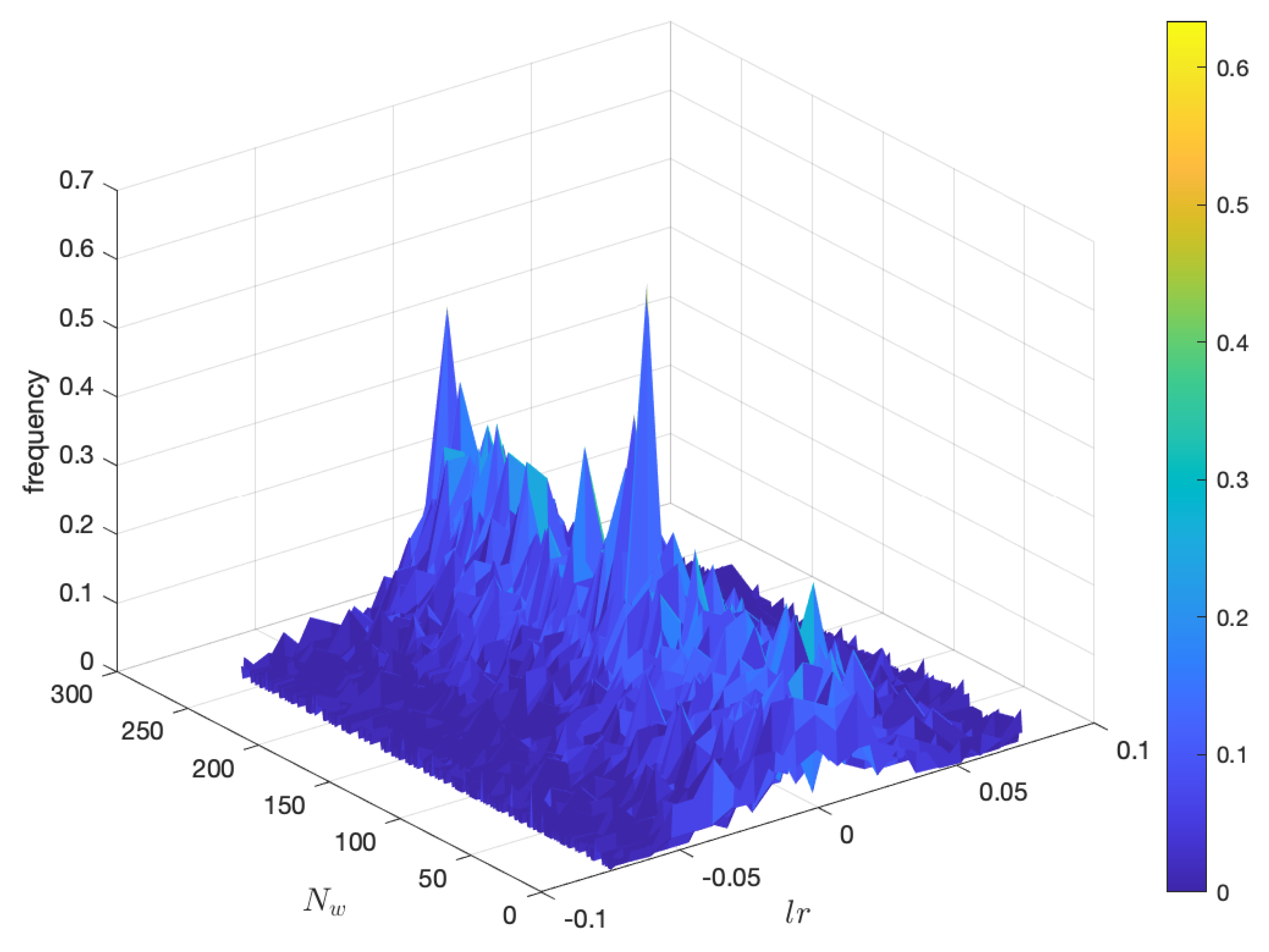
Figure 2.
Histogram of the logarithm of the returns of the DJIA from 28 December 1959, up to 1 September 2020, for time windows of days.
Figure 2.
Histogram of the logarithm of the returns of the DJIA from 28 December 1959, up to 1 September 2020, for time windows of days.

Figure 3.
The multidimensional scaling (MDS) locus, , of the DJIA dataset for and days (), with pre-processing and using the Lorentzian (1d) and Canberra (1f) distances.
Figure 3.
The multidimensional scaling (MDS) locus, , of the DJIA dataset for and days (), with pre-processing and using the Lorentzian (1d) and Canberra (1f) distances.

Figure 4.
The Sheppard diagram, vs. , for , and stress plot, vs. p, of the DJIA dataset with days, with pre-processing and using the Canberra distance (1f).
Figure 4.
The Sheppard diagram, vs. , for , and stress plot, vs. p, of the DJIA dataset with days, with pre-processing and using the Canberra distance (1f).

Figure 5.
The MDS locus, , of the DJIA dataset for and days (), with pre-processing and using the Canberra distance (1e).
Figure 5.
The MDS locus, , of the DJIA dataset for and days (), with pre-processing and using the Canberra distance (1e).

Figure 6.
The MDS locus, , of the DJIA dataset for and days (), with pre-processing and using the Lorentzian (1d) and Canberra (1f) distances.
Figure 6.
The MDS locus, , of the DJIA dataset for and days (), with pre-processing and using the Lorentzian (1d) and Canberra (1f) distances.

Figure 7.
The Sheppard diagram, vs. , for , and the stress plot, vs. p, of the DJIA dataset with days, with pre-processing and using the Canberra distance (1f).
Figure 7.
The Sheppard diagram, vs. , for , and the stress plot, vs. p, of the DJIA dataset with days, with pre-processing and using the Canberra distance (1f).

Figure 8.
The MDS locus, , of the DJIA dataset for and days (), with pre-processing and using the Canberra distance (1e).
Figure 8.
The MDS locus, , of the DJIA dataset for and days (), with pre-processing and using the Canberra distance (1e).

Figure 9.
Plot of fractal dimension, , and Shannon entropy, , versus (), with pre-processing and using the distances (1a)–(1j).
Figure 9.
Plot of fractal dimension, , and Shannon entropy, , versus (), with pre-processing and using the distances (1a)–(1j).

Figure 10.
Plot of fractal dimension, , and Shannon entropy, , versus (), with pre-processing and using the distances (1a)–(1j). The Manhattan, Euclidean, Tchebychev, Lorentzian, Sørensen, Canberra, Clark, divergence, angular, and Jaccard distances (denoted as {Ma, Eu, Tc, Lo, So, Ca, Cl, Dv, Ac, Ja}).

Figure 11.
Plot of versus , with , with pre-processing and using the distances (1a)–(1j).
Figure 11.
Plot of versus , with , with pre-processing and using the distances (1a)–(1j).

Figure 12.
Plot of versus , with , with pre-processing and using the distances (1a)–(1j).
Figure 12.
Plot of versus , with , with pre-processing and using the distances (1a)–(1j).

© 2020 by the author. Licensee MDPI, Basel, Switzerland. This article is an open access article distributed under the terms and conditions of the Creative Commons Attribution (CC BY) license (http://creativecommons.org/licenses/by/4.0/).
Share and Cite
MDPI and ACS Style
Machado, J.A.T. Fractal and Entropy Analysis of the Dow Jones Index Using Multidimensional Scaling. Entropy 2020, 22, 1138. https://doi.org/10.3390/e22101138
AMA Style
Machado JAT. Fractal and Entropy Analysis of the Dow Jones Index Using Multidimensional Scaling. Entropy. 2020; 22(10):1138. https://doi.org/10.3390/e22101138
Chicago/Turabian StyleMachado, José A. Tenreiro. 2020. "Fractal and Entropy Analysis of the Dow Jones Index Using Multidimensional Scaling" Entropy 22, no. 10: 1138. https://doi.org/10.3390/e22101138
Note that from the first issue of 2016, this journal uses article numbers instead of page numbers. See further details here.