


1. Introduction
Annual snowfall over the Antarctic and Greenland ice sheets holds water equivalent to ~6.5 mm of mean sea level. Therefore, small changes in snowfall, melt and discharge of ice into the ocean can be a major contributor to sea level rise (Rignot and Thomas, Reference Rignot and Thomas2002). Consequently, accurate methods for determination of ice-sheet (surface) mass balance are of key importance for understanding environmental and socio-economic consequences of sea level rise (Rignot and others, Reference Rignot2008; van den Broeke and others, Reference van den Broeke2009; Shepherd and others, Reference Shepherd2012; Golledge and others, Reference Golledge2019). Several methods for ice-sheet mass-balance estimation exist which employ gravity measurements (Wahr and others, Reference Wahr, Swenson and Velicogna2006) and altimetry (Krabill and others, Reference Krabill2004; Zwally and others, Reference Zwally2005). However, spaceborne gravimetry suffers from coarse spatial resolution (≥40 km) and altimetry methods (e.g. microwave radar and laser altimetry) rely on modeled snow density for the computation of snow water equivalent (Sandberg Sørensen and others, Reference Sandberg Sørensen2011).
Other active (Drewry and others, Reference Drewry, Turner and Rees1991; Jezek and others, Reference Jezek, Drinkwater, Crawford, Bindschadler and Kwok1993; Long and Drinkwater, Reference Long and Drinkwater1999; Nghiem and others, Reference Nghiem, Steffen, Kwok and Tsai2001; Li and others, Reference Li, Zhang and Liang2017) and passive (Jay Zwally and Fiegles, Reference Zwally and Fiegles1994; Abdalati and Steffen, Reference Abdalati and Steffen1995; Steffen and others, Reference Steffen, Nghiem, Huff and Neumann2004; Mote, Reference Mote2007) microwave remote-sensing techniques exist which employ observations at frequencies higher than L-band (1–2 GHz) to detect liquid water in snow. While these methods provide valuable insight, they are limited to binary detection of dry/wet snow due to the limited penetration depth of higher frequency microwaves in snow (Hofer and Mätzler, Reference Hofer and Mätzler1980; Mätzler and others, Reference Mätzler, Aebischer and Schanda1984). Furthermore, liquid water changes the microstructure of snowpack, which considerably influence its scattering and emission especially at higher frequencies. Therefore, snow liquid-water retrieval methods using microwave frequencies higher than L-band require empirical tuning of melt-thresholds. Limited research has been published on the retrieval of snow properties using inversion of microwave emission models (EMs) (Tedesco and others, Reference Tedesco, Kim, England, Roo and Hardy2006), yet still these studies employ higher-frequency microwaves, limited by low penetration depth especially into wet snow.
Beginning in 2014, the ‘L-band Specific Microwave Emission Model of Layered Snowpack’ (LS-MEMLS) (Schwank and others, Reference Schwank2014) was developed with the aim of using L-band brightness temperatures to retrieve snow column- and subnivean layer properties. Since then it has been theoretically (Schwank and others, Reference Schwank2015; Schwank and Naderpour, Reference Schwank and Naderpour2018) and experimentally (Lemmetyinen and others, Reference Lemmetyinen2016; Schwank and Naderpour, Reference Schwank and Naderpour2018) demonstrated that dry snow mass-density can be retrieved from inversion of the LS-MEMLS. Furthermore, a similar approach was presented in Naderpour and Schwank (Reference Naderpour and Schwank2018) demonstrating the retrieval of snow liquid water content in ‘Davos-Laret Remote Sensing Field Laboratory’ (Naderpour and others, Reference Naderpour, Schwank and Mätzler2017). In 2019, an approach was developed, as an extension of (Naderpour and Schwank, Reference Naderpour and Schwank2018), for the retrieval of snow density and wetness at a location over the ablation zone of the Greenland Ice Sheet (GrISs) using spaceborne L-band radiometry (Houtz and others, Reference Houtz, Naderpour, Schwank and Steffen2019).
An inherent limitation in spaceborne passive microwave data (brightness temperatures) is its coarse spatial resolution, especially at low microwave frequencies such as the L-band (1–2 GHz). The soil moisture and ocean salinity (SMOS) (Kerr and others, Reference Kerr2010) level 3 satellite brightness temperatures used in Houtz and others (Reference Houtz, Naderpour, Schwank and Steffen2019) has a pixel-diameter of ~25 km, and has a limited revisit time ranging between 12 and 36 h over the GrISs. It is noteworthy that ground spatial resolution of level 1 SMOS antenna brightness temperature is even coarser ranging between 30 and 50 km (Kerr and others, Reference Kerr2001). Therefore, to better understand the sensitivity of L-band brightness temperature with respect to snow melt/refreeze cycles, an L-band radiometer (ELBARA-III) was operated at the Swiss Camp research station located in the western ablation zone of the GrIS in May 2019. Air temperature was monitored, and snow in situ data were collected from several manual snow pits. Approximately 5 days of close-range (CR) L-band antenna temperatures at a single observation nadir angle as well as several sets of multi-angle measurements were collected.
This paper presents snow wetness retrieved from single-angle dual-polarization CR L-band antenna temperatures. In addition, snow wetness retrievals derived from multi-angle CR L-band antenna temperatures, adopting the same approach as used in Houtz and others (Reference Houtz, Naderpour, Schwank and Steffen2019), are compared with snow wetness retrieved from single-angle CR L-band measurements. Furthermore, we compare CR antenna temperatures measured with the ELBARA-III L-band radiometer against SMOS brightness temperatures.
2. Site description
Swiss Camp is a research site which was established at the ice-sheet Equilibrium Line Altitude (ELA), ~89 km east of Jakobshavn at 69°34′ N, 49°17′ W on the western margin of the GrIS in 1990 (Steffen, Reference Steffen1995). As a result of GrIS flow, Swiss Camp has been gradually moving away westward from the ELA and toward the edge of the ice sheet at an average rate of 0.32 m d−1 (Stober and Hepperle, Reference Stober and Hepperle2019). Therefore, Swiss Camp is now situated in the bare-ice ablation zone at the altitude of ~1149 m above sea level. It is noteworthy that ELA's position has changed over the past few decades; the ELA has generally been shifted to higher altitudes on the GrIS. The Automatic Weather Station (AWS) at Swiss Camp is part of the Greenland Climate Network (Steffen and others, Reference Steffen, Box and Abdalati1996) and measures air temperature, humidity, pressure and wind speed and direction, incoming and net longwave and shortwave radiation, and changes in surface height. Given Swiss Camp's marginal location close to the edge of the GrIS and its relatively lower altitude compared to inner parts of the GrIS, the air temperature does rise above 0°C in summer time and complete snowpack melt and partial ice melt takes place every year.
3. Datasets
3.1 Soil Moisture and Ocean Salinity satellite data
Spaceborne passive L-band data used in this paper are SMOS Level 3 (L3) top-of-atmosphere (TA) dual-polarization (p = {H, V}) brightness temperatures $T_{{\rm TOA}}^p \lpar {\theta_{\rm A}} \rpar$ at nadir observation angles θ A = 2.5° to 62.5° in steps of 2.5°, and at θ A = 40° provided by ESA CATDS-PDC. Bottom-of-atmosphere SMOS brightness temperature $T_{{\rm SMOS}}^p \lpar {\theta_{\rm A}} \rpar$
 are computed from $T_{{\rm TOA}}^p \lpar {\theta_{\rm A}} \rpar$
 by applying an atmospheric correction, whose methodology is given in Section 2.8 in Houtz and others (Reference Houtz, Naderpour, Schwank and Steffen2019). Total measurement uncertainty $\Delta T_{{\rm SMOS}}^p \lpar {\theta_{\rm A}} \rpar$
 is computed as the root-sum-squared of angle-binned std dev. $\sigma T_{{\rm SMOS}}^p \lpar {\theta_{\rm A}} \rpar$
 , provided with L3 SMOS data, and SMOS instrument uncertainty σ SMOS = 3 K. SMOS revisits Swiss Camps and its vicinity maximum twice a day in one ascending and one descending pass. To achieve $T_{{\rm SMOS}}^p \lpar {\theta_{\rm A}} \rpar$
 at the present coordinates of Swiss Camp, spatial interpolation is applied considering four surrounding pixels as explained in Section 2.6 of Houtz and others (Reference Houtz, Naderpour, Schwank and Steffen2019).
3.2 Close-range L-band radiometry
An ETH L-BAnd RAdiometer (ELBARA-III), operating at the protected frequency band 1.400–1.427 GHz, was used to measure dual polarization (p = {H, V}) CR L-band antenna (A) temperatures $T_{{\rm A}\comma {\rm CR}}^p \lpar {\theta_{\rm A}} \rpar$ at Swiss Camp between 6 and 10 May 2019. ELBARA-III is technically similar to ELBARA-II described in Schwank and others (Reference Schwank2010). The only major difference in the employed system compared to the one described in Schwank and others (Reference Schwank2010), is using a smaller and thus a less directive Pickett horn antenna with width at half power of 23° (Jonard and others, Reference Jonard2015). Figure 1a shows the experimental setup including the L-band radiometer, the AWS and the nearby location where in situ snow characterization was performed. As shown in Figure 1b, ELBARA-III (consisting of the RadioMeter Assembly (RMA) and the Power Distribution Unit) was mounted on a manual elevation positioner atop a wooden scaffold of ~2 m height. The antenna plain of incidence (POIA) and the extent of the −9 dB footprint corresponding to the antenna polar angle α −9dB ≃ 39.82° is indicated. The instrument was initially powered with batteries and later with a gasoline-powered generator.
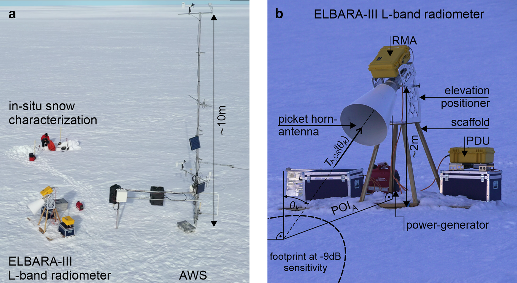
Fig. 1. Panel a: Experimental setup at Swiss Camp during May 2019 expedition. Panel b: Close-up picture of the ELBARA-III radiometer system.
Single angle $T_{{\rm A}\comma {\rm CR}}^p \lpar {\theta_{\rm A}} \rpar$ was continuously measured at the antenna nadir angle θ A = 60° and at polarizations p = {H, V}. In addition, three sets of multi-angle $T_{{\rm A}\comma {\rm CR}}^p \lpar {\theta_{\rm A}} \rpar$
 measurements at θ A = {30°, 40°, …, 90°} were conducted at anticipated SMOS local overpass times to compare against the corresponding spaceborne measurements $T_{{\rm SMOS}}^p \lpar {\theta_{\rm A}} \rpar$
 . Several sky measurements at θ A = 130° were also performed between 6 and 9 May 2019 for calibration purposes. Table 1 summarizes the ELBARA-III measurements collected in our study period at Swiss Camp.
Table 1. Summary of CR L-band radiometry at Swiss Camp between 6 and 10 May 2019
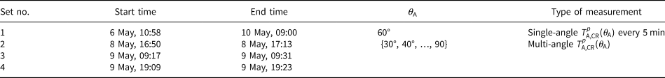
All times are given in local Greenland summer time (GMT-2).
3.3 In situ snow characterization
In situ snow profile measurements were conducted on 6 May at ~17:00 and on 9 May at ~11:00 and 19:00 to quantify snow properties during CR remote sensing at Swiss Camp. The latter two profiles capture the snowpack's temporal evolution mainly due to diurnal air temperature variations.
Profiles ρ S(z) and T S(z) of snow mass-density and snow temperature were taken close to the radiometer location (Fig. 1a) to best represent snow conditions within radiometer footprints. We used a 10-cm density cutter to measure ρ S, and T S was measured every 10 cm using an Extech Instruments Penetration Stem Dial Thermometer (Model 392050) with measurement accuracy and resolution of ±1° C and 0.1° C, respectively.
Examples of in situ ρ S(z) and T S(z) are shown in Figure 2. The top of the snowpack is at z = 0 m and its depth was ~80 cm during the study period. The temperature profile T S(z) depicted in Figure 2b is almost isothermal at T S ≈ 0° C (within the uncertainty of the applied thermometer), suggesting small amounts of snow liquid-water across the snowpack at the time of measurement.
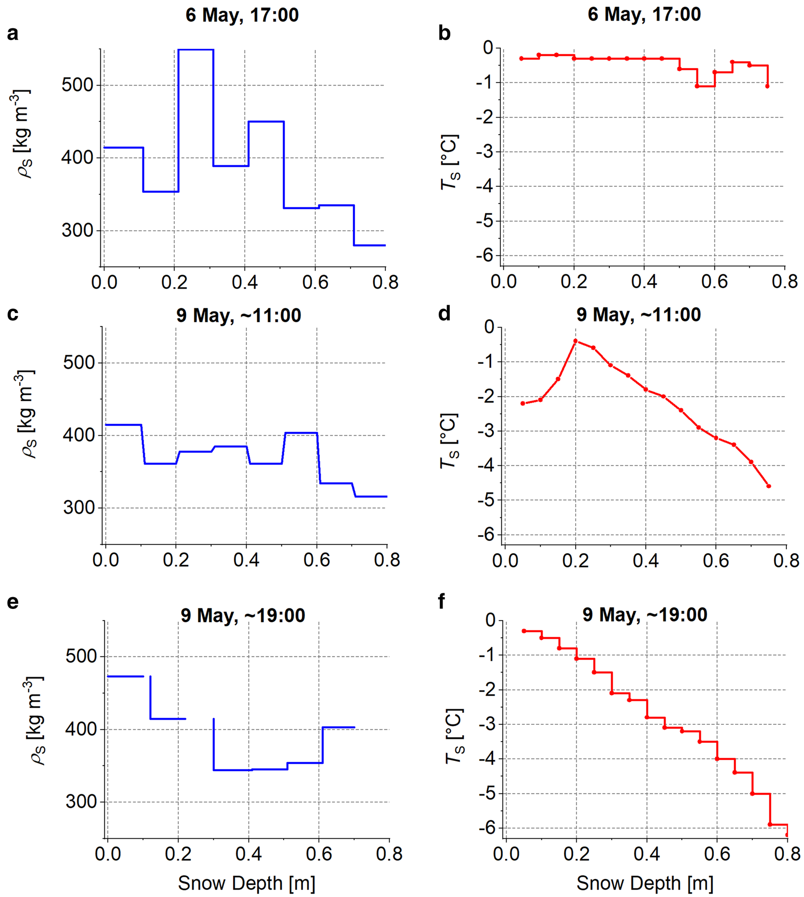
Fig. 2. Profiles of in situ snow mass-density ρ S(z) (panels a, c and e) and snow temperatures T S(z) (panels b, d and f) measured at Swiss Camp. Measurement times are given in local Greenland summer time (GMT-2).
Comparing this T S(z) against the two T S(z)-profiles measured on 9 May (Fig. 2d and f) highlights the change of the snowpack thermal state over 3 days of gradually decreasing air temperatures. The difference between T S(z) measured at 11:00 (Fig. 2d) and 19:00 (Fig. 2f) on 9 May reveals significant thermal changes of the snowpack. It implies appearance and disposition of liquid-water within the snowpack with a distinct variability, even within the short time span of 8 h. This observation is of practical relevance for remote sensing of snow melt, because it means that the time of acquisition can have a significant impact on snow wetness retrievals. As will be demonstrated in Section 5, this qualitative analysis of the temporal T S(z)-evolution is consistent with snow liquid water content retrieved from CR L-band radiometry at high temporal resolution.
4. Methodology
4.1 Computation of calibrated L-band antenna temperature
The final output derived from our L-band radiometer measurements are CR Antenna temperatures $T_{\rm A}^{p\comma ch} = T_{{\rm A}\comma {\rm CR}}^{p\comma ch}$ at polarization p = {H, V} and the two 11-MHz channels ch = {1, 2} within the protected part (1400–1427 MHz) of the L-band (1–2 GHz). Calibration of $T_{\rm A}^{p\comma ch}$
 relies on the sequential measurement of raw data (voltages) on at least two internal reference sources of known noise temperature. In the ELBARA-III (and ELBARA-II (Schwank and others, Reference Schwank2010)), three internal noise sources are implemented: (i) hot source (HS) of noise temperature $T_{{\rm HS}}^{ch}$
 realized with a noise diode; (ii) active cold source (ACS) of noise temperature $T_{{\rm ACS}}^{ch}$
 realized with a low noise amplifier (LNA) and (iii) matched resistive 50 Ω source (RS) of noise temperature $T_{{\rm RS}}^{ch}$
 . These internal references are installed on the calibration assembly (CA) inside the RMA (Fig. 1b). The CA is made of a copper block (1.7 kg) with high heat capacity and high thermal conductivity to minimize temperature variations in time and space. Under regular operation the CA is temperature stabilized, implying that reference noise temperatures $T_{{\rm HS}}^{ch}$
 , $T_{{\rm ACS}}^{ch}$
 , and $T_{{\rm RS}}^{ch}$
 are considered as constant between their calibration via sky measurements and their use as internal calibration sources during measurements toward footprints of interest (Fig. 1b). In case of stable physical temperature T CA of the CA, $T_{{\rm ACS}}^{ch}$
 is calibrated using simulated noise temperature of downwelling sky radiance T sky and the respective radiometer raw data $U_{{\rm sky}}^{p\comma ch}$
 (voltage) measured when the antenna is pointed toward the sky. The second reference noise source used to calibrate $T_{{\rm ACS}}^{ch}$
 is the RS with noise temperature $T_{{\rm RS}}^{ch} = T_{{\rm CA}}$
 and associated raw data $U_{{\rm RS}}^{ch}$
 . Finally, calibrated antenna temperature $T_{\rm A}^{p\comma ch}$
 is derived from raw data $U_{{\rm RMA}}^{p\comma ch}$
 measured for the antenna switched to the RMA input-ports p = {H, V}. Thereto, $T_{{\rm RS}}^{ch}$
 and $T_{{\rm ACS}}^{ch}$
 with associated $U_{{\rm RS}}^{ch}$
 and $U_{{\rm ACS}}^{ch}$
 known from previous sky calibration are used. Section 4 in Naderpour and others (Reference Naderpour, Schwank and Mätzler2017) provides a detailed description of the calibration procedure designed for the use with functional temperature stabilization of the RMA, meaning that T CA is considered as invariant between sky calibration of internal references and footprint measurements.
However, on 7 May 2019 the temperature stabilization of ELBARA-III RMA broke, meaning that T CA started to follow the air temperature T air. Consequently, gain and inherent noise of RMA components change between sky calibration of internal references and footprint measurements. In response, we developed the following calibration approach allowing to achieve calibrated Antenna temperatures $T_{\rm A}^{p\comma ch}$ even in the absence of instrument temperature control. The concept is to use multiple sky measurements performed over a range of T air resulting in varying T CA. This allows to characterize responses of noise temperatures $T_{{\rm ACS}}^{p\comma \;ch} \lpar {T_{{\rm CA}}} \rpar$
 and $T_{{\rm HS}}^{p\comma \;ch} \lpar {T_{{\rm CA}}} \rpar$
 with respect to their physical temperature T CA, and therefore to achieve calibrated $T_{\rm A}^{p\comma ch}$
 performed at T CA measured simultaneously.
At L-band, T sky is typically low (~5 K), stable in time, polarization independent and can be accurately simulated using e.g. the model described in Pellarin and others (Reference Pellarin2003). Therefore, the sky is known as a well-suited calibration target. However, noise temperature $T_{{\rm RMA}\comma {\rm sky}}^p$ at the RMA input-ports p = {H, V} during a sky measurement is larger than T sky entering the antenna aperture:

Here, $\Delta T_{{\rm TL}}^p$ expresses the noise added via transmission losses (TL) between the antenna and the RMA input ports:
Respective transmissivity $t_{{\rm TL}}^p$ is mainly due to losses $L_{{\rm TL}}^p = 0.18\;\;{\rm dB}$
 of the cables connecting the antenna ports p = {H, V} to the corresponding RMA input ports:
As mentioned, noise temperatures $T_{source}^{p\comma ch} \lpar {T_{{\rm CA}}} \rpar$ of the source = {ACS, HS} are calibrated for the range of T CA associated with the range of T air present during the series of sky measurements. This is achieved by using $T_{{\rm RMA}\comma {\rm sky}}^p$
 of sky observations in Eqns (1)–(3) and measured physical temperature T CA of the RS with noise temperature T RS = T CA together with measured raw data $U_{{\rm sky}}^{p\comma ch}$
 , $U_{{\rm RS}}^{ch}$
 and $U_{{\rm HS}}^{ch}$
 :
:

The sky measurement raw data $U_{{\rm sky}}^{p\comma ch}$ , which were least prone to radio frequency interference (according to the RFI quantification method described in Section 4.2 in Naderpour and others (Reference Naderpour, Schwank and Mätzler2017)), are used to derive T source(T CA) independent of p = {H, V} and ch = {1, 2}:


T ACS and T HS are in units of Kelvin and T CA is in units of °C. Antenna temperatures $T_{\rm A}^{p\comma ch}$ are calculated from associated raw data $U_{{\rm RMA}}^{p\comma ch}$
 :
:
4.1.1 Validation of calibration method
The $T_{\rm A}^{p\comma ch}$ calibration approach outlined in Section 4.1 for the ELBARA-III radiometer without temperature stabilization is used for the first time in this study. Therefore, we estimate the accuracy of measured CR antenna temperatures $T_{\rm A}^{p\comma ch} = T_{{\rm A}\comma {\rm CR}}^{p\comma ch}$
 calibrated by means of T ACS(T CA) and T HS(T CA) given by Eqn (5) and (6), respectively. Assessment of the calibration accuracy is done by computing the noise temperature $T_{{\rm RS}}^{ch}$
 of the RS from Eqn (7) when replacing $T_{\rm A}^{p\comma ch} \mapsto T_{{\rm RS}}^{ch}$
 and $U_{{\rm RMA}}^{p\comma ch} \mapsto U_{{\rm RS}}^{ch}$
 . Furthermore, we take advantage of the fact that, ideally noise temperature $T_{{\rm RS}}^{ch}$
 of the RS corresponds with its measured physical temperature T CA. Therefore, $\Delta T_{{\rm RS}}^{ch} \equiv \vert {T_{{\rm CA}}-T_{{\rm RS}}^{ch} } \vert$
 quantifies the uncertainty of our calibration approach developed for ELBARA-III with malfunctioning temperature control. Figure 3 shows the result of the assessment by means of a 4-day time series of T air, T CA and $T_{{\rm RS}}^{ch}$
 . Estimated calibration uncertainties $\Delta T_{{\rm RS}}^{ch}$
 for ch = {1, 2} are shown.
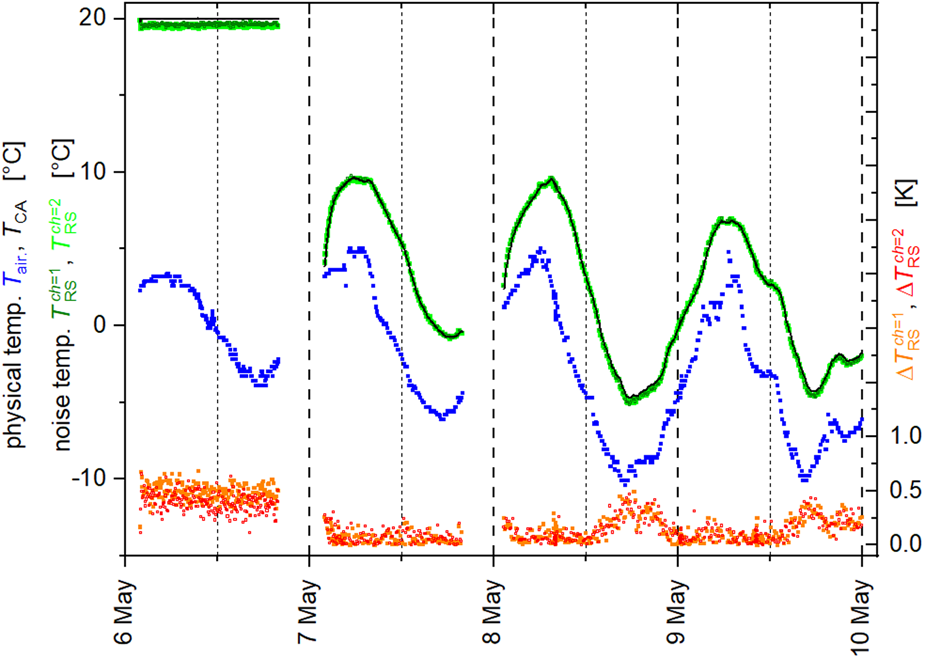
Fig. 3. Performance assessment of the calibration approach developed for malfunctioning temperature stabilization of ELBARA-III by means of time series of air temperature T air (blue), T CA (black) and $T_{{\rm RS}}^{ch}$ (light and dark green for ch = {1, 2}, respectively). Calibration uncertainties $\Delta T_{{\rm RS}}^{ch}$
 for ch = {1, 2} are shown in orange and red, respectively.
During the first ~18 h of the measurements, the temperature stabilization of ELBARA-III was fully functional, as evidenced by T CA ≅ 20°C while T air was significantly lower and varying with time. After the breakdown of ELBARA-III's temperature stabilization, T CA drops closer to T air and follows its temporal variability. Throughout the entire period, noise temperatures $T_{{\rm RS}}^{ch}$ are consistently $T_{{\rm RS}}^{ch} \cong T_{{\rm CA}}$
 . Respective calibration uncertainties $\Delta T_{{\rm RS}}^{ch} = \vert {T_{{\rm CA}}-T_{{\rm RS}}^{ch} } \vert$
 are consistently <0.7 K and are even smaller ($\Delta T_{{\rm RS}}^{ch} \lt 0.5{\rm \;K}$
 ) after the breakdown of the temperature stabilization as a result of lower T CA.
This analysis confirms the high accuracy of the calibration approach. Furthermore, it demonstrates that the overall performance of a radiometer which does not include any temperature stabilization can be as accurate as a corresponding temperature stabilized instrument. This technical insight is not the spotlight of this study; however, it is seen as an important message that could be relevant for the design of cost- and energy efficient radiometers especially useful to deploy in widespread areal networks in remote areas.
4.1.2 L-band measurement uncertainty
The uncertainty $\Delta T_{\rm A}^{p\comma ch} \lpar {\theta_{\rm A}} \rpar$ of calibrated CR antenna temperatures $T_{\rm A}^{p\comma ch} \lpar {\theta_{\rm A}} \rpar$
 is the root-mean-square error of three independent sources of uncertainty:

Uncertainty $\Delta T_{{\rm RFI}}^{p\comma ch} \lpar {\theta_{\rm A}} \rpar$ renders non-thermal RFI calculated using the methodology described in Section 4.2 of Naderpour and others (Reference Naderpour, Schwank and Mätzler2017). Concisely said, computation of $\Delta T_{{\rm RFI}}^{p\comma ch} \lpar {\theta_{\rm A}} \rpar$
 relies on fitting a Gaussian curve to the measurement samples $U_{{\rm RMA}}^{p\comma ch}$
 distribution which must be Gaussian for thermal emission. Therefore, the departure of $U_{{\rm RMA}}^{p\comma ch}$
 -distribution from Gaussian, is representative of non-thermal emission contribution. $\Delta T_{{\rm RS}}^{ch}$
 used in Eqn (8) reflects the calibration uncertainty explained in Section 4.1.1, and ELBARA-III's instrument radiometric uncertainty is estimated as ΔT ELBARA−III = 1 K (Schwank and others, Reference Schwank2010).
4.2 Emission model
A microwave EM inversion scheme is used to simultaneously estimate snow liquid water content (≡snow wetness) and snow mass-density (W S, ρ S). To implement this approach, L-band brightness temperatures $T_{\rm F}^p$ of facets (infinitesimal, horizontal and plane patches) within the antenna field-of-view (FoV) are simulated using the ‘L-Band Specific Microwave Emission Model of Layered Snow’ (LS-MEMLS) (Schwank and other, Reference Schwank2014; Naderpour and others, Reference Naderpour, Schwank and Mätzler2017). LS-MEMLS is a simplified version of MEMLS (Wiesmann and Mätzler, Reference Wiesmann and Mätzler1999; Mätzler and Wiesmann, Reference Mätzler and Wiesmann2012) in which volume scattering is neglected due to the significantly longer observation wavelength (λ = 21 cm) compared to snow microstructure. It is important to note that retrievals (W S, ρ S) are not derived directly from minimizing differences between brightness temperatures $T_{\rm F}^p$
 simulated with LS-MEMLS and measured antenna temperatures $T_{\rm A}^p$
 . Instead, it is the difference between simulated Antenna temperatures $T_{{\rm A}\comma {\rm sim}}^p$
 derived from the ensemble of brightness temperatures $T_{\rm F}^p \lpar {\theta_{\rm F}\comma \;\varphi_{\rm F}} \rpar$
 emitted by the facets within the antenna FoV seen at the facet elevation and azimuth angles θ F and φF, respectively. The model developed to transform the cumulative facet brightness temperatures $T_{\rm F}^p$
 into simulated antenna temperature $T_{{\rm A}\comma {\rm sim}}^p$
 is similar to the approach used in Volksch and others (Reference Volksch, Schwank, Stähli and Mätzler2015). Details of the respective modeling approach used in this study are outlined in Appendix A, whereas facet brightness temperatures $T_{\rm F}^p \lpar {\theta_{\rm F}} \rpar$
 at respective facet elevation angles θ F are simulated with the subsequently described version of LS-MEMLS.
In the general version of LS-MEMLS, the snowpack is modeled as j = 1,…,N horizontal and uniform snow layers stacked atop each other. Each layer is characterized by its thickness d j, physical temperature T j, dry mass density ρ j and volumetric liquid water content W j. The inputs to LS-MEMLS include observation nadir angle θ F, polarization p = {H, V}, and frequency f. Downwelling sky radiance T sky is simulated at f = 1.4 GHz using the model described in Pellarin and others (Reference Pellarin2003). Brightness temperatures $T_{\rm F}^p$ are simulated from the two-stream (2S) EM employed in MEMLS (Wiesmann and Mätzler, Reference Wiesmann and Mätzler1999; Mätzler and Wiesmann, Reference Mätzler and Wiesmann2012) and expressed as $T_{\rm F}^p = \sum\nolimits_{j = 0}^{N + 1} {a_j^p T_j}$
 where $a_j^p$
 are the Kirchhoff coefficients fulfilling $\sum\nolimits_{j = 0}^{N + 1} {a_j^p = 1}$
 . These coefficients weight the respective temperatures T 0 = T sub, T j (for j = 1, …, N), and T j+1 = T sky. The reader is referred to Schwank and others (Reference Schwank2014) and Naderpour and others (Reference Naderpour, Schwank and Mätzler2017) for more detailed description of LS-MEMLS.
In this study, an LS-MEMLS configuration identical to the one in Houtz and others (Reference Houtz, Naderpour, Schwank and Steffen2019) is considered. It comprises a two-layer snowpack above an infinite half-sphere of ice. The closed-form Kirchhoff coefficient formulas for this configuration are given in Section 2.2 of Houtz and others (Reference Houtz, Naderpour, Schwank and Steffen2019).
Figure 4 shows the employed configuration of LS-MEMLS whereby the concepts of SMOS satellite and CR radiometry are illustrated. This EM configuration adequately approximates the snowpack conditions in the ablation zone of the GrIS. The lowest layer in Figure 4 is the ice substrate (sub) with a specular interface with the overlaying snow. It is shown in Mätzler (Reference Mätzler2001) that near the Brewster angle, brightness temperatures at vertical polarization are least influenced by the snowpack. Strictly speaking the definition of a Brewster angle (θ Brewster = arctan(n 2/n 1) where n 2 and n 1 are the refractive indices of the regions containing the incident and the transmitted wave) is only applicable to a double-layer system (one interface). However, the cumulative Brewster effect of multiple dielectric interfaces leads to a Brewster-like angular behavior of emission at vertical polarization, meaning that emissivity at vertical polarization is maximal at a given observation angle. Considering the situation sketched with Figure 4, and assuming ice permittivity ɛsub = 3.18 (Koh, Reference Koh1997) and typical permittivity 1.3 ≤ ɛdry ≤ 1.8 of the overlaying dry snow-layer, the Brewster effect is most efficient within the angular range of 52.5° to 57.5°. Therefore, instead of introducing an additional ice temperature model, the effective ice temperature T sub is calculated using the time series mean of SMOS brightness temperatures at p = V and θ A = {52.5°, 57.5°} (see Section 2.2 of Houtz and others (Reference Houtz, Naderpour, Schwank and Steffen2019)).
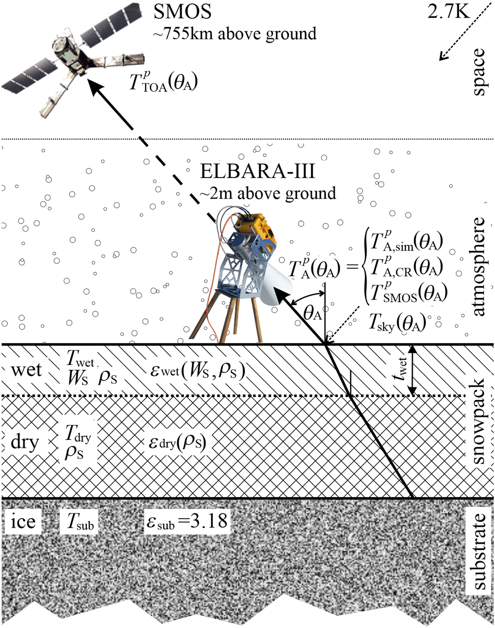
Fig. 4. The EM (LS-MEMLS) configuration used to simulate L-band brightness temperatures $T_{\rm F}^p \lpar {\theta_{\rm A}} \rpar$ of facets (infinitesimal, horizontal and plane patches) within the antenna FoV.
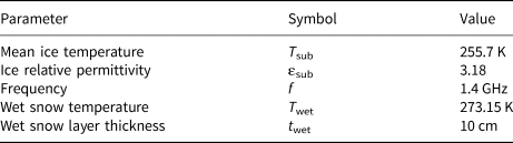
It is noteworthy that the emission depth in dry snow at L-band is larger than 100 m (Hofer and Mätzler, Reference Hofer and Mätzler1980; Mätzler and others, Reference Mätzler, Aebischer and Schanda1984) and thus much larger than snow depth in the ablation zone of the GrIS. Therefore, the dry snow layer in the EM configuration (Fig. 4) has a transmissivity of one; or in other words, it does not emit. However, the upper snow layer can have positive W S allowing for retrieval of liquid water content W S. Table 2 summarizes the key EM configuration parameters used in this paper.
Table 2. EM (LS-MEMLS) configuration parameters
4.3 Multi-angle retrieval approach
The approach for the simultaneous retrieval of (W S, ρ S) is based on optimally fitting simulated antenna temperatures $T_{{\rm A}\comma {\rm sim}}^p \lpar {\theta_{\rm A}} \rpar$ to multi-angle antenna temperatures $T_{\rm A}^p \lpar {\theta_{\rm A}} \rpar = T_{{\rm A}\comma {\rm CR}}^p \lpar {\theta_k} \rpar$
 or $T_{\rm A}^p \lpar {\theta_{\rm A}} \rpar = T_{{\rm SMOS}}^p \lpar {\theta_{\rm A}} \rpar$
 measured with ELBARA-III or SMOS, respectively. Again, it is noted that simulated antenna temperatures are achieved by first simulating brightness temperatures $T_{\rm F}^p$
 of facets within the radiometer footprint using LS-MEMLS (Section 4.2), which are then aggregated to $T_{{\rm A}\comma {\rm sim}}^p \lpar {\theta_{\rm A}} \rpar$
 using the approach outlined in Appendix A.
With two unknown parameters and multiple known pairs of $T_{\rm A}^p \lpar {\theta_k} \rpar$ measured at several observation nadir angles θ A and p = {H, V}, the retrievals (W S, ρ S) are the solution of an overdetermined system of equations. To reach the optimal fit, the Cost Function (CF) below is devised and minimized:
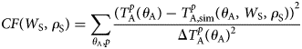
The equation above quantifies the sum of squared differences between measured nadir angle scan sets $T_{\rm A}^p \lpar {\theta_{\rm A}} \rpar$ and corresponding simulated $T_{{\rm A}\comma {\rm sim}}^p \lpar {\theta_k} \rpar$
 for given values of (W S, ρ S) at p = {H, V}. The $\Delta T_{\rm A}^p \lpar {\theta_{\rm A}} \rpar$
 in the denominator (computed with Eqn (8)) considers the effect of measurement uncertainties in the retrievals (W S, ρ S). A global numerical optimization process is run to minimize the CF by tuning (W S, ρ S). The corresponding parameters for which CF is minimized are taken as retrieval results.
4.4 Single-angle retrieval approach
Similar to the multi-angle retrieval approach, the single-angle retrieval approach relies on optimally fitting simulated antenna temperatures to measured data. When the objective is retrieval of two state parameters (W S and ρ S) from two measurements $T_{\rm A}^{\rm H} \lpar {\theta_{\rm A}} \rpar$ and $T_{\rm A}^{\rm V} \lpar {\theta_{\rm A}} \rpar$
 at a single nadir angle θ A, the mathematical problem to solve is no longer overdetermined unlike the case for multi-angle retrievals explained in Section 4.3. The single-angle retrieval approach is based on solving the equation system below:
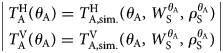
These two equations are solved numerically to find $\;\lpar {W_{\rm S}^{\theta_{\rm A}} \comma \;\rho_{\rm S}^{\theta_{\rm A}} } \rpar$ where the retrieved parameters can vary within $0\,{\rm m}^3{\rm m}^{{-}3} \le W_{\rm S}^{\theta _{\rm A}} \! \le&InLnBrk; \! 0.9\,\;{\rm m}^3\,{\rm m}^{{-}3}$
 and $150 \;{\rm kg\;}{\rm m}^{{-}3} \! \le \! \rho _{\rm S}^{\theta _{\rm A}} \le 600 \;{\rm kg\;}{\rm m}^{{-}3} \!$
 . It is noteworthy that single-angle retrievals $\lpar {W_{\rm S}^{\theta_{\rm A}} \comma \;\rho_{\rm S}^{\theta_{\rm A}} } \rpar$
 are expected to be more prone to errors in measured and simulated antenna temperatures. Also, it is apparent from Eqn (10) that, measurement uncertainties cannot be considered in single-angle retrievals $\lpar {W_{\rm S}^{\theta_{\rm A}} \comma \;\rho_{\rm S}^{\theta_{\rm A}} } \rpar$
 . Furthermore, all single-angle ELBARA-III measurements used in our study were performed at θ A = 60°. Therefore, henceforth we indicate the single-angle retrievals with $\;\lpar {W_{\rm S}^{60} \comma \;\rho_{\rm S}^{60} } \rpar$
 .
.
5. Results and discussion
Due to considerable diurnal fluctuations of air temperature ~0°C during May 2019 measurements at Swiss Camp, the snowpack underwent major changes including melt–refreeze cycles. Such changes were partially captured and demonstrated with in situ measurements shown in Section 3. Responses of single- and multi-angle satellite (SMOS) and CR (ELBARA-III) microwave measurements to temporal variations of snowpack conditions are presented in Sections 5.1.1 and 5.1.2, respectively. Finally, Section 5.2 presents snow wetness retrieved from CR single-angle antenna temperatures (Section 5.2.1) and from corresponding multi-angle measurements (Section 5.2.2).
5.1 Close-range and SMOS measurements
5.1.1 Single-angle antenna temperatures
Figure 5 shows the time series of CR single-angle antenna temperatures $T_{{\rm A}\comma {\rm CR}}^p \lpar {\theta_{\rm A} = 60^\circ } \rpar$ measured with ELBARA-III and corresponding bottom-of-atmosphere SMOS $T_{{\rm SMOS}}^p \lpar {\theta_{\rm A} = 60^\circ } \rpar$
 in panel a, as well as air temperature T air in panel b. A 30-min asymmetric sliding average is run over the respective L-band measurements. Close to our experimental setup at Swiss Camp, two sources of RFI were detected, both of which introduced occasional disturbances in the measurements: (i) a portable gasoline-powered generator which was operated ~10 m from ELBARA-III, and (ii) a TX321 satellite transmitter at the AWS, which uplinks the meteorological data every hour. In total, 75 highly RFI-corrupted $T_{{\rm A}\comma {\rm CR}}^p \lpar {\theta_{\rm A} = 60^\circ } \rpar$
 were eliminated from the time series by means of median absolute deviation filtering.

Fig. 5. Panel a shows time series of CR ELBARA-III antenna temperatures $T_{{\rm A}\comma {\rm CR}}^p \lpar {\theta_{\rm A} = 60^\circ } \rpar$ at horizontal (p = H, small red symbols) and vertical (p = V, small blue symbols) polarization. SMOS $T_{{\rm SMOS}}^p \lpar {\theta_{\rm A} = 60^\circ } \rpar$
 are shown with large red symbols for p = H and with large blue symbols for p = V. T air measured with ELBARA-III's external PT-100 sensor is shown in panel b.
SMOS-measured $T_{{\rm SMOS}}^{\rm H} \lpar {\theta_{\rm A} = 60^\circ } \rpar$ and $T_{{\rm SMOS}}^{\rm V} \lpar {\theta_{\rm A} = 60^\circ } \rpar$
 are shown with bold red and blue symbols in Figure 5a. It is worth noting that SMOS L3 brightness temperatures does not include $T_{{\rm SMOS}}^p \lpar {\theta_{\rm A}} \rpar$
 at exactly θ A = 60°. Hence, a spline fit is used to interpolate $T_{{\rm SMOS}}^p \lpar {\theta_{\rm A} = 60^\circ } \rpar$
 from other SMOS observations available at the nadir angles mentioned in Section 3.
The time series of T air (Fig. 5b), measured with ELBARA-III's PT-100 sensor shows diurnal fluctuations around the freezing point at 0°C such that every day the air temperature is positive for several hours in the afternoon before gradually dropping to its minimum below freezing point in early morning.
Measured T air shows roughly an anticorrelation with $T_{{\rm A}\comma {\rm CR}}^{\rm H} \lpar {\theta_{\rm A} = 60^\circ } \rpar$ . Timing of local maxima in T air is close to the timing of local minima in $T_{{\rm A}\comma {\rm CR}}^{\rm H} \lpar {\theta_{\rm A} = 60^\circ } \rpar$
 with a typical lag of a few hours. Furthermore, T air shows a decreasing trend beneath the diurnal oscillations, while $T_{{\rm A}\comma {\rm CR}}^p \lpar {\theta_{\rm A} = 60^\circ } \rpar$
 at both polarizations show an increasing trend.
Dry snow (with emission depth of >100 m (Hofer and Mätzler, Reference Hofer and Mätzler1980; Mätzler and others, Reference Mätzler, Aebischer and Schanda1984)) does not emit at L-band but impacts brightness temperature via refraction and impedance matching (Schwank and others, Reference Schwank2014, Reference Schwank2015). However, a moist snow-layer with increasing W S, starts emitting while reflectivities at its boundaries increase at the same time. Previous sensitivity analyses (Naderpour and others, Reference Naderpour, Schwank and Mätzler2017), based on LS-MEMLS, revealed that brightness temperature first increases with growing W S for low liquid water contents, while it decreases with W S for higher liquid water contents. The initial increase in brightness temperature is due to enhanced snow emission, which is eventually overtaken by increased reflectivities at yet larger W S resulting in decreasing brightness temperature. Furthermore, it is known that vertically polarized brightness temperature at observations angles (θ A ≈ 60°) most affected by the Brewster effect (Section 4.2) is distinctly less influenced by the snowpack than corresponding brightness temperature at horizontal polarization (Schwank and others, Reference Schwank2015). In agreement with this, diurnal fluctuations of $T_{{\rm A}\comma {\rm CR}}^{\rm H} \lpar {\theta_{\rm A} = 60^\circ } \rpar$ are clearly exceeding diurnal fluctuations $T_{{\rm A}\comma {\rm CR}}^{\rm V} \lpar {\theta_{\rm A} = 60^\circ } \rpar$
 as is apparent in Figure 5a.
The pronounced diurnal minima of $T_{{\rm A}\comma {\rm CR}}^{\rm H} \lpar {\theta_{\rm A} = 60^\circ } \rpar$ indicate that snow wetness reaches significantly high values during afternoons with T air > 0°C. These diurnal minima of ELBARA-III antenna temperatures take place between 3 h 10 min and 1 h 10 min later than T air reaches its maximum during afternoons. These time lags between the minima of $T_{{\rm A}\comma {\rm CR}}^{\rm H} \lpar {\theta_{\rm A} = 60^\circ } \rpar$
 and the maxima of T air are due to thermal inertia associated with ice latent-heat and the snowpack's thermal inertia (Pomeroy and Brun, Reference Pomeroy and Brun2001). As explained previously, $T_{{\rm A}\comma {\rm CR}}^p \lpar {\theta_{\rm A} = 60^\circ } \rpar$
 , especially at p = H, is expected to increase for small W S where increasing emission of moist snow dominates. We hypothesize that the timestamps T1, T2 and T3 (indicated in Fig. 5a) are demonstrations of this effect, which causes $T_{{\rm A}\comma {\rm CR}}^{\rm H} \lpar {\theta_{\rm A} = 60^\circ } \rpar$
 to increase for a short time due to lightly moist snow, before $T_{{\rm A}\comma {\rm CR}}^{\rm H} \lpar {\theta_{\rm A} = 60^\circ } \rpar$
 decreases due to yet higher W S. It is likely that the short-term increases apparent in $T_{{\rm A}\comma {\rm CR}}^{\rm H} \lpar {\theta_{\rm A} = 60^\circ } \rpar$
 at the afternoon times T1 and T3 are due to pre-melting, while the short-term increase in $T_{{\rm A}\comma {\rm CR}}^{\rm H} \lpar {\theta_{\rm A} = 60^\circ } \rpar$
 during the night-time T2 is interpreted as a result of refreezing. It is worth noting that the aforementioned diurnal and even inter-diurnal changes in snow wetness are apparent in measured L-band antenna temperatures.
A closer look at T air in Figure 5b reveals a general cooling trend in air temperature. While T air does rise above 0°C every day, both the duration of T air > 0° C and its daily extremes decrease over the study period. Consequently, the minimum of $T_{{\rm A}\comma {\rm CR}}^{\rm H} \lpar {\theta_{\rm A} = 60^\circ } \rpar$ gradually increases from ~140 to ~210 K. If $\Delta T_{{\rm A}\comma {\rm CR}}^{\rm H} \lpar {\theta_{\rm A} = 60^\circ } \rpar$
 is defined as the dynamics of $T_{{\rm A}\comma {\rm CR}}^{\rm H} \lpar {\theta_{\rm A} = 60^\circ } \rpar$
 in a full diurnal cycle, it decreases from ~48.5 K on 7 May to ~11.2 K on 9 May.
Despite their statistically limited number, SMOS brightness temperatures $T_{{\rm SMOS}}^{\rm H} \lpar {\theta_{\rm A} = 60^\circ } \rpar$ in Figure 5a show relative consistency with CR antenna temperatures $T_{{\rm A}\comma {\rm CR}}^{\rm H} \lpar {\theta_k = 60^\circ } \rpar$
 temporal variations. For example, $T_{{\rm SMOS}}^{\rm H} \lpar {\theta_{\rm A} = 60^\circ } \rpar$
 for the afternoon overpasses are consistently lower than $T_{{\rm SMOS}}^{\rm H} \lpar {\theta_{\rm A} = 60^\circ } \rpar$
 for early morning visits, indicating the response to changed snowpack wetness. As another example, $T_{{\rm SMOS}}^{\rm H} \lpar {\theta_{\rm A} = 60^\circ } \rpar$
 measurements in the evening of 7 May and morning of 8 May, follow an increasing trend similar to the CR $T_{{\rm A}\comma {\rm CR}}^{\rm H} \lpar {\theta_{\rm A} = 60^\circ } \rpar$
 in response to snowpack refreezing.
The discrepancies between SMOS and ELBARA-III measurements may root partially in the much larger footprint size of SMOS (diameter of ~25 km) compared to the CR footprints (several square meters) which introduces significantly larger spatial heterogeneities of SMOS footprints compared to CR footprints. Spline interpolation was used to interpolate SMOS brightness temperatures to the coordinates of Swiss Camp from the surrounding pixel center coordinates. Smooth spline interpolation may not be optimal during diurnally oscillating snow-wetness periods because there may be pixels containing wet- and dry snow or even standing water, leading to a blurring in the single-point interpolation.
Both $T_{{\rm A}\comma {\rm CR}}^{\rm V} \lpar {\theta_{\rm A} = 60^\circ } \rpar$ and $T_{{\rm SMOS}}^{\rm V} \lpar {\theta_{\rm A} = 60^\circ } \rpar$
 at vertical polarization show much less sensitivity to snowpack moisture variations compared to horizontal polarization. This lack of sensitivity at θ A = 60° agrees with the expectation based on the Brewster effect discussed above.
5.1.2 Satellite and close-range multi-angle measurements
Figure 6 shows multi-angle SMOS $T_{{\rm SMOS}}^p \lpar {\theta_{\rm A}} \rpar$ together with ELBARA-III $T_{{\rm A}\comma {\rm CR}}^p \lpar {\theta_{\rm A}} \rpar$
 at the SMOS overpass on 9 May 2019 at ~19:30 local time. The error bars associated with $T_{{\rm A}\comma {\rm CR}}^p \lpar {\theta_{\rm A}} \rpar$
 are calculated using Eqn (8) and the error bars associated with $T_{{\rm SMOS}}^p \lpar {\theta_{\rm A}} \rpar$
 are equivalent to $\sigma T_{{\rm SMOS}}^p \lpar {\theta_{\rm A}} \rpar$
 whose method of computation is described in Section 3.
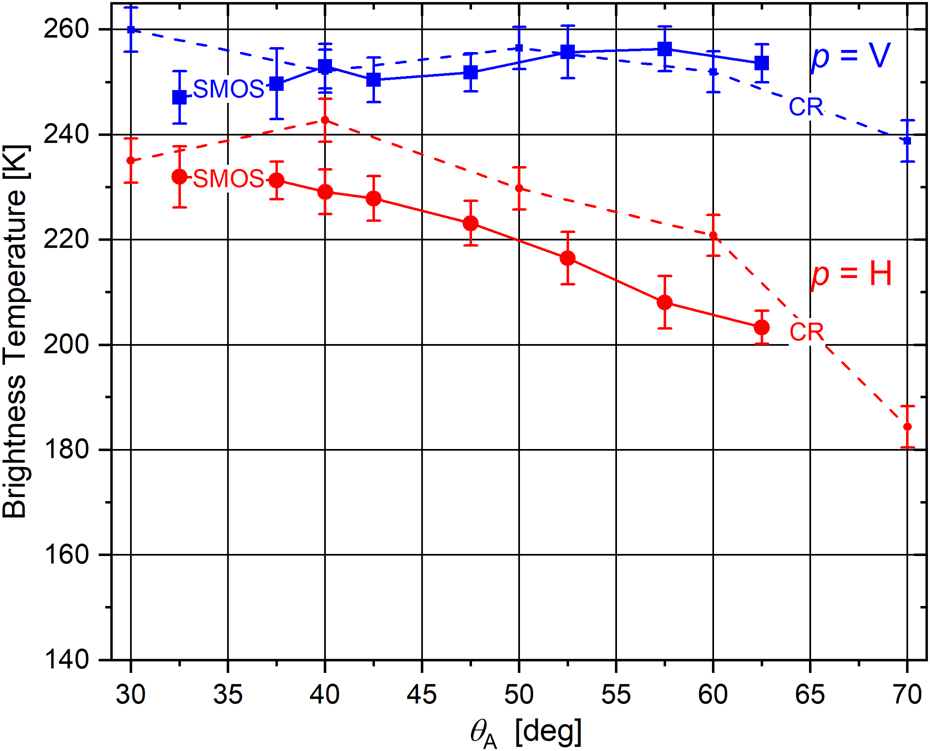
Fig. 6. Multi-angle SMOS and CR $T_{{\rm SMOS}}^p \lpar {\theta_{\rm A}} \rpar$ and $T_{{\rm A}\comma {\rm CR}}^p \lpar {\theta_{\rm A}} \rpar$
 , respectively, at Swiss Camp on 9 May 2019 at ~19:30 local Greenland summer time (GMT-2). Error bars at each point indicate the corresponding measurement uncertainties.
The consistency of single-angle CR $T_{{\rm A}\comma {\rm CR}}^p \lpar {\theta_{\rm A} = 60^\circ } \rpar$ measurements with the SMOS $T_{{\rm SMOS}}^p \lpar {\theta_{\rm A} = 60^\circ } \rpar$
 is demonstrated in Figure 5. Additionally, multi-angle measurements such as shown in Figure 6, were conducted to investigate the agreement between snapshots of SMOS $T_{{\rm SMOS}}^p \lpar {\theta_{\rm A}} \rpar$
 and CR $T_{{\rm A}\comma {\rm CR}}^p \lpar {\theta_{\rm A}} \rpar$
 radiometry at multiple observation nadir angles θ A. The microwave temperatures provided in Figure 6 agree within a 95% confidence interval, approximately three times the displayed single standard error bar magnitudes.
LS-MEMLS simulations of a snowpack with given (W S, ρ S) show that brightness temperatures at vertical polarization must be higher than at horizontal polarization for a given nadir angle (Section 4 in Houtz and others (Reference Houtz, Naderpour, Schwank and Steffen2019)). Therefore, the arrangement between $T_{{\rm SMOS}}^p \lpar {\theta_{\rm A}} \rpar$ and $T_{{\rm A}\comma {\rm CR}}^p \lpar {\theta_{\rm A}} \rpar$
 in Figure 6 are consistent with theoretical expectation. Furthermore, the angular pattern of $T_{{\rm SMOS}}^p \lpar {\theta_{\rm A}} \rpar$
 and $T_{{\rm A}\comma {\rm CR}}^p \lpar {\theta_{\rm A}} \rpar$
 are in good agreement with each other especially for $\theta _{\rm A}{\rm \lesssim }65^\circ$
 where $T_{{\rm SMOS}}^p \lpar {\theta_{\rm A}} \rpar$
 are available and emission contribution to ELBARA-III $T_{{\rm A}\comma {\rm CR}}^p \lpar {\theta_{\rm A}} \rpar$
 from the atmosphere is insignificant. The error bars in Figure 6 highlight this agreement where most of $T_{{\rm SMOS}}^p \lpar {\theta_{\rm A}} \rpar$
 fall within the range of $T_{{\rm A}\comma {\rm CR}}^p \lpar {\theta_{\rm A}} \rpar$
 especially for p = V.
The spatial heterogeneities in large SMOS pixels (diameter of ~25 km) cause an unknown amount of bias in the absolute values of $T_{{\rm SMOS}}^p \lpar {\theta_{\rm A}} \rpar$ with respect to $T_{{\rm A}\comma {\rm CR}}^p \lpar {\theta_{\rm A}} \rpar$
 . Nevertheless, the consistency of the angular pattern of large-scale $T_{{\rm SMOS}}^p \lpar {\theta_{\rm A}} \rpar$
 with CR $T_{{\rm A}\comma {\rm CR}}^p \lpar {\theta_{\rm A}} \rpar$
 can be seen as an experimental sanity check of the spatial interpolation method adopted in Houtz and others (Reference Houtz, Naderpour, Schwank and Steffen2019) for calculating $T_{{\rm SMOS}}^p$
 .
.
5.2 Retrievals of volumetric snow liquid water content
Single- and multi-angle L-band measurements, presented in Section 5.1, are used to retrieve volumetric snow liquid water content (≡snow wetness) W S based on the approaches discussed in Sections 4.3 and 4.4. From the simultaneously retrieved snow wetness and snow mass-density (W S, ρ S), we only demonstrate and discuss W S-retrievals due to several reasons: first, W S-retrievals are the focus of this paper and undergo noticeable and rapid diurnal changes as opposed to ρ S which does not change significantly over a few days. Furthermore, as shown in (Houtz and others, Reference Houtz, Naderpour, Schwank and Steffen2019), while ρ S-retrievals are sensible in their long-term monthly and seasonal averages, in short-term ρ S is a semi-free parameter in the retrieval procedure assisting with more accurate retrieval of W S.
5.2.1 Retrievals from single-angle close-range measurements
Sensitivities of ELBARA-III $T_{{\rm A}\comma {\rm CR}}^p \lpar {\theta_{\rm A} = 60^\circ } \rpar$ and SMOS $T_{{\rm SMOS}}^p \lpar {\theta_{\rm A} = 60^\circ } \rpar$
 to snow wetness and its temporal variations were experimentally demonstrated and discussed in Section 5.1.1. The approach explained in Section 4.4 is used to retrieve $W_{{\rm S}\comma {\rm CR}}^{60}$
 from CR single-angle antenna temperatures $T_{{\rm A}\comma {\rm CR}}^p \lpar {\theta_{\rm A} = 60^\circ } \rpar$
 . Figure 7a shows the time series of the corresponding retrievals $W_{{\rm S}\comma {\rm CR}}^{60}$
 accompanied by air temperature T air measured by the PT-100 sensor attached to ELBARA-III as shown in Figure 7b.
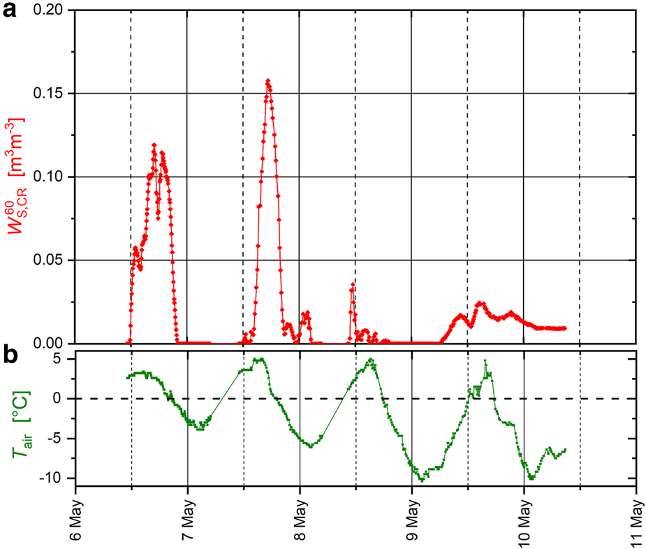
Fig. 7. (a) Time series of snow wetness retrievals $W_{{\rm S}\comma {\rm CR}}^{60}$ based on single-angle $T_{{\rm A}\comma {\rm CR}}^p \lpar {\theta_{\rm A} = 60^\circ } \rpar$
 measurement conducted with ELBARA-III at Swiss Camp. (b) T air measured with the external PT-100 sensor. Two gaps in the time series (05:00–11:00 on 7 May and 04:50–10:20 on 8 May) are due to system shutdown resulting from power cuts.
Figure 7 shows that $W_{{\rm S}\comma {\rm CR}}^{60}$ captures the diurnal melt/refreeze cycles of the snowpack. When T air exceeds 0°C, $W_{{\rm S}\comma {\rm CR}}^{60}$
 follows suit with some delay. $W_{{\rm S}\comma {\rm CR}}^{60}$
 reaches its maximum lagging behind T air by 1–3 h on each day. The gradual cooling of T air during the study period also manifests its effects in lower $W_{{\rm S}\comma {\rm CR}}^{60}$
 values from 7 to 10 May 2019. Both of the aforementioned temporal behaviors of retrieved $W_{{\rm S}\comma {\rm CR}}^{60}$
 are fully consistent with the finding made from the discussion of $T_{{\rm A}\comma {\rm CR}}^p \lpar {\theta_{\rm A} = 60^\circ } \rpar$
 and $T_{{\rm SMOS}}^p \lpar {\theta_{\rm A} = 60^\circ } \rpar$
 presented in Section 5.1.1.
To address different possible scenarios of liquid-water distribution along the snow-profile, $W_{{\rm S}\comma {\rm CR}}^{60}$ retrieval sensitivity analyses have been performed using EM (LS-MEMLS) configurations with corresponding layering of moist- and dry snow. These EM configurations included: (a) snowpack with a potentially wet snow-layer of thickness in the range 10 cm ≤ t wet ≤ 20 cm atop dry snow (Fig. 4), and (b) single-layer snowpack with uniform snow liquid water content. The results conclude that the temporal variations of retrievals $W_{{\rm S}\comma {\rm CR}}^{60}$
 indicating melt/refreeze cycles are largely independent of the employed EM configuration. However, the magnitudes of $W_{{\rm S}\comma {\rm CR}}^{60}$
 exhibit some dependency on the EM configuration. Nevertheless, the analysis of $W_{{\rm S}\comma {\rm CR}}^{60}$
 sensitivity with respect to the mentioned snowpack configurations still suggest that our physics-based retrieval approach is fairly robust, and therefore applicable during different seasons over the ablation zone of the GrIS.
5.2.2 Retrievals from multi-angle measurements
The three sets of ELBARA-III CR multi-angle antenna temperatures $T_{{\rm A}\comma {\rm CR}}^p \lpar {\theta_{\rm A}} \rpar$ , listed in Table 1, were used to retrieve snow liquid water content W S,CR based on the method described in Section 4.3. These multi-angle retrievals together with respective single-angle retrievals $W_{{\rm S}\comma {\rm CR}}^{60}$
 and measured T air are shown in Figure 8.
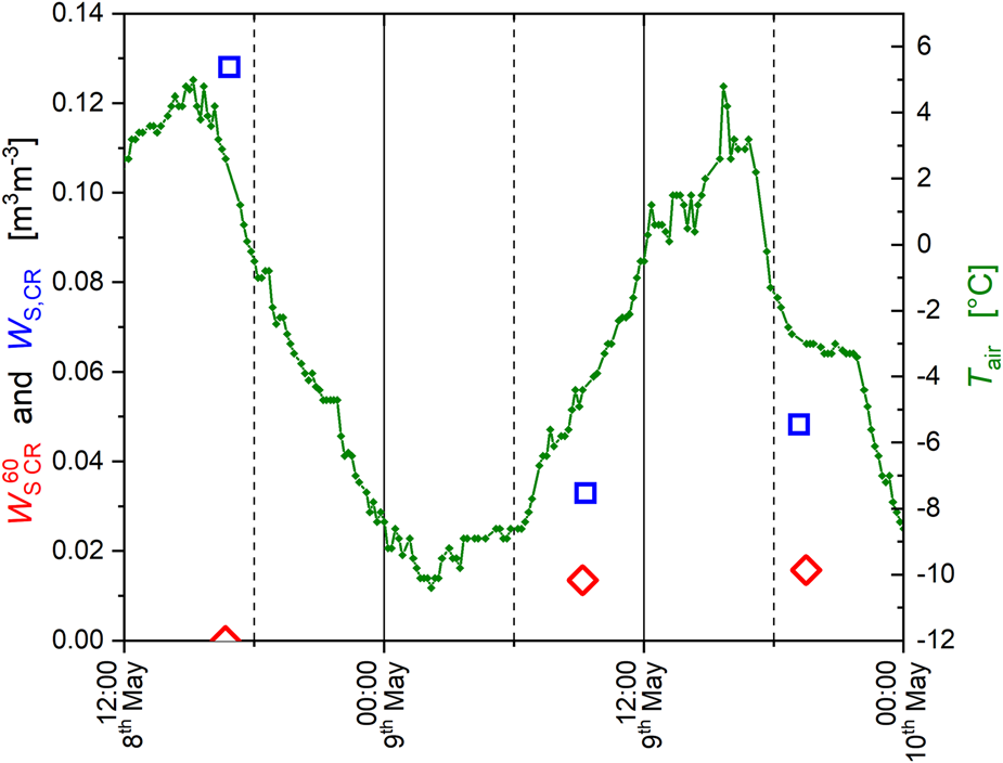
Fig. 8. Left axis: Snow wetness W S,CR (blue squares) and $W_{{\rm S}\comma {\rm CR}}^{60}$ (red diamonds) retrieved from multi- and single-angle CR antenna temperatures. Right axis: Air temperature T air (green) measured with ELBARA-III's external PT-100 sensor.
Multi-angle retrievals W S,CR (blue squares) during the afternoon of 8 and 9 May detect liquid water in the snow. This corresponds well with the expected increased snow wetness after several hours of T air > 0°C. In the morning of 9 May (at ~12:20) retrieved snow wetness is distinctly lower, indicating a partial refreezing of the snowpack which took place over night with T air < 0° C. On 9 May, the single-angle retrievals $W_{{\rm S}\comma {\rm CR}}^{60}$ (red diamonds) in Figure 8 corroborate the multi-angle W S,CR retrievals in terms snow melt detection. However, there is a clear discrepancy between single- and multi-angle retrievals on 8 May. The reason for this discrepancy may be spatial heterogeneities observed with multi-angle measurements and the effect of considering measurement uncertainties in the multi-angle retrieval approach (Eqn (9)) which is missing in single-angle retrievals. The statistically limited set of multi-angle measurements prohibit detailed investigation of the agreement between retrievals W S,CR and $W_{{\rm S}\comma {\rm CR}}^{60}$
 . Nevertheless, it is prudent to conduct such a study with SMOS observations.
There is only one set of multi-angle CR $T_{{\rm A}\comma {\rm CR}}^p \lpar {\theta_{\rm A}} \rpar$ available from our ELBARA-III measurements which is close in time to a local SMOS overpass. However, our investigations show that snow liquid water content retrieved from multi-angle $T_{{\rm SMOS}}^p \lpar {\theta_{\rm A}} \rpar$
 agree well with quasi-simultaneous single-angle retrievals $W_{{\rm S}\comma {\rm CR}}^{60}$
 based on $T_{{\rm A}\comma {\rm CR}}^p \lpar {\theta_{\rm A} = 60^\circ } \rpar$
 in terms of snow wetness detection and its temporal variations.
6. Conclusion
An inversion-based retrieval approach (using LS-MEMLS as forward model) for the estimation of snow wetness over the GrIS using SMOS observations was introduced in Houtz and others (Reference Houtz, Naderpour, Schwank and Steffen2019). However, this investigation lacked in situ validation and could only compare results to other satellite-based empirical wetness retrieval algorithms. The initial goal of this study was in-depth investigation and validation of the retrieval approach in Houtz and others (Reference Houtz, Naderpour, Schwank and Steffen2019) using CR radiometry with high temporal and spatial resolution and accompanied this with in situ characterization of the snowpack. However, the findings of this study reached beyond the initially defined goals. First, we validated the findings of Houtz and others (Reference Houtz, Naderpour, Schwank and Steffen2019) by demonstrating that the physics-based retrieval approach provides meaningful results also using CR L-band antenna temperatures; second, we showed that snow wetness over the GrIS can be estimated from passive L-band measurements at a single observation angle. Third, with the failure of ELBARA-III's temperature stabilization system and consequently the conventional calibration method, an alternative calibration approach was devised to achieve calibrated CR antenna temperatures $T_{{\rm A}\comma {\rm CR}}^p$ . Fourth, the relatively wide FoV of ELBARA-III's Pickett horn antenna required the development of an approach to transform simulated brightness temperatures emitted by facets within the footprint to antenna temperatures ultimately used for retrievals. Even though the third and fourth developments are not the focus of our scientific investigation, these technical achievement are relevant for: (i) the design of cost- and energy efficient microwave radiometers, especially for their deployment in widespread areal networks in remote areas, and (ii) the scientific interpretation of CR passive microwave measurements performed with antennas featuring wide FoV's.
Agreement between SMOS brightness temperatures $T_{{\rm SMOS}}^p$ and CR antenna temperatures $T_{{\rm A}\comma {\rm CR}}^p$
 for single- and multi-angle measurements was shown to be within the 95% confidence intervals with respect to their measurement uncertainty. Single-angle measurements $T_{{\rm SMOS}}^{\rm V} \lpar {\theta_{\rm A} = 60^\circ } \rpar$
 and $T_{{\rm A}\comma {\rm CR}}^{\rm V} \lpar {\theta_{\rm A} = 60^\circ } \rpar$
 exhibit much less sensitivity to the snowpack's temporal variations due to the Brewster effect. This further validates the approach adopted in Houtz and others (Reference Houtz, Naderpour, Schwank and Steffen2019) to use $T_{{\rm A}\comma {\rm SMOS}}^{\rm V}$
 measured at nadir angles where Brewster effects are most efficient to estimate substrate (ice) temperature T sub.
Responses of ELBARA-III $T_{{\rm A}\comma {\rm CR}}^{\rm H} \lpar {\theta_{\rm A} = 60^\circ } \rpar$ to snow liquid water content W S were consistent with simulations achieved with LS-MEMLS representing the snowpack with two layers. Furthermore, $T_{{\rm A}\comma {\rm CR}}^{\rm H} \lpar {\theta_{\rm A} = 60^\circ } \rpar$
 provided experimental proof to the sensitivity analysis of Naderpour and others (Reference Naderpour, Schwank and Mätzler2017), corroborating that little amounts of W S increases brightness temperature due to snow self-emission, while brightness temperature is decreased due to dominating reflectivity for higher snow wetness.
Comparison between quasi-simultaneous multi-angle $T_{{\rm SMOS}}^p \lpar {\theta_{\rm A}} \rpar$ and $T_{{\rm A}\comma {\rm CR}}^p \lpar {\theta_{\rm A}} \rpar$
 shows agreement between the respective angular patterns and agreement in their magnitudes. This agreement indicates the sanity of the spatial-interpolation and atmospheric correction methods adopted in Houtz and others (Reference Houtz, Naderpour, Schwank and Steffen2019) for the computation of $T_{{\rm SMOS}}^p \lpar {\theta_{\rm A}} \rpar$
 at a given point over the GrIS. The slight bias of $T_{{\rm SMOS}}^p \lpar {\theta_{\rm A}} \rpar$
 with respect to CR $T_{{\rm A}\comma {\rm CR}}^p \lpar {\theta_{\rm A}} \rpar$
 are hypothesized to be due to spatial heterogeneities in the large SMOS footprints.
Our investigations also demonstrate that snow wetness can not only be retrieved from multi-angle measurements, but also from a pair of single-angle $T_{{\rm A}\comma {\rm CR}}^p \lpar {\theta_{\rm A} = 60^\circ } \rpar$ at polarizations p = {H, V}. This means that even though, as opposed to the multi-angle retrieval approach, the equation system for the retrieval of $\;W_{\rm S}^{60}$
 is no longer over-determined, it can still yield reliable results. Multi-angle retrievals W S,CR and their comparison with single-angle retrievals $W_{{\rm S}\comma {\rm CR}}^{60}$
 of snow wetness show consistent responses to snowpack wetness variations. However, they also imply that the absolute value of retrieved snow wetness can vary depending on the applied retrieval approach (multi- and single-angle) and the assumed snowpack layering reflected in the configuration of the employed EM. Therefore, while the retrievals presented in this study accurately determine whether the snowpack is dry or wet and provide quantitative values of liquid water contained in snow, further investigation is necessary for the calibration and validation of these retrievals. This is an important future step for using such retrievals in the quantification of Greenland's annual surface mass balance, for instance.
Finally, we highlight the importance of single-angle snow wetness retrievals. This is a key finding for satellite missions with limited observation angles such as SMAP, where only θ A = 40° would be available. Nevertheless, T sub can be derived from SMOS observations at vertical polarization at the range of observation angles where the Brewster effect is most efficient; then the same retrieval technique would be equally appropriate for SMAP. Due to the smaller radiometric uncertainty of SMAP brightness temperatures, it can be speculated that a multi-sensor snow wetness and density retrieval approach including SMOS and SMAP outperforms corresponding SMOS-only retrievals. It is prudent to perform this exercise in a future study.
Supplementary material
The supplementary material for this article can be found at https://doi.org/10.1017/jog.2020.79.
Acknowledgements
We express our appreciation to Prof. Dr Konrad Steffen at the Swiss Federal Research Institute WSL who provided invaluable scientific and logistical support and hosted this measurement campaign at Swiss Camp in May 2019.
Appendix A
The radiometer antenna used in this experiment features the relatively wide FoV. Therefore, antenna temperature $T_{\rm A}^p \lpar {\theta_{\rm A}} \rpar$ measured at polarization p = {H, V} distinguish from brightness temperature $T_{\rm F}^p \lpar {\theta_{\rm F} = \theta_{\rm A}} \rpar$
 of the facet at the same nadir angle θ F as the nadir angle θ A of the antenna main direction. This is because measured $T_{\rm A}^p \lpar {\theta_{\rm A}} \rpar$
 result from the cumulative thermal emission $T_{\rm F}^p$
 of facets ‘seen’ at different directions within the extended antenna FoV. Therefore, simulation of $T_{{\rm A}\comma {\rm sim}}^p \lpar {\theta_{\rm A}} \rpar$
 used in the retrieval CF defined by Eqn (9) requires LS-MEMLS to simulate facet brightness temperatures $T_{\rm F}^p$
 , plus the subsequently outlined model to consider polarization cross-talk resulting from the extended antenna FoV. The modeling approach used here is similar to the one described in Volksch and others (Reference Volksch, Schwank, Stähli and Mätzler2015) and detailed subsequently.
Figure 9 shows definitions of vectors and angles used in the formulation of the model developed to simulate antenna temperatures $T_{\rm A}^{\rm H} \lpar {\theta_{\rm A}} \rpar$ and $T_{\rm A}^{\rm V} \lpar {\theta_{\rm A}} \rpar$
 from aggregated facet brightness temperatures $T_{\rm F}^{\rm H} \lpar {\theta_{\rm F}\comma \;\varphi_{\rm F}} \rpar$
 and $T_{\rm F}^{\rm V} \lpar {\theta_{\rm F}\comma \;\varphi_{\rm F}} \rpar$
 simulated with LS-MEMLS (Section 4.2). A facet at the nadir- and azimuth angles θ F and φF is considered as a horizontal plane area covering the infinitesimal solid angle dΩ = sinθ F dθ F dφF. Each facet is emitting along the direction of the facet unit propagation vector $\hat{{\bi K}}_{\bf F}$
 tilted by θ F relative to nadir and rotated by φF around the vertical axis $\hat{{\bi Z}} = \lpar {0\comma \;0\comma \;1} \rpar$
 . Directions of horizontal and vertical polarization of a facet are defined by the respective field unit vectors $\hat{{\bi H}}_{\bf F}$
 and $\hat{{\bi V}}_{\bf F}$
 that are perpendicular and within the facet plane-of-incidence POIF, respectively, spanned by $\hat{{\bi K}}_{\bf F}$
 and $\hat{{\bi Z}} = \lpar {0\comma \;0\comma \;1} \rpar$
 . The antenna unit propagation vector $\hat{{\bi K}}_{\bf A}$
 defines the antenna main direction. It is within the y–z plane and tilted by θ A relative to nadir. Directions of horizontal and vertical polarization of the antenna are defined by the respective field unit vectors $\hat{{\bi H}}_{\bf A}$
 and $\hat{{\bi V}}_{\bf A}$
 , which are perpendicular and within the antenna plane-of-incidence POIA, respectively, spanned by $\hat{{\bi K}}_{\bf A}$
 and $\hat{{\bi Z}}$
 . With these definitions, unit-vectors of propagation and polarization read (⊗ indicate vector products):


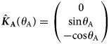


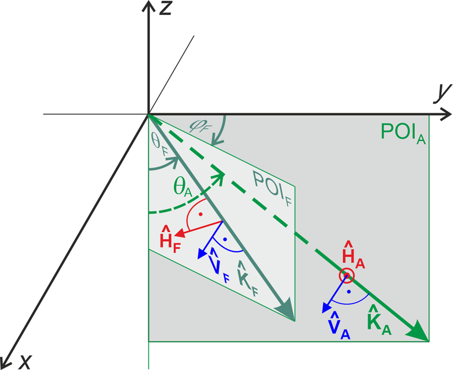
Fig. 9. Definitions of vectors and angles used in the model developed to simulate antenna temperatures from aggregated facet brightness temperatures.
Antenna unit field vectors $\hat{{\bi H}}_{\bf A} = H_{\rm A}^{{\rm H}_{\rm F}} \,\hat{{\bi H}}_{\bf F} + H_{\rm A}^{{\rm V}_{\rm F}} \,\hat{{\bi V}}_{\bf F}$ and $\hat{{\bi V}}_{\bf A} = V_{\rm A}^{{\rm V}_{\rm F}} \,\hat{{\bi V}}_{\bf F} + V_{\rm A}^{{\rm H}_{\rm F}} \,\hat{{\bi H}}_{\bf F}$
 can by expressed by Facet unit field vectors $\hat{{\bi H}}_{\bf F}$
 and $\hat{{\bi V}}_{\bf F}$
 . Components $H_{\rm A}^{{\rm H}_{\rm F}}$
 and $V_{\rm A}^{{\rm V}_{\rm F}}$
 of like-polarization and cross-polarization $H_{\rm A}^{{\rm V}_{\rm F}}$
 and $V_{\rm A}^{{\rm H}_{\rm F}}$
 are computed from scalar products (${\odot}$
 ) representing the respective orthogonal projections of Antenna polarization vectors onto the facet polarization vectors:


Accordingly, orthogonal polarized fields ${\bi E}_{\bf F}^{\bf H} = \lpar {E_{\rm F}^{\rm H} \comma \;0} \rpar$ and ${\bi E}_{\bf F}^{\bf V} = \lpar {0\comma \;E_{\rm F}^{\rm V} } \rpar$
 emitted by a single facet at θ F and φF read in the antenna reference frame:

Energy carried by an electric field is proportional to its squared field amplitude. Therefore, antenna temperatures $T_{{\rm A}\comma {\rm F}}^{\rm H}$ and $T_{{\rm A}\comma {\rm F}}^{\rm V}$
 are mixtures of brightness temperatures $T_{\rm F}^{\rm H}$
 and $T_{\rm F}^{\rm V}$
 of a single facet:
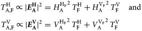
Antenna temperatures $T_{\rm A}^{\rm H}$ and $T_{\rm A}^{\rm V}$
 resulting from the collectivity of facet brightness temperatures $T_{\rm F}^{\rm H}$
 and $T_{\rm F}^{\rm V}$
 are computed as (θ F = 0°, …, 180° and φF = 0°, …, 360°):


The directional sensitivity D = D(α) of the antenna imposes weights to $T_{{\rm A}\comma {\rm F}}^{\rm H}$ and $T_{{\rm A}\comma {\rm F}}^{\rm V}$
 depending on the facet polar angle α relative to the antenna main direction. For the Pickett horn antenna (Pickett and others, Reference Pickett, Hardy and Farhoomand1984) used in our CR measurements D(α) is represented by a Gaussian model (unit of α is degree):

The polar angle α 0 for which sensitivity drops to e−1 ≃ 0.368 relative to the sensitivity D(α = 0°) = 1 along the antenna main direction was derived from time series of antenna temperatures measured with the sun passing through the antenna field of view following the approach explained in Section 3.2.1 in Schwank and others (Reference Schwank2010). The polar angle at which antenna sensitivity drops to −3 dB (to ~0.5) is α −3dB ≃ 11.5°, and the polar angle at which antenna sensitivity drops to −30 dB (to 0.001) is α −30dB ≃ 36.36°.
The polar angle α for a Facet at θ F and φF is computed from the Facet- and the Antenna unit propagation vectors:

The normalization factor N used in Eqns (A13) and (A14) is computed as (θ F = 0°, …, 180° and φF = 0°, …, 360°):
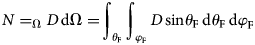
Brightness temperatures $T_{\rm F}^p \lpar {\theta_{\rm F}} \rpar$ of facets below the horizon (0° ≤ θ F ≤ 90°) are simulated with the two-layer version of LS-MEMLS (Fig. 4) considering consistent values of EM parameters. For facets above the horizon (90° < θ F ≤ 180°) $T_{\rm F}^p \lpar {\theta_{\rm F}} \rpar$
 are considered as unpolarized downwelling sky radiance T sky(θ zenith) with θ zenith = 180° − θ F being the angle between the horizon and zenith and using the model outlined in Pellarin and others (Reference Pellarin2003):


 Open access