


The first figure in Penrose (Reference Penrose1973, p. 4) is a pedigree chart of a family some of whose members had sex-linked color blindness. The chart was constructed from details in a letter written in 1777 by an affected member of the family (J. Scott), which was reproduced in transactions of the Royal Society (Scott & Lort, Reference Scott and Lort1778). The letter describes how the writer’s color vision was affected. Penrose notes that the genetic explanation of such pedigrees came almost 150 years later. Kalmus (Reference Kalmus1965) follows the tradition of the Galton Laboratory with an exposition of the diagnosis and genetics of defective color vision. Lakowski (Reference Lakowski1969, p. 177) comments: ‘congenital color defects … have been admirably discussed … by Kalmus (Reference Kalmus1965) with particular reference to the way such defects are inherited.’ Neitz and Neitz (Reference Neitz and Neitz2011) review findings from nearly half a century of more recent research. Verrelli and Tishkoff (Reference Verrelli and Tishkoff2004), Jacobs (Reference Jacobs2018), Wool et al. (Reference Wool, Packer, Zaidi and Dacey2018) and Webster (Reference Webster2020) illustrate how attempts to reach a deeper understanding of color vision have inspired and continue to motivate research on a number of fronts.
The OMIM references for the red (OPN1LW), green (OPN1MW) and blue (OPN1SW) pigment genes are, respectively, #300822, #300821 and #613522 (https://www.omim.org). Neitz and Neitz (Reference Neitz and Neitz2011, p. 5) state: ‘Protan, deutan and tritan defects are characterized by the absence of a contribution to vision from L, M and S cones, respectively’. Much of the literature on color blindness has been written without knowing the action of the genes involved.
At the time when Kalmus (Reference Kalmus1965) was writing his monograph, there was interest in the apparent fact that color blindness was relatively rare in hunter-gatherer populations compared with those supported by agriculture (Adam, Reference Adam1969; François et al., Reference François, de Bie, Verriest and Matton1972; Garth, Reference Garth1933; Junqueira et al, Reference Junqueira, Kalmus and Wishart1957; Kalmus, Reference Kalmus1957; Kalmus et al., Reference Kalmus, Amir, Levine, Barak and Goldschmidt1961, Reference Kalmus, de Garay, Rodarte and Lourdes1964; Pickford, Reference Pickford1963; Post, Reference Post1962, Reference Post1963, Reference Post1971; Salzano, Reference Salzano1961, Reference Salzano1964). It was suggested that selection against the genes connected with color vision defects was relaxed when communities began farming and genes increased in frequency by mutation. Calculations made by Kalmus (Reference Kalmus1965) can be found in his book (p. 91). Danforth (Reference Danforth1923) suggested ways of estimating mutation rates in humans. Haldane (Reference Haldane1935) was among the first to make an estimate of a mutation rate in humans, as was noted by Nachman (Reference Nachman2004). Haldane estimated the mutation rate for hemophilia to be 20 × 10–6.
François et al. (Reference François, de Bie, Verriest and Matton1972) contain a table giving the prevalence of color blindness in males recorded from a large number of studies carried out in five continents. These are summarized as simple means in Table 1. The authors note that the races more recently civilized have fewer affected males. Kalmus (Reference Kalmus1965, p. 90) bases his calculations on the assumption that, since Neolithic times, the frequency of protan genes has increased from about 0.005 to 0.02 and deutan genes from 0.016 to 0.06.
Table 1. Prevalence of color blindness in males (%)

Neel (Reference Neel, Giddins, Kaneshiro and Anderson1989) refers to research conducted by his group over the previous 20 years among the least acculturated Amerindian tribes, including the Yanomamö, then existing in South America. He describes the ‘indirect’ method of estimating mutation rates applied to a battery of proteins. The mutation rate ‘pertains to nucleotide substitutions that result in an amino acid substitution which alters either the net charge of the protein or its configuration in such a way that electrophoretic mobility is changed’ (p. 301). He arrives at the estimate of 4 × 10⁻⁵/locus per generation. Neel’s definition of mutation rate could reasonably be applied to the OPN1LW gene of Verrelli and Tishkoff (Reference Verrelli and Tishkoff2004), who report on the effect on color vision of some mutations of this gene.
Neel and Post (Reference Post1963, p. 35) suggest an alternative explanation based on some untested assumptions whose validation would require fieldwork in, say, a tribal setting. They conclude:
Should the hypothesis be validated, it would provide concrete evidence for a type of positive selection which has hitherto been largely ignored in discussions of factors to be considered in human evolution. Since colorblindness now provides the only clear example of a simply inherited defect whose frequency has significantly increased with the advent of civilization, a considerable effort directed toward exploring the correctness of this and other possible hypotheses would seem justified.
It appears that Neel did not undertake such a study, although, starting in 1966, he directed research on the Yanomamö population of the Amazonian region. In his autobiography, Neel devotes very little space to vision: he comments on the remarkable visual acuity of the Yanomamö, particularly of the men; color blindness of all types in males of tribal populations was much less common (about 2%) compared with 8% among most Caucasian groups. (Neel, Reference Neel1994, p. 151).
The main purpose of this article is to present a model of sex-linked inheritance that exhibits random variation. Kempthorne (Reference Kempthorne1957) and Crow and Kimura (Reference Crow and Kimura1970) give standard models. Simunovic (Reference Simunovic2010, Table 1, p. 749) gives the prevalence of the X-linked forms protanopia (1.01%) and deuteranopia (1.27%). We suggest that one of these could be the focus of the model given here.
This article presents a model for a trait controlled by an X-linked locus for a finite population in which the genotypes are equally fit but mutation from the ‘wild type’ to the ‘morbid’ type occurs at a constant rate. The main objective is to show how the number of individuals bearing the morbid gene vary randomly. The practical utility of the model is demonstrated by relating it to color blindness. Barker (Reference Barker1958) takes a rather different approach to simulate sex-linked selection at four stages of the life cycle of Drosophila.
Details of the model are followed by a summary of a single realization and discussion, the last giving some comments on the difficulty of testing the conjecture of Neel and Post (Reference Post1963).
The Model
Kalmus (Reference Kalmus1965, p. 59) states: ‘all the more frequent deficiencies happen to be sex-linked and usually recessive’. Schiötz (Reference Schiötz1920) has a detailed discussion, with supporting data, of the relative proportions of males and females to be expected under this mode of inheritance. Danforth (Reference Danforth1924) and von Planta (Reference von Planta1928) discuss the same topic. We consider one type controlled by a single locus and follow the numbers in the five categories: females with two ‘wild type’ alleles (
 $$\overline X$$
); females with one wild type and one ‘morbid’ gene — ‘carriers’ — heterozygotes (X); females with two morbid genes — homozygotes (H); males with a wild type gene on the X chromosome (
$$\overline X$$
); females with one wild type and one ‘morbid’ gene — ‘carriers’ — heterozygotes (X); females with two morbid genes — homozygotes (H); males with a wild type gene on the X chromosome (
 $$\overline A$$
); males with a morbid gene (A). Symbols X and so on are used to denote both the category and number of individuals in the categories.
$$\overline A$$
); males with a morbid gene (A). Symbols X and so on are used to denote both the category and number of individuals in the categories.
The gross reproductive rate in the population, expressed as number of live births of either sex per year, is denoted by r; m is the mutation rate in eggs; s the rate in sperm; and w is the proportion of a year taken up by the chosen interval of observation.
The number of both males and females is S = 10,000. Because the number is finite, simulation may lead to a chaotic outcome. This is controlled by keeping the number of males and females constant; that is,
 $$\overline X = S - (X + H)$$
and
$$\overline X = S - (X + H)$$
and
 $$\overline A = S - A.$$
We consider the pairings that produce progeny of the five types.
 $$\overline X:{p_{_{\overline X\overline A}}}(1 - m)(1 - s) + 0.5{p_{X\overline A}}(1 - m)(1 - s),$$
 $$X:{p_{\overline X\overline A}}((1 - m)s + m(1 - s)) + {p_{\overline XA}}(1 - m) + 0.5{p_{X\overline A}}(1 + m - ms) + 0.5{p_{XA}}(1 - m) + {p_{H\overline A}}(1 - s),$$
 $$H:{p_{\overline X\overline A}}ms + {p_{\overline XA}}m + 0.5{p_{X\overline A}}s + 0.5{p_{XA}}(1 + m) + {p_{H\overline A}}s + {p_{HA}},$$
 $$\overline A:{p_{\overline X}}(1 - m) + 0.5{p_X}(1 - m),$$
 $$A:{p_{\overline X}}m + 0.5{p_X}(1 + m) + {p_H}.$$
In terms (1)–(3), probabilities of couplings are given by coefficients such as
 $${p_{\overline X\overline A}}$$
, which denotes the proportion of matings producing girls when neither parent has a morbid gene. That proportion is
$${p_{\overline X\overline A}}$$
, which denotes the proportion of matings producing girls when neither parent has a morbid gene. That proportion is
 $$\overline X\overline A/{S^2}$$
, where S is both the number of males and females in the population. Similarly
$$\overline X\overline A/{S^2}$$
, where S is both the number of males and females in the population. Similarly
 $${p_{\overline X}}$$
is the proportion of females with only wild type genes, in couplings producing boys, and is
$${p_{\overline X}}$$
is the proportion of females with only wild type genes, in couplings producing boys, and is
 $$\overline X/S.$$
Changes in the population are followed in short intervals of time, in this case intervals equal to a quarter of a year, this proportion denoted by w. An arbitrary gross reproduction rate r equal to 15/1000 births of either sex per year is used. The terms in (1)–(3) are multiplied by Srw as are the terms in (4) and (5). The population is static in the sense that its total size is constant over a long period but dynamic in the sense that stochastic variation, which is stationary in the long run, occurs. Random mating is assumed. The birth and death rates are assumed to be the same in all categories, consistent with the relaxation of selection in respect of vision. Mutation is in only one direction that is normal to morbid.
Kalmus (Reference Kalmus1965) made an estimate of the coefficient of selection against color blindness, which is given on page 91 of his book. The main aim here is to illustrate how rates of mutation observed for other traits are not consistent with high levels of color blindness. One of the objectives is to study variation in the composition of the population. Variation in births and transmission of genes is produced by using the Poisson’s frequency distribution with expectations given by formulae (1)–(5). The gains from births are offset by deaths simulated using the binomial distribution with the number of ‘trials’ given by the current number in each group and the probability of death equal to the reproduction rate modified by the length of the observation interval.
An estimate of the number of males with color blindness in equilibrium can be made using formula (1). The number of carriers (X) is made equal to double the number of color-blind males (A) and trial values of A are used, together with the corresponding X and so forth, to find the number A* for which the value in (6) is closest to zero.
 $$(1 - m)(1 - s)(\overline X\overline A/S + X\overline A/(2S)) - \,\overline X.$$
Table 2 was constructed by taking S = 10,000, m = 5 × 10⁻⁵, s = 25 × 10–5 as a starting point. The mutation rates were halved, doubled and so forth, as indicated by the powers in Table 2. The logarithms of A* are plotted against the powers in Figure 1 showing an obvious linear relation.
Table 2. Estimated equilibrium number of males with color blindness


Fig. 1. Plot of the logarithm of X* against the power of the multiplier of mutation rates (S = 10,000, m = 5 × 10⁻⁵, s = 25 × 10–5).
If S, the number of males, females are doubled, halved and so forth, the values of A* are doubled, halved. Estimates of A* can be made by interpolating in a graph such as Figure 1 and taking the exponential of the resulting logarithm.
Realization
The virtual population of 20,000 individuals was followed over 15,000 years to simulate a small population but in a settled mode of existence. The initial numbers in groups are
 $$\overline X$$
= 9730, X = 268, H = 2,
$$\overline X$$
= 9730, X = 268, H = 2,
 $$\overline A$$
=9864, A = 136. These numbers were chosen because they as are close to equilibrium as is possible under the assumed mutation rates used (m = 5 × 10⁻⁵, s = 25 × 10–5). The initial numbers were obtained by trial and error to satisfy, as nearly as possible, equations (2), (3) and (5) of the previous section. Substituting in these equations yields proportions giving respective numbers 271.18, 1.89 and 136.49, hence near-stable values. The number of morbid genes in females is double the number in males at the start. Since this is a single realization, it cannot be taken to be typical of all realizations.
$$\overline A$$
=9864, A = 136. These numbers were chosen because they as are close to equilibrium as is possible under the assumed mutation rates used (m = 5 × 10⁻⁵, s = 25 × 10–5). The initial numbers were obtained by trial and error to satisfy, as nearly as possible, equations (2), (3) and (5) of the previous section. Substituting in these equations yields proportions giving respective numbers 271.18, 1.89 and 136.49, hence near-stable values. The number of morbid genes in females is double the number in males at the start. Since this is a single realization, it cannot be taken to be typical of all realizations.
The time series of the number of carriers is displayed in Figure 2, of males with color blindness in Figure 3, and of homozygous females with the morbid gene in Figure 4. Initially, 1.36% of males were color blind; the median number overall is 192 (1.92%). The median number of carriers is 376 (3.76%) and of homozygous females 4 (0.04%). Note that the median number of carriers is approximately double the number of affected males and the proportion of affected females is about the square of the proportion of affected males, as is to be expected under random mating.
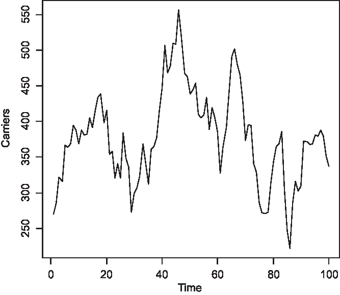
Fig. 2. Simulated number of carriers at 150 yearly intervals (S = 10,000, m = 5 × 10⁻⁵, s = 25 × 10–5).
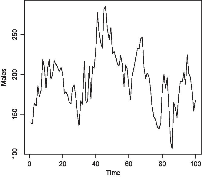
Fig. 3. Simulated number of affected males at 150 yearly intervals (S = 10,000, m = 5 × 10⁻⁵, s = 25 × 10–5).
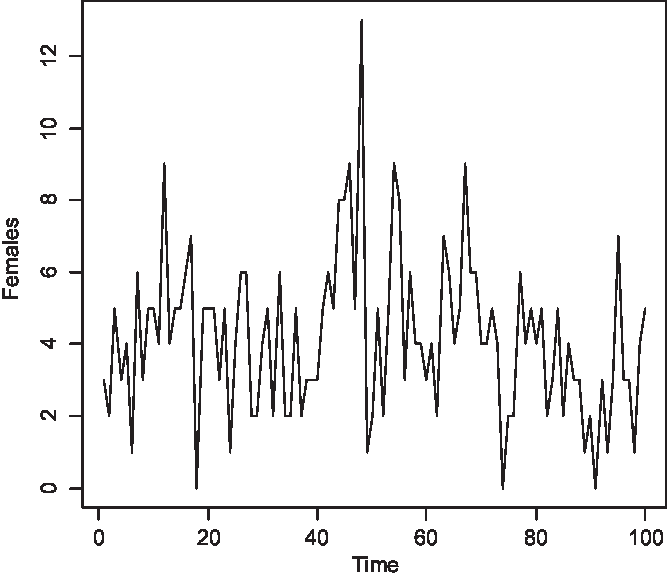
Fig. 4. Simulated number of affected females at 150 yearly intervals (S = 10,000, m = 5 × 10⁻⁵, s = 25 × 10–5).
The changes in the number of color-blind males from one observation interval to the next are given in Table 3. The difference between the mean and zero is less than 0.001, reflecting the state of statistical equilibrium. The variance of the jumps calculated from Table 2 is 1.441. The variance can be taken from the time series of A as 2 times the mean of
 $$\{ {A_t}rw(1 - rw\} ,$$
giving 1.440. The coefficient 2 is required because otherwise, the term takes account of only reductions of A due to death.
$$\{ {A_t}rw(1 - rw\} ,$$
giving 1.440. The coefficient 2 is required because otherwise, the term takes account of only reductions of A due to death.
Table 3. Simulated frequencies of changes in number of affected males from one observation interval to the next over 15,000 years

Discussion
When seeking an explanation of a difference such as that between the prevalence of color vision defects in tribal and industrialized populations, it is almost automatic to think of Darwinian selection, without specifying the details of the process.
Nei (Reference Nei1987, pp. 410−412) has a section entitled ‘Neutral Theory and Its Alternatives’, which includes the sentence: ‘Thus, if the total mutation rate per locus is v T and the fraction of deleterious mutations is f, the rate of gene substitution is given by (1 – f)v T , neglecting the effect of advantageous mutation. Here, f is related in some way to the extent of functional constraints of the gene product.’ There does not appear to be any place here for natural selection relating to a decrease or increase in the proportions of people with color vision deficiency. Nei (Reference Nei1987) does not discuss X-linked genes. Kempthorne (Reference Kempthorne1957) and Crow and Kimura (Reference Crow and Kimura1970) give a theory of selection for sex-linked genes.
The model presented here might be seen as reflecting Nei’s expression (1 – f)v T with f close to zero and v T incorporating m and s of the model; that is, proposing genes for color deficiency entering the population by mutation and leaving through death of the bearers at the same rate as the entry rate. A possible use of the model is to try various plausible mutation rates and compare the predicted prevalence of color vision deficiency with the observed values.
Color vision deficiency is not a single trait but the various forms are connected through a mosaic of photoreceptors on the retina whose inputs are processed through an elaborate communication network to the brain. The model presented here is artificial in that it imagines that part of the system can be considered in isolation. The same comment could be applied to the approach of Verrelli and Tishkoff (Reference Verrelli and Tishkoff2004).
Neel and Post (Reference Post1963) may have been thinking of the Yanomamö as a suitable population on which to test their theory on variations in the frequency of color blindness. In Homo sapiens, dubbed ‘Sapiens’ by Condemi and Savatier (Reference Condemi and Savatier2019), the eye, like other organs, is a result of hundreds of millions of years of evolution. The broad-brush approach to the evolution of Sapiens of these authors is convenient as it provides concepts and dates relevant to the Yanomamö population: Sapiens emerged in ‘hordes’ (band societies) from Africa about 100,000 years ago; ‘tribes’ (settlements) formed after (say) 60,000 years; after a further 20,000 years, Sapiens reached the New World via the Bering Strait.
Chagnon (Reference Chagnon2013) gives a detailed description of the Yanomamö tribal society. Condemi and Savatier (Reference Condemi and Savatier2019, p. 100) write: ‘a tribe is a self-governing group of humans sharing a familial origin, real (biological) or imagined (cultural, social, or legendary attribution)’.
Chagnon (Reference Chagnon2013, pp. 294−213) has a chapter entitled ‘Yanomamö Origins and Their Fertile Crescent’. At the time of his study, starting in 1965, more than 20,000 people lived in about 250 independent villages in the Amazon basin. In the view of most anthropologists, their ‘slash-and-burn’ agriculture ‘marked the transition from paleolithic hunter/gatherers to full-blown dependence on agriculture and domesticated animals’ (p. 295). Chagnon states that the Yanomamö are highly dependent on cultivated foods although ‘casual visitors’ concluded wrongly that they were hunters and gatherers. He speculates that all Yanomamö may have depended more on hunting/gathering 200 years ago.
At least, in the case of the Yanomamö, it seems that creating a simple model of a sudden transition from one form of culture to another that would have an impact on color vision adaptation is an ambitious undertaking. A reading of Chagnon (Reference Chagnon2013) shows that it would require a heroic and resourceful anthropologist to gather the necessary data. In the period when Chagnon was doing his research, the Yanomamö supported themselves with a mixture of agriculture and hunting and gathering.
Steward and Cole (Reference Steward and Cole1989) administered a questionnaire to 102 people with defective color vision and an equal number with normal color vision. Nearly 90% of dichromats and up to two-thirds of anomalous trichromats reported difficulties with everyday tasks that involve color. Nearly one-half of the trichromats reported difficulty with traffic lights and similar proportions reported color difficulties with their jobs. Substantial numbers reported that their color vision defect had affected their choice of career and many had been excluded from a chosen occupation. The subjects were patients of an optometric practice in Melbourne, Australia. It requires a stretch of the imagination to project these findings to the relative difficulties experienced by hunter-gatherers and the first farmers.
The model and the realization summarized above suggest that secular fluctuation in the frequency of a neutral or very slightly deleterious allele of an X-linked gene in a medium-to-large population is so great that a relatively high frequency is not unexpected and provides no grounds for inference about selection for color vision in human populations during the period of transition from hunter-gatherer to settled agriculture. Nor is it evidence that this period was relatively short, as has been claimed.
Acknowledgment
A referee’s comments and criticisms were used to improve the paper.


