Environmentally Driven Seasonal Forecasts of Pacific Hake Distribution

Introduction

Anticipating ecological change is an important component of living marine resource management where decisions often require lead-times of weeks to months. Yet, the lack of advanced warnings about the response of marine taxa to ecosystem shifts limits the ability of management systems to respond to rapidly changing ecosystem conditions (Clark et al., 2001; Dietze et al., 2018). Increasingly, seasonal ecological forecasts provide a means to reduce related uncertainties and play a key role in supporting management of living marine resources into the future (Hobday et al., 2016; Payne et al., 2017; Tommasi et al., 2017). Indeed, over the past decade seasonal ecological forecasts have been developed for a wide range of marine taxa including American lobster in the Gulf of Maine (Mills et al., 2017), sardines in the California Current (Zwolinski et al., 2011; Kaplan et al., 2016), and southern bluefin tuna in eastern Australia (Hobday et al., 2011a, 2016).

Increases in the predictive skill of physical ocean states has partially driven the increased availability of seasonal ecological forecasts and has resulted in the availability of skillful ocean forecasts with seasonal lead-times for many of the world’s large marine ecosystems (Stock et al., 2015; Tommasi et al., 2017; Jacox et al., 2020). In the northern California Current Ecosystem (CCE), the J-SCOPE (JISAO’s Seasonal Coastal Ocean Prediction of the Ecosystem) model provides forecasts of physical, chemical, and biological ocean states with seasonal lead times (e.g., 6–9 months) (Siedlecki et al., 2016). Skill assessments have shown the J-SCOPE model has considerable predictive skill at seasonal lead times for several ecologically relevant variables including subsurface temperature (Siedlecki et al., 2016). In turn, J-SCOPE seasonal forecasts of ocean conditions can then be used to drive ecological forecasts, such as sardine distribution in the CCE (Kaplan et al., 2016).

Pacific hake (Merluccius productus, hereafter just hake) is an important mid-trophic-level species in the CCE that supports one of the largest United States groundfish fisheries outside of Alaska (Ressler et al., 2007; Berger et al., 2019). Hake are distributed from about 25° to 55°N and at depths typically between 100 and 1000 m. The dynamics of the hake stock are characterized by episodic recruitment events with a few large age-classes dominating the stock (Hamel et al., 2015; Berger et al., 2019). Age-structure of the stock, in turn, influences distribution since older and larger hake tend to be distributed further north than smaller and younger conspecifics (Berger et al., 2019). Hake growth is variable across years and is at least partly influenced by ocean conditions (e.g., El Niño events) and availability of prey resources (Ressler et al., 2007; Hamel et al., 2015).

Pacific hake are seasonally migratory, with a northward spring migration from southern spawning grounds off the United States west coast, terminating as far north as southeast Alaska. This migration pattern results in hake being a trans-boundary resource fished commercially in the United States and Canada (Bailey et al., 1982). The fraction of the population that migrates into Canadian waters, however, can vary greatly across years, creating challenges for monitoring and management planning (Dorn, 1995). For instance, monitoring of the hake stock is conducted jointly by a United States/Canada summer acoustic-trawl survey that provides an index of hake biomass that is used for stock assessment and management planning (Berger et al., 2019). The ability of the monitoring survey to sample the full spatial extent of the stock partially determines the magnitude of uncertainty associated with the biomass index.

Environmental conditions influence the summer distribution of hake along the west coast of North America (Benson et al., 2002; Ressler et al., 2007; Agostini et al., 2008). Thermal conditions, in particular, have been positively associated with the fraction of the hake stock in Canadian waters, suggesting warmer ocean conditions drive a more northern distribution of hake (Dorn, 1995; Ware and McFarlane, 1995). More recently, evidence has suggested that thermal conditions have a spatially variable effect on hake distribution with strong positive associations with hake biomass north of Vancouver Island, British Columbia (BC) and strong negative associations offshore of Vancouver Island, BC and Washington, United States (Malick et al., 2020). This suggests that ocean temperatures could be a useful predictor of hake distribution in the northern CCE.

Skillful forecasts of hake distribution could help inform management and survey planning decisions in three important aspects. First, early warnings of changes in hake distribution can inform planning of fisheries independent surveys used to monitor the hake stock (Payne et al., 2017). For example, survey planning decisions, such as allocating survey effort between northern and southern areas, are made several months prior to the start of the survey. Thus, forecasts could inform decisions about allocating limited survey effort by predicting areas where hake are unlikely to be present in a given year. If vessel breakdowns or weather forced a reduction in survey effort, transect density could be reduced in regions predicted to have low probability of hake occurrence. Second, skillful forecasts provide information on the projected trans-boundary distribution of hake, and thus could help reduce uncertainties in the availability of the hake stock to fishers in Canada and the United States (Hobday et al., 2011b; Mills et al., 2017). Third, skillful forecasts provide early warnings of potential ecosystem shifts that can inform ecosystem-based management (Levin et al., 2009; Malick et al., 2017). For instance, Pacific hake are an important predator of fish and shellfish populations and are prey for larger fish and marine mammals in the CCE, thus advanced warnings of shifts in hake distribution could aid detection of consequential ecological shifts in the CCE (Bailey et al., 1982; Francis, 1983).

In this study, we examined whether seasonal forecasts of physical oceanographic conditions can be used to accurately predict hake distribution in the northern CCE. In particular, we developed and tested 8-month lead-time forecasts of summer hake distribution with the goal of providing forecasts to support management and survey planning decisions. We used 7 years of acoustic-trawl survey data to characterize hake distribution. We then used the J-SCOPE regional ocean model to develop 8-month lead-time forecasts of subsurface temperatures that were used to force environmentally driven species distribution models for hake. We further evaluated whether multi-model ensembles improved forecast skill of hake distribution by comparing ensemble forecasts to single-model forecasts. This process of using oceanographic forecasts to predict hake distributional shifts in the CCE explicitly addresses fisheries management ecosystem-linkage goals and provides necessary context for short-term oceanographic variability within the scope of longer-term perturbations (e.g., climate change).

Materials and Methods

The primary motivation for developing seasonal forecasts of hake distribution was to provide an early warning of changes in hake distribution to support management decisions and Pacific hake acoustic-trawl survey planning. As a result, forecasts were co-developed with survey planners, while stakeholder involvement occurred via meetings associated with the Pacific hake treaty process.

Pacific Hake Data

The hake survey aims to sample the full range of the hake distribution in summer, and survey extent and the number of transects are often adjusted in response to the presence or absence of hake following survey design guidelines. Therefore, we focus on forecasting the probability of hake occurrence, rather than density, because the acoustic-trawl survey is better informed by early warnings in the expansion or contraction of hake distribution than forecasts of hake density in a given location.

We used 7 years of spatially explicit biennial hake occurrence data collected via joint United States/Canada acoustic-trawl surveys from 2009 to 2019, with an additional 2012 survey (Table 1). Surveys started in southern California and moved northward along the United States and Canada west coasts until hake were no longer observed (typically around 54.5°N). The spatial extent of data analyzed here, however, was limited to the region 43–50°N – the latitudinal domain of the J-SCOPE model used to generate forecasts of ocean conditions (see below). The number of annual survey transects within the study domain ranged from 34 in 2015 to 49 in 2011 (Table 1). Survey timing was fairly consistent across years, with the southern third of the study domain typically sampled during the second half of July and the northern two-thirds typically sampled during August.

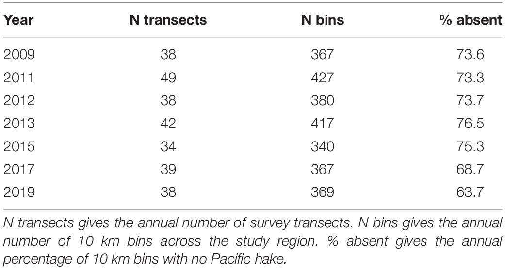
Table 1. Summary of acoustic-trawl survey data available for analysis.

Acoustic backscatter measurements attributable to hake were converted to hake biomass using the procedures outlined in Fleischer et al. (2008) and Malick et al. (2020). We aggregated the hake data into 10 km bins to reduce spatial autocorrelation in the data and coded bins with non-zero biomass as hake occurrences. We also tested smaller (e.g., 5 km) and larger (e.g., 20 km) bin sizes and found results were robust across different sized bins.

Ocean Forecasts

We used 8-month lead-time forecasts of temperature at 250 m depth from J-SCOPE to forecast hake distribution (Supplementary Figure S1). J-SCOPE is a Regional Ocean Modeling System (ROMS) (Haidvogel et al., 2008) simulation of seasonal ocean conditions spanning 43–50°N on the outer coast of Washington, Oregon, and southern BC (Siedlecki et al., 2016). The J-SCOPE model has a 1.5 km horizontal resolution with 40 vertical levels and includes both rivers and tides. The large scale oceanic and atmospheric forcing comes from NOAA’s global Climate Forecast System (CFS). In this study, we focus on retrospective ocean forecasts, i.e., reforecasts, which are true forecasts for a historical period using a free-running model unconstrained by observations after initialization. The aim in using these reforecasts was to test the models skill for jointly predicting future ocean conditions and hake distribution 8-months ahead.

We chose temperature at 250 m depth as our primary ocean variable because (1) previous research has shown strong correlations between temperature at depth and hake distribution (Malick et al., 2020), and (2) 250 m represents depths commonly occupied by hake (Ressler et al., 2007). In areas where bottom depth was less than 250 m, we used bottom temperature instead. July and August temperature forecasts were generated for each survey year using a January initialization period. For 2019, three model runs from CFS were used to quantify the uncertainty related to those forcing variables. The model runs were chosen from the beginning (January 5), middle (January 15), and end (January 25) of the forecast initialization month. The initial conditions for J-SCOPE ROMS consist of the average conditions from CFS-reanalysis for the initialization month of the forecast. As is typical in the oceanographic literature, we focus on anomalies – i.e., differences from the climatology or time-averaged field detailing the seasonal cycle. In this case, the J-SCOPE reforecast climatology was based on 2009–2017, building on Siedlecki et al. (2016).

In addition to the dynamic temperature variable, we also explored a static index of cross-shelf location as a predictor of hake distribution. In particular, we used the distance to the 200 m shelf break, where the distance was defined as the minimum euclidean distance between a hake observation and the 200 m isobath. Positive values of the shelf distance variable indicated the hake observation was offshore of the 200 m isobath and negative values indicated the observation was inshore.

Statistical Forecasting Models

We used both generalized additive models (GAM) and boosted regression trees (BRT) to model species distribution, because previous studies have shown the potential for differences in explanatory power and predictive skill across model types (Abrahms et al., 2019; Brodie et al., 2019).

We used binomial GAMs with a logit link to predict the probability of hake occurrence,

where y is the logit transformed probability of occurrence for year t at location i, α is the intercept, s is a univariate smooth function of shelf break distance (S), f is a smooth function that describes the effect of temperature anomaly at 250 m depth (T; i.e., deviations from the long-term mean), and ϵ_t,i are model residuals.

We considered two alternative formulations for the f temperature term (Table 2). The first formulation assumed a spatially stationary temperature effect modeled as a univariate smooth function of temperature, s(T_t,i). The second formulation allowed for a spatially variable temperature effect by modeling the temperature effect as the product of T_t,i and a bivariate smooth function of longitude (lon) and latitude (lat), i.e., g(lon,lat)⋅T_t,i. Non-parametric thin plate regression splines were used for the univariate (s) and bivariate (g) smooth functions in the GAMs (Wood, 2003).

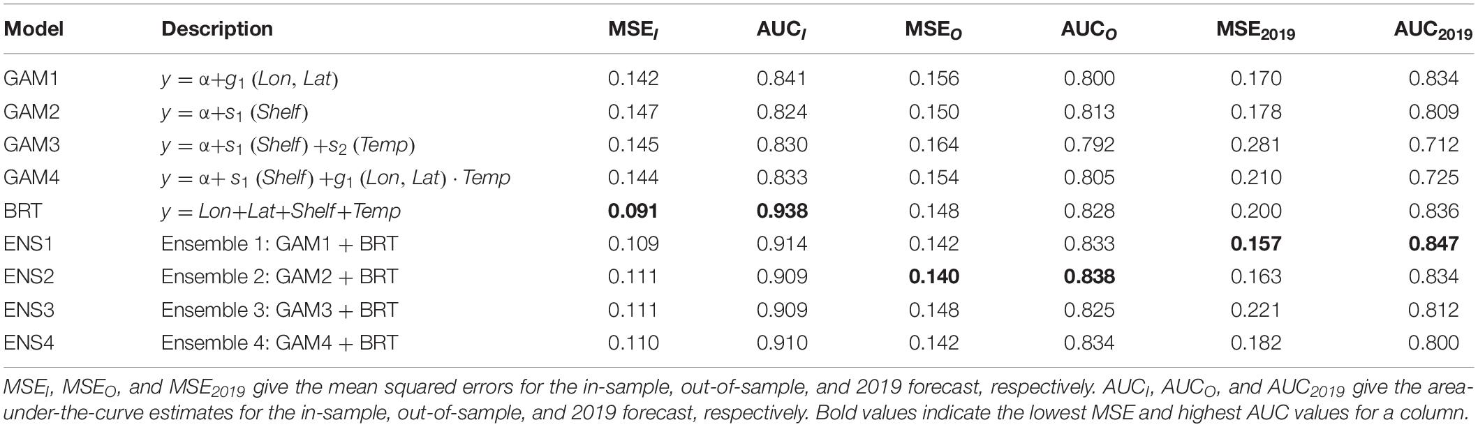
Table 2. Summary of forecast model performance.

Two simpler GAMs that included static covariates were considered as alternative null forecast models (Table 2). The first simpler model included a univariate smooth of shelf break distance. The second simpler model included a bivariate smooth of longitude and latitude. In total, we evaluated four alternative GAM forecast models (Table 2).

The BRT used a Bernoulli distribution. Since BRT models can handle colinearity among predictors, we included four covariates: temperature anomaly at 250 m depth, distance to the shelf break, longitude, and latitude (Elith et al., 2008). BRT models are composed of a large number of decision trees constructed via recursive binary splits of the data with non-linear responses produced by evaluating these splits across many trees (Elith et al., 2008). The BRT was estimated using a maximum of three interactions among covariates, a learning rate of 0.02, and bag fraction of 0.6, which resulted in models with at least 1000 trees (Elith et al., 2008). Standard errors of predicted species distribution were calculated across 100 BRT fits to provide model error estimates (Hazen et al., 2018; Brodie et al., 2019).

Four ensemble model forecasts were generated by averaging each of the GAMs and the BRT, where each model in the ensemble was given equal weight (Clemen, 1989; Araujo and New, 2007). We also tested the sensitivity of our results to the inclusion of temperature in the BRT by re-running the analysis with temperature anomaly at 250 m excluded from the BRT model. All analyses were conducted using R v3.6.0 and the mgcv and dismo packages (Elith et al., 2008; Wood, 2017; R Core Team, 2019).

Forecast Evaluation

Previous work has shown considerable skill for the J-SCOPE temperature forecast model. Siedlecki et al. (2016) evaluated J-SCOPE’s predictability for temperature, and found that predictive skill increased with depth. In addition, annual evaluation of J-SCOPE forecasts against observations are available on the NANOOS IOOS portal¹. Supplementing earlier evaluations of J-SCOPE performance and skill, we further quantified performance of J-SCOPE predictions of bottom temperature by comparing against temperature data from the Northwest Fisheries Science Center’s West Coast Groundfish Bottom Trawl Survey (Keller et al., 2017). That survey samples the United States West Coast slope and shelf (55–1280 m) annually from May-October, targeting bottom-dwelling species of commercial importance.

We evaluated the GAM and BRT model performance using a combination of in-sample and out-of-sample metrics including the area-under-the-curve (AUC) and mean squared error (MSE) (Fielding and Bell, 1997). The AUC measures how well a model can discriminate a presence from an absence. The AUC ranges between 0 and 1 where a value of 0.5 indicates a random classifier and values closer to 1 indicate higher forecast skill. The MSE measures the accuracy of the forecast model where lower values indicate a more accurate forecast.

We used leave-one-year-out cross validation to evaluate how the models performed at forecasting hake distribution for un-observed years (Fielding and Bell, 1997). In this procedure, a single year was left-out of the data, each model was re-fit using the remaining years of data, and forecasts were produced for the left-out year. This cross-validation was repeated for each year, providing 7 years of out-of-sample forecasts. We then compared the forecasted values for the left-out years to the observed values using the MSE and AUC metrics.

To further test the performance of the forecast models, we generated “true” out-of-sample forecasts for 2019 prior to the hake acoustic-trawl survey. We fit the hake forecast models using data through 2017 and then tested those models using true forecasts of the physical environment from the J-SCOPE January initialized temperature forecasts. True forecasts are produced every January and released on the web in February prior to the conditions being observed, thus referred to as a “true” forecast. In this case, J-SCOPE ocean forecasts were used to generate forecasts of hake distribution for August 2019. To better characterize uncertainty in the ocean forecasts, we generated three forecasts from the J-SCOPE model for 2019 using different initialization dates in January (January 5, January 15, January 25). The spread across the three forecasts was used as a measure of uncertainty in the J-SCOPE temperature forecasts. For each hake forecasting model, we generated separate forecasts for each of the three temperature forecasts and used an average across the three forecasts as our ensemble mean 2019 hake forecast for each model. Performance of the 2019 hake forecasts was evaluated using the AUC and MSE metrics.

Results

J-SCOPE performed well when bottom temperatures observed in situ were compared with the simulated bottom temperatures from the same locations (R² = 0.88; Supplementary Figure S2). The predicted bottom temperatures were biased warm (RMSE = 0.48), which is not uncommon in ROMS applications and is addressed here by focusing on anomalies rather than raw temperature values (Giddings et al., 2014). This strong agreement between observed and predicted temperatures supports the use of numerical ocean model forecasts of sub-surface temperatures to predict suitable hake habitat.

Hake occurred across the latitudinal extent of the study region with the exception of 2011, when no fish were observed off the west coast of Vancouver Island (Figure 1). Across all years, the cross-shelf distribution of hake was concentrated around the 200 m isobath with the majority of hake occurrences (62%) occurring within 10 km of the shelf break (Figure 1). The percentage of hake absences across years was consistent ranging from 64% in 2019 to 77% in 2013, although the latitudinal distribution of absences varied across years (Table 1). For example, in 2015 hake were absent from most locations off-shore of Washington and Oregon, whereas in 2011 hake occurrences tended to be concentrated in this region (Figure 1).

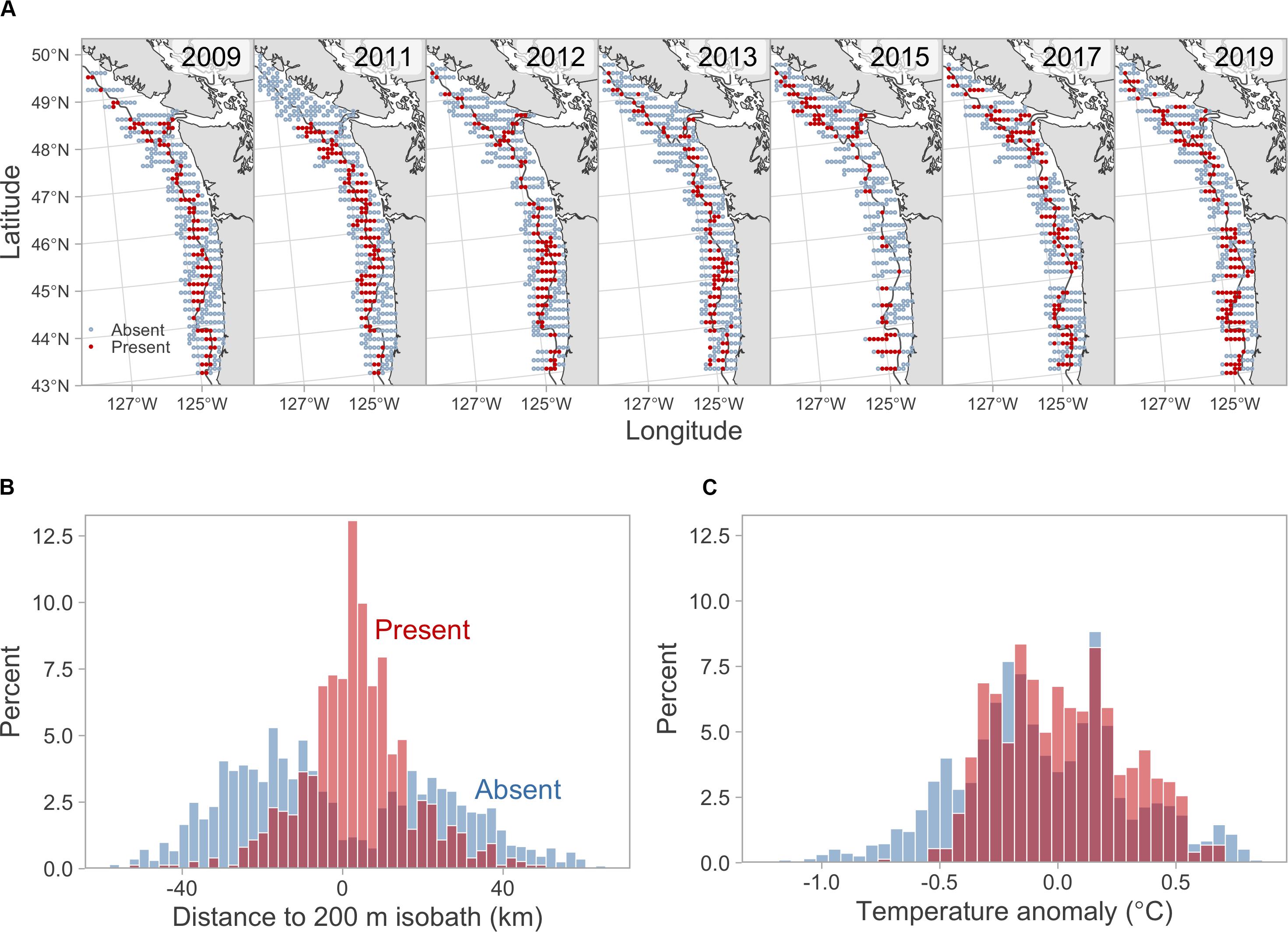
Figure 1. Pacific hake summer distribution as determined by acoustic-trawl surveys. (A) Annual occurrences and absences of Pacific hake across the study region. Solid red circles indicate hake occurrences and open blue circles indicate hake absences. Solid gray lines show the 200 m isobath. (B) Histograms of distance to the 200 m isobath for Pacific hake occurrences (red) and absences (blue). Darker red bars indicate overlap between the occurrences and absences. (C) Histograms of temperature anomaly at 250 m depth for Pacific hake occurrences (red) and absences (blue). Temperature anomalies are reforecasts from the J-SCOPE model.

The shelf-break term in the GAM and BRT models confirmed the strong preference of hake to be present slightly offshore of the 200 m shelf-break (Figures 2A, 3A–C). The shelf-break preference was also the dominant pattern in the bivariate smooth of longitude and latitude in model GAM1 (Figure 2B). The stationary temperature terms in the GAM3 and BRT models indicated that hake occurrence tended to have a positive association with temperature anomaly (Figures 2C, 3D). In contrast, the non-stationary temperature term in model GAM4 showed negative associations between temperature and hake occurrence off the Washington and Oregon coasts, but positive associations in more northern and southern areas (Figure 2D).

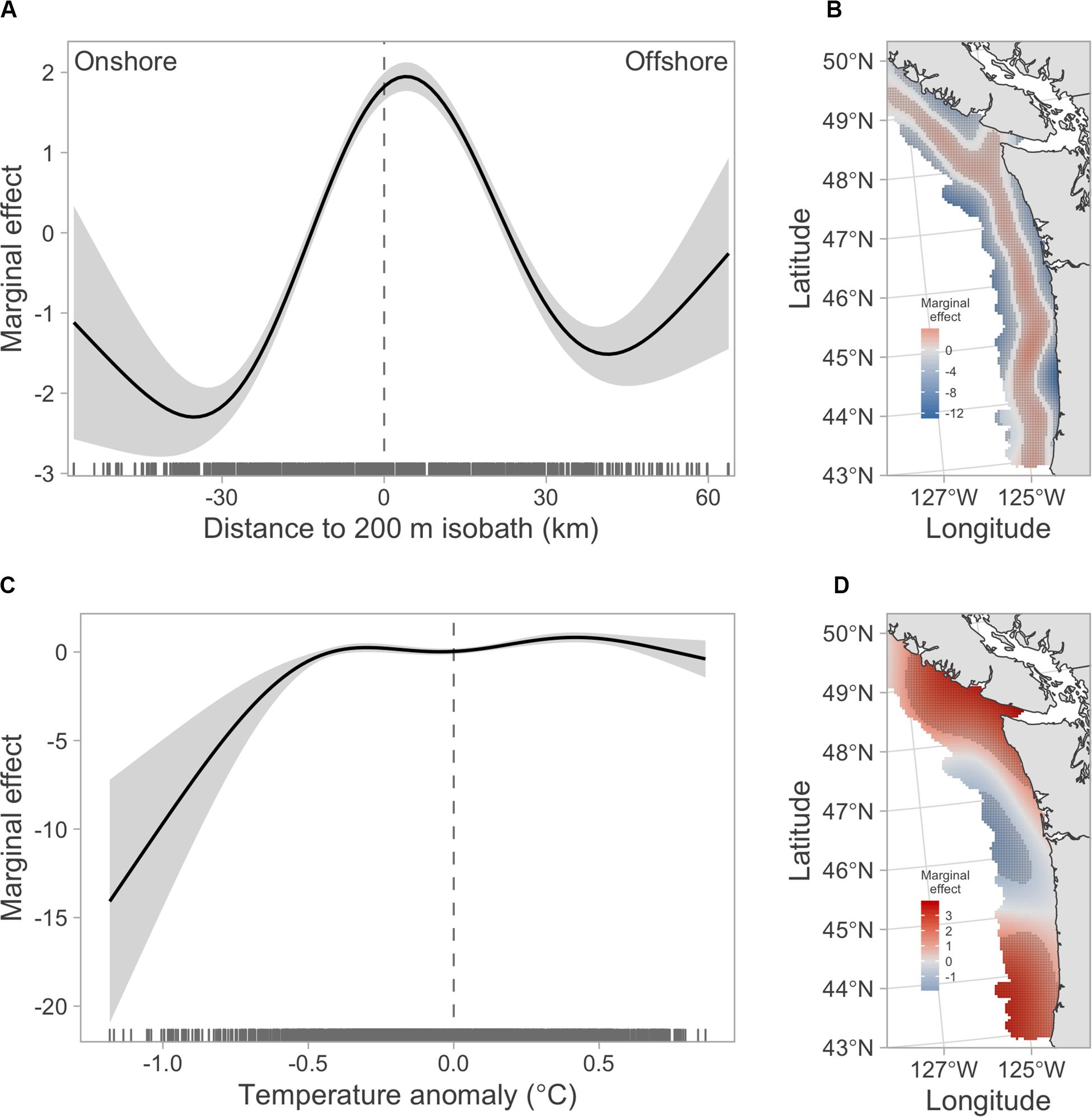
Figure 2. Marginal effects of covariate smooths from the GAMs. (A) Marginal effect of shelf break term in model GAM2. (B) Marginal effect of bivariate longitude–latitude term in model GAM1. (C) Marginal effect of stationary temperature anomaly term in model GAM3. (D) Marginal effect of spatially non-stationary temperature anomaly term in model GAM4. In panels (A,C), gray shaded regions show 95% confidence intervals. In panels (B,D), stippling indicates location where the 95% confidence interval for the covariate effect does not include zero.

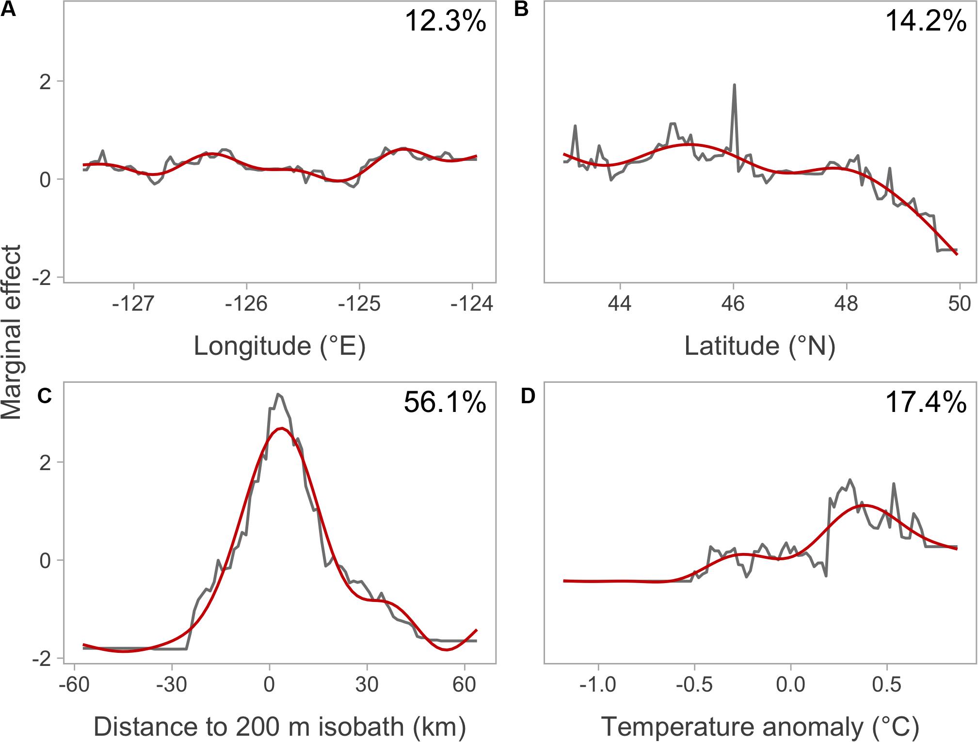
Figure 3. Marginal effects of covariate smooths from the BRT. Each panel shows a single covariate: (A) longitude, (B) latitude, (C) distance to 200 m isobath, and (D) temperature anomaly. Gray lines show the marginal effects and red lines show smoothed marginal effects. Percentages give relative influence (i.e., percentage contribution) of each variable in explaining model deviance.

All forecasting models had considerable forecast skill (both in-sample and out-of-sample) with AUC values greater than 0.79 and MSE values lower than 0.17 (Table 2). The BRT tended to fit the data the best with the highest in-sample AUC (0.93) and lowest in-sample MSE (0.09). For out-of-sample, however, an ensemble model (ENS2) performed best with an overall AUC of 0.84 and MSE of 0.14 (Table 2). Among the four GAMs, the longitude-latitude model (GAM1) tended to fit the data the best (i.e., had the highest AUC and lowest MSE), whereas the shelf-only model (GAM2) had the best out-of-sample forecast skill (Table 2). Between the two GAMs that included a temperature effect (GAM3 and GAM4), there was support for a spatially varying temperature effect with the GAM4 model having better in-sample and out-of-sample performance than GAM2.

The 2019 temperature anomaly forecasts from the J-SCOPE model indicated above average temperatures at depth across the study region (Figure 4A) with the warmest forecast (Figure 4C) having an average temperature anomaly of 0.78°C and the coolest forecast (Figure 4B) having an average anomaly of 0.36°C. The three individual temperature forecasts displayed moderate variability in temperature anomalies with grid cell specific standard deviations across the three temperature forecasts ranging from 0.03 to 1.36 (Supplementary Figure S3).

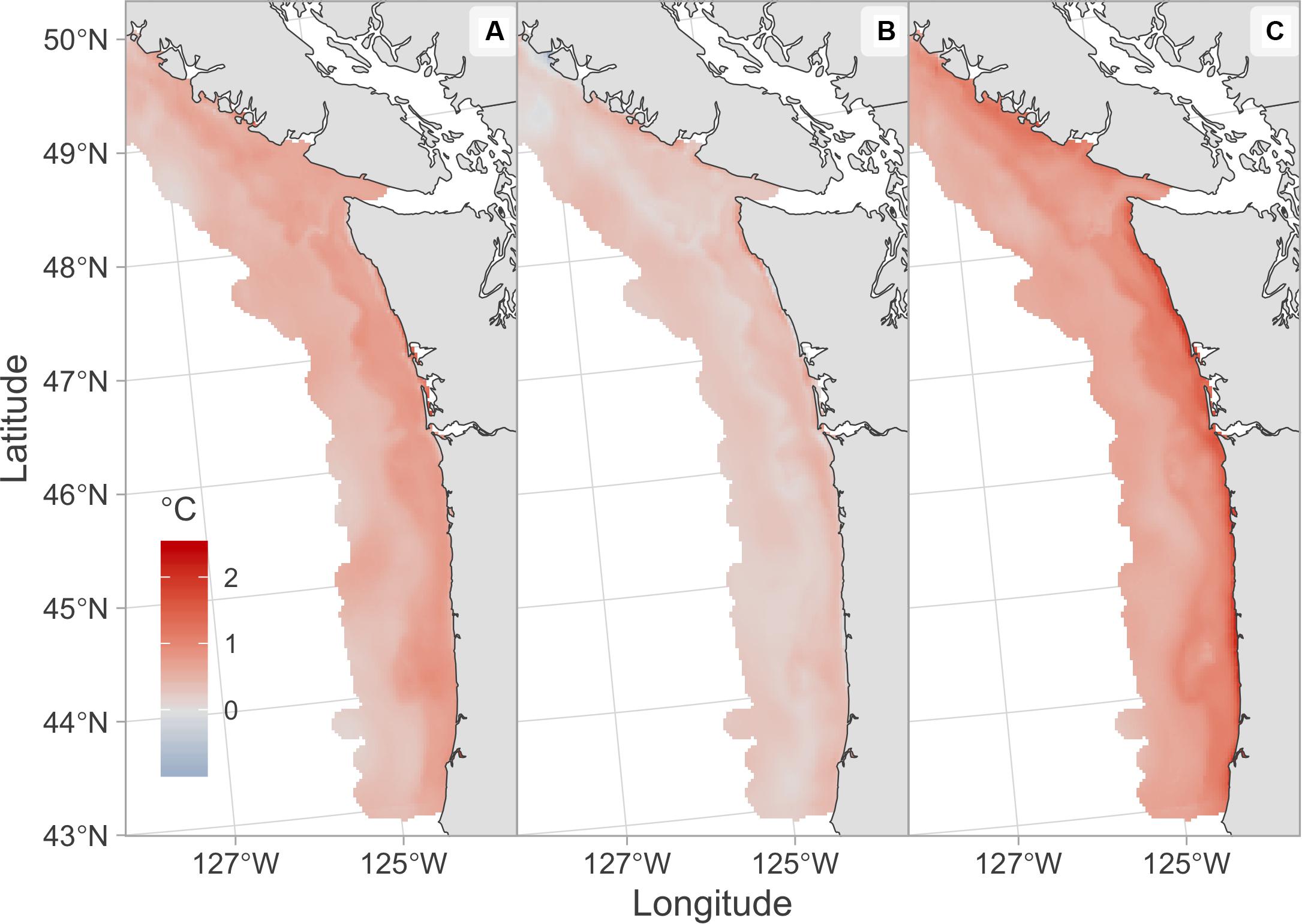
Figure 4. January initialized August 2019 forecasts of temperature anomaly at 250 m depth from the J-SCOPE model. Each panel shows an alternative temperature forecast initialized on different days; (A) January 5, (B) January 15, (C) January 25.

All models had considerable skill in forecasting 2019 hake occurrence with the ENS1 model having the best 2019 forecast skill with an AUC of 0.85 and MSE of 0.16 (Table 2 and Figure 5). The 2019 forecasts showed higher probabilities of hake occurrence near the 200 m isobath, which is consistent with their historical distribution within the study region. The three models that included temperature anomaly (GAM3, GAM4, and BRT) showed more spatial variability in predicted hake occurrence and also tended to have higher standard errors of prediction compared to models that lacked temperature (Figures 5, 6).

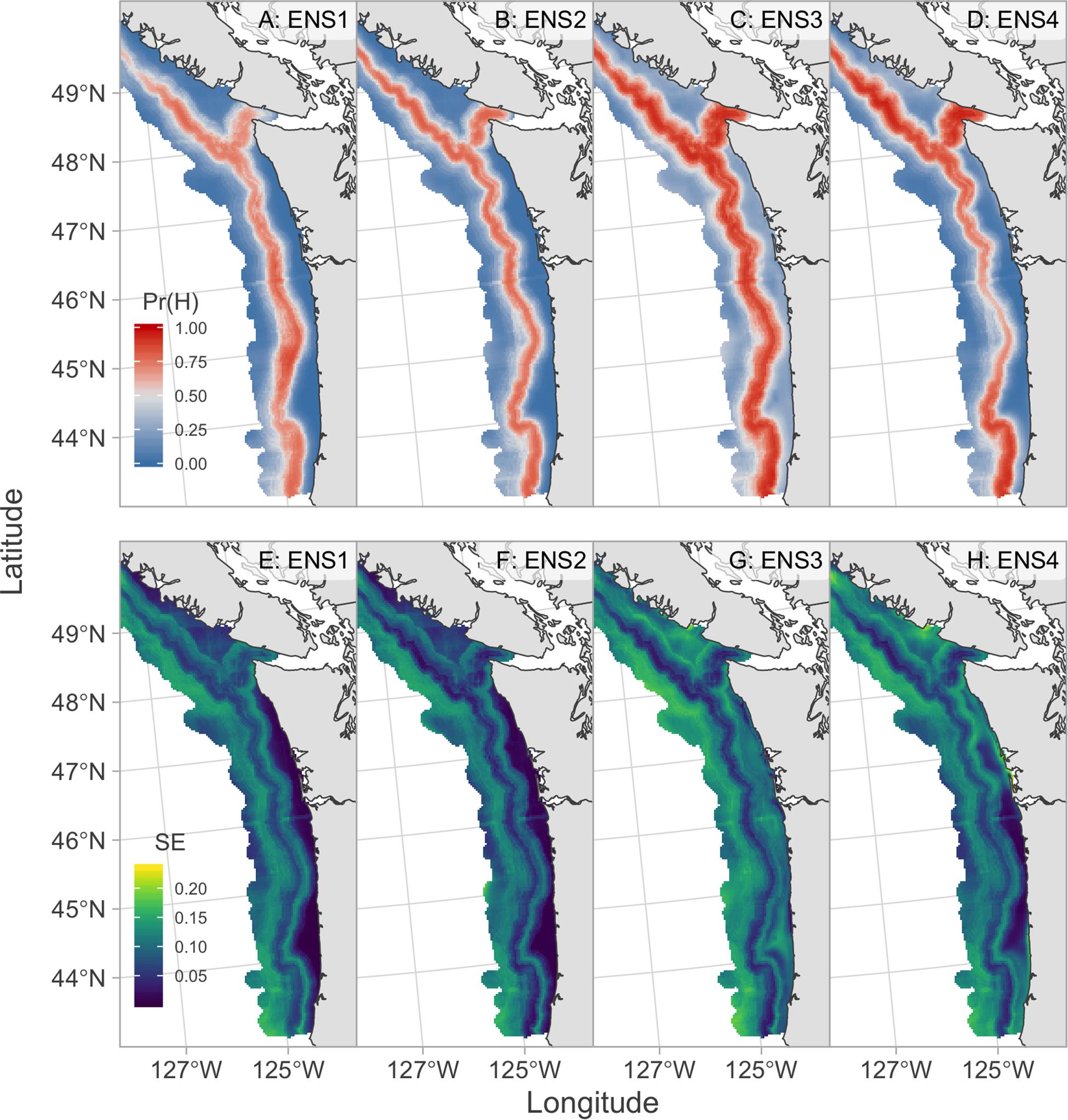
Figure 5. August 2019 forecasts of hake occurrence from ensemble forecast models. Top row (A–D) shows the probability of hake occurrence where red indicates probabilities greater than 0.5 and blue indicates probabilities less than 0.5. Bottom row (E–H) shows the associated standard errors for each model where brighter colors indicate higher forecast uncertainty.

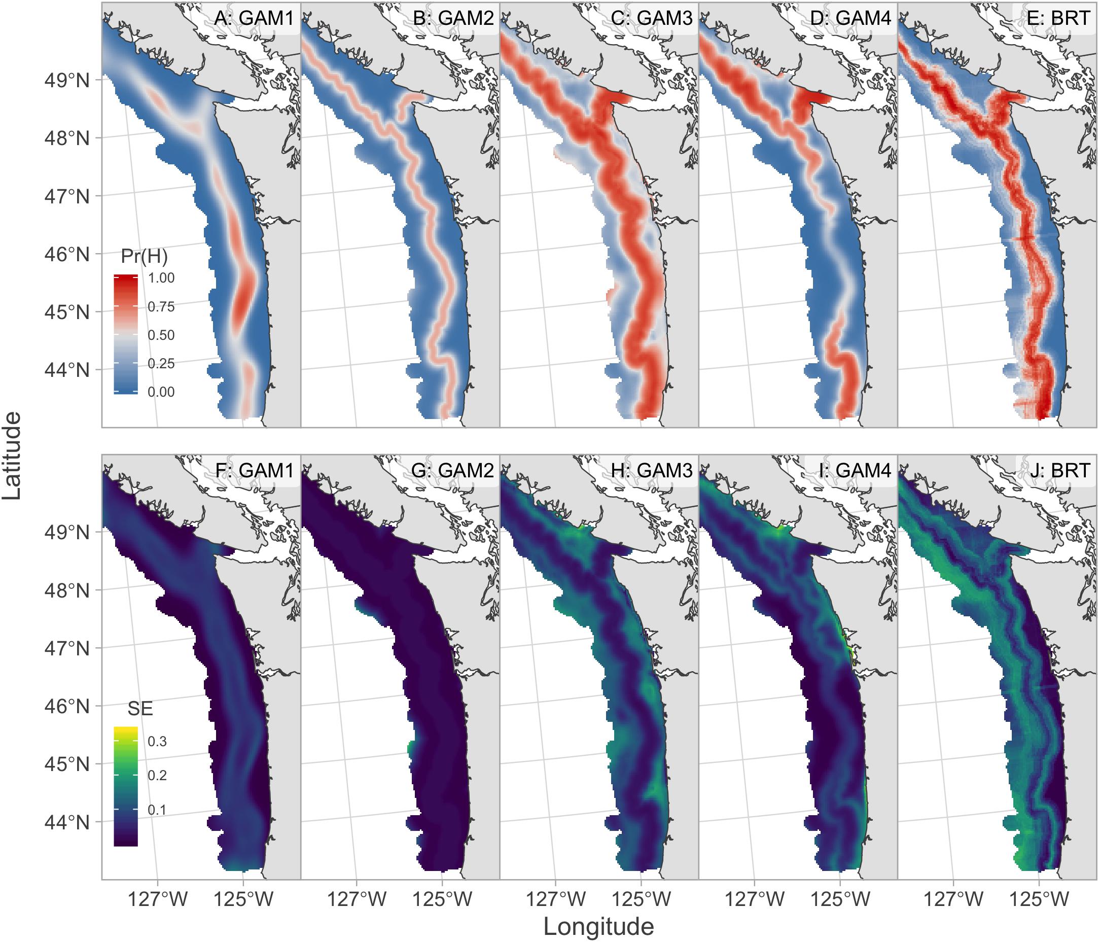
Figure 6. August 2019 forecasts of hake occurrence from individual forecast models. Top row (A–E) shows the probability of hake occurrence where red indicates probabilities greater than 0.5 and blue indicates probabilities less than 0.5. Bottom row (F–J) shows the associated standard errors for each model where brighter colors indicate higher forecast uncertainty.

When temperature was removed from the BRT, model fit declined compared to the original BRT model that included temperature (i.e., lower in-sample skill; Table 2 and Supplementary Table S1). In addition, the model with the highest out-of-sample skill changed to an ensemble of the BRT without temperature and GAM4, which includes a non-stationary temperature effect, suggesting temperature contributes to out-of-sample forecast skill.

Discussion

Our objective was to develop and test environmentally driven seasonal forecasts of hake distribution to support management and survey planning decisions. The forecast models we tested showed appreciable out-of-sample forecast skill at 8-month time horizons. In addition, we found that: (1) the J-SCOPE model had considerable predictive skill of subsurface temperatures throughout the study domain, (2) distance to the 200 m shelf break was a strong predictor of historical hake occurrence and temperature at depth had a spatially varying effect on the probability of occurrence; and (3) the BRT model had moderately higher forecast skill than the GAMs and a multi-model ensemble forecast had slightly better out-of-sample forecast skill compared to the individual GAM and BRT models. Together, our results suggest that comparatively simple models can forecast hake distribution using seasonal projections of subsurface ocean temperature and distance to the 200 m shelf break.

Most of the forecast skill was derived from the 200 m shelf-break covariate. The strong affinity for hake occurrences to be concentrated in areas just-offshore of the 200 m shelf break is consistent with several previous studies that have shown areas near the 200 m isobath and areas with steeply sloping bathymetry provide good hake habitat (Dorn, 1995; Mackas et al., 1997; Swartzman, 1997, 2001). One possible explanation for this is that food availability may be high in these areas. In particular, euphausiids – an important prey item for hake – tend to concentrate in areas of steeply sloping bathymetry and submarine canyons (Buckley and Livingston, 1997; Mackas et al., 1997; Santora et al., 2018). In addition, areas just offshore of the 200 m isobath may also provide good physical ocean conditions. For instance, the California Undercurrent is strongest offshore of the 200 m isobath; the northward flowing undercurrent may act as a migration corridor for hake that could facilitate northward migration of Pacific hake and aggregate prey resources (Bakun, 1996; Agostini et al., 2006).

Our results indicated a moderate subsurface temperature effect on hake occurrence. The best GAMs included a spatially variable temperature effect and the BRT indicated the temperature term accounted for ∼17% of the variability in the response. This result broadly agrees with several previous papers that have shown associations between hake and temperature at depth (Ressler et al., 2007; Hamel et al., 2015; Malick et al., 2020). Temperature most likely acts as a proxy for other processes that have a more direct impact on hake distribution because the temperature ranges analyzed here are comparable to previously observed in situ temperature preferences of hake (Bailey et al., 1982; Ressler et al., 2007). Although using variables that have a more direct impact on hake habitat preferences (e.g., food availability) may provide better forecasts, skillful forecast of lower-trophic-level processes relevant for hake (e.g., euphausiid distribution) are currently not available. In contrast, temperature provides an ecologically relevant variable for which there is forecast skill at the lead-times important for decision makers (Kaplan et al., 2016; Siedlecki et al., 2016; Jacox et al., 2017).

The nine forecasting models evaluated here (five individual models + four ensemble models) performed similarly across years when forecasting out-of-sample hake distribution, e.g., most forecasts for 2011 and 2017 had relatively low skill, whereas forecasts for 2009 and 2012 had relatively high skill (Supplementary Figures S4, S5). Two factors likely contributed to lower forecast skill in some years. First, gaps in the latitudinal distribution of hake reduced skill, which occurred in 2011 when hake stock size was lower and few were present off the west coast of Vancouver Island. Second, variability in the cross-shelf distribution also appears to reduce skill; in 2017, hake occurrences were concentrated just inshore of the 200 m isobath, but just offshore in all other years (Figure 1 and Supplementary Figure S6). This suggests that the consistency in which hake are present just offshore of the 200 m isobath across the latitudinal range of the study area drives differences in forecast skill among years. A priority for future research would be to examine additional covariates to better capture inter-annual deviations in distribution from the shelf-break, e.g., the California Undercurrent or subsurface oxygen concentrations.

Combining multiple forecasts into an ensemble forecast has been widely shown to produce increased forecast precision compared to individual model forecasts, given that the individual forecasts provide some independent information (Bates and Granger, 1969; Clemen, 1989; Abrahms et al., 2019). We found that the ensemble hake forecasts had only slightly better out-of-sample skill compared to the individual model forecasts (Table 2). The weak increase in predictive performance for the ensemble models compared to the individual GAM and BRT models is likely due to high correlations among model prediction errors. Multi-model ensemble models tend to outperform individual model predictions when weakly or negatively correlated model predictions are combined due to cancelation of random errors (Clemen, 1989). In this study, however, the individual model forecast error (i.e., observed hake occurrence - forecasted probability of occurrence), were strongly correlated, e.g., the average pairwise correlation of forecast errors from the GAMs and BRT was 0.91 (Supplementary Figure S7). This indicates that the individual forecast models produce similar forecast errors, which reduces the effectiveness of multi-model averaging (Araujo and New, 2007).

The results presented here provide a critical first step in developing an early warning of hake distributional shifts. Yet, we believe future work on three areas could further improve the usefulness of hake forecasts for management and survey planning. First, extending the northern range of this work to include waters through SE Alaska could help inform survey planning by providing additional information on the projected northern extent of Pacific hake, which is a critical uncertainty during survey planning. Second, developing a forecast of hake density could improve how the forecasts inform management decisions by helping to reduce uncertainties regarding the proportion of the population expected to migrate into Canadian waters. Third, if the spatial extent of the study area is extended northward beyond 50°N, the maximum latitudinal domain of this study, accounting for impacts of age-structure on Pacific hake distribution may be important. Exploratory analysis did not identify strong age-based differences in Pacific hake occurrences within the current spatial extent; however, evidence suggests that older and larger hake tend to migrate further north than smaller hake with few age-2 hake observed north of Vancouver Island (Ressler et al., 2007; Malick et al., 2020).

Collectively, our results provide evidence that hake distribution can be skillfully forecast at lead-times of 8-months in the northern CCE. Our results also illustrate the broader utility of using seasonal lead-time ocean predictions in an ecological context to provide early warnings of distribution shifts of ecologically and economically important marine species. Marine ecosystems are changing rapidly and experiencing extreme events more frequently. Thus, skillful ecological forecasts provide new tools to inform the management process by reducing uncertainties regarding future states of nature that management decisions are often dependent upon (Dietze et al., 2018).

Data Availability Statement

The raw data supporting the conclusions of this article will be made available by the authors, without undue reservation.

Author Contributions

MM was the principal author of the manuscript and led the modeling analysis. MM, MH, SP-S, SS, IK, MH, KM, and AB designed the study and contributed to interpreting the results. SP-S and SG performed the data collection and processing. SS, EM, AH, and NB ran the J-SCOPE model forecasts and conducted the skill analysis. All authors contributed to writing and editing of the manuscript.

Funding

Funding was provided by NOAA’s Fisheries and the Environment (FATE) program (grant #16-08). This study was partially supported by NOAA’s Climate Program Office’s Modeling, Analysis, Predictions, and Projections Program, Grant #NA17OAR4310112. This publication is partially funded by the Joint Institute for the Study of the Atmosphere and Ocean (JISAO) under NOAA Cooperative Agreement NA15OAR4320063, Contribution No. 2018-0183. The J-SCOPE forecasts were performed on the University of Washington Hyak supercomputer system, supported in part by the University of Washington eScience Institute.

Conflict of Interest

The authors declare that the research was conducted in the absence of any commercial or financial relationships that could be construed as a potential conflict of interest.

Acknowledgments

We thank Rebecca Thomas, Dezhang Chu, and John Pohl for assistance with the hake biomass data, as well as for helpful discussions that improved this study. We also thank Lewis Barnett and Nick Tolimieri for useful comments on our manuscript. We are grateful to the captains and crew members of the vessels used to conduct the acoustic-trawl surveys.

Supplementary Material

The Supplementary Material for this article can be found online at: https://www.frontiersin.org/articles/10.3389/fmars.2020.578490/full#supplementary-material

Footnotes

1. ^ http://www.nanoos.org/products/j-scope/home.php

References

Abrahms, B., Welch, H., Brodie, S., Jacox, M. G., Becker, E. A., Bograd, S. J., et al. (2019). Dynamic ensemble models to predict distributions and anthropogenic risk exposure for highly mobile species. Divers. Distrib. 25, 1182–1193. doi: 10.1111/ddi.12940
Agostini, V. N., Francis, R. C., Hollowed, A. B., Pierce, S. D., Wilson, C., and Hendrix, A. N. (2006). The relationship between Pacific hake (Merluccius productus) distribution and poleward subsurface flow in the California current system. Can. J. Fish. Aquat. Sci. 63, 2648–2659. doi: 10.1139/f06-139
Agostini, V. N., Hendrix, A. N., Hollowed, A. B., Wilson, C. D., Pierce, S. D., and Francis, R. C. (2008). Climate–ocean variability and Pacific hake: a geostatistical modeling approach. J. Mar. Syst. 71, 237–248. doi: 10.1016/j.jmarsys.2007.01.010
Araujo, M., and New, M. (2007). Ensemble forecasting of species distributions. Trends Ecol. Evol. 22, 42–47. doi: 10.1016/j.tree.2006.09.010
Bailey, K. M., Francis, R. C., and Stevens, P. R. (1982). The life history and fishery of Pacific whiting, Merluccius productus. Cal. Coop. Ocean Fish. 23, 81–98.
Bakun, A. (1996). Patterns in the Ocean: Ocean Processes and Marine Population Dynamics. La Paz: California Sea Grant College System.
Bates, J. M., and Granger, C. W. J. (1969). The combination of forecasts. Oper. Res. Q. 20, 451–468. doi: 10.2307/3008764
Benson, A. J., McFarlane, G. A., Allen, S. E., and Dower, J. F. (2002). Changes in Pacific hake (Merluccius productus) migration patterns and juvenile growth related to the 1989 regime shift. Can. J. Fish. Aquat. Sci. 59, 1969–1979. doi: 10.1139/f02-156
Berger, A. M., Edwards, A. M., Grandin, C. J., and Johnson, K. F. (2019). Status of the Pacific Hake (whiting) Stock in the U.S. and Canadian waters in 2019. Prepared by the Joint Technical Committee for Pacific Hake/Whiting Agreement, National Marine Fisheries Service; Fisheries; Oceans Canada. Silver Spring, MD: National Marine Fisheries Service, 249.
Brodie, S., Thorson, J. T., Carroll, G., Hazen, E. L., Bograd, S., Haltuch, M. A., et al. (2019). Trade-offs in covariate selection for species distribution models: a methodological comparison. Ecography 42, 1–14. doi: 10.1111/ecog.04707
Buckley, T. W., and Livingston, P. A. (1997). Geographic variation in the diet of Pacific hake, with a note on cannibalism. Cal. Coop. Ocean Fish. 28, 53–62.
Clark, J. S., Carpenter, S. R., Barber, M., Collins, S., Dobson, A., Foley, J. A., et al. (2001). Ecological forecasts: an emerging imperative. Science 293, 657–660. doi: 10.1126/science.293.5530.657
Clemen, R. T. (1989). Combining forecasts: a review and annotated bibliography. Int. J. Forecast. 5, 559–583. doi: 10.1016/0169-2070(89)90012-5
Dietze, M. C., Fox, A., Beck-Johnson, L. M., Betancourt, J. L., Hooten, M. B., Jarnevich, C. S., et al. (2018). Iterative near-term ecological forecasting: needs, opportunities, and challenges. Proc. Natl. Acad. Sci. U.S.A. 115, 1424–1432. doi: 10.1073/pnas.1710231115
Dorn, M. W. (1995). The effects of age composition and oceanographic conditions on the annual migration of Pacific whiting, Merluccius productus. Cal. Coop. Ocean Fish. 36, 97–105.
Elith, J., Leathwick, J. R., and Hastie, T. (2008). A working guide to boosted regression trees. J. Anim. Ecol. 77, 802–813. doi: 10.1111/j.1365-2656.2008.01390.x
Fielding, A. H., and Bell, J. F. (1997). A review of methods for the assessment of prediction errors in conservation presence/absence models. Environ. Conserv. 24, 38–49. doi: 10.1017/s0376892997000088
Fleischer, G. W., Cooke, K. D., Ressler, P. H., Thomas, R. E., de Blois, S. K., and Hufnagle, L. C. (2008). The 2005 Integrated Acoustic and Trawl Survey of Pacific Hake, Merluccius Productus, in U.S. and Canadian Waters off the Pacific coast. Seattle, WA: National Oceanic & Atmospheric Administration.
Francis, R. C. (1983). Population and trophic dynamics of Pacific hake Merluccius productus. Can. J. Fish. Aquat. Sci. 40, 1925–1943. doi: 10.1139/f83-223
Giddings, S. N., MacCready, P., Hickey, B. M., Banas, N. S., Davis, K. A., Siedlecki, S. A., et al. (2014). Hindcasts of potential harmful algal bloom transport pathways on the Pacific Northwest coast. J. Geophys. Res. Oceans 119, 2439–2461. doi: 10.1002/2013jc009622
Haidvogel, D. B., Arango, H., Budgell, W. P., Cornuelle, B. D., Curchitser, E., Di Lorenzo, E., et al. (2008). Ocean forecasting in terrain-following coordinates: formulation and skill assessment of the regional ocean modeling system. J. Comput. Phys. 227, 3595–3624. doi: 10.1016/j.jcp.2007.06.016
Hamel, O. S., Ressler, P. H., Thomas, R. E., Waldeck, D. A., Hicks, A. C., Holmes, J. A., et al. (2015). “Biology, fisheries, assessment and management of pacific hake (Merluccius productus),” in Hakes: Biology and exploitation Fish and Aquatic Resources Series, ed. H. Arancibia (Chichester: Wiley-Blackwell). doi: 10.1002/9781118568262.ch9
Hazen, E. L., Scales, K. L., Maxwell, S. M., Briscoe, D. K., Welch, H., Bograd, S. J., et al. (2018). A dynamic ocean management tool to reduce bycatch and support sustainable fisheries. Sci. Adv. 4:eaar3001. doi: 10.1126/sciadv.aar3001
Hobday, A. J., Hartog, J. R., Spillman, C. M., and Alves, O. (2011a). Seasonal forecasting of tuna habitat for dynamic spatial management. Can. J. Fish. Aquat. Sci. 68, 898–911. doi: 10.1139/f2011-031
Hobday, A. J., Smith, A. D. M., Stobutzki, I. C., Bulman, C., Daley, R., Dambacher, J. M., et al. (2011b). Ecological risk assessment for the effects of fishing. Fish. Res. 108, 372–384. doi: 10.1016/j.fishres.2011.01.013
Hobday, A. J., Spillman, C. M., Eveson, J. P., and Hartog, J. R. (2016). Seasonal forecasting for decision support in marine fisheries and aquaculture. Fish. Oceanogr. 25, 45–56. doi: 10.1111/fog.12083
Jacox, M. G., Alexander, M. A., Siedlecki, S., Chen, K., Kwon, Y.-O., Brodie, S., et al. (2020). Seasonal-to-interannual prediction of North American coastal marine ecosystems: forecast methods, mechanisms of predictability, and priority developments. Prog. Oceanogr. 183:102307. doi: 10.1016/j.pocean.2020.102307
Jacox, M. G., Alexander, M. A., Stock, C. A., and Hervieux, G. (2017). On the skill of seasonal sea surface temperature forecasts in the California Current System and its connection to ENSO variability. Clim. Dyn. 53, 7519–7533. doi: 10.1007/s00382-017-3608-y
Kaplan, I. C., Williams, G. D., Bond, N. A., Hermann, A. J., and Siedlecki, S. A. (2016). Cloudy with a chance of sardines: forecasting sardine distributions using regional climate models. Fish. Oceanogr. 25, 15–27. doi: 10.1111/fog.12131
Keller, A. A., Wallace, J. R., and Methot, R. D. (2017). The Northwest Fisheries Science Center’s West Coast Groundfish Bottom Trawl Survey: History, Design, and Description. Seattle, WA: NOAA.
Levin, P. S., Fogarty, M. J., Murawski, S. A., and Fluharty, D. (2009). Integrated ecosystem assessments: developing the scientific basis for ecosystem-based management of the ocean. PLoS Biol. 7:e1000014. doi: 10.1371/journal.pbio.1000014
Mackas, D. L., Kieser, R., Saunders, M., Yelland, D. R., Brown, R. M., Moore, D. F., et al. (1997). Aggregation of euphausiids and Pacific hake (Merluccius productus) along the outer continental shelf off Vancouver Island. Can. J. Fish. Aquat. Sci. 54, 2080–2096. doi: 10.1139/cjfas-54-9-2080
Malick, M. J., Hunsicker, M. E., Haltuch, M. A., Parker-Stetter, S. L., Berger, A. M., and Marshall, K. N. (2020). Relationships between temperature and Pacific hake distribution vary across latitude and life-history stage. Mar. Ecol. Prog. Ser. 639, 185–197. doi: 10.3354/meps13286
Malick, M. J., Rutherford, M. B., and Cox, S. P. (2017). Confronting challenges to integrating Pacific salmon into ecosystem-based management policies. Mar. Policy 85, 123–132. doi: 10.1016/j.marpol.2017.08.028
Mills, K. E., Pershing, A. J., and Hernández, C. M. (2017). Forecasting the seasonal timing of Maine’s lobster fishery. Front. Mar. Sci. 4:337. doi: 10.3389/fmars.2017.00337
Payne, M. R., Hobday, A. J., MacKenzie, B. R., Tommasi, D., Dempsey, D. P., Fässler, S. M. M., et al. (2017). Lessons from the first generation of marine ecological forecast products. Front. Mar. Sci. 4:289. doi: 10.3389/fmars.2017.00289
R Core Team (2019). R: A Language and Environment for Statistical Computing. Vienna: R Foundation for Statistical Computing.
Ressler, P. H., Holmes, J. A., Fleischer, G. W., Thomas, R. E., and Cooke, C. K. (2007). Pacific hake, Merluccius productus, autecology: a timely review. Mar. Fish. Rev. 69, 1–24. doi: 10.3354/meps006001
Santora, J. A., Zeno, R., Dorman, J. G., and Sydeman, W. J. (2018). Submarine canyons represent an essential habitat network for krill hotspots in a Large Marine ecosystem. Sci. Rep. 8:7579. doi: 10.1038/s41598-018-25742-9
Siedlecki, S. A., Kaplan, I. C., Hermann, A. J., Nguyen, T. T., Bond, N. A., Newton, J. A., et al. (2016). Experiments with seasonal forecasts of ocean conditions for the northern region of the California Current upwelling system. Sci. Rep. 6:27203. doi: 10.1038/srep27203
Stock, C. A., Pegion, K., Vecchi, G. A., Alexander, M. A., Tommasi, D., Bond, N. A., et al. (2015). Seasonal sea surface temperature anomaly prediction for coastal ecosystems. Prog. Oceanogr. 137, 219–236. doi: 10.1016/j.pocean.2015.06.007
Swartzman, G. (1997). Analysis of the summer distribution of fish schools in the Pacific Eastern Boundary Current. ICES J. Mar. Sci. 54, 105–116. doi: 10.1006/jmsc.1996.0160
Swartzman, G. (2001). “Spatial patterns of Pacific hake (Merluccius productus) shoals and euphausiid patches in the California Current Ecosystem,” in Spatial Processes and Management of Marine Populations, ed. G. H. Kruse (Fairbanks, AK: Alaska Sea Grant College Program), 495–512.
Tommasi, D., Stock, C. A., Hobday, A. J., Methot, R., Kaplan, I. C., Eveson, J. P., et al. (2017). Managing living marine resources in a dynamic environment: the role of seasonal to decadal climate forecasts. Prog. Oceanogr. 152, 15–49. doi: 10.1016/j.pocean.2016.12.011
Ware, D. M., and McFarlane, G. A. (1995). “Climate-induced changes in Pacific hake (Merluccius productus) abundance and pelagic community interactions in the Vancouver Island system,” in Climate Change and Northern Fish Populations, 121 Edn, (Ottawa ON: Canadian Special Publication of Fisheries and Aquatic Sciences), 509–521.
Wood, S. N. (2003). Thin plate regression splines. J. R. Stat. Soc. B 65, 95–114. doi: 10.1111/1467-9868.00374
Keywords: California Current, non-stationary, Pacific hake, climate, temperature, forecast
Citation: Malick MJ, Siedlecki SA, Norton EL, Kaplan IC, Haltuch MA, Hunsicker ME, Parker-Stetter SL, Marshall KN, Berger AM, Hermann AJ, Bond NA and Gauthier S (2020) Environmentally Driven Seasonal Forecasts of Pacific Hake Distribution. Front. Mar. Sci. 7:578490. doi: 10.3389/fmars.2020.578490
Received: 30 June 2020; Accepted: 16 September 2020;
Published: 06 October 2020.
Edited by:
Fei Chai, Ministry of Natural Resources, ChinaReviewed by:
Alistair James Hobday, Commonwealth Scientific and Industrial Research Organization (CSIRO), AustraliaHui Zhang, Institute of Oceanology (CAS), China
Copyright © 2020 Malick, Siedlecki, Norton, Kaplan, Haltuch, Hunsicker, Parker-Stetter, Marshall, Berger, Hermann, Bond and Gauthier. This is an open-access article distributed under the terms of the Creative Commons Attribution License (CC BY). The use, distribution or reproduction in other forums is permitted, provided the original author(s) and the copyright owner(s) are credited and that the original publication in this journal is cited, in accordance with accepted academic practice. No use, distribution or reproduction is permitted which does not comply with these terms.
*Correspondence: Michael J. Malick, michael.malick@noaa.gov
†Present address: Sandra L. Parker-Stetter, Resource Assessment and Conservation Engineering Division, Alaska Fisheries Science Center, National Marine Fisheries Service, National Oceanic and Atmospheric Administration, Seattle, WA, United States