

Abstract
We present two semi-detached binaries with extremely low mass-ratio (<0.1). The total eclipse feature on the light curves greatly improves the reliability of the binary light analysis results. Combining the photometric and spectral data, both the relative and the absolute parameters were obtained based on two methods. The masses and radii are M1 = 1.21 ± 0.45M⊙, M2 = 0.116 ± 0.044M⊙, R1 = 1.89 ± 0.25R⊙, and R2 = 0.76 ± 0.1R⊙ for KIC 2719436, and M1 = 1.58 ± 0.49M⊙, M2 = 0.153 ± 0.051M⊙, R1 = 1.9 ± 0.28R⊙, and R2 = 5.14 ± 0.79R⊙ for KIC 4245897. The binaries with extremely low mass-ratios provide a laboratory to study the binary outcomes as well as the extremely low-mass stars with complete physical properties. KIC 2719436 is an abnormal semi-detached binary system for its primary radius is much larger than that of the evolved secondary star who fills its own Roche Lobe. Excessive mass transfer leads to this situation on account of the effective angular momentum loss probably by the magnetic braking. KIC 2719436 is possible the closest target to the end as a single star that predicted by the TRO theory.
Export citation and abstract BibTeX RIS
1. Introduction
With the astronomical observation had entered into the era of surveys, a large number of discoveries followed with the data release of large survey projects, especially in the stellar field. The previously rare objects can be discovered in bulk. CoRoT (Auvergne et al. 2009), Kepler (Borucki et al. 2010), and TESS (Ricker et al. 2015) initiated and created an unprecedented sky survey mode. The understanding of our Galaxy tends to be comprehensive and detailed. Thanks to the secular, uninterrupted, and unprecedented high precision photometric observation, the binary light curves ushered in revolutionary progress. Both the fast subtle pulsation (Grigahcène et al. 2010) and the secular evolution of starspots (Roettenbacher et al. 2013) can be observed and investigated.
The theoretical modeling on binary stars had also been improved and perfected significantly in the past decade (Yakut & Eggleton 2005; Eggleton 2006; Eggleton & Yakut 2017). The models can deal with convective overshooting, stellar wind mass-loss, angular momentum loss, and tidal friction, and can work on contact and evolved stage. The wealth of observations and powerful codes enable us to investigate the binary stars in a comprehensive and detailed way.
The semi-detached binary is a unique existence, which posed a serious challenge to the theory of stellar evolution, named Algol paradox. The mass-ratio reverse caused by the mass transfer is key to this problem that perplexed a whole generation of astronomers (Pustylnik 2005). The purpose of this paper is to try to find the semi-detached binaries with extremely low mass-ratio (<0.1), to explore the limit of the mass-ratio reverse. Is there a limit on the mass-ratio of semi-detached binaries, and whether the mass transfer can be sustained permanently? If yes, what is the mechanism by which the mass transfer can continue?
We performed an extensive binary light curves analysis on Kepler short cadence data. The effective time resolution of the short cadence data is one minute, that can display detailed variation on light curves. We successfully found two semi-detached binaries with mass-ratios less than 0.1. Not only that, but the eclipses on their light curves are flat and so-called total eclipse. Our works relied on the binary catalog (Prša et al. 2011; Slawson et al. 2011; Conroy et al. 2014; Kirk et al. 2016) presented by the Kepler binary group, based on which the Kepler data were download and investigated furthermore.
KIC 2719436 (R.A. = 292.8332, decl. = 37.9371) was first detected with transit signals in the first three quarters of Kepler Mission data (Tenenbaum et al. 2012), and was finally cataloged as a binary system (Kirk et al. 2016; Twicken et al. 2016). Stellar flares were reported on this target (Davenport 2016), which is a signal of the existence of a magnetic field. The light curves have obvious ellipsoidal variations (Lurie et al. 2017). The mass presented by Davenport (2016) is 1.24 M⊙ which is close to our result.
KIC 4245897 (V583 Lyr; R.A. = 286.3909, Decl. = 39.3344) was cataloged as an eclipsing variable by Malkov et al. (2006). The third body with a period of about 50 yr may exist due to some variation based on older photographic data (Zasche et al. 2015). Stellar flares were also reported (Davenport 2016). The components temperatures given by Armstrong et al. (2014) are 7148 ± 371 and 4039 ± 550 that accord with LAMOST results.
In the next two Sections 2 and 3, we will introduce the Kepler photometric data along with the necessary further reduction, and the spectral data with the atmosphere parameters measurement. In Section 4, we will present the relative parameters from the binary light curve analysis. The absolute parameters will be presented in Section 5 based on two methods. The last Section 6 is the conclusion and discussion.
2. Kepler Light Curves and the Further Reduction
2.1. Light Curves Normalization
Kepler spacecraft provided unprecedented the high-precision and uninterrupted time-series photometric data with an accuracy of 20 ppm for three and a half years. However, the photometric data downloaded from the official web cannot be used directly before further reduction.
This is due to the instrumental and spacecraft anomalies, the pointing correction (the spacecraft redirected the direction every three months), and the data processing.
The Kepler authority had already considered many factors during the data calibration and processing and provided the Pre-Search Data Conditioning (PDC) data which "performs a critical set of corrections to the light curves produced by PA, including the identification and removal of instrumental signatures caused by changes in focus and pointing and of step discontinuities."4 These procedures, however, are still not enough for binary light analysis.
Figure 1 panel (a) shows the light curves of KIC 4245897 from the long cadence PDC data described above. It is clear that the light curves are not continuous but separated into many segments with various jumps and inclines.

Figure 1. The original long cadence PDC data (a) and the normalized (b) light curves of KIC 4245897. The red dash lines in the upper panel is the polynomial fit to each data segment.
Download figure:
Standard image High-resolution imageThe duration of each segment is three months called a quarter. The telescope reoriented its pointing for each quarter, resulting in the data jumps. The jumps and inclines shown on the light curves are certainly not from the binary stars themselves, so we need to remove these variations.
The red dash lines in Figure 1 panel (a) is the fit curves on each segment representing its general changing trends that should be removed. To remove the trends, all the light curves points were divided by its fit value to be the normalized light curves that are shown in panel (b). The fitting function is a least-square polynomial with a fitting degree from 1 to 3 depending on the time length and the cases of each segment.
Experience shows that even within a quarter, there are still unreal jumps at the gaps where there is a long break on the data points. Our solution to this is that splitting a quarter into more small segments at the gaps where the breaks are longer than one day (somewhat arbitrary), and then the small segments will be fitted separately and normalized in the same way.
It should be noted that the removed trends may include some of the real variations from the stars. If the timescale of the real light variation is relatively longer (>a month), they will be removed along with the unreal light variations. This kind of long-period light variations will be seriously polluted by the above jumps and inclines, so it is difficult to identify them independently.
So far, we have obtained the light curves which can be used for analysis, purely consisting of the light variation from the binary rotations and eclipses.
It should be noted that the observational data of the two binaries used in this paper is not the long cadence data illustrated above, but the short cadence data. The temporal resolution of short cadence (one minute) is much higher than that of the long cadence (half an hour), thus it can exhibit the light variation much better. Only a small part of the Kepler targets have short cadence data.
The normalization procedure of the short cadence data is exactly the same as the long cadence describe above. Usually, the time span of the short cadence data is much shorter, some of which is only one month long (for KIC 2719436 and KIC 4245897, the time span is one month). Because the total observation time of short cadence data is short, it is not convenient to explain the problems on the data and our solution, consequently we use the long cadence data to describe the normalization.
2.2. Data Resampling
If we fold the normalized light curves by the binary period, we can get the phase curves as shown in Figure 2.

Figure 2. The folded phase curve of KIC 4245897.
Download figure:
Standard image High-resolution imageIn principle, we can use the folded phase curves to do the binary light curve analysis. But this will bring three problems: First, the number of points is huge, so the analysis will be very time-consuming. Second, some large scattered points will affect the analysis, such as the deviated points at phase from 0.45 to 0.8 in Figure 2. The large scattered points may come from the original data or our imperfect normalization. Third, the distribution of points along the curve maybe not good for the binary model. We will specifically explain this point below.
To solve the first two problems, we need to resample the data points, meaning that to reduce the total amount and the interference of large scattered points. The traditional practice of resampling is first to make a series of uniformly distributed phase values, such as 100 points from 0 to 1 with an interval of 0.01. Then, the observational data points near each of the artificial phases are merged to be one point. For instance, the observational data with phase from 0.195 to 0.205 are averaged in flux and the averaged value was assigned to be the flux at phase 0.2. The other phase values are treated in the same way, and hence the whole resampled light curves were obtained. The above traditional practice has two disadvantages. The first is that there may be few observational points within a certain phase interval, and so it is difficult to get a correct flux value by averaging. This case usually happens on long-period detached binaries, whose eclipses are very narrow in phase. An appropriate phase interval for averaging should be much shorter than the eclipses, making the observational points inside to be very few or even absent. The second disadvantage is very subtle that the averaged flux can not represent the real value at where the slope of the light curve changes. Figure 3 is an illustration that the averaged flux of the black points (red circle) is lower than the fitted value (red plus) that represents the accurate flux at its phase. This phenomenon can also happen at the lowest or highest points on the light curves, such as eclipse bottom.
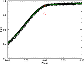
Figure 3. The illustration of data resampling. The black points are the observational data, and the green curve is the fit. The red plus is the interpolated point on the green line, at the same phase the red circle is the averaged flux of all the black points.
Download figure:
Standard image High-resolution imageOf course, we can solve the second disadvantage by shortening the averaging width around the target phase, but it will cause the problem of the few data points. To overcome these two disadvantages, we use curve fitting instead of averaging. Figure 3 demonstrated our method. First, we make a polynomial fit on the black points shown by the green curve. Then, we interpolate the target phase (the phase of the red point) on the fitting curve. The interpolated flux (the flux of the red puls) is the resampled flux. This method can select a wide enough phase to ensure enough data points and so avoid the first disadvantage. With an appropriate fitting degree (for the two targets in this paper, the degree is 20), the light curve section can be fitted very well and so to avoid the second disadvantage.
2.3. Data Points Arrangement
How to arrange the resampled data points is also a problem that needs careful consideration. Figure 4 shows the resampled data points of two different arrangements. The first kind (panel (a)) is that the data points are evenly distributed on phase, see the lower horizontal points which have the same phase values but all the fluxes become 0.25. It can be seen that the phase interval between two neighboring points is uniform.
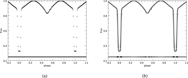
Figure 4. Two kinds of data point arrangements: uniformly distributed on phase (a) and the curve (b). The lower horizontal points are used to show the light curve points distribution on phase.
Download figure:
Standard image High-resolution imageThe second kind of arrangement is different in which the data points will be denser in the phase where the light changes rapidly, see panel (b). Visually, the first kind seems sparse at eclipses, and the second kind seems uniform in all positions. We use the second kind in this paper. For a part of the light curve, we believe that the faster the light changes, the more it can reveal the binary structure and the greater the limitation and influence will be, such as the eclipse parts. In the case of a long-period detached binary star, its transient eclipse almost determines all the results of the light analysis. We believe that the fast-changing parts should have more weight, or should be allocated with more intensive data points. Besides, enough dense data points are needed to exhibit fast light variation. For the two binaries in this paper specifically, how to arrange the points on different parts of the light curve? We adopted an artistic approach. The final effect is that if we fill the light curve, from 0 to 1 in phase, into a square plot area, the data points should be evenly distributed along the curve, that is, the length of the curve between two adjacent points is the same. This arrangement is not only visually beautiful but also effective in the binary light curve analysis.
3. Spectral Data and Observation
LAMOST (Large Sky Area Multi-Object Fiber Spectroscopic Telescope, the new official name is Guoshoujing Telescope) carried out intensive observations on Kepler targets especially. For the two targets here, LAMOST observed KIC 4245897 on June 3rd, 2017 with a high signal to noise ratio, and provided the atmosphere parameters based on the software ULySS (Universite de Lyon Spectroscopic analysis Software; Koleva et al. 2009; Wu et al. 2011a, 2011b, 2014). KIC 2719436 was not observed by LAMOST, and so we carried out spectroscopic observation on 2019 November 13rd using the BFOSC (Beijing Faint Object Spectroscopy and Camera) equipped on the 2.16 m telescope at Xinglong Station, National Astronomical Observatories, Chinese Academy of Sciences. The spectral data were reduced by IRAF (Image Reduction and Analysis Facility) in a standard procedure, including bias subtraction, flat correction, wavelength calibration, and flux normalization. The resulting one-dimensional spectrum was analyzed by SP_ACE spectral analysis tool (Boeche & Grebel 2016) to obtain the atmosphere parameters, and the fit is shown in Figure 5. All the parameters of the two targets are list in Table 1.
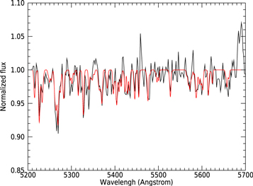
Figure 5. The spectra of KIC 2719436 observed by 2.16 m telescope (black line) and the fit by SP_ACE (red line) at wavelength 5200–5700 Angstrom. The spectra shown here were binned by averaging 6 points to be one point because the original spectra were too chaotic to display clearly.
Download figure:
Standard image High-resolution imageTable 1. The Atmosphere Parameters of KIC 2719436 and KIC 4245897
| Parameters | Value | Value |
|---|---|---|
| KIC name | KIC 2719436 | KIC 4245897 |
| Teff (K) | 6306 ± 330 | 7484 ± 58 |

|
4.16 ± 0.4 | 3.24 ± 0.1 |
| [Fe/H] | −0.94 ± 0.15 | 0.25 ± 0.05 |
Download table as: ASCIITypeset image
4. Binary Light Curve Analysis and the Relative Parameters
Section 2 describe how to obtain the light curves for the binary analysis, and this section will introduce the results of the analysis. The binary light curve analysis program is the Wilson-Devinney code (WD; Wilson & Devinney 1971; Wilson 1979, 1990; van Hamme & Wilson 2007; Wilson 2008; Wilson et al. 2010; Wilson 2012). WD code is sophisticated on physics and numerical convergence, and it was used to derive relative binary parameters for countless times (e.g., Wilson & Devinney 1973; Qian & Yang 2005; Zhang et al. 2017). The binary light analysis results are listed in Table 2, and the light curve fits and the mass-ratio search curve are displayed in Figure 6. The third light L3/(L1+L2+L3) of KIC 2719436 is fixed at zero. Actually, we did carry out the analysis with a third light, but no converged solutions can be obtained. So only the zero third light can fit the light curves.
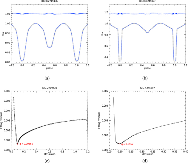
Figure 6. (a) and (b): Phase-binned light curves and the fits, the horizontal distributed points on the upper parts are the fitting residuals. (c) and (d): The mass-ratio search curves to show the mass-ratios of the best fitting.
Download figure:
Standard image High-resolution imageTable 2. The Relative Parameters of KIC 2719436 and KIC 4245897
| Parameters | Value | Value |
|---|---|---|
| KIC Name | KIC 2719436 | KIC 4245897 |
| Period (d) | 0.743479 | 11.257821 |
| Type | semi-detached | semi-detached |
| Inclnation i(°) | 74.78(12) | 86.30(27) |
| M2/M1 | 0.09555(68) | 0.0962(24) |
| T2/T1 | 0.86886(88) | 0.5834(31) |
| R2/R1 | 0.40366(55) | 2.700(19) |
| R1/A | 0.50211(38) | 0.07523(43) |
| R2/A | 0.20268(23) | 0.20309(78) |
| L1/(L1 + L2) | 0.917885(47) | 0.62783(79) |
| L2/(L1 + L2) | 0.082115(47) | 0.37217(79) |
| L3/(L1 + L2 + L3) | 0(fixed) | 0.0692(34) |
| ρ1 (ρ⊙) | 0.17501(29) | 0.2268(26) |
| ρ2 (ρ⊙) | 0.254243(56) | 0.00110920(86) |
Note. M, T, R, A, L, and ρ stand for mass, effective temperature, radius, relative semimajor axis, luminosity in Kepler band, and mean density of the stars, all the parameters are in solar units. The two digits in the parentheses are the errors of the last two digits of the previous number, for example, 0.09555(68) means 0.09555 ± 0.00068.
Download table as: ASCIITypeset image
The exponents g in the gravity brightening law and the bolometric albedos A are fixed at g = 0.32 and A = 0.5 for both components of KIC 2719436 due to their low temperatures and arguably convective envelope, so does the secondary of KIC 4245897. For the primary of KIC 4245897, g = 1 and A = 1 by considering its high temperature. The limb darkening coefficients for the Kepler band are interpolated from the coefficient tables automatically by the program based on the atmosphere parameters. More specifically, the logarithmic limb darkening coefficients are x1 = 0.682, x2 = 0.730, y1 = 0.269 and y2 = 0.212 for KIC 2719436, and x1 = 0.651, x2 = 0.781, y1 = 0.309 and y2 = 0.057 for KIC 4245897.
The binary light curve analysis can provide relative parameters, such as mass-ratio, luminosity-ratio, and radius-ratio. Besides, the light curve can also provide the mean density of the components that can be seen as an absolute physical parameter. The density comes essentially from the period and the relative stellar radius (radius of the stars relative to the semimajor axis  ), see Zhang et al. (2017) for the explanation. The relative size of the stars can be displayed intuitively from the configuration Figure 7. The orbital period is very precise from the photometric observation, so the reliability of the density relies on the relative radius derived from the binary light analysis. The massive practical experience indicates that the relative radius has a very strong correlation to the shape of the light curves. The relative radii of the stars fundamentally determined the eclipse width on the light curves. If the light curve fits are good, the relative radii of the star are reliable. As for the two targets here, the eclipse parts on the light curve can be seen clearly on Figure 6 (inflection points around eclipses, phase ±0.125 for KIC 2719436 and phase ±0.05 for KIC 4245897), so the nice fits make the relative radii in Table 2 are reliable. Therefore the mean densities are reliable consequently.
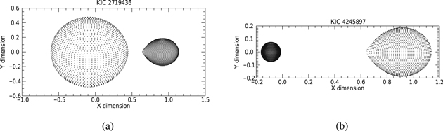
Figure 7. Configuration of the two KIC 2719436 and KIC 4245897 from the light analysis.
Download figure:
Standard image High-resolution imageThe reliability of the densities can be also perceived from the mass-ratio search curves, which have clear bottoms and unambiguously lowest position. A sharp bottom on the mass-ratio search curve increases the reliability of the results (Zhang et al. 2017). For the complete eclipses binaries, such as the two binaries in this paper, the mass-ratio search work can lead to reliable mass ratio and radii, which were applied to calculate the density. Terrell & Wilson (2005) explored the accuracy of photometric mass ratios by comparing to spectroscopic mass ratios and by numerical simulations, and they concluded that complete eclipses lead to reliable mass ratio and radii for over-contact binaries and semi-detached binaries.
5. Absolute Parameters by Two Methods
To obtain the absolute parameters of the binaries, especially the mass and radius, two methods were used. The first method is the commonly used isochrone interpolation but applied to binary stars instead of single stars. In the case of binaries, the atmosphere parameters from spectral data were used to estimate the primary absolute parameters with the help of the isochrone database. The spectra observed are mainly contributed by the light of the primary component stars (defined as the more luminous components), thus the atmosphere parameters derived from the spectra should mainly stand for the primary surface. Therefore, the absolute parameters estimated by the atmosphere parameters should close to that of the primary stars. This assumption was proved statistically by Zhang et al. (2019) to be working within acceptable errors. In the case of LAMOST spectra, this assumption is generally valid. If the physical properties derived by this method have a big divergence from the real values, there might have been two possible reasons. First, the atmosphere parameters were not accurate, such as  often bears large uncertainty. Second, there is a significant third light mixed with the binary light (note: the third light is not necessary from a third body gravitational bound to the binary system, but is also possible from a nearby bright star that is not resolved on observation due to the low spatial resolution), which heavily contaminates the spectra of binary stars. In this case, the observed spectra cannot reflect the primary star.
The second method to estimate the absolute parameters is called the density-temperature method (ϱ–T method; see Zhang et al. 2017 as the example of usage). In short, the difference of this method from the first one is just replacing the  with the density. Because the
  measured from spectra often has big errors, its degree of uncertainty is much greater than that of temperature and metallicity. However, the density, as described in the above section, is arguably reliable when the light curves and fits are good, and it is rarely affected by a third body. For this reason, the ϱ–T method is more reliable than the first method. Practical experience shows that this method is very flexible. Even the metallicity [Fe/H] is unknown (no spectra was observed), a rough temperature can still give low-error absolute parameters. The underlying reason is that density is a very strict restriction on the stars, only density and temperature can limit the possible range of the parameters very well. Figure 8 exhibits how the M1 and R1 are obtained by the ϱ–T method.

Figure 8. The M–R diagram used to derive M1 and R1. The black points are the stars from the isochrone database PARSEC with the same temperature and metallicity as the targets within their errors, T = 6306 ± 330 K and [Fe/H] = −0.94 ± 0.15 for KIC 2719436, and T = 7484 ± 58 K and [Fe/H] = 0.250 ± 0.050 for KIC 4245897. The green lines stand for the mean density of the primary stars, ρ1 = 0.17501 ± 0.00029 ρ⊙ for KIC 2719436 and ρ1 = 0.2268 ± 0.0026 ρ⊙ for KIC 4245897. Actually, there are two green lines in each panel (too close to distinguish by eyes) indicating the error range of the density. The black points between the two green lines are the stars we need to estimate the M1 and R1 of the targets. The red cross stands for the average value of the black points between the two green lines. The errors of M1 and R1 are the mean distance of the red cross to the left and right borders.
Download figure:
Standard image High-resolution image
The isochrone database we used is PARSEC (PAdova and TRieste Stellar Evolution Code, Bressan et al. 2012; Chen et al. 2014, 2015; Tang et al. 2014) version CMD 3.3. The two-part-power law initial mass function (Kroupa 2001, 2002; Kroupa & Weidner 2003) was used, and the coefficient of Reimers mass-loss formula ηReimers = 0.2 on RGB stage.
A problem that needs to be noted is that the isochrone database is based on single stars, the two targets here, however, are binary systems whose primary had already accrete a large amount of mass from their companions and so making their evolution paths far different from single stars. In this case, are the basic parameters interpolated from the isochrone database reliable? The answer is yes. Although all the stars from the database were computed as single stars, every star is self-consistent and balanced. Stars with the same basic parameters (mass, radius, luminosity, etc.) should have the same atmosphere parameters, regardless of their evolutionary history. No matter the current mass of a star, for example, is totally original or partly from accretion, its atmosphere parameters should be the same as those stars with the same basic parameters. Therefore, it is valid to estimate the current basic parameters from the atmosphere parameters, but not valid to indicate its historic evolutionary parameters as single stars.
The next question is: can the secondary absolute parameters be obtained with the above two methods. The answer is no. Because the atmosphere parameters should be attributed to the primary star, the secondary atmosphere parameters are unknown and so do the absolute parameters. Nevertheless, since the relative parameters (e.g., M2/M1 and R2/R1) are already worked out by the binary light curve analysis, the secondary absolute parameters can be calculated consequently. The reliability of the secondary parameters depends on that of the primary parameters and the relative parameters. The accuracy of the isochrone database, of course, will also affect the results, but its impact is insignificant because of the errors of the atmosphere parameters. The absolute parameters are listed in Table 3. According to the comparison of the two methods above, the values from the ϱ–T method are recommended.
Table 3. The Absolute Parameters of KIC 2719436 and KIC 4245897
| Parameters | Value | Error | Value | Error | Methoda |
|---|---|---|---|---|---|
| KIC name | KIC 2719436 | KIC 4245897 | ⋯ | ||
| M1 (M⊙) | 0.83 | 0.24 | 2.7 | 0.51 | TgF |
| M1 (M⊙) | 1.21 | 0.45 | 1.58 | 0.49 | ϱ–T |
| R1 (R⊙) | 1.24 | 0.81 | 6.4 | 2.1 | TgF |
| R1 (R⊙) | 1.89 | 0.25 | 1.9 | 0.28 | ϱ–T |
| M2 (M⊙) | 0.079 | 0.023 | 0.261 | 0.056 | TgF |
| M2 (M⊙) | 0.116 | 0.044 | 0.153 | 0.051 | ϱ–T |
| R2 (R⊙) | 0.5 | 0.33 | 17.3 | 5.8 | TgF |
| R2 (R⊙) | 0.76 | 0.1 | 5.14 | 0.79 | ϱ–T |
| T1 (K) | 6306 | 330 | 7484 | 58 | measured from spectra |
| T2 (K) | 5479 | 292 | 4366 | 57 | from T1 and T2/T1 |
| log(Age) (yr) | 10.01 | 0.97 | 8.74 | 0.22 | TgF |
 (yr) (yr) |
9.62 | 0.54 | 9.09 | 0.64 | ϱ–T |
Note.
aTgF method is the isochrone interpolation based on Temperature, logg, and [Fe/H], and so called TgF. The ϱ–T method is the density-temperature method. The values from ϱ–T method are recommended.Download table as: ASCIITypeset image
The most reliable and generally accepted method to derive the absolute parameters is the double-lined radial velocity observations. By which method the mass-ratio obtained is much more convincing than the light curve analysis. However, for the two binaries here, the double-lined radial velocity observation is quite a challenge in the sense of technology. The double-lined spectral observation requires not only the high-resolution of wavelength and very sensitive instrument but also the moderate difference between the two components. Generally speaking, the mass-ratio is at least greater than 0.5 to measure the double-lines accurately (Yakut & Eggleton 2005), while the mass-ratios of our targets are all below 0.1. Eggleton & Yakut (2017) studied 60 double-lined binaries, and the mass-ratios are mostly close to 1 with a few of them near 0.5 and the minimum is 0.39. The double-lined observation for extreme mass-ratio binaries is arguably very difficult and impractical for a long time, especially for the long period and low mass binaries due to the low radial velocity amplitude.
Since the double-lined observation is hard to achieve, the single-lined observation is much easier and realistic. Although the single radial velocity is helpful to obtain the absolute parameters, the key parameter mass-ratio still depends on the light curve analysis. The single radial velocity cannot provide a substantial contribution to reducing the uncertainty on the final results. Given this, we adopted a more economical way that a single spectrum was observed to measure purely the primary atmosphere parameters.
6. Conclusion and Discussion
From the short-cadence Kepler photometric data, two semi-detached binaries with extremely low mass-ratios and flat-bottom eclipses were found. The bigger components can completely block out the other one, and the flat-bottom eclipse can strongly determine the relative size between the two components. It is generally believed that the light analysis results on total eclipse binary are reliable.
With the help of LAMOST spectra and our spectral observation using the 2.16 m telescope, all the relative and absolute parameters were obtained. Both the two binary systems have excellent light curves and decent spectral data. Two targets all have mass-ratios (slightly) less than 0.1 with the expanded secondary stars.
From the configure Figure 7, we can see the relative size of the two components is different between the two targets. The classical semi-detached binary has a much bigger but less massive secondary star than its primary star like KIC 4245897, which is a well-known phenomenon called the Algol paradox. Interestingly, KIC 2719436 does not conform to the characteristics of the classic Algol by having a much smaller secondary star. This abnormal result can be seen directly from the light curve that KIC 2719436 has a flat-bottom secondary eclipse instead of the usually flat-bottom primary eclipse. The flat-bottom secondary eclipse indicates that the whole secondary star is blocked by the primary star. In other words, the secondary star is smaller than its companion so that it can be fully blocked.
The abnormal configuration of KIC 2719436 does not conflict with resolving the theory of the Algol paradox (Pustylnik 1998), it is the inevitable result of further mass transfer after the Algol stage. The much more further mass transfer will make secondary radius smaller but the primary radius larger, and eventually make the primary star become the bigger one. However, the process of further mass transfer is not easy for most of Algol stars, because the change of the secondary Roche Lobe will impede the mass transfer. When the mass-ratio is lower than 0.78, the mass transfer from secondary to primary will make the secondary Roche Lobe larger, which will lead the secondary star detached from its Roche Lobe and so no more mass transfer. If the mass transfer can persist, the secondary star must expand fast enough to fill its Roche Lobe all the time, or the binary system loses the angular momentum quickly to shrink the distance between the two components as well as the absolute size of the secondary Roche Lobe.
These two binaries are just opposite on the relative size between the two components, and their orbital periods are one short (0.743479 d for KIC 2719436) and long (11.257821 d for KIC 4245897). The reason for the contrary configuration may simply be the initial distance (or period) between the two components at birth.
The initial distance and period of KIC 2719436 are close and short, so does the Roche Lobe of its initial massive star (i.e., the current secondary star). The initial massive star can fill its Roche Lobe at the subgiant stage to start the mass transfer, so its current radius can be small. For KIC 2719436, because the initial distance and period are relatively far and long, and the initial massive star can only fill the Roche Lobe at the red giant stage that is much larger than subgiant. The subgiant is easier to lose its mass and becomes the smaller component than a red giant. Therefore, the current secondary of KIC 2719436 can be smaller than the primary, but the secondary of KIC 4245897 can not.
In simple terms, a more initial distant binary will more likely result in a more current distant binary with larger evolved stars, and vice versa. By the way, the reason for different types of binaries, in the sense of statistics, may simply be the initial distance or period (Zhang et al. 2019).
Expansion by evolution alone can hardly make the mass-ratio decrease to 0.1 like the targets here. The secondary mass is just 0.116 ± 0.044 M⊙ (KIC 2719436) and 0.153 ± 0.051 M⊙ (KIC 4245897), and it is difficult to maintain sufficient internal nuclear reaction with such a small mass. More probably, the angular momentum loss supports the persistence of mass transfer. Two reasons that can decrease the angular momentum. First, the magnetic braking of the stars. Second, the angular momentum extraction from the extra bodies. The first reason requires a strong magnetic field. The KIC 2719436 and KIC 4245897 both have the stars cooler than 7200 K. The envelope of the cool component stars should be convective, which is the basis for the existence of a strong magnetic field. The frequent stellar flares found on the light curves, 145 times for KIC 2719436, and 219 times for KIC 4245897 (Davenport 2016), is direct evidence of a strong magnetic field. Therefore, the magnetic braking is a possible reason that makes the mass-ratio extremely low.
Eggleton & Yakut (2017) suggested that the binaries with an initial mass ratio close to 1 (q = 1–1.4) will turn out to be semi-detached binaries with a longer period, and binaries with mass-ratio above 1.4 will become contact binaries. Accordingly, the initial mass-ratio of KIC 2719436 and KIC 4245897 may be close to 1, and the initial periods may be shorter than the current values. Magnetic braking is the main mechanism to remove angular momentum, and tidal friction was also effective when the orbit was eccentric in the past.
The second reason requires a massive and close extra body. A small mass or distant extra body cannot provide effective angular momentum extraction. No period changes were found based on the high precision times of minima, which indicate a massive and close extra body may not exist. The marginal third light L3/(L1+L2+L3) in Table 2 derived from binary light curve analysis does not support an obvious third body either. Therefore, the angular momentum extraction from an extra body is probably not the reason for the extremely low mass-ratio.
If the mass transfer continues to exist on these two semi-detached binaries, what will be their ends? A natural idea is that the secondary stars will eventually lose all their mass and disappear, so the binaries will become to be single stars. Whether they can become single stars depends on whether the angular momentum loss can persist to the end. The magnetic braking from the primary star will support the last-minute mass transfer. However, the magnetic braking from the secondary stars cannot be effective when their mass approach zero. At this point, KIC 2719436 may end up as a single star, but KIC 4245897 is unlikely because its primary temperature is too high (>7200 K) to have a strong magnetic field.
There is another question about the ends of these two binaries: will they become contact binaries? It still depends on the degree of angular momentum loss. A very effective angular momentum loss will make two components contact each other to be a contact binary. Even so, the contact phase probably will not last forever because the surface temperature difference between the two components is huge. The secondary star will be heated and expanded rapidly right after the contact, and then lost its mass that will enlarge its Roche Lobe and break the contact stage. This is what the TRO (thermal relaxation oscillation) theory predicted. The system will oscillate back and forth between the near-contact and the semi-detached phase, and merges into a single star eventually (Eggleton & Yakut 2017).
The case of KIC 2719436 provides us an upcoming end of a single star for the semi-detached binary, which is possibly the closest target to the end predicted by the theory. However, such an outcome may be rare to find given the abnormal configuration of KIC 2719436.
The photometric data used in this paper were obtained from the Kepler mission and the spectral data were observed by the LAMOST telescope and the 2.16 m telescope at Xinglong Station, National Astronomical Observatories. Guoshoujing Telescope (the Large Sky Area Multi-Object Fiber Spectroscopic Telescope LAMOST) is a National Major Scientific Project built by the Chinese Academy of Sciences. Funding for the project has been provided by the National Development and Reform Commission. LAMOST is operated and managed by the National Astronomical Observatories, Chinese Academy of Sciences. Funding for the Kepler mission is provided by the NASA Science Mission directorate. We acknowledge the support of the staff of the Xinglong 2.16 m telescope. This work was partially supported by the Open Project Program of the Key Laboratory of Optical Astronomy, National Astronomical Observatories, Chinese Academy of Sciences.
This work is supported by the Chinese Natural Science Foundation (grant Nos. 11703082, 11933008 and 11703080) and the Yunnan Natural Science Foundation (grant No. 2018FB006).
Footnotes
- 4
Kepler data processing handbook, http://archive.stsci.edu/kepler/manuals/KSCI-19081-003-KDPH.pdf.