A Comparative Study of Two Fractional-Order Equivalent Electrical Circuits for Modeling the Electrical Impedance of Dental Tissues


Abstract
:
1. Introduction
- Riemann–Liouville and Caputo for continuous-time domain,
- Grünwald–Letnikov in the discrete domain.
2. Materials and Methods
2.1. Human Teeth Dentin Samples Preparation and Data Collection
2.2. The Double Dispersion Cole Bioimpedance Model and Data Reconstruction
2.3. Proposed Recurrent Electrical Impedance Model with Optimal Values
3. Results and Discussion
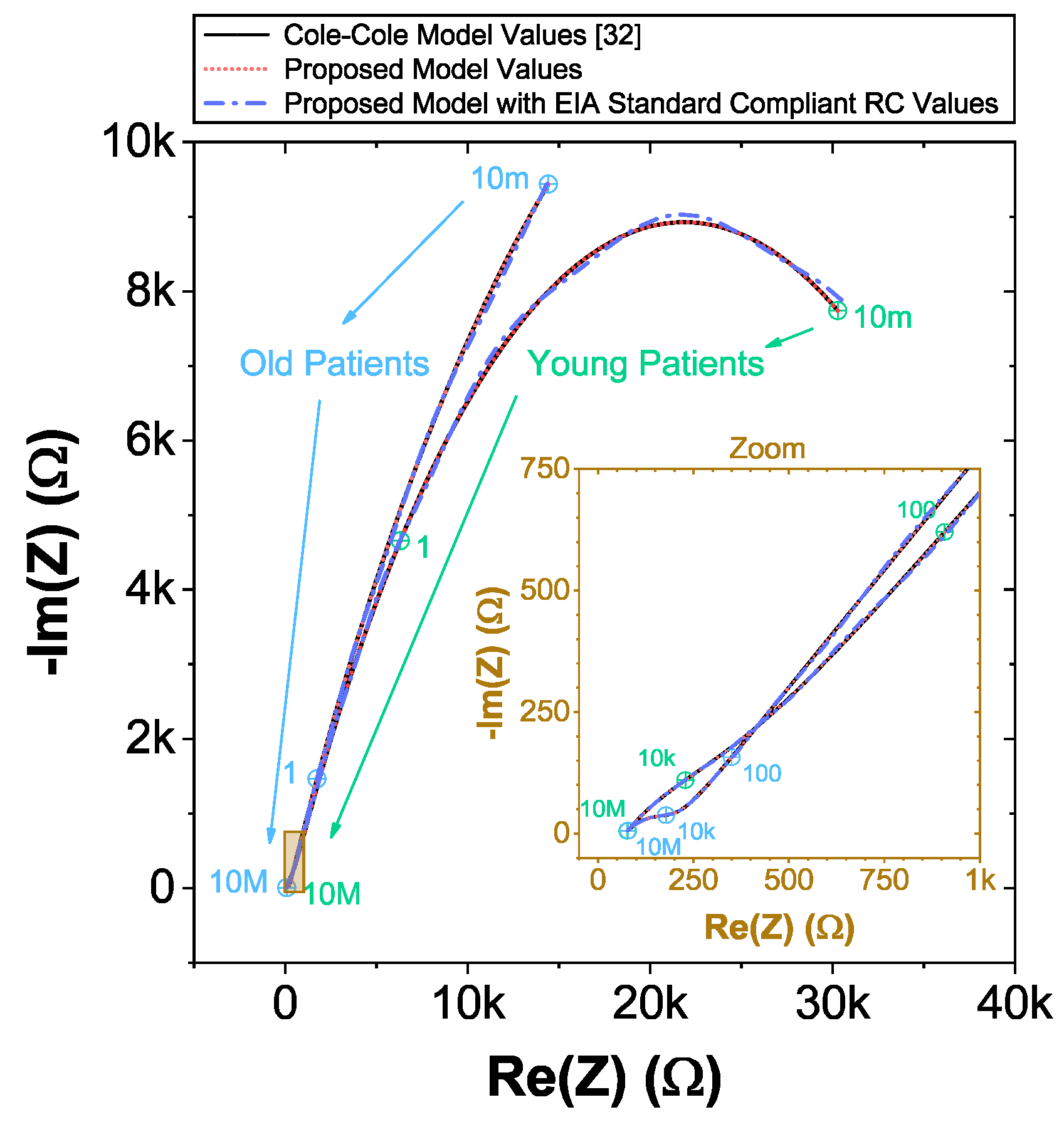
3.1. Comparison of Proposed Bioimpedance Models
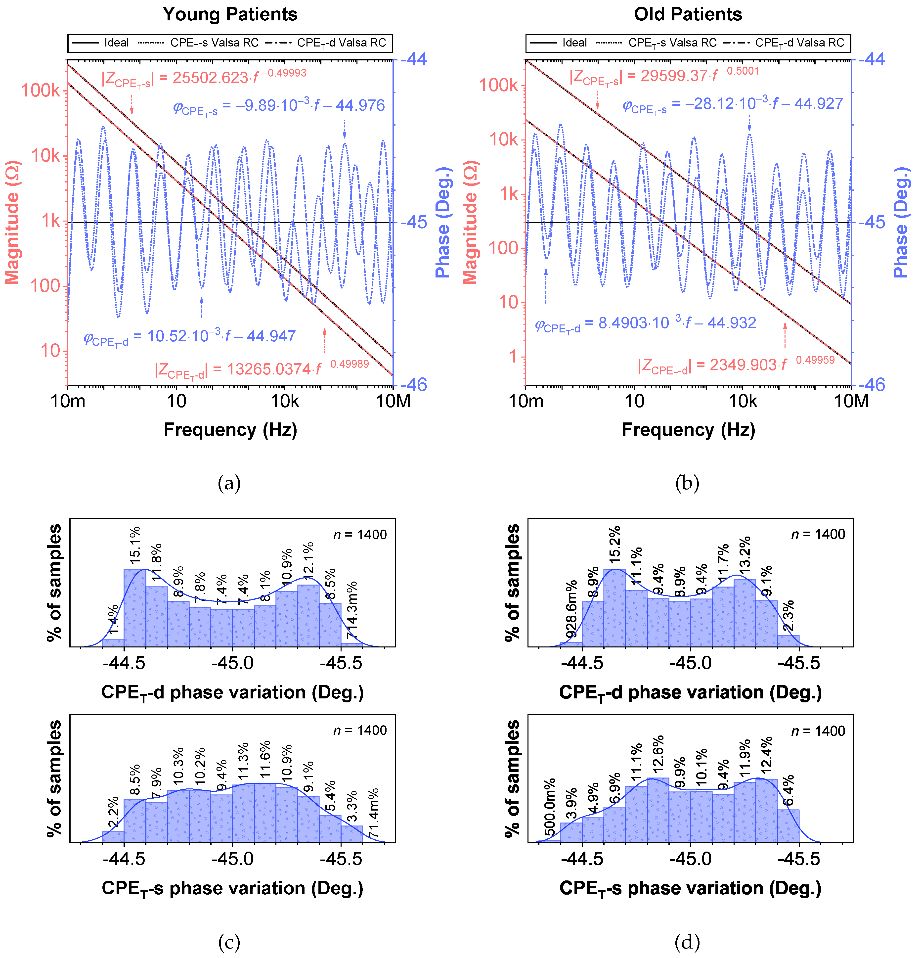
3.2. Empirical Electrical Model of CPEs via Valsa Method
4. Conclusions
Author Contributions
Funding
Acknowledgments
Conflicts of Interest
Abbreviations
| C-C | Double dispersion Cole impedance model |
| CNLS | Complex nonlinear least-squares |
| CoV | Coefficient of variation |
| Order of constant phase element | |
| Pseudo-capacitance of constant phase element | |
| CPE | Constant phase element |
| EIA | Electronic Industries Alliance |
| EIS | Electrical impedance spectroscopy |
| FOC | Fractional-order capacitor |
| FOE | Fractional-order element |
| FOI | Fractional-order inductor |
| LCE | Legates’s coefficient of efficiency |
| MAE | Mean absolute error |
| NSE | Nash–Sutcliffe’s efficiency |
| Coefficient of determination | |
| R, X | Real, imaginary parts of the complex impedance |
| Rec-2 | Recurrent electrical impedance model for bifurcations |
| RMSE | Root mean squared error |
| SD | Standard deviation |
| WIA | Willmott’s index of agreement |
| Mean value |
References
- Ionescu, C.; Lopes, A.; Copot, D.; Machado, J.A.T.; Bates, J.H.T. The role of fractional calculus in modeling biological phenomena: A review. Commun. Nonlinear Sci. Numer. Simul. 2017, 51, 141–159. [Google Scholar] [CrossRef]
- Atangana, A.; Secer, A. A Note on Fractional Order Derivatives and Table of Fractional Derivatives of Some Special Functions. In Abstract and Applied Analysis; Hindawi: London, UK, 2013; pp. 1–8. [Google Scholar] [CrossRef] [Green Version]
- Caponetto, R.; Machado, J.T.; Murgano, E.; Xibilia, M.G. Model Order Reduction: A Comparison between Integer and Non-Integer Order Systems Approaches. Entropy 2019, 21, 876. [Google Scholar] [CrossRef] [Green Version]
- Cabrera-López, J.J.; Velasco-Medina, J. Structured Approach and Impedance Spectroscopy Microsystem for Fractional-Order Electrical Characterization of Vegetable Tissues. IEEE Trans. Instrum. Meas. 2020, 69, 469–478. [Google Scholar] [CrossRef]
- Biswas, K.; Bohannan, G.; Caponetto, R.; Lopes, A.M.; Machado, J.A.T. Fractional-Order Devices; Springer: Berlin/Heidelberger, Germany, 2017. [Google Scholar] [CrossRef]
- Gil’mutdinov, A.K.; Ushakov, P.A.; El-Khazali, R. Fractal Elements and Their Applications; Springer: Berlin/Heidelberger, Germany, 2017. [Google Scholar] [CrossRef]
- Kartci, A.; Herencsar, N.; Machado, J.T.; Brancik, L. History and Progress of Fractional-Order Element Passive Emulators: A Review. Radioengineering 2020, 29, 296–304. [Google Scholar] [CrossRef]
- Freeborn, T.J. A Survey of Fractional-Order Circuit Models for Biology and Biomedicine. IEEE J. Emerg. Sel. Top. Circuits Syst. 2013, 3, 416–424. [Google Scholar] [CrossRef]
- Barsoukov, E.; Macdonald, J.R. Impedance Spectroscopy: Theory, Experiment, and Applications, 3rd ed.; John Wiley and Sons: Chichester, UK, 2018; pp. 1–560. [Google Scholar]
- Simini, F.; Bertemes-Filho, P. (Eds.) Bioimpedance in Biomedical Applications and Research; Springer: Cham, Switzerland, 2018; p. 279. [Google Scholar] [CrossRef]
- Rivas-Marchena, D.; Olmo, A.; Miguel, J.A.; Martínez, M.; Huertas, G.; Yúfera, A. Real-Time Electrical Bioimpedance Characterization of Neointimal Tissue for Stent Applications. Sensors 2017, 17, 1737. [Google Scholar] [CrossRef] [Green Version]
- Grossi, M.; Riccò, B. Electrical impedance spectroscopy (EIS) for biological analysis and food characterization: A review. J. Sens. Sens. Syst. 2017, 6, 303–325. [Google Scholar] [CrossRef] [Green Version]
- Mansor, M.A.; Takeuchi, M.; Nakajima, M.; Hasegawa, Y.; Ahmad, M.R. Electrical Impedance Spectroscopy for Detection of Cells in Suspensions Using Microfluidic Device with Integrated Microneedles. Appl. Sci. 2017, 7, 170. [Google Scholar] [CrossRef]
- Lopes, A.M.; Machado, J.A.T.; Ramalho, E.; Silva, V. Milk Characterization Using Electrical Impedance Spectroscopy and Fractional Models. Food Anal. Methods 2018, 11, 901–912. [Google Scholar] [CrossRef]
- Freeborn, T.J.; Fu, B. Fatigue-Induced Cole Electrical Impedance Model Changes of Biceps Tissue Bioimpedance. Fractal Fract. 2018, 2, 27. [Google Scholar] [CrossRef] [Green Version]
- Freeborn, T.J.; Regard, G.; Fu, B. Localized Bicep Tissue Bioimpedance Alterations Following Eccentric Exercise in Healthy Young Adults. IEEE Access 2020, 8, 23100–23109. [Google Scholar] [CrossRef]
- Ihara, S.; Islam, M.Z.; Kitamura, Y.; Kokawa, M.; Lee, Y.C.; Chen, S. Nondestructive Evaluation of Wet Aged Beef by Novel Electrical Indexes: A Preliminary Study. Foods 2019, 8, 313. [Google Scholar] [CrossRef] [PubMed] [Green Version]
- Basak, R.; Wahid, K.; Dinh, A. Determination of Leaf Nitrogen Concentrations Using Electrical Impedance Spectroscopy in Multiple Crops. Remote Sens. 2020, 12, 566. [Google Scholar] [CrossRef] [Green Version]
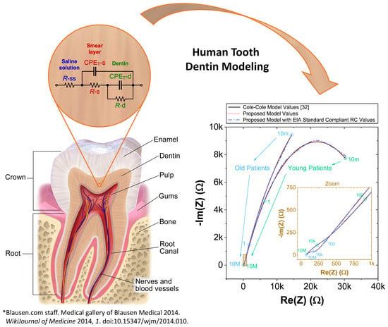
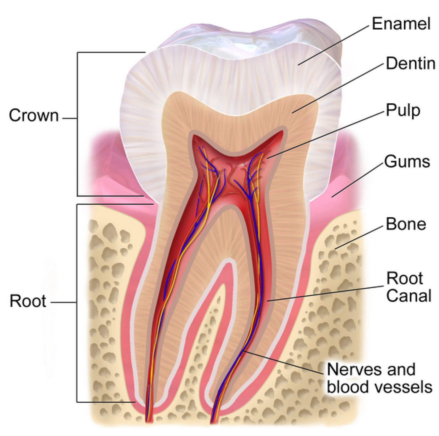
- Blausen.com staff. Medical gallery of Blausen Medical 2014. Wikijournal Med. 2014, 1. [CrossRef] [Green Version]
- Berkovitz, B.K.B.; Holland, G.R.; Moxham, B.J. (Eds.) Oral Anatomy, Histology and Embryology, 5th ed.; Elsevier: Amsterdam, The Netherlands, 2017; p. 472. [Google Scholar]
- Marshall, G.W. Dentin: Microstructure and characterization. Quintessence Int. 1993, 24, 606–617. [Google Scholar]
- Longbottom, C.; Huysmans, M.C.D.N.J.; Pitts, N.B.; Los, P.; Bruce, P.G. Detection of dental decay and its extent using a.c. impedence spectroscopy. Nat. Med. 1996, 2, 235–237. [Google Scholar] [CrossRef]
- Huysmans, M.C.D.N.J.M.; Longbottom, C.; Pitts, N.B.; Los, P.; Bruce, P.G. Impedance Spectroscopy of Teeth with and without Approximal Caries Lesions-an invitro Study. J. Dent. Res. 1996, 75, 1871–1878. [Google Scholar] [CrossRef] [Green Version]
- Longbottom, C.; Huysmans, M.C.D.N.J. Electrical Measurements for Use in Caries Clinical Trials. J. Dent. Res. 2004, 83, C76–C79. [Google Scholar] [CrossRef]
- Pretty, I.A. Caries detection and diagnosis: Novel technologies. J. Dent. 2006, 34, 727–739. [Google Scholar] [CrossRef]
- Morais, A.P.; Pino, A.V.; Souza, M.N. A fractional electrical impedance model in detection of occlusal non-cavitated carious. In Proceedings of the 2010 Annual International Conference of the IEEE Engineering in Medicine and Biology, Buenos Aires, Argentina, 31 August–4 September 2010; pp. 6551–6554. [Google Scholar] [CrossRef]
- Morais, A.P.; Pino, A.V.; Souza, M.N. Detection of questionable occlusal carious lesions using an electrical bioimpedance method with fractional electrical model. Rev. Sci. Instrum. 2016, 87, 084305-1–084305-6. [Google Scholar] [CrossRef]
- Huang, J.H.; Yen, S.C.; Lin, C.P. Impedance Characteristics of Mimic Human Tooth Root Canal and Its Equivalent Circuit Model. J. Electrochem. Soc. 2008, 155, P51–P56. [Google Scholar] [CrossRef]
- Marjanovic, T.; Lackovic, I.; Stare, Z. Comparison of Electrical Equivalent Circuits of Human Tooth used for Measuring the Root Canal Length. Automatika 2011, 52, 39–48. [Google Scholar] [CrossRef]
- Levinkind, M.; Vandernoot, T.J.; Elliott, J.C. Electrochemical Impedance Characterization of Human and Bovine Enamel. J. Dent. Res. 1990, 69, 1806–1811. [Google Scholar] [CrossRef] [PubMed]
- Levinkind, M.; Vandernoot, T.J.; Elliott, J.C. Evaluation of Smear Layers on Serial Sections of Human Dentin by Means of Electrochemical Impedance Measurements. J. Dent. Res. 1992, 71, 426–433. [Google Scholar] [CrossRef] [PubMed]
- Eldarrat, A.H.; Wood, D.J.; Kale, G.M.; High, A.S. Age-related changes in ac-impedance spectroscopy studies of normal human dentine. J. Mater. Sci. Mater. Med. 2007, 18, 1203–1210. [Google Scholar] [CrossRef] [PubMed]
- Kartci, A.; Agambayev, A.; Herencsar, N.; Salama, K.N. Series-, Parallel-, and Inter-Connection of Solid-State Arbitrary Fractional-Order Capacitors: Theoretical Study and Experimental Verification. IEEE Access 2018, 6, 10933–10943. [Google Scholar] [CrossRef]
- Bondarenko, A.S.; Ragoisha, G.A. Inverse problem in potentiodynamic electrochemical impedance spectroscopy. In Progress in Chemometrics Research; Pomerantsev, A.L., Ed.; Nova Science Publishers: New York, NY, USA, 2005; pp. 89–102. [Google Scholar]
- Gueymard, C.A. A review of validation methodologies and statistical performance indicators for modeled solar radiation data: Towards a better bankability of solar projects. Renew. Sustain. Energy Rev. 2014, 39, 1024–1034. [Google Scholar] [CrossRef]
- Valsa, J.; Vlach, J. RC models of a constant phase element. Int. J. Circuit Theory Appl. 2013, 41, 59–67. [Google Scholar] [CrossRef]
- Kartci, A.; Agambayev, A.; Farhat, M.; Herencsar, N.; Brancik, L.; Bagci, H.; Salama, K.N. Synthesis and Optimization of Fractional-Order Elements Using a Genetic Algorithm. IEEE Access 2019, 7, 80233–80246. [Google Scholar] [CrossRef]


| Tissue | Ref. | Year | Frequency Range (Hz) | Preparation of Samples | Model | |
|---|---|---|---|---|---|---|
| # of Elements | Brief Description | |||||
| Root Canal | [28] | 2008 | 10–30 k | One tooth without specified eruption status and patient age. | 6 | Complex model employing three CPEs andthree resistors. |
| [29] | 2011 | 100–1 M | Single incisor tooth without specified eruption status and patient age. | 3 | Single CPE in parallel with series connection of CPE and resistor. | |
| Enamel | [30] | 1990 | 1–65 k | Extracted one tooth from five patients of different age groups (7 to 50 years old) with different eruption status. | 5 | Complex model employing single CPE, two capacitors, and two resistors. |
| Dentin | [31] | 1992 | 1–65 k | Two un-erupted third molars (18 and 38) from one patient. | 4 | Single CPE in parallel with three resistors in series. |
| [32] | 2007 | 10 m–10 M | Five un-erupted third molars from 20 (±1) and 50 (±1) years old patients. | 5 | Double dispersion Cole impedance model. | |
| Components | Elements | Cole-Cole Model Mean Values [32] | Recurrent Model Values | Recurrent Model with EIA Standard Compliant RC Values | |||
|---|---|---|---|---|---|---|---|
| Patients | |||||||
| Young | Old | Young | Old | Young | Old | ||
| Saline solution | R-ss () | 71.5 | 72.1 | 71.5 | 72.1 | 71.5 | 72.3 |
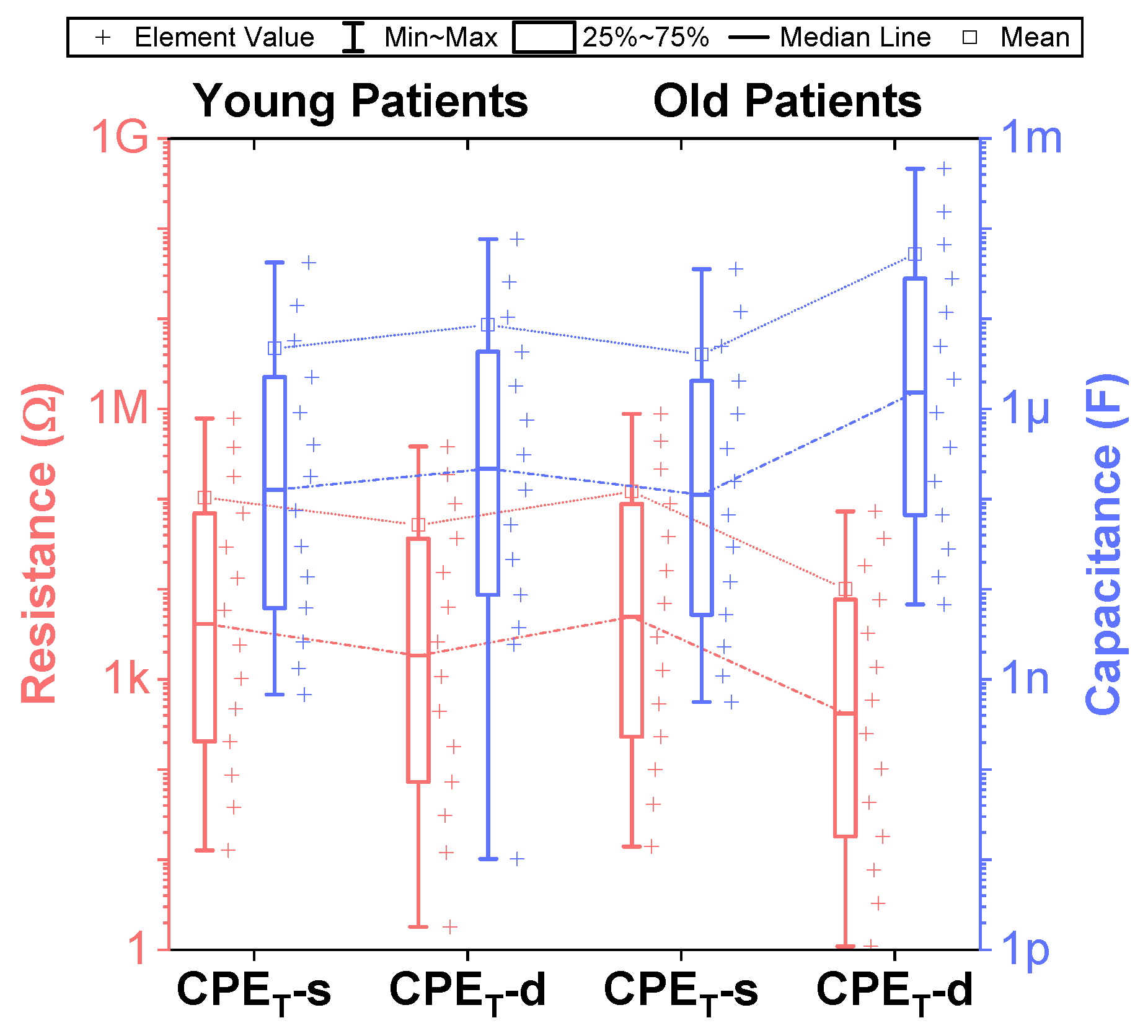
| Smear layer | CPET-s () | 23.8 | 14.6 | 15.64 | 13.52 | 15.6 | 13.5 |
| CPEP-s (−) | 0.5 | ||||||
| R-s () | 244 | 128.1 | 564.3 | 149.38 | 562 | 150 | |
| Dentins | CPET-d () | 45.6 | 182.8 | 30.23 | 169.34 | 30.1 | 169 |
| CPEP-d (−) | 0.5 | ||||||
| R-d (k) | 43.1 | 60.9 | 42.78 | 60.88 | 43 | 60.4 | |
| Evaluation Criteria | Recurrent Model Values | Recurrent Model with EIA Standard Compliant RC Values | ||
|---|---|---|---|---|
| Patients | ||||
| Young | Old | Young | Old | |
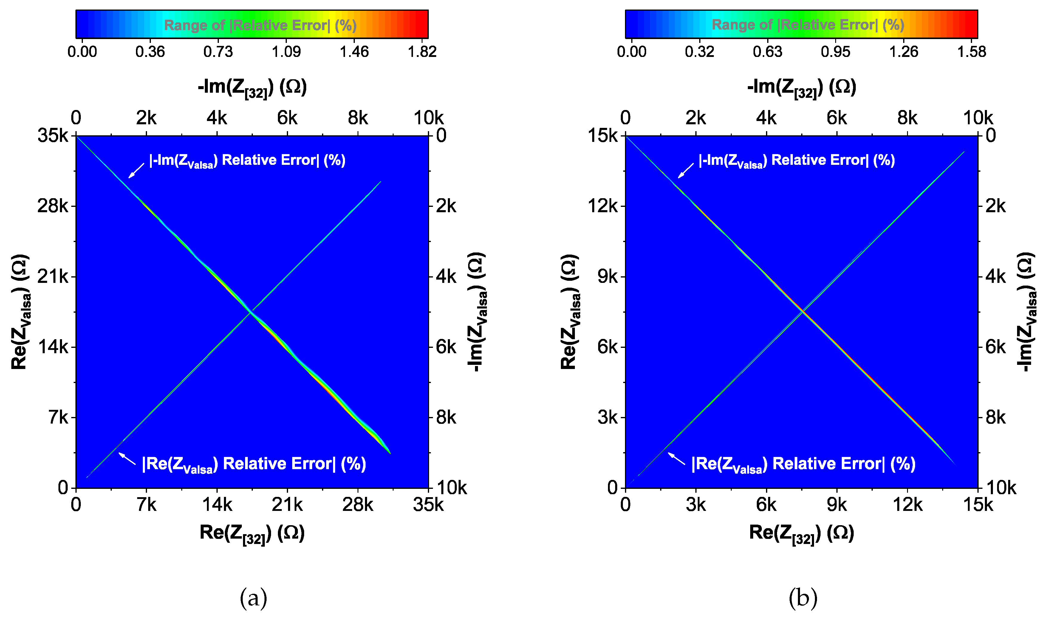
| ∣Re(Z) Relative Error∣ (%) | ||||
| Max | 0 | 0 | 1.047 | 0.905 |
| Mean | 0.330 | 0.345 | ||
| Median | 0.275 | 0.310 | ||
| SD | 0.267 | 0.208 | ||
| ∣−Im(Z) Relative Error∣ (%) | ||||
| Max | 0 | 0 | 1.822 | 1.578 |
| Mean | 0.622 | 0.612 | ||
| Median | 0.579 | 0.588 | ||
| SD | 0.395 | 0.400 | ||
| Evaluation Criteria | Recurrent Model Values | Recurrent Model with EIA Standard Compliant RC Values | ||
|---|---|---|---|---|
| Patients | ||||
| Young | Old | Young | Old | |
| () | 0 | 0 | 19.261 | 6.905 |
| () | 15.734 | 8.730 | ||
| () | 0 | 0 | 41.744 | 16.591 |
| () | 31.781 | 23.817 | ||
| (−) | 1 | 1 | 0.99999 | 0.99998 |
| (−) | 0.99991 | 0.99996 | ||
| (−) | 1 | 1 | 0.99997 | 0.99997 |
| (−) | 0.99989 | 0.99988 | ||
| (−) | 1 | 1 | 0.99999 | 0.99999 |
| (−) | 0.99997 | 0.99997 | ||
| (−) | 1 | 1 | 0.99659 | 0.99650 |
| (−) | 0.99394 | 0.99433 | ||
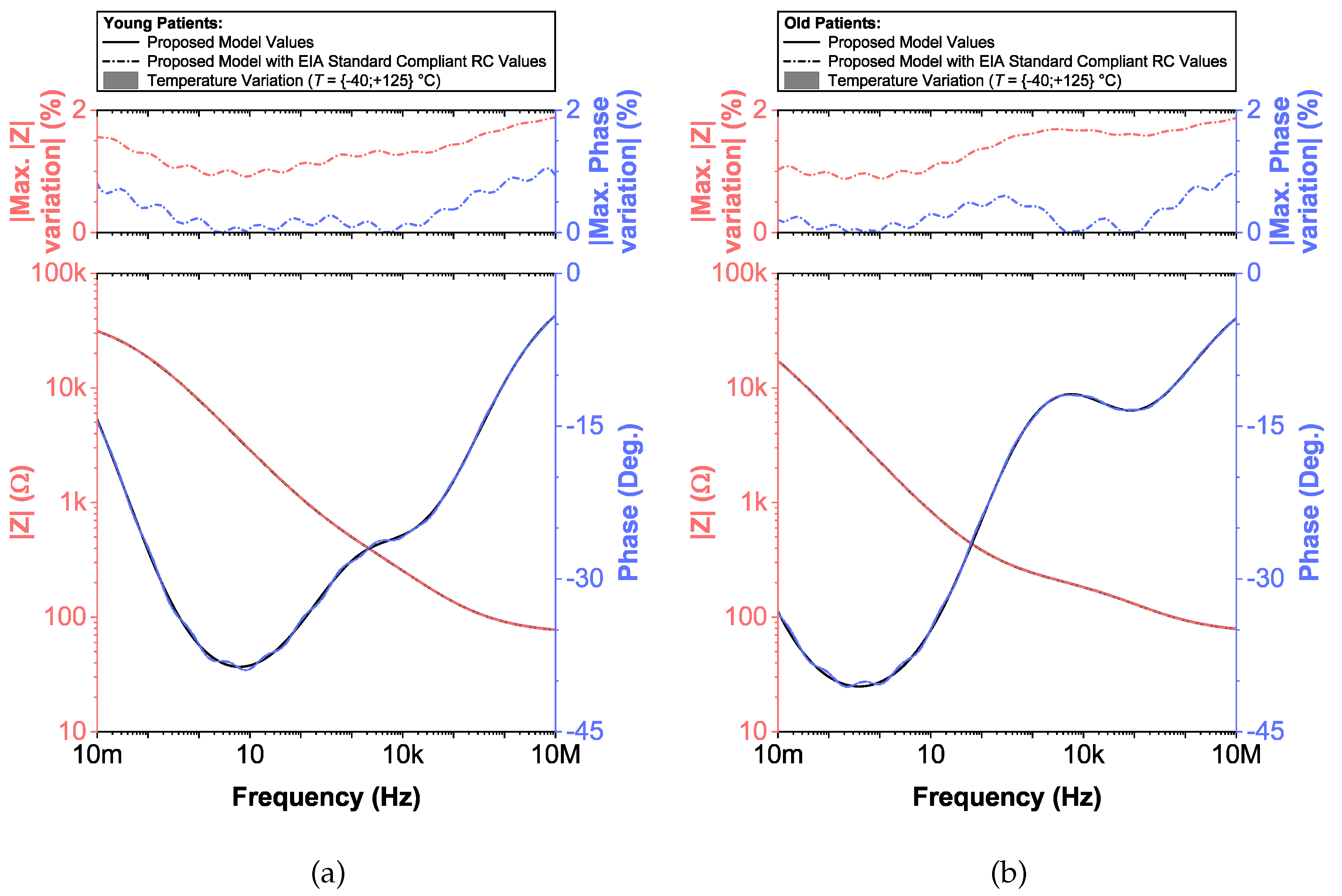
| Elements |  RC Network with Valsa Determined Parameters | |||
|---|---|---|---|---|
| Young Patients | Old Patients | |||
| CPET-s | CPET-d | CPET-s | CPET-d | |
| C0 (F)/R0 () | 680 p/787 k | 10.2 p/383 k | 562 p/887 k | 6.8 n/73.2 k |
| C1 (F)/R1 () | 2.61 n/38.3 | 1.8 /6.34 k | 12.1 n/232 | 66.5 n/7.68 |
| C2 (F)/R2 () | 6.2 n/86.6 | 3.74 n/12 | 29.4 n/536 | 11.8 /1.37 k |
| C3 (F)/R3 () | 30 n/470 | 2.43 n/1.8 | 66.5 n/1.27 k | 4.99 /590 |
| C4 (F)/R4 () | 13.7 n/205 | 8.66 n/30.9 | 158 n/2.94 k | 28 n/3.3 |
| C5 (F)/R5 () | 909 n/13.3 k | 21.5 n/73.2 | 365 n/6.98 k | 13.7 n/1.1 |
| C6 (F)/R6 () | 42.2 /374 k | 4.32 /15.4 k | 35.7 /442 k | 66.5 /7.68 k |
| C7 (F)/R7 () | 1.33 n/12.7 | 52.3 n/180 | 5.23 n/100 | 374 n/43.2 |
| C8 (F)/R8 () | 178 n/2.4 k | 309 n/1.07 k | 887 n/16 k | 909 n/102 |
| C9 (F)/R9 () | 14 /178 k | 76.8 /187 k | 2.32 n/41.2 | 28 /3.24 k |
| C10 (F)/R10 () | 2.26 /29.4 k | 25.5 /88.7 k | 2.05 /38.3 k | 158 n/18.2 |
| C11 (F)/R11 () | 75 n/1.02 k | 127 n/442 | 1.1 n/14 | 2.15 /249 |
| C12 (F)/R12 () | 402 n/5.9 k | 10.5 /36.5 k | 12 /215 k | 464 /36.5 k |
| C13 (F)/R13 () | 5.76 /69.8 k | 750 n/2.61 k | 4.99 /88.7 k | 154 /18.2 k |
| CPEP Values (−)/Phase Angle (Deg.) | ||||
| Mean | 0.500/−45.001 | 0.500/−44.973 | 0.500/−44.997 | 0.499/−44.954 |
| SD | 0.003/0.290 | 0.003/0.315 | 0.003/0.284 | 0.003/0.268 |
| ∣CoV∣ (%) | 0.644 | 0.700 | 0.631 | 0.597 |
| CPET Values () | ||||
| Mean | 15.615 | 30.087 | 13.430 | 169.856 |
| SD | 0.456 | 1.054 | 0.396 | 4.982 |
| ∣CoV∣ (%) | 2.921 | 3.503 | 2.946 | 2.933 |
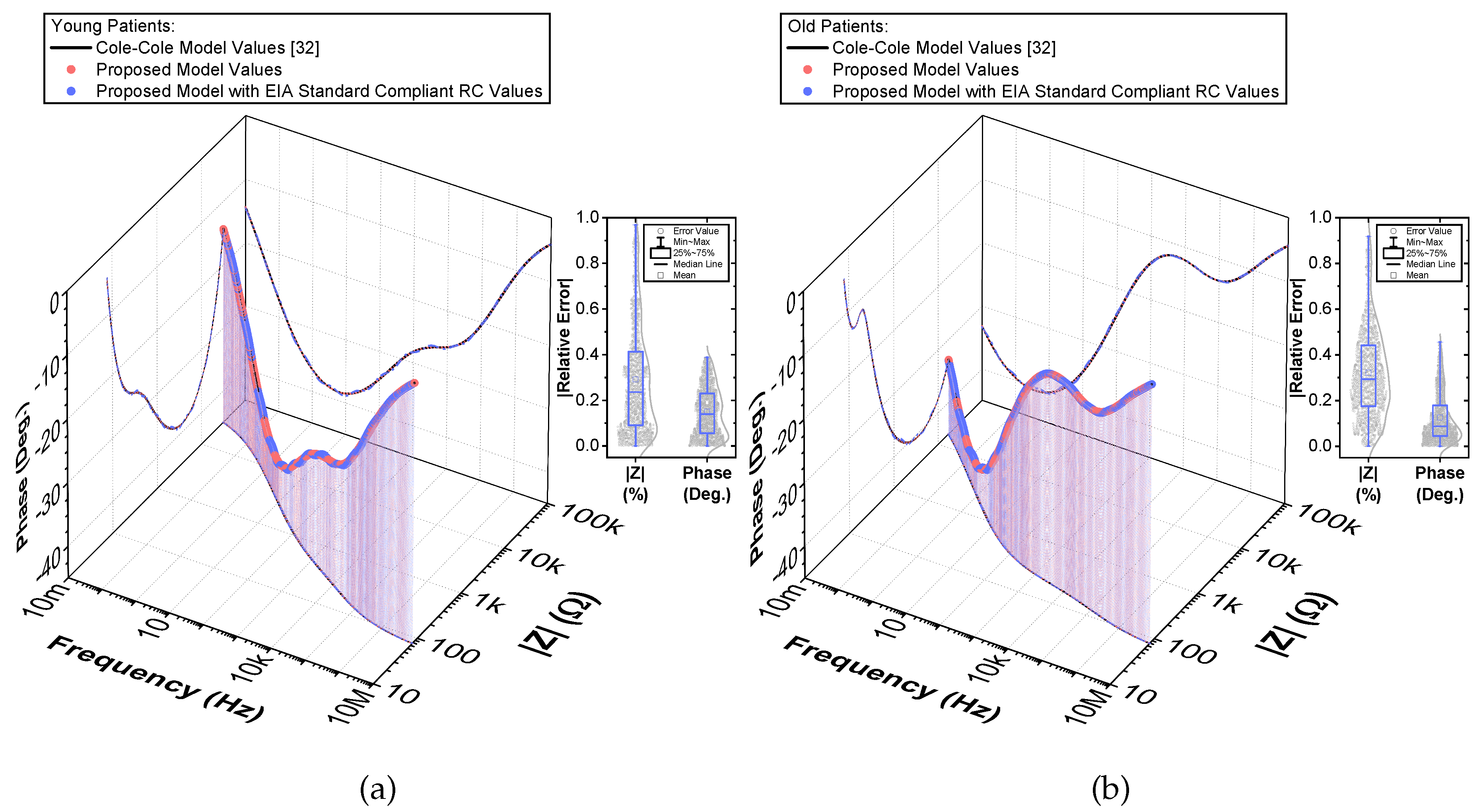
| ∣Relative Magnitude Error∣ (%) | ||||
| Max | 1.150 | 1.188 | 1.075 | 1.188 |
| Mean | 0.467 | 0.493 | 0.420 | 0.481 |
| Median | 0.424 | 0.474 | 0.384 | 0.459 |
| SD | 0.305 | 0.291 | 0.265 | 0.311 |
| ∣Phase Angle Error∣ (Deg.) | ||||
| Max | 0.623 | 0.556 | 0.606 | 0.526 |
| Mean | 0.247 | 0.282 | 0.244 | 0.240 |
| Median | 0.235 | 0.298 | 0.238 | 0.244 |
| SD | 0.153 | 0.143 | 0.145 | 0.129 |
© 2020 by the authors. Licensee MDPI, Basel, Switzerland. This article is an open access article distributed under the terms and conditions of the Creative Commons Attribution (CC BY) license (http://creativecommons.org/licenses/by/4.0/).
Share and Cite
Herencsar, N.; Freeborn, T.J.; Kartci, A.; Cicekoglu, O. A Comparative Study of Two Fractional-Order Equivalent Electrical Circuits for Modeling the Electrical Impedance of Dental Tissues. Entropy 2020, 22, 1117. https://doi.org/10.3390/e22101117
Herencsar N, Freeborn TJ, Kartci A, Cicekoglu O. A Comparative Study of Two Fractional-Order Equivalent Electrical Circuits for Modeling the Electrical Impedance of Dental Tissues. Entropy. 2020; 22(10):1117. https://doi.org/10.3390/e22101117
Chicago/Turabian StyleHerencsar, Norbert, Todd J. Freeborn, Aslihan Kartci, and Oguzhan Cicekoglu. 2020. "A Comparative Study of Two Fractional-Order Equivalent Electrical Circuits for Modeling the Electrical Impedance of Dental Tissues" Entropy 22, no. 10: 1117. https://doi.org/10.3390/e22101117