Dual Path Attention Net for Remote Sensing Semantic Image Segmentation

Abstract

Semantic segmentation plays an important role in being able to understand the content of remote sensing images. In recent years, deep learning methods based on Fully Convolutional Networks (FCNs) have proved to be effective for the sematic segmentation of remote sensing images. However, the rich information and complex content makes the training of networks for segmentation challenging, and the datasets are necessarily constrained. In this paper, we propose a Convolutional Neural Network (CNN) model called Dual Path Attention Network (DPA-Net) that has a simple modular structure and can be added to any segmentation model to enhance its ability to learn features. Two types of attention module are appended to the segmentation model, one focusing on spatial information the other focusing upon the channel. Then, the outputs of these two attention modules are fused to further improve the network’s ability to extract features, thus contributing to more precise segmentation results. Finally, data pre-processing and augmentation strategies are used to compensate for the small number of datasets and uneven distribution. The proposed network was tested on the Gaofen Image Dataset (GID). The results show that the network outperformed U-Net, PSP-Net, and DeepLab V3+ in terms of the mean IoU by 0.84%, 2.54%, and 1.32%, respectively.

1. Introduction

Semantic segmentation is a fundamental aspect of computer vision research. Its goal is to assign a category label to each pixel in an image. Together with other kinds of deep learning research, it plays an important role in the recognition of different types of land cover in remote sensing images [1,2,3]. Recognizing the information an image contains is a key part of remote sensing image interpretation. Semantic segmentation is widely used in land cover mapping and monitoring, urban classification analysis, tree species identification in forest management, etc. [4,5,6,7,8,9,10,11,12]. To accomplish it, land cover types need to be distinguished in terms of “same object, different spectrum”, or “same spectrum, different object”. For instance, “lake” and “river” are two different types of land cover, but in remote sensing, they can have a similar appearance. Places with a high density of buildings or a low density of buildings may still both be classified as urban residential areas. In addition, the boundaries between different types of land cover are intricate and irregular, which makes the remote sensing segmentation task even more difficult. Thus, discrimination between features at a pixel level is essential.

In recent years, the state-of-the-art in semantic segmentation networks has progressed enormously [13,14,15]. One way to solve the above issues is by using a recurrent neural network to capture long-range contextual information. This kind of network can achieve remarkable results. For instance, a directed acyclic graph recurrent neural network [16] can capture the rich contextual information present in local features. However, although this method is very effective, it is largely dependent on longer-term learning results. Obtaining such a large number of remote sensing image segmentation labels is very difficult, so it is of limited practical utility for the segmentation of remote sensing images.

Another effective way of tackling the issues described above is to use self-attention mechanisms. These are popular and simple to adapt to semantic segmentation tasks because of their varied and flexible structure [17,18,19,20,21,22]. Self-attention mechanisms focus on local features by generating weight feature maps and fusing downstream feature maps. This may involve having one or more modules built upon a basic backbone, with each module focusing on things such as the channel or spatial information. However, downstream feature maps can lose a lot of spatial information, and the capture of the original spatial information directly is currently not feasible. Yet, having very precise spatial information is crucial for the effective segmentation of remote sensing images.

To address the above issues, we propose here a novel self-attention mechanism model, called a Dual Path Attention Network (DPA-Net), which is designed for remote sensing semantic segmentation. It uses two attention modules: a total spatial attention module to capture spatial information and a channel attention module to capture the channel information separately. The two modules can easily be appended to other segmentation models such as PSP-Net [23]. At present, there are many methods for the efficient extraction of different kinds of feature information. However, the input of almost all spatial attention methods is the feature map after sampling. As mentioned above, compared with the original image, the downsampled feature map contains a lot less spatial information. Therefore, this kind of spatial attention is inevitably inefficient, as it is unable to fully utilize the spatial information in the data. Therefore, instead of the downsampled image, we changed the input of the spatial attention method to the original image. In the total spatial attention module, spatial information is captured from the original image according to the self-attention mechanism mentioned above. The output of the TSAM is a single channel weight matrix. Each pixel of the output can be updated again by fusing according to the corresponding weight, with the weight itself being generated by the module. After being fused with the final feature map of DPA-Net, the TSAM will provide a weight for each pixel. During the training, the network pays higher attention to the areas with larger weights. This means that each pixel has its own focus in the network. For the channel attention module, the self-attention mechanism captures the channel information according to the channel maps. As with the total spatial attention module, it generates a weight factor. The feature maps are updated by integrating this weight factor. Once the two modules have completed their operations, two feature maps are obtained that contain spatial information and channel information, respectively. Then, these two feature maps are aggregated to generate the final output.

It is worth emphasizing that although the proposed method is more effective than the original self-attention method, it does not significantly change the memory footprint. Overall, it solves the conventional problems associated with self-attention mechanisms in a straightforward way. First of all, the TSAM makes its calculations on the basis of the original image. When compared to downstream feature maps, original remote sensing images contain more spatial information. Secondly, the output of the two modules acts on the last feature map in the model. Thus, the two modules can control the back propagation of the entire model. In addition, the simplicity of the module structure makes it easy for it to be used with any segmentation model. To verify the effectiveness of our method, we conducted experiments with U-Net, PSP-Net, and DeepLab V3+ [24,25] on the Gaofen Image Dataset (GID) [26]. It improved the mean IoU for each module by 0.84%, 2.54% and 1.32%, respectively.

The main contributions of the paper can be summarized as follows:

• We propose a Dual Path Attention Network (DPA-Net) that uses a self-attention mechanism to enhance a network’s ability to capture key local features in the semantic segmentation of remote sensing images.
• A total spatial attention module is used to extract pixel-level spatial information, and a channel attention module is proposed to focus on different features. After the dual path feature extraction has taken place, the performance of the sematic segmentation is significantly improved.
• As the number of images in the test dataset, GID, was rather small, processing strategies were developed to improve the quality of our tests. By extension, these strategies can be used more generally to improve the segmentation of small datasets.

2. Related Work

Remote Sensing. High-resolution remote sensing images form the basic data for spatial information technology in geographic information systems. They are also an important national and international strategic information resource [1,26,27,28,29,30]. The images collected by remote sensors installed on aircraft or satellites underpin remote recognition techniques that aim to recognize land cover, such as buildings, farmland, vegetation, bare soil, rivers, etc. After the land cover has been recognized, thematic maps are often produced to visually represent its distribution. When combined with computer vision algorithms, remote recognition techniques have significant advantages regarding real-time capture and cost when compared to traditional field surveys. Therefore, they are increasingly used in the fields of land-use planning, forestry, and soil-loss monitoring [31,32,33,34].

Semantic Segmentation. Semantic segmentation aims to segment and parse a scene image into different regions associated with semantic categories. In recent years, various methods based on FCNs [35] have led to important breakthroughs in semantic segmentation. One way to improve the performance of a segmentation model is to enhance its contextual aggregation. Several models such as U-Net use an encoder–decoder structure [24,36,37] to integrate midstream features and downstream features. The encoder module gradually reduces the size of the feature maps and captures higher-level semantic information. The spatial information is recovered by the decoder module. Models such as DeepLab V3+ apply atrous spatial pyramid pooling to fuse features at several different scales and across various different sub-regions [25,38,39,40]. Outside of this, parallel dilated convolutions with different dilation rates can enlarge the receptive field. Another effective approach is to capture rich context dependencies. For instance, Peng [41] developed the concept of large kernel matters for learning contextual dependencies using a global convolutional network (GCN). Mnih et al. [42] added an attention mechanism to a recurrent neural network (RNN) to reduce its complexity. Wang et al. [43] were the first to propose a recurrent attention structure for remote sensing images. Here, a mask matrix is used for the attention weights, which then multiply the feature map to obtain an attention-based representation of high-level features.

Self-Attention Mechanisms. Self-attention mechanisms provide an effective way of enhancing the ability of a neural network to capture critical local features. The approach [44] was first proposed for machine translation, but it is now widely used in image classification [1], image segmentation [22], and other fields [45,46,47]. Many studies have shown that attention mechanisms can enhance the identification of neurons with key characteristics and improve a network’s performance. For example, Convolution Block Attention Modules (CBAM) [19] draw on top-level information to get weights channel-wise or spatial activations by concatenating channel and spatial attention modules. In a different approach, DA-Net [22] runs a channel attention module and spatial attention module in parallel in a non-local autocorrelation matrix, which has delivered good results.

3. Methods

In this section, we first present the overall framework of our network; then, we introduce the two attention modules, which capture spatial and channel-related contextual information. The section concludes with a description of how the output from the two modules is aggregated to give the final output.

3.1. Overview

For regular semantic segmentation, the scene for segmentation will include a variety of objects of diverse scales with different lighting that are visible from different viewpoints. However, because of the same shooting angle and distance of the samples in different remote sensing images, the boundary problem can be considered as more than just a multi-scale and multi-angle problem. In a remote sensing image, there will be many different types of land cover. In general, different types of land cover have their own spectral and structural characteristics, which are visible in different brightness values, pixel values, or spatial changes in remote sensing images. On account of the complexity of the composition, nature, distribution, and imaging conditions of the surface features, remote sensing images can be thought of in terms of “same object, different spectrum” and “same spectrum, different object”. There are also two or more kinds of “mixed pixels” that can occur in a single pixel or the instantaneous field of view, making the work of recognition in remote sensing images even more complex. All of these factors can affect the accuracy of the result. To deal with this, our proposed method seeks to enhance the aggregated channel and spatial features separately, thus improving the feature representation for remote sensing segmentation.

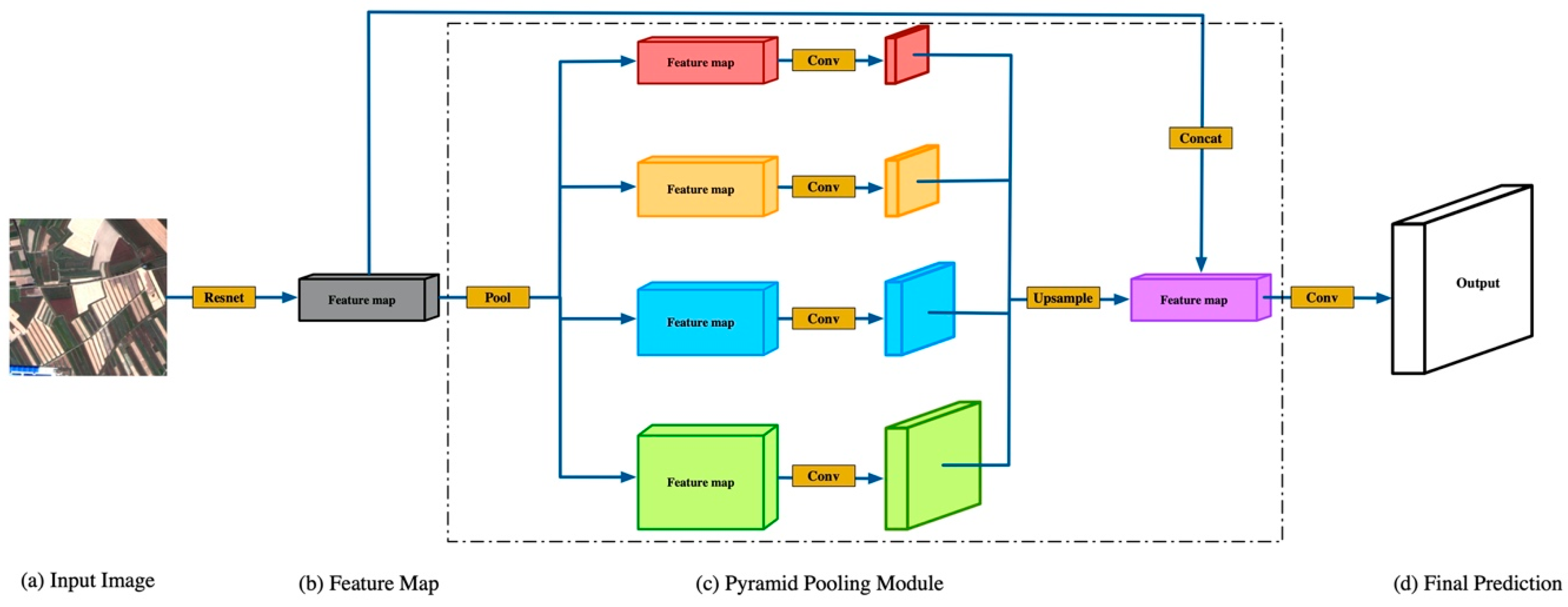
Our method can be used with any semantic segmentation model, such as U-Net, PSP-Net, etc. Taking PSP-Net as an example, its basic structure is shown in Figure 1 [22]. The input image (a) is fed into a Convolutional Neural Network (CNN) to obtain the feature map of the last convolutional layer (b). Then, a pyramid parsing module (c) is used to get different sub-region representations, followed by upsampling and concatenation layers to form the final feature representation. This contains both local and global context information. Finally, a convolutional layer is used to get the per-pixel prediction (d) according to the required representation.

The general structure of DPA-PSP-Net is shown in Figure 2. We employed a pretrained ResNet50 [48] and used a dilated strategy [38] for the backbone. Drawing upon the structure of ResNet50, the proposed framework has four residual blocks, a Pyramid Pooling Module (PPM), a channel attention module, and a spatial attention module. We removed the down-sampling operation and employed dilated convolutions in the last two residual blocks instead, which is identical to the process used in PSP-Net. Thus, the size of the final feature map was at 1/8 of the scale of the input image. Given an input image with a size of 256 px × 256 px, we used ResNet50 to get the feature map, F₁, while the weighting factor for the spatial attention, Ws, was obtained by the spatial attention module. F₁ was fed into the PPM and the channel attention module, respectively, to obtain the feature map, F₂, after up-sampling and applying the weighting factor for channel attention, W_c. Finally, F₂ was multiplied by W_c and W_s to obtain the features to obtain the channel attention-weighted feature map, F_C, and spatial attention-weighted feature map, F_S. Then, F_C and F_S were aggregated to get the final output.

3.2. Total Spatial Attention Module

The effectiveness of the feature extraction is directly related to the accuracy of the results in remote sensing image segmentation. Features can be obtained by using contextual information. However, many studies [23,41] have shown that local features generated by traditional FCNs can lead to the wrong classification of objects and inaccurate prediction of object shapes. The attention mechanism plays an important role in the human visual system. When confronted with complex scenes, human beings can quickly focus their attention on significant aspects and prioritize them. As with the human visual system, a computer-based attention mechanism can focus the computing power of a network on key features, so that important features can be extracted from remote sensing images more effectively and redundant information can be set aside. To enhance the local feature extraction ability for difficult remote sensing images, we have developed a total spatial attention module (TSAM). This module can capture the spatial boundary information of remote sensing images, which makes it easier to extract the boundary features and refine other adaptive features, while suppressing less important information. The structure of the module is very simple, and it can be embedded in any network to improve a network’s feature learning ability. Numerous methods for handling spatial attention already exist [20,22]. However, in our spatial attention module, the input is data rather than a feature map, F₁. In view of the high-resolution character of remote sensing images and the complex spatial information they contain, the accuracy of the boundary information is of vital importance. As a network deepens, the receptive field gradually expands, the semantic information becomes increasingly advanced, the feature map becomes smaller and smaller, and the spatial information is constantly reduced. The size of the feature map, F₁, is only 1/8 of the input data, so a lot of spatial information has been lost. Therefore, the original image is a better resource for capturing the important spatial information in a remote sensing image.

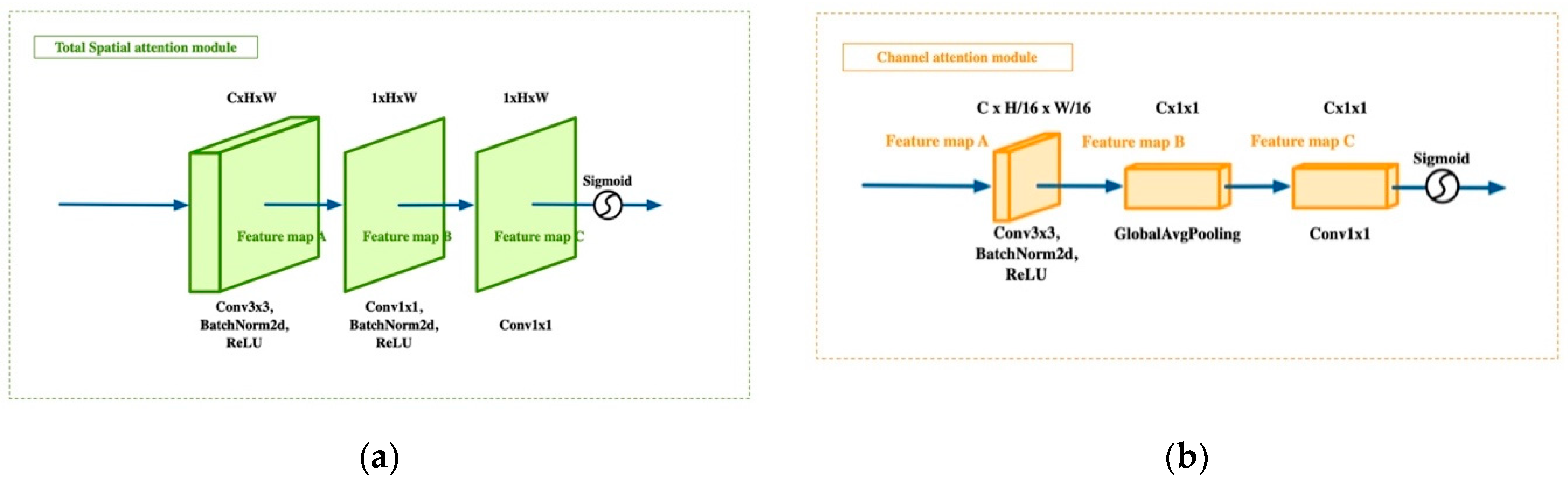
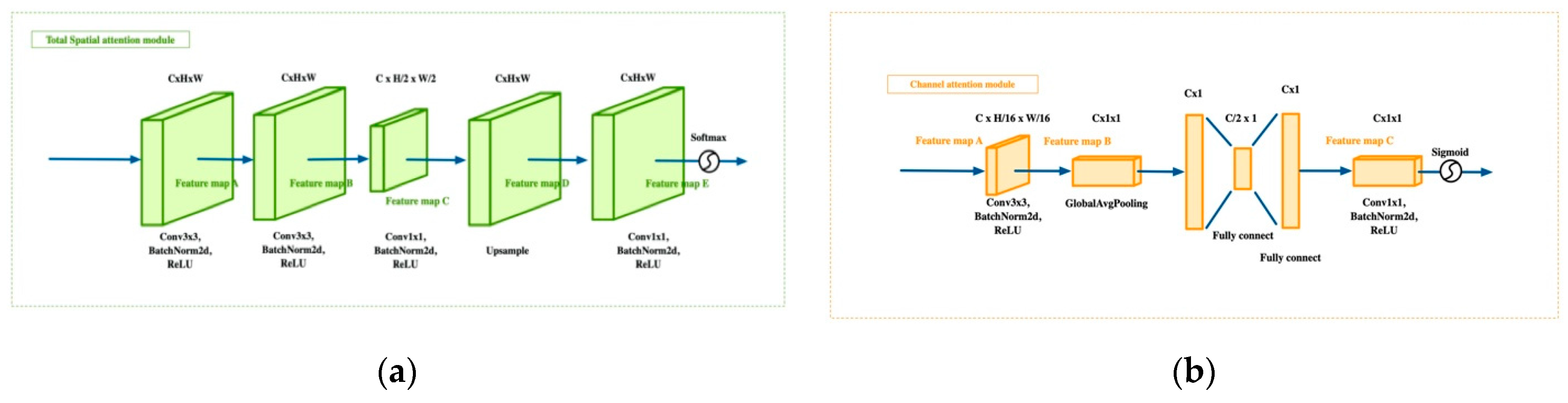
The structure of the total spatial attention module is illustrated in Figure 3a. The input data are the remote sensing image, I ∊ R^4×H×W, which is the same as the input data in ResNet. Input I first passes through the layers conv3×3, BN [49], and ReLU, with channel number C, to generate the feature map, A ∊ R^C×H×W. Then, A is fed into the conv1×1, BN, and ReLU layers to obtain the next feature map, B ∊ R^1×H×W. Feature map B passes through another conv1×1 layer to generate the feature map, C ∊ R^1×H×W. Finally, a sigmoid function is used to get the spatial attention weighting factor, W_s∊ R^H×W. The process is as follows:

A = ReLU(BN(Conv^3×3(I_o)))

(1)

B = ReLU(BN(Conv^1×1(A)))

(2)

ReLU = max(Input, 0)

(3)

C = Conv^1×1(B)

(4)

W_s= Sigmoid(C)

(5)

where I_o denotes the original remote sensing image, and A, B, and C are the corresponding feature maps in Figure 3a. In this way, each value, w_s in W_s, is between 0 and 1. This can be regarded as the weight of each corresponding pixel in the original image, reflecting the pixel’s relative importance. This simple method makes it possible to generate a position weight with the same width and height as the original image, with the network enhancing the pixel level local feature extraction ability with almost no increase in computation. Thus, more effective remote sensing scene features can be extracted, thereby improving the classification performance.

3.3. Channel Attention Module

There are some commonplace problems in remote sensing image datasets. These include the uneven distribution of samples and the varying complexity of different kinds of land cover. When a model is trained, as the network deepens, the semantic information becomes increasingly sophisticated. Each channel in the final advanced semantic features can be seen as a summary of different types of land cover. We introduced a channel attention module(CAM) to enhance the feature channels with similar values occurring in the same image location. If the same position in an image has similar values for different channels, it means that there may be at least two types of feature, with little or no difference between them. The output of the CAM aims to make the relationship between similar channels more obvious. The CAM can capture different kinds of important information in a remote sensing image relating to different channels in the high-level semantic feature map. This facilitates the extraction of key features, refining the balance in the adaptive feature extraction. The input for the CAM is the feature map, F₁. This contains the highest-level semantic features in the whole model.

The structure of the CAM is illustrated in Figure 3b. The input data are the feature map, F₁ ∊ R^{512×H/4×W/4}. The input, F₁, first passes through a 3 × 3 convolutional layer, a BN layer, and a ReLU layer, with the channel number, C, to generate the feature map A ∊ R^C×H×W. Then, Global Average Pooling is used to obtain the feature map, B ∊ R^C×1×1. Then, B is fed into a 1 × 1 convolutional layer to get the feature map, C ∊ R^C×1×1. Finally, we use a sigmoid function to get the channel attention weighting factor, W_c ∊ R^C×1×1. The process can be summarized as follows:

A = ReLU(BN(Conv^3×3(F₁)))

(6)

B = AvgPool(A)

(7)

C = Conv^1×1(B)

(8)

W_c= Sigmoid(C)

(9)

where F₁ is the corresponding feature map in Figure 2; and A, B, and C are the corresponding feature maps in Figure 3a. As with W_s, each value in W_c is between 0 and 1. This can be regarded as the weight of each category, which reflects the feature extraction difficulty. By using this simple method to generate channel weights, the network can focus on more complex types of feature extraction, reduce the redundant information, and improve the land cover type classification.

3.4. Feature Aggregation

By using the above modules, the important information in high-resolution remote sensing images can be extracted more effectively. To make full use of the contextual information, the features are aggregated after the attention weights have been applied. This involves multiplying the output of the two modules (W_s and W_c) and the feature map, F₂ (the PSP-Net output in our example), by the corresponding elements to get two feature maps of the same size, C × H × W. One is the feature map after application of the channel attention weight, F_c. The other is the feature map after application of the spatial attention weight, F_s. The feature aggregation is completed by summing the corresponding elements in F_c and F_s. It should be emphasized that the two attention modules are very simple and can be directly used in any segmentation model. They do not significantly increase the computational load, but they can significantly improve a network’s performance.

4. Experiments

In this section, we first introduce the Gaofen Image Dataset (GID) and explain how the model was implemented. Then, we present how a comprehensive experiment was conducted on the GID dataset to evaluate our proposed method and to compare its semantic segmentation performance against other state-of-the-art algorithms.

4.1. Dataset

4.1.1. Dataset Description

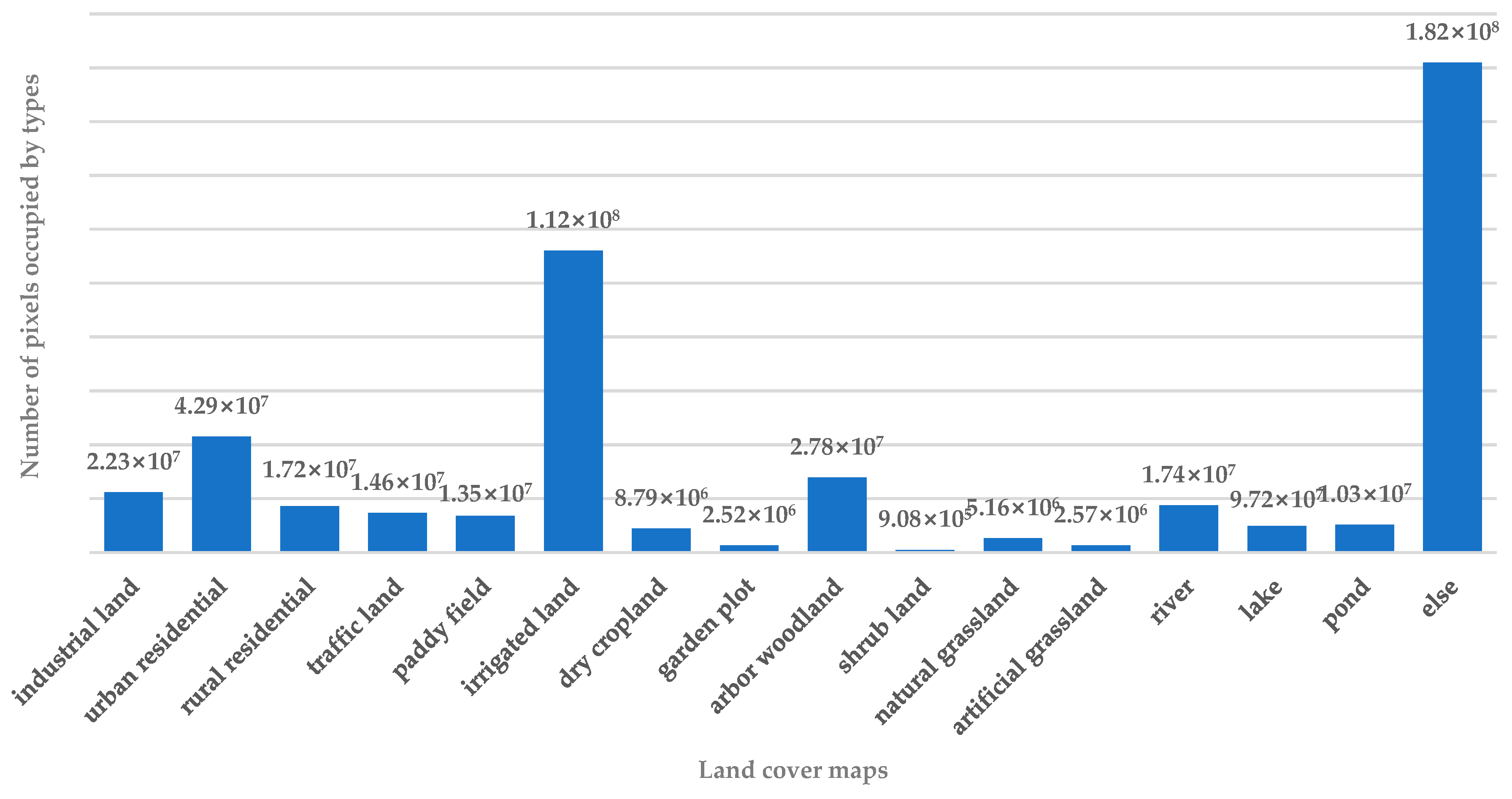
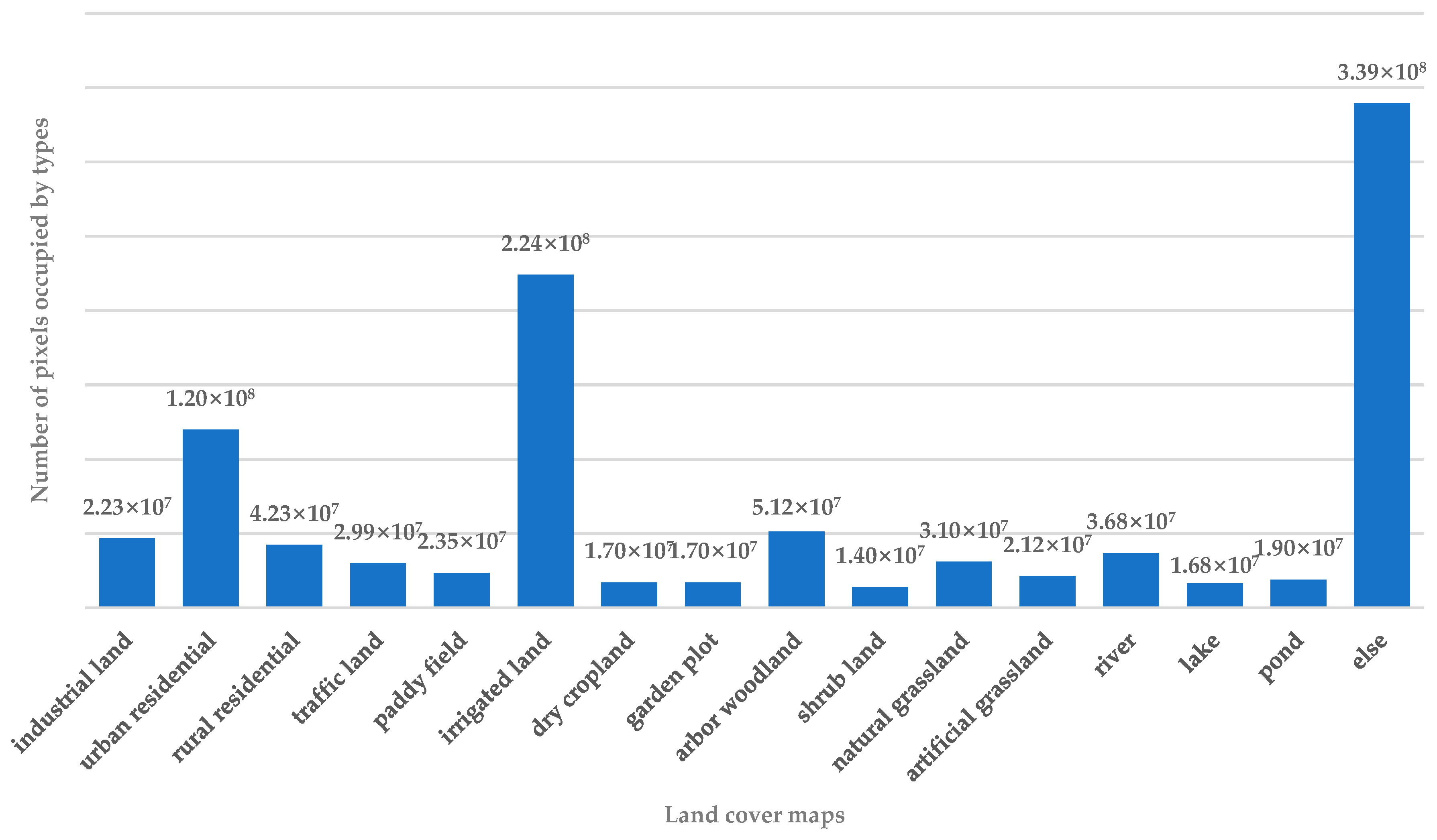
The high-resolution image dataset, GID [26], is a large-scale land cover dataset. It was constructed from GF-2 satellite images. As a result of its large coverage, wide distribution, and high spatial resolution, it has a number of advantages over existing land cover datasets. GF-2 is the highest resolution civil terrestrial observation satellite in China at present, so the image clarity of the dataset is exceptional. The categories covered by the dataset are also both varied and typical, so the characterization of the land cover types is representative of the distribution of the land cover in most parts of China. At the same time, the complexity of the land cover types make the dataset especially valuable for research. The GID dataset consists of two parts: a large-scale classification set and a fine-grained land cover classification set. The large-scale classification set contains 150 GF-2 images annotated at pixel level. The fine-grained classification set consists of 30,000 multi-scale image blocks and 10 pixel level annotated GF-2 images. We deliberately chose to use the GID dataset with 16 kinds of land cover, which are more difficult to train. Each image is 6800 px × 7200 px, with 4 NirRGB channels and high-quality pixel-level labels for the 16 types of land cover. The 16 types of land cover are as follows: industrial land; urban residential; rural residential; traffic land; paddy field; irrigated land; dry cropland; garden plot; arbor woodland; shrub land; natural grassland; artificial grassland; river; lake; pond; and other categories. Figure 4 shows the distribution of the types of land cover.

4.1.2. Dataset Preprocessing

Due to the uneven distribution of the different types of land cover in the GID dataset and the fact that the images are very large, the dataset needed to be preprocessed, so that the training could be more effective. First of all, we manually cropped the 10 images to 1000 px × 1000 px to serve as a validation set, keeping the change in the distribution as small as possible. The reason for selecting the validation set was that our method was a full convolution network (FCN), so it was not sensitive to the size of the input image. Moreover, the size of remote sensing images are often very large, so we chose a larger size image to verify. Manual selection can also ensure a balanced distribution. The distribution of the types of land cover in the validation set is shown in Figure 5.

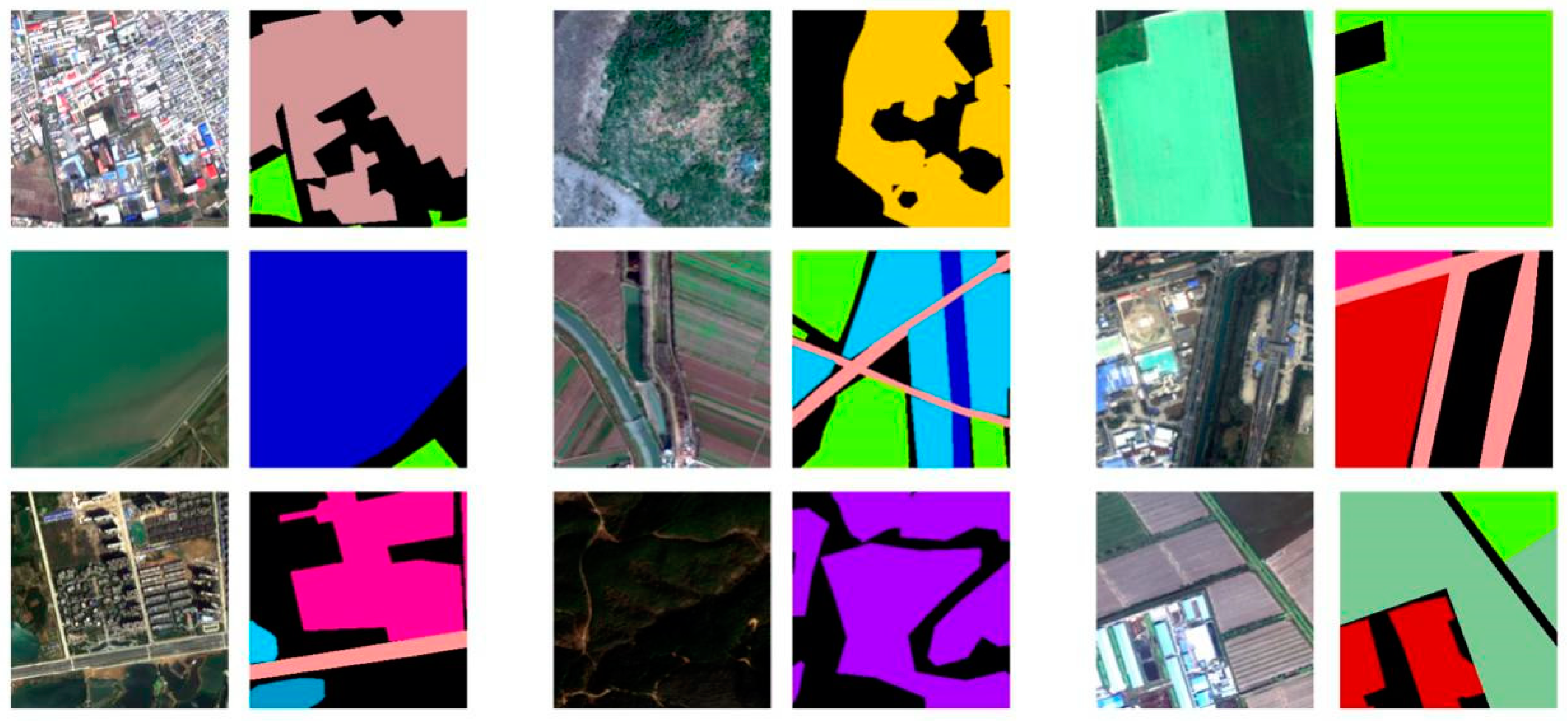
After removing the validation set from the GID dataset, 15,000 images were randomly cropped from the original images to 256 px × 256 px to create a training set. As there was an uneven distribution of different types of land cover, we cropped images with the lowest GID land cover distribution, such as garden plots and artificial grassland from the original images, giving about nine images of different sizes. Then, 1000 256 px × 256 px images were randomly cropped from these nine images and added to the training set to improve the distribution. Thus, the final training set was made up of 16,000 images with a size of 256 px × 256 px, as shown in Figure 6. Figure 7 shows the training set’s distribution. We did not use a test set, as the size of the dataset was too small. Although there are 16,000 images in the training dataset, they are randomly cropped from the rest of the GID dataset. Therefore, there is an overlap between the pictures of the training set. This operation itself is a data enhancement process and would be difficult to train because it would take up too much memory.

4.1.3. Data Augmentation

High-resolution remote sensing images can very easily cause network overfitting because it is hard to obtain a sufficient number of labeled images. The limited number of types in the small GID dataset also made the network training more difficult. Therefore, a data augmentation strategy was employed to enhance the generalizability of the network. We used Albumentations (https://github.com/albumentations-team/albumentations) to augment the dataset and applied the horizontalflip, verticalflip, randomrotate90, and transform functions to enrich the training dataset. This also gave the features extracted from the network rotation invariance. Elastictransform, blur, and cutout were also used for every image during the training to suppress the likelihood of the network capturing insignificant features. The probability for all of the above operations was 0.5.

4.2. Implementation Details

We used the pixel accuracy (Acc), mean IoU, and F1-score as performance evaluation metrics for the semantic segmentation results. Pixel accuracy is the number of correctly classified pixels divided by the total number of pixels in the image. It can be calculated as follows:

$$\mathrm{Acc}=\frac{{\displaystyle {\sum }_{\mathrm{i}=0}^{\mathrm{k}}}{\mathrm{p}}_{\mathrm{ii}}}{{\displaystyle {\sum }_{\mathrm{i}=0}^{\mathrm{k}}}{{\displaystyle \sum }}_{\mathrm{j}=0}^{\mathrm{k}}{\mathrm{p}}_{\mathrm{ij}}}$$

(10)

where k is the number of foreground categories; p_ii is the number of pixels predicted correctly; and p_ij represents a pixel that belongs to class i but that is predicted to belong to class j.

With regard to semantic segmentation, the mean IoU calculates the mean intersection-over-union of two sets with the same kind of category: the ground truth and the predicted segmentation. This is a valuable measure for establishing segmentation performance. The results fall in the range of 0 to 1, with a higher value indicating a better segmentation performance. The mean IoU can be calculated as follows:

$$\mathrm{MIoU}=\frac{1}{\mathrm{k}+1}{\displaystyle {\sum }_{\mathrm{i}=0}^{\mathrm{k}}}\frac{{\mathrm{p}}_{\mathrm{ii}}}{{{\displaystyle \sum }}_{\mathrm{j}=0}^{\mathrm{k}}{\mathrm{p}}_{\mathrm{ij}}+{{\displaystyle \sum }}_{\mathrm{j}=0}^{\mathrm{k}}{\mathrm{p}}_{\mathrm{ji}}-{\mathrm{p}}_{\mathrm{ii}}}$$

(11)

where k is the number of foreground categories; p_ii is the number of pixels predicted correctly; and p_ij and p_ji are the false positive and false negative interpretations.

Another indicator that is used is the F1-score. The F1-score is the weighted harmonic mean of the precision and recall. The F1-score and recall can be obtained as follows:

$${\mathrm{F}}_1 = 2\times \frac{\mathrm{Acc}\times \mathrm{Rec}}{\mathrm{Acc}+\mathrm{Rec}}$$

(12)

$$\mathrm{Rec} = \frac{{{\displaystyle \sum }}_{\mathrm{i}=0}^{\mathrm{k}}{\mathrm{p}}_{\mathrm{ii}}}{{{\displaystyle \sum }}_{\mathrm{i}=0}^{\mathrm{k}}{\mathrm{p}}_{\mathrm{ii}}+{{\displaystyle \sum }}_{\mathrm{i}=0}^{\mathrm{k}}{{\displaystyle \sum }}_{\mathrm{j}=0}^{\mathrm{k}}{\mathrm{p}}_{\mathrm{ji}}}$$

(13)

where Acc is the pixel accuracy mentioned above; p_ii is the number of pixels predicted correctly; and p_ji denotes the false negative interpretations.

After augmenting the training set using the above method, we set the training period to 100 epochs for all of the experiments and employed an apex to obtain semi-precise training. We used a weight decay of 0.00001 and a momentum of 0.9. All of the backbones of the model were set to Resnet50, which was pretrained on ImageNet to facilitate ablation experiments. Cross-Entropy Loss was used at the end of the model to supervise the final results. This can be calculated as follows:

$$\mathrm{CELoss}=-{{\displaystyle \sum }}_{\mathrm{i}=0}^{\mathrm{n}}{\mathrm{p}}_{\mathrm{gt}}({\mathrm{p}}_{\mathrm{i}})\log ({\mathrm{p}}_{\mathrm{pre}}({\mathrm{p}}_{\mathrm{i}}))$$

(14)

where n is the total number of pixels; p_gt is the ground truth of pixel p_i; and p_pre is the prediction for pixel p_i. The base learning rate was set to 0.15 and decreased to 0.00001 through cosine annealing until the end of the training was achieved. We used the Ubuntu 18.04 system for the experiment and the GPU was an NVIDIA RTX2080TI. The experiment was implemented by using Pytorch and was optimized by adopting a stochastic gradient descent (SGD) approach.

4.3. Results

4.3.1. Ablation Study of Total Spatial Attention Module-Related Improvements

Numerous approaches have used channel and spatial attention modules in recent years [20,22,26]. Most use the feature map, F₁, as input (see Figure 2). In our total spatial attention module (TSAM), the basic idea of a spatial attention module is modified by moving its location and simplifying the structure to ensure the method’s overall simplicity. The part to be played by a CAM is well-established, so there is no need to repeat studies of the CAM here. Therefore, our experiments primarily focused on the potential improvements arising from using a TSAM.

• Experiment 1: Effect of High-Level Semantic Information on the TSAM

As the TSAM extracts features from the original image, it is possible that a lack of advanced semantic information might affect its effectiveness. To assess this possibility, we extracted a spatial weighting factor matrix from the backbone and fused it with the TSAM’s output to increase the high-level semantic information. Then, a method without any high-level spatial attention (HLSA) was compared with methods that use high-level spatial attention in various ways. We used PSP-Net for the experiment (DPA-PSP-Net) because DPA-Net can be appended to any network. The experiment showed that using the TSAM without HLSA for the original image was sufficiently effective. It delivered results of 82.75% for Acc and 67.92% for the mean IoU. HLSA did not improve the network performance, so we did not employ it. The experimental results are shown in

Table 1. Performance comparison between different DPA-PSP-Net structures.

Method	with HLSA	without HLSA	Acc (%)	Mean IoU (%)
DPA-PSPNet	√		0.8277	0.6792
DPA-PSPNet		√(concat)	0.8235	0.6772
DPA-PSPNet		√(add)	0.8258	0.667

.

• Experiment 2: Effect of the TSAM Location

As a network deepens, the feature map becomes smaller, and the spatial information decreases. This was the basis of our reasoning that it would be more effective to capture the spatial information from the original image. To verify this assumption, we calculated the TSAM for three different locations in the model: at the beginning, in the middle, and at the end of the backbone. ResNet consists of five blocks in series. We chose the original image, the 3rd block’s ResNet output and the 5th block’s ResNet output as the TSAM input. The feature maps corresponding to the blocks in ResNet were 1, 1/4, and 1/8 times the size of the original image. As shown in

Table 2. Performance comparison for the total spatial attention module (TSAM) at different positions.

Method	Input of TSAM	Acc (%)	Mean IoU (%)
DPA-PSP-Net	5th block’s ResNet output	82.44	67.09
DPA-PSP-Net	3rd block’s ResNet output	82.55	67.32
DPA-PSP-Net	Original image	82.77	67.92

, the performance of the TSAM improved in line with an increase in the input size, confirming that our initial conjecture was correct.

• Experiment 3: Effect of the Depth of the TSAM

To assess the effect of the depth of the TSAM, we tested different numbers of parameters to find the most efficient structure. We only changed the number of layers before the layer that makes up the feature map’s channel 1. In other words, we kept the last two 1 × 1 convolutions and increased or decreased the number of 3 × 3 convolutions. The experimental results show that the performance was most effective when there were three layers in the TSAM.

Table 3. Performance comparison for TSAMs with different depths.

Position of TSAM	Depth of TSAM	Acc (%)	Mean IoU (%)
Original image	[Conv1×1] × 2	82.14	66.97
Original image	[Conv3×3] × 1, [Conv1×1] × 2	82.77	67.92
Original image	[Conv3×3] × 2, [Conv1×1] × 2	82.19	67.55
Original image	[Conv3×3] × 3, [Conv1×1] × 2	82.5	67.71

shows the results for models using different numbers of layers.

4.3.2. Ablation Study for Both Attention Modules

In order to assess any potential differences between the effect of the two modules on improving the remote sensing semantic segmentation performance, we conducted experiments with different combinations. The results are shown in

Table 4. Ablation study for different attention module combinations.

Model	CAM	TSAM	Acc (%)	Mean IoU (%)	F1-Score (%)
PSP-Net			81.60	65.38	63.97
DPA-PSP-Net	√		81.56	66.90	71.45
DPA-PSP-Net		√	81.30	67.37	70.04
DPA-PSP-Net	√	√	82.75	67.92	72.56

.

Table 4 makes evident the performance improvements brought about by using both the CAM and the TSAM. Compared with a baseline PSP-Net, applying a CAM delivered a mean IoU result of 66.90% and an F1-score of 71.45%, which amounts to a 1.52% and 7.48% improvement, respectively. Employing just a TSAM increased the mean IoU to 67.37% and F1-score to 6.07%. However, the biggest performance improvement came from using both modules together. When we integrated the CAM and TSAM, the mean IoU result was 67.92%, which was 2.54% higher than the baseline. The F1-score result was 72.56%, which was 8.59% higher than the baseline. These experimental results confirm that the dual path attention approach with two modules is a more effective strategy for improving the performance of semantic segmentation models on remote sensing images.

We also considered the feasibility of a Squeeze-and-Excitation(SE) operation, so we added SE operations to CAM and TSAM for comparative experiments. The structure is illustrated in Figure 8. For TSAM, we add a convolutional layer to reduce its size to H/2 × W/2. Then, we used an upsampling operation to restore it to its original size. For CAM, we used a fully connected layer to reshape its size to C/2 × 1 and restore it. The output of TSAM was also changed to 16 channels, i.e., the number of channels and the number of land cover types were the same. The experimental results are shown in

Table 5. DPA-Net performance using the structure in Figure 8.

Method	SE, 16 Channel	1 Channel	Acc (%)	Mean IoU (%)	F1-Score (%)
DPA-UNet	√		82.72	66.58	63.73
DPA-UNet		√	82.78	67.07	65.03
DPA-PSPNet	√		82.70	66.71	65.75
DPA-PSPNet		√	82.75	67.92	72.56
DPA-DeepLab	√		81.58	66.93	67.10
DPA-DeepLab		√	82.83	67.37	67.31

.

We noticed that the performance of TSAM using Squeeze-and-Excitation operations was not always as good as expected. The structure of the attention module also became more complex, although its performance was not better. The mean IoU results for the SE operations were also lower than the results using our method by 0.59%, 1.21%, and 0.44% for U-Net, PSP-Net, and Deeplab V3+, respectively. The F1-score results for the SE operations were lower than those produced by our proposed method by 1.30%, 6.81%, and 0.21%, respectively. This may be because the function of the Squeeze-and-Excitation operation is to remove redundant information. However, our CAM focuses on the features of categories and is no longer able to remove redundancy. The purpose of setting the TSAM input as the original image is to have better resolution, retain better state features, and provide a better positioning function. Therefore, the Squeeze-and-Excitation operation may not be best applied to a TSAM.

4.3.3. Comparison with Different Models

In view of the small amount of GID data, we used augmentation to offset the potential problem of network overfitting. To verify the validity of our chosen augmentation method, we conducted experiments where we trained DPA-Net on the U-Net, PSP-Net, and DeepLab V3+ semantic segmentation models, using the original dataset and the augmented dataset. The results are shown in

Table 6. DPA-Net performance using the original dataset and the augmented dataset.

Method	Acc (%)	Mean IoU (%)	F1-Score (%)
DPA-UNet	81.63	65.88	57.41
DPA-UNet Aug	82.78	67.07	65.75
DPA-PSP-Net	81.38	65.45	65.43
DPA-PSP-Net Aug	82.75	67.92	72.56
DPA-DeepLab	80.84	64.95	61.49
DPA-DeepLab Aug	82.83	67.37	67.31

.

The results indicate that the augmentation strategy we employed was effective. The semantic segmentation mean IoU increased to 67.07%, 67.92%, and 67.37% for U-Net, PSP-Net, and DeepLab V3+, respectively. The F1-score increased to 65.75%, 72.56%, and 67.31% for the above techniques, respectively. This suggests that augmentation strategies can enhance the scope for network generalization by enriching the data.

To verify the effectiveness of our method in relation to actual remote sensing image segmentation tasks, we compared it against more mainstream methods based on self-attention mechanisms. These methods were Non-Local NN, SE-Net, CBAM, and DA-Net. The results of the experiment are shown in

Table 7. Mean IoU for each category of the different self-attention models.

Class	Non-Local NN	SE-Net	CBAM	DA-Net	DPA-PSP-Net
in-l 1	35.37	32.35	41.17	35.03	32.37
ur 2	60.09	58.91	61	52.29	59.27
rr 3	71.14	69.85	70.16	63.75	71.05
tl 4	82.35	85.06	81.08	82.39	88.01
pf 5	87.59	87.41	81.33	85.23	87.4
ir-l 6	57.32	55.6	54.9	56.21	57.7
dc 7	63.6	73.22	63.67	50.81	69.95
gp 8	49.13	44.58	49.8	47.87	67.44
aw 9	57.34	57.49	55.21	53.97	52.13
sw 10	0	25.5	4.93	30.6	0
ng 11	66.71	66.73	69.54	72.99	71.59
ag 12	78.97	85.81	82.99	73.96	87.63
river	81.22	77.76	79.22	83.96	86.39
lake	90.7	88.23	89.18	86.78	92.78
pond	85.31	86.59	88.81	89.23	88.5
else	74.12	74.61	74.32	69.59	74.52
mean	65.06	66.86	65.45	64.67	67.92

¹ industrial land, ² urban residential, ³ rural residential, ⁴ traffic land, ⁵ paddy field, ⁶ irrigated land, ⁷ dry cropland, ⁸ garden plot, ⁹ arbor woodland, ¹⁰ shrub woodland, ¹¹ natural grassland, ¹² artificial grassland.

and

Table 8. F1-score for each category of the different self-attention models.

Class	Non-Local NN	SE-Net	CBAM	DA-Net	DPA-PSP-Net
in-l 1	52.26	48.88	58.33	51.89	48.55
ur 2	75.07	74.14	75.78	68.67	74.52
rr 3	83.14	82.25	82.46	77.86	83.01
tl 4	90.32	91.93	89.55	90.33	93.60
pf 5	93.38	93.28	89.70	92.02	93.31
ir-l 6	72.88	71.47	70.88	71.96	73.06
dc 7	77.75	84.54	77.80	67.39	82.46
gp 8	65.89	61.68	66.49	64.75	80.06
aw 9	72.89	73.00	71.14	70.10	67.55
sw 10	0	40.63	9.40	46.87	0.00
ng 11	80.03	80.05	81.97	84.39	83.39
ag 12	88.25	92.36	90.71	85.03	93.52
river	89.64	87.49	88.40	91.28	92.70
lake	95.12	93.75	94.28	92.93	96.21
pond	92.08	92.81	94.07	94.31	93.95
else	85.14	85.46	85.27	82.07	85.44
macro	65.09	66.74	60.57	62.01	72.56

¹ industrial land, ² urban residential, ³ rural residential, ⁴ traffic land, ⁵ paddy field, ⁶ irrigated land, ⁷ dry cropland, ⁸ garden plot, ⁹ arbor woodland, ¹⁰ shrub woodland, ¹¹ natural grassland, ¹² artificial grassland.

.

The experimental results show that DPA-PSP-Net provided the most effective semantic segmentation. SE-Net was the next most effective. The mean IoUs for the supposedly stronger CBAM and DA-Net were only 65.45% and 64.67%, respectively. Non-local NN and SE-Net had better F1-scores. However, they were still lower than that of DPA-PSP-Net. This confirms that the segmentation of remote sensing images is different from normal scene segmentation, so, DPA-PSP-Net may have an advantage over existing methods.

To further assess the effectiveness of the proposed method, we compared the mean IoU and F1-score for each type of land cover when using the three different models, U-Net, PSP-Net, and DeepLab V3+, with or without DPA-Net.

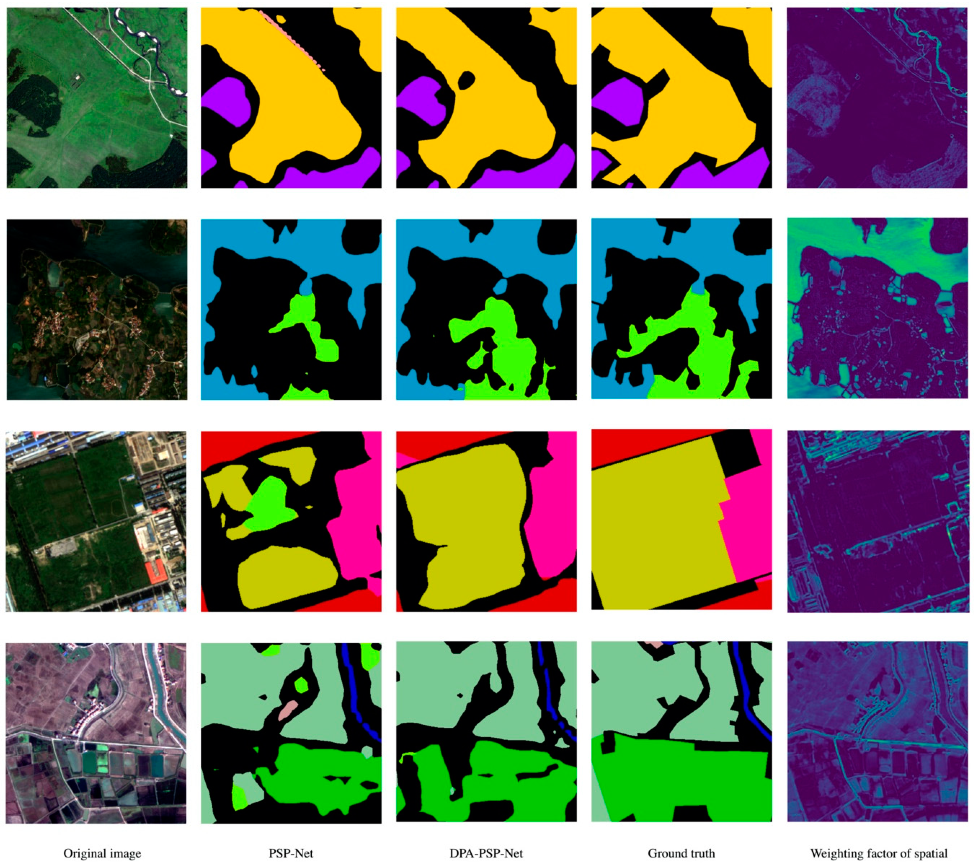
As shown in

Table 9. Mean IoU for each category using different models.

Class	UNet	DPA-UNet	PSP-Net	DPA-PSP-Net	DeepLab V3+	DPA-DeepLab
in-l 1	29.06	42.48	32.15	32.37	29.22	50.83
ur 2	59.16	60.88	57.04	59.27	56.49	61.54
rr 3	74.05	73.65	70.63	71.05	71.17	73.62
tl 4	85.66	88.43	87.86	88.01	83.48	84.89
pf 5	88.35	86.23	86.49	87.4	87.03	82.53
ir-l 6	57.53	57.83	54.01	57.7	60.09	58.82
dc 7	68.45	69.51	66.12	69.95	67.88	62.37
gp 8	38.82	47.09	49.01	67.44	43.4	47.79
aw 9	60.32	60.31	59.31	52.13	55.66	57.29
sw 10	2.03	1.07	0	0	2.45	0
ng 11	71.9	72.9	69.95	71.59	71.66	71.84
ag 12	80.4	79.62	80.52	87.63	82.3	84.67
river	86.06	78.98	82.35	86.39	86.68	86.32
lake	94.42	93.21	91.25	92.78	94.72	92.32
pond	87.63	86.46	85.96	88.5	89.33	88.7
else	75.91	74.47	73.48	74.52	75.19	74.43
mean	66.23	67.07	65.38	67.92	66.05	67.37

¹ industrial land, ² urban residential, ³ rural residential, ⁴ traffic land, ⁵ paddy field, ⁶ irrigated land, ⁷ dry cropland, ⁸ garden plot, ⁹ arbor woodland, ¹⁰ shrub woodland, ¹¹ natural grassland, ¹² artificial grassland.

and

Table 10. F1-score for each category using the different models.

Class	UNet	DPA-UNet	PSP-Net	DPA-PSP-Net	DeepLab V3+	DPA-DeepLab
in-l 1	45.04	59.63	71.36	48.55	45.23	67.40
ur 2	74.34	75.69	68.46	74.52	72.20	76.19
rr 3	85.09	84.83	76.18	83.01	83.14	84.80
tl 4	92.28	93.86	87.26	93.60	91.00	91.83
pf 5	93.81	92.61	93.04	93.31	93.07	90.43
ir-l 6	73.04	73.28	71.79	73.06	75.07	74.07
dc 7	81.27	82.02	77.52	82.46	80.86	76.83
gp 8	55.93	64.03	60.18	80.06	60.53	64.67
aw 9	75.24	75.24	72.42	67.55	71.52	72.84
sw 10	3.97	2.11	27.65	0.00	4.79	0.00
ng 11	83.66	84.33	81.83	83.39	83.49	83.61
ag 12	89.13	88.65	89.25	93.52	90.29	91.69
river	92.51	88.25	89.92	92.70	92.86	92.66
lake	97.13	96.49	93.44	96.21	97.29	96.01
pond	93.41	92.74	89.98	93.95	94.37	94.01
else	86.30	85.37	83.21	85.44	85.84	85.34
macro	62.82	65.03	63.97	72.56	67.00	67.31

¹ industrial land, ² urban residential, ³ rural residential, ⁴ traffic land, ⁵ paddy field, ⁶ irrigated land, ⁷ dry cropland, ⁸ garden plot, ⁹ arbor woodland, ¹⁰ shrub woodland, ¹¹ natural grassland, ¹² artificial grassland.

, every model performed better with DPA-Net than it did on its own. Note in particular that although PSP-Net had lower mean IoU results than U-Net and DeepLab V3+ on its own, DPA-PSP-Net outperformed any other approach. The same is true for the F1-scores. Another point to note is that because the distribution of shrubbery woodland was so small, no network had a good way of capturing its key features, so every approach had poor results. However, this did not change the fact that DPA-Net still improved the segmentation model. Several visual comparisons using PSP-Net as an example are shown in Figure 9.

The output of TSAM is shown in the rightmost column in Figure 9. Although the input of TSAM is the original image, the output does not seem to include a lot of noise. For some position attention modules, such as “lake” in the second row and “dry cropland” in the last row, the details and boundaries are even more clear. These results reveal the effectiveness of the visualized weighting factors of TSAM.

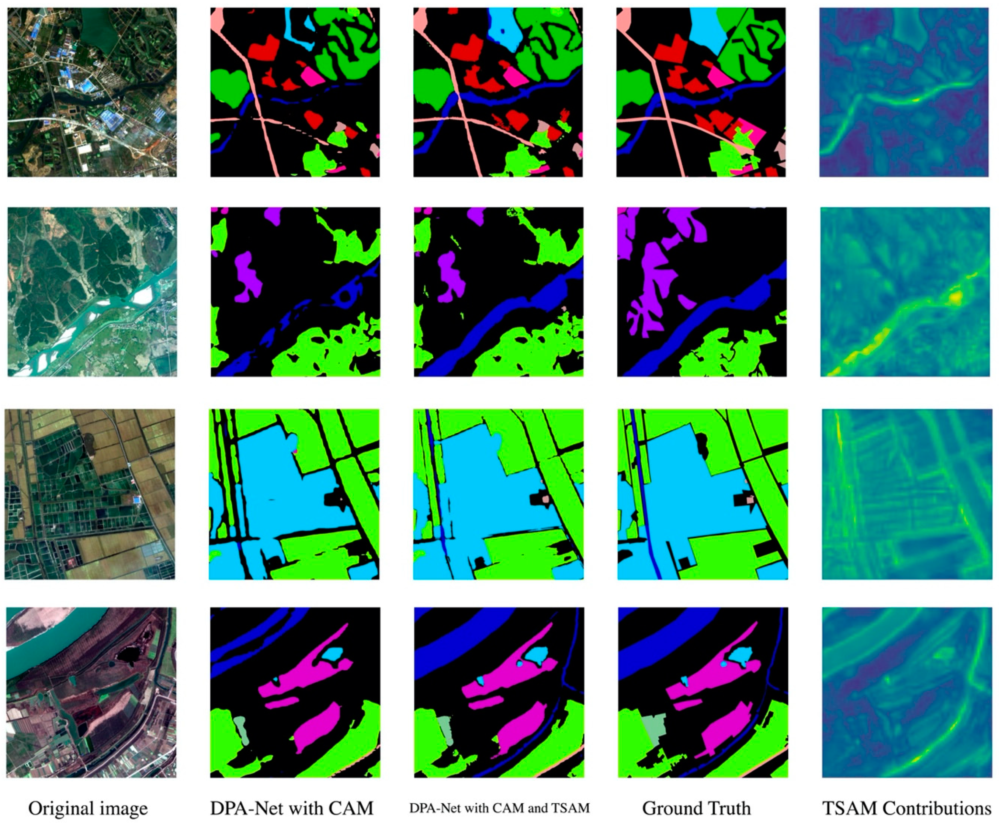
To further assess the contribution made by TSAM to DPA-Net, we visualized the differences in the output of DPA-Net with different forms of attention. We randomly selected a test image as shown in Figure 10. We first compared the output of DPA-Net with just CAM, then with both TSAM and CAM, while saving the output feature maps that passed the softmax function. The size of these two feature maps was (C, H, W). Then, we performed an L1 Norm operation on these two feature maps for the C dimension, yielding a heat map with a size of (1000, 1000). This is shown in the right-hand column of Figure 10.

This heat map shows the difference in output between DPA-Net with TSAM and without TSAM. The brighter the highlight, the greater the contribution of TSAM. In the images, we can see that the river and the lake areas are relatively pronounced. This means that the contribution of TSAM was especially significant in these regions. This heat map makes the contribution of TSAM to the overall prediction evident.

We also counted the Multiplication and Accumulation (MAC) results for DPA-Net and the number of parameters required, and then, we compared them with the original U-Net, PSP-Net, and DeepLab V3+ models. As can be seen in

Table 11. Multiplication and Accumulation (MAC) results and number of parameters for different models.

	U-Net	DPA-UNet	PSP-Net	DPA-PSPNet	DeepLab V3+	DPA-DeepLab
MACs(G)	31.946	32.016	23.035	23.258	43.499	43.57
Params(M)	28.118	28.193	31.968	32.045	29.98	30.055

, the MAC results only increased by 0.07G, 0.223G, and 0.069G, respectively, across the three models, and the number of parameters only increased by 0.075M, 0.077M, and 0.075M, respectively. This shows that compared with the original method, DPA-Net only increases the memory footprint by a small amount.

5. Conclusions

In this paper, we have proposed a Dual Path Attention Network (DPA-Net) for the semantic segmentation of remote sensing images. It can be used with any segmentation model without having any significant impact on the memory footprint or number of parameters. A remote sensing image is first processed via the backbone and a total spatial attention module to obtain a feature map and spatial weighting factor. Then, a CAM is calculated from the feature map to get the channel weighting factor. Finally, the output of the segmentation model is multiplied by the spatial weighting factor and channel weighting factor separately to get two feature maps that capture different aspects of the features. Then, these two feature maps are fused to obtain the final DPA-Net output. The proposed network was tested and found to improve the performance of various state-of-the-art segmentation models on the GID dataset. We believe the performance can be further improved by refining the structure of the two path attention modules, so this will be the focus of our future work.

References

- Napoletano, P. Visual descriptors for content-based retrieval of remote-sensing images. Int. J. Remote Sens. 2017, 39, 1343–1376. [Google Scholar] [CrossRef] [Green Version]
- Yang, Y.; Newsam, S. Geographic Image Retrieval Using Local Invariant Features. IEEE Trans. Geosci. Remote Sens. 2012, 51, 818–832. [Google Scholar] [CrossRef]
- Sun, W.; Wang, R. Fully Convolutional Networks for Semantic Segmentation of Very High Resolution Remotely Sensed Images Combined With DSM. IEEE Geosci. Remote Sens. Lett. 2018, 15, 474–478. [Google Scholar] [CrossRef]
- Panboonyuen, T.; Jitkajornwanich, K.; Lawawirojwong, S.; Srestasathiern, P.; Vateekul, P. Semantic Segmentation on Remotely Sensed Images Using an Enhanced Global Convolutional Network with Channel Attention and Domain Specific Transfer Learning. Remote Sens. 2019, 11, 83. [Google Scholar] [CrossRef] [Green Version]
- Liu, Y.; Fan, B.; Wang, L.; Bai, J.; Xiang, S.; Pan, C. Semantic labeling in very high resolution images via a self-cascaded convolutional neural network. ISPRS J. Photogramm. Remote Sens. 2018, 145, 78–95. [Google Scholar] [CrossRef] [Green Version]
- Wang, H.; Wang, Y.; Zhang, Q.; Xiang, S.; Pan, C. Gated convolutional neural network for semantic segmentation in high-resolution images. Remote Sens. 2017, 9, 446. [Google Scholar] [CrossRef] [Green Version]
- Zhu, X.X.; Tuia, D.; Mou, L.; Xia, G.S.; Zhang, L.; Xu, F.; Fraundorfer, F. Deep learning in remote sensing: A comprehensive review and list of resources. IEEE Geosci. Remote Sens. Mag. 2017, 5, 8–36. [Google Scholar] [CrossRef] [Green Version]
- Panboonyuen, T.; Vateekul, P.; Jitkajornwanich, K.; Lawawirojwong, S. An Enhanced Deep Convolutional Encoder-Decoder Network for Road Segmentation on Aerial Imagery. In Recent Advances in Information and Communication Technology Series; Springer: Cham, Switzerland, 2017; Volume 566. [Google Scholar]
- Wang, S.; Guan, Y.; Shao, L. Multi-Granularity Canonical Appearance Pooling for Remote Sensing Scene Classification. IEEE Trans. Image Process. 2020, 29, 5396–5407. [Google Scholar] [CrossRef] [Green Version]
- Fang, J.; Yuan, Y.; Lu, X.; Feng, Y. Robust Space–Frequency Joint Representation for Remote Sensing Image Scene Classification. IEEE Trans. Geosci. Remote Sens. 2019, 57, 7492–7502. [Google Scholar] [CrossRef]
- He, N.; Fang, L.; Li, S.; Plaza, J.; Plaza, J. Remote Sensing Scene Classification Using Multilayer Stacked Covariance Pooling. IEEE Trans. Geosci. Remote Sens. 2018, 56, 6899–6910. [Google Scholar] [CrossRef]
- Chen, Y.; Fan, R.; Yang, X.; Wang, J.; Latif, A. Extraction of Urban Water Bodies from High-Resolution Remote-Sensing Imagery Using Deep Learning. Water 2018, 10, 585. [Google Scholar] [CrossRef] [Green Version]
- Rezaee, M.; Mahdianpari, M.; Zhang, Y.; Salehi, B. Deep Convolutional Neural Network for Complex Wetland Classification Using Optical Remote Sensing Imagery. IEEE J. Sel. Top. Appl. Earth Obs. Remote Sens. 2018, 11, 3030–3039. [Google Scholar] [CrossRef]
- Mahdianpari, M.; Salehi, B.; Rezaee, M.; Mohammadimanesh, F.; Zhang, Y. Very Deep Convolutional Neural Networks for Complex Land Cover Mapping Using Multispectral Remote Sensing Imagery. Remote Sens. 2018, 10, 1119. [Google Scholar] [CrossRef] [Green Version]
- Yang, H.; Wu, P.; Yao, X.; Wu, Y.; Wang, B.; Xu, Y. Building Extraction in Very High Resolution Imagery by Dense-Attention Networks. Remote Sens. 2018, 10, 1768. [Google Scholar] [CrossRef] [Green Version]
- Shuai, B.; Zuo, Z.; Wang, B.; Wang, G. Scene Segmentation with DAG-Recurrent Neural Networks. IEEE Trans. Pattern Anal. Mach. Intell. 2018, 40, 1480–1493. [Google Scholar] [CrossRef]
- Wang, X.; Girshick, R.; Gupta, A.; He, K. Non-local Neural Networks. In Proceedings of the IEEE Conference on Computer Vision and Pattern Recognition, Salt Lake City, UT, USA, 18–22 June 2018; pp. 7794–7803. [Google Scholar]
- Liao, X.; He, L.; Yang, Z.; Zhang, C. Video-based Person Re-identification via 3D Convolutional Networks and Non-local Attention. In Proceedings of the Asian Conference on Computer Vision, Perth, Australia, 2–6 December 2018. [Google Scholar]
- Du, Y.; Yuan, C.; Li, B.; Zhao, L.; Li, Y.; Hu, W. Interaction-Aware Spatio-Temporal Pyramid Attention Networks for Action Classification. In Proceedings of the European Conference on Computer Vision (ECCV), Munich, Germany, 8–14 September 2018; pp. 388–404. [Google Scholar]
- Woo, S.; Park, J.; Lee, J.Y.; So Kweon, I. Convolutional Block Attention Module. In Proceedings of the European Conference on Computer Vision (ECCV), Munich, Germany, 8–14 September 2018; pp. 3–19. [Google Scholar]
- Hu, J.; Shen, L.; Albanie, S.; Sun, G. Squeeze-and-Excitation Networks. In Proceedings of the IEEE Conference on Computer Vision and Pattern Recognition, Salt Lake City, UT, USA, 18–22 June 2018; pp. 7132–7141. [Google Scholar]
- Fu, J.; Liu, J.; Tian, H.; Li, Y.; Bao, Y.; Fang, Z.; Lu, H. Dual Attention Network for Scene Segmentation. In Proceedings of the IEEE Conference on Computer Vision and Pattern Recognition, Long Beach, CA, USA, 16–20 June 2019; pp. 3146–3154. [Google Scholar]
- Zhao, H.; Shi, J.; Qi, X.; Wang, X.; Jia, J. Pyramid Scene Parsing Network. In Proceedings of the IEEE Conference on Computer Vision and Pattern Recognition, Honolulu, HI, USA, 21–26 July 2017; pp. 6230–6239. [Google Scholar]
- Ronneberger, O.; Fischer, P.; Brox, T. U-Net: Convolutional Networks for Biomedical Image Segmentation. In Proceedings of the International Conference on Medical Image Computing and Computer-Assisted Intervention, Munich, Germany, 5–9 October 2015; pp. 234–241. [Google Scholar]
- Chen, L.C.; Zhu, Y.; Papandreou, G.; Schroff, F.; Adam, H. Encoder-Decoder with Atrous Separable Convolution for Semantic Image Segmentation. In Proceedings of the European Conference on Computer Vision (ECCV), Munich, Germany, 8–14 September 2018; pp. 833–851. [Google Scholar]
- Tong, X.Y.; Xia, G.S.; Lu, Q.; Shen, H.; Li, S.; You, S.; Zhang, L. Land-Cover Classification with High-Resolution Remote Sensing Images Using Transferable Deep Models. Remote Sens. Environ. 2020, 237, 111322. [Google Scholar] [CrossRef] [Green Version]
- Zhao, X.; Zhang, J.; Tian, J.; Zhuo, L.; Zhang, J. Residual Dense Network Based on Channel-Spatial Attention for the Scene Classification of a High-Resolution Remote Sensing Image. Remote Sens. 2020, 12, 1887. [Google Scholar] [CrossRef]
- Yao, X.; Han, J.; Cheng, G.; Qian, X.; Guo, L. Semantic Annotation of High-Resolution Satellite Images via Weakly Supervised Learning. IEEE Trans. Geosci. Remote Sens. 2016, 54, 3660–3671. [Google Scholar] [CrossRef]
- Cheng, G.; Zhou, P.; Han, J. Learning Rotation-Invariant Convolutional Neural Networks for Object Detection in VHR Optical Remote Sensing Images. IEEE Trans. Geosci. Remote Sens. 2016, 54, 7405–7415. [Google Scholar] [CrossRef]
- Wang, Y.; Zhang, L.; Tong, X.; Zhang, L.; Zhang, Z.; Liu, H.; Xing, X.; Mathiopoulos, P.T. A Three-Layered Graph-Based Learning Approach for Remote Sensing Image Retrieval. IEEE Trans. Geosci. Remote Sens. 2016, 54, 6020–6034. [Google Scholar] [CrossRef]
- Hubert, M.J.; Carole, E. Airborne SAR-efficient signal processing for very high resolution. Proc. IEEE. 2013, 101, 784–797. [Google Scholar]
- Yu, B.; Yang, L.; Chen, F. Semantic segmentation for high spatial resolution remote sensing images based on convolution neural network and pyramid pooling module. IEEE J. Sel. Top. Appl. Earth Obs. Remote Sens. 2018, 11, 3252–3261. [Google Scholar] [CrossRef]
- Singh, A. Review Article Digital change detection techniques using remotely-sensed data. Int. J. Remote Sens. 1989, 10, 989–1003. [Google Scholar] [CrossRef] [Green Version]
- Saxena, R.; Watson, L.T.; Wynne, R.H.; Brooks, E.B.; Thomas, V.A.; Zhiqiang, Y.; Kennedy, R.E. Towards a polyalgorithm for land use change detection. J. Photogramm. Remote Sens. 2018, 144, 217–234. [Google Scholar] [CrossRef]
- Xing, J.; Sieber, R.; Caelli, T. A scale-invariant change detection method for land use/cover change research. J. Photogramm. Remote Sens. 2018, 141, 252–264. [Google Scholar] [CrossRef]
- Long, J.; Shelhamer, E.; Darrell, T. Fully convolutional networks for semantic segmentation. In Proceedings of the IEEE Conference on Computer Vision and Pattern Recognition, Boston, MA, USA, 7–12 June 2015; pp. 3431–3440. [Google Scholar]
- Ding, H.; Jiang, X.; Shuai, B.; Liu, A.Q.; Wang, G. Context contrasted feature and gated multiscale aggregation for scene segmentation. In Proceedings of the IEEE Conference on Computer Vision and Pattern Recognition, Salt Lake City, UT, USA, 18–22 June 2018; pp. 2393–2402. [Google Scholar]
- Lin, G.; Milan, A.; Shen, C.; Reid, I.D. Refinenet: Multi-path refinement networks for high-resolution semantic segmentation. In Proceedings of the IEEE Conference on Computer Vision and Pattern Recognition, Honolulu, HI, USA, 21–26 July 2017; pp. 5168–5177. [Google Scholar]
- Chen, L.-C.; Papandreou, G.; Kokkinos, I.; Murphy, K.; Yuille, A.L. DeepLab: Semantic Image Segmentation with Deep Convolutional Nets, Atrous Convolution, and Fully Connected CRFs. IEEE Trans. Pattern Anal. Mach. Intell. 2018, 40, 834–848. [Google Scholar] [CrossRef]
- Lazebnik, S.; Schmid, C.; Ponce, J. Beyond Bags of Features: Spatial Pyramid Matching for Recognizing Natural Scene Categories. In Proceedings of the 2006 IEEE Computer Society Conference on Computer Vision and Pattern Recognition (CVPR’06), New York, NY, USA, 17–22 June 2006; pp. 2169–2178. [Google Scholar]
- Chen, L.-C.; Papandreou, G.; Schroff, F.; Adam, H. Rethinking atrous convolution for semantic image segmentation. arXiv 2017, arXiv:1706.05587. [Google Scholar]
- Peng, C.; Zhang, X.; Yu, G.; Luo, G.; Sun, J. Large Kernel Matters—Improve Semantic Segmentation by Global Convolutional Network. In Proceedings of the IEEE conference on computer vision and pattern recognition, Honolulu, HI, USA, 21–26 July 2017; pp. 1743–1751. [Google Scholar]
- Mnih, V.; Heess, N.; Graves, A. Recurrent models of visual attention. In Proceedings of the Neural Information Processing Systems, Montréal, QC, Canada, 8–13 December 2014; pp. 2204–2212. [Google Scholar]
- Wang, Q.; Liu, S.T.; Chanussot, J. Scene classification with recurrent attention of VHR remote sensing images. IEEE Trans. Geosci. Remote Sens. 2018, 57, 1155–1167. [Google Scholar] [CrossRef]
- Vaswani, A.; Shazeer, N.; Parmar, N.; Uszkoreit, J.; Jones, L.; Gomez, A.N.; Kaiser, L.; Polosukhin, I. Attention is all you need. In Proceedings of the Conference on Neural Information Processing Systems, Long Beach, CA, USA, 4–9 December 2017; pp. 6000–6010. [Google Scholar]
- Yao, L.; Torabi, A.; Cho, K.; Ballas, N.; Pal, C.; Larochelle, H.; Courville, A. Describing videos by exploiting temporal structure. In Proceedings of the 2015 IEEE International Conference on Computer Vision (ICCV), Santiago, Chile, 7–13 December 2015; pp. 4507–4515. [Google Scholar]
- Kuen, J.; Wang, Z.; Wang, G. Recurrent attentional networks for saliency detection. In Proceedings of the IEEE Conference on Computer Vision and Pattern Recognition (CVPR), Las Vegas, NV, USA, 26 June–1 July 2016; pp. 3668–3677. [Google Scholar]
- He, K.; Zhang, X.; Ren, S.; Sun, J. Deep Residual Learning for Image Recognition. In Proceedings of the IEEE Conference on Computer Vision and Pattern Recognition, Las Vegas, NV, USA, 27–30 June 2016; pp. 770–778. [Google Scholar]
- Ioffe, S.; Szegedy, C. Batch normalization: Accelerating deep network training by reducing internal covariate shift. In Proceedings of the 32nd International Conference on Machine Learning 2015, Lille, France, 6–11 July 2015. [Google Scholar]
Figure 1.
Overview of PSP-Net.
Figure 2.
The overall DPA-PSP-Net framework. DPA: Dual Path Attention.
Figure 3.
The two modules. (a) Total spatial attention module. (b) Channel attention module.
Figure 4.
Gaofen Image Dataset (GID) distribution.
Figure 5.
Validation set distribution.
Figure 6.
Training set.
Figure 7.
Training set distribution.
Figure 8.
Squeeze-and-Excitation operations added to (a) the total spatial attention module and (b) the channel attention module.
Figure 9.
Visual performance of PSP-Net with and without DPA-Net on the GID dataset.
Figure 10.
Visual performance of DPA-Net on the GID dataset with and without TSAM.