
Abstract
In this paper, an efficient multigrid-DEIM semi-reduced-order model is developed to accelerate the simulation of unsteady single-phase compressible flow in porous media. The cornerstone of the proposed model is that the full approximate storage multigrid method is used to accelerate the solution of flow equation in original full-order space, and the discrete empirical interpolation method (DEIM) is applied to speed up the solution of Peng–Robinson equation of state in reduced-order subspace. The multigrid-DEIM semi-reduced-order model combines the computation both in full-order space and in reduced-order subspace, which not only preserves good prediction accuracy of full-order model, but also gains dramatic computational acceleration by multigrid and DEIM. Numerical performances including accuracy and acceleration of the proposed model are carefully evaluated by comparing with that of the standard semi-implicit method. In addition, the selection of interpolation points for constructing the low-dimensional subspace for solving the Peng–Robinson equation of state is demonstrated and carried out in detail. Comparison results indicate that the multigrid-DEIM semi-reduced-order model can speed up the simulation substantially at the same time preserve good computational accuracy with negligible errors. The general acceleration is up to 50–60 times faster than that of standard semi-implicit method in two-dimensional simulations, but the average relative errors of numerical results between these two methods only have the order of magnitude 10−4–10−6%.
1 Introduction
As a kind of primary energy, petroleum plays a significant role in industrial production and daily life. According to BP Energy Outlook (BP 2019), the proportion of oil and gas consumption in total energy consumption will continue to grow from 2020 to 2040 although the new energy gains increasing attention in recent years. With the development of computer technology and the progress of calculation methods, numerical simulation has become one of the important auxiliary tools for petroleum exploration and production. For example, the reservoir simulation can quantitatively provide the flow state and variation of reservoir parameters during oil and gas production.
With the increase in reservoir scale and the increasing demand for simulation accuracy in engineering practice, the requirement for computational efficiency in reservoir simulation is getting higher and higher. Therefore, efficient numerical simulation methods have attracted much attention in past 30 years. Commonly, the simulation of a typical single-phase compressible fluid flow in reservoir porous media mainly includes the solution of flow equation and equation of state. A large number of scholars were devoted to improving the calculation speed of these two kinds of equations and several numerical methods have been developed. In general, there are two kinds of popular acceleration methods for solving the flow equation, one is full-order model, and the other is reduced-order model. The full-order model mainly includes parallel computing (Schrefler et al. 1999; Akhmetzyanov et al. 2012; Fung et al. 2016; Jambunathan and Levin 2017; Tanaka et al. 2018; Ho et al. 2019), domain decomposition method (Popov and Power 1999; Stavroulakis and Papadrakakis 2009; Skogestad et al. 2013; Birgle et al. 2018), multigrid method (Gries et al. 2014; Lovett et al. 2015; Alzahabi et al. 2016; la Cour et al. 2016; Wang et al. 2017a, b), etc. These methods use CPU/GPU parallel processing, regional partitioning technique and multi-level recursive calculation, respectively, to solve the flow equation efficiently in original full-order space to achieve the acceleration. However, it is worth pointing out that full-order model methods also suffer from inevitable shortcomings. For example, the full-order model has a large memory requirement for the computer, and the parallel computing has specific requirements for the used computer.
Different from full-order models, many scholars have carried out researches on reduced-order models in recent years. The core idea of this type of model is to build a reduced-order surrogate model by projecting the original full-order problem onto a low-dimensional subspace spanned by selected basis function, and only the new established reduced-order model instead of the original full-order model is solved. Then, the acceleration can be achieved because the dimension of unknown variables is reduced in the reduced-order subspace. At present, the commonly used reduced-order model in reservoir simulation includes multi-scale modeling method (Cao et al. 2016; Akkutlu et al. 2017, 2018; Wang et al. 2020; Yu et al. 2020; Li et al. 2020b), proper orthogonal decomposition (Yang et al. 2016, 2017; Wang et al. 2017a, b, 2018; Li et al. 2020a), discrete empirical interpolation method (Akkutlu et al. 2016, 2017; Ghasemi et al. 2016; Tan et al. 2019), deep learning method (Kani and Elsheikh, 2019; Amini and Mohaghegh 2019; Cheung et al. 2020), etc. It is worth noting that the prediction accuracy of reduced-order model depends heavily on the selected basis function. In the construction of reduced-order model, only the first several basis functions describing the main features of original full-order problem are considered, and the subsequent unimportant basis functions are ignored. Therefore, the reduced-order model cannot recover all information of the original full-order problem, and there exists a certain loss of accuracy. In addition, the basis function is extracted from the snapshot of interested results under certain calculation conditions, which cannot include all calculation conditions; thus, the applicability of reduced-order model is not good as that of full-order model.
In general, the widely used equation of state can be expressed in the form of cubic polynomial, the cube root finding algorithms including algebraic method and iterative method can be used to calculate the roots of the equation of state. However, the computational efficiency of cube root finding algorithms is relatively low, especially the most commonly used algebraic method. Because the type of equation of state is different from the flow equation, currently only a very few researchers focusing on the acceleration of equation of state, recent works are presented as follows. In the calculation of phase splitting of hydrocarbon system, Li et al. (2019b) attempted to use a deep learning method to solve the Rachford–Rice equation and Peng–Robinson equation of state. Simulation results prove that the deep learning method can accelerate the solution of Peng–Robinson equation of state substantially, and the acceleration is up to three orders of magnitude compared with the successive substitution method. However, due to a large number of parameters needing to be tuned in deep learning model, it is difficult to get the optimal model parameter settings. The prediction results under different calculation conditions have different numerical accuracy, with the maximum relative error up to 20%. In addition, the applicability of the used deep learning method still needs further investigation. Recently, the authors (Li et al. 2020a) developed a POD–DEIM global reduced-order model for fast simulation of compressible gas flow in porous media, in which POD was used to solve the flow equation and DEIM was applied to solve the Peng–Robinson equation of state, and a good acceleration was achieved in numerical validations. However, because both the flow equation and the equation of state are solved by the reduced-order model, the prediction accuracy depends heavily on the selection of projection basis function and DEIM interpolation points. In addition, due to the difficulty in selecting representative projection basis function, the applicability of POD–DEIM reduced-order model to high temperature and high pressure conditions is unsatisfactory, and the prediction accuracy under high temperature and high pressure conditions is not good as that of full-order model.
Based on the above analysis and inspired by our previous work (Li et al. 2020a), a semi-reduced-order model combining both the full-order model and the reduced-order model to accelerate the solution of unsteady single-phase compressible flow through porous media is proposed in this paper. The multigrid method is used to solve the flow equation in original full-order space, which eliminates the dependence of prediction accuracy on the selection of basis function in reduced-order model such as POD. The DEIM reduced-order model is still applied to solve the equation of state; however, different from the previous work (Li et al. 2020a), the compressibility factor in the equation of state is directly selected as the snapshot for constructing the projection basis function, resulting in the selected interpolation points more representative.
This paper is organized as follows. In Sect. 2, the model problem of single-phase compressible flow in porous media is briefly introduced. In Sect. 3, the establishment of proposed multigrid-DEIM semi-reduced-order model is presented in detail step by step. In Sect. 4, the selection of DEIM interpolation points is discussed and the prediction accuracy and acceleration of the proposed model are evaluated and discussed by comparing with standard semi-implicit method. Concluding remarks and future work are discussed in Sect. 5.
2 Model problem
For the purpose of easy simulation, in this study, the complex compressible flow in reservoir is simplified as a multi-component single-phase compressible flow in porous media. Governing equations of the above compressible flow system include the Darcy’s law, the multi-species transport equation, the mass conservation law and the equation of state. The pressure equation can be derived from the Darcy’s law and mass conservation to compute the pressure. In order to demonstrate the core idea of proposed multigrid-DIEM semi-reduced-order model more clearly and concisely, only the single component is considered in the following study.
The Darcy’s law for single-phase flow in porous media reads,
where the permeability k is a property of porous media only; the viscosity μ is assumed to be constant in this study due to the weak relation with pressure; \(\frac{{\varvec{k}}}{\mu }\) is also called the hydraulic conductivity K.
The general mass conservation law for single-component fluid in porous media is described by,
where the source term \(q_{m}\) is mass injection or projection rate; \(\phi\) stands for the porosity of porous media.
For compressible fluid flow, the density ρ is a given function of pressure and temperature, known as the equation of state (EOS),
Several EOSs have been proposed for describing the relation of state parameters, such as van der Waals EOS (van der Waals 1910), Soave–Redlich–Kwong EOS (Soave 1972), Predictive Soave–Redlich–Kwong EOS (Holderbaum and Gmehling 1991), Peng–Robinson EOS (Peng and Robinson 1976) and cubic-plus-association EOS (Kontogeorgis et al. 1996). Among these EOSs, the Peng–Robinson EOS (PR-EOS) and its family member have become the most popular EOS for hydrocarbon/condensate systems in reservoir conditions, which is now incorporated into major reservoir simulators including the Eclipse and CMG commercial software. Recall the PR-EOS,
where the attraction parameter a(T) depends on the type of species and temperature, and b depends on the type of species only.
For mixture, the mixing rules of PR-EOS are defined as follows,
where \(k_{ij}\) is the binary interaction coefficient between components i and j, \(k_{ij} = k_{ji}\), \(k_{ii} = 0\); \(y_{i}\) and \(y_{j}\) denote mole fraction, N is the component number.
In calculation, the PR-EOS is always written in a cubic polynomial form as shown below,
where \(A = \frac{a\left( T \right)p}{{R^{2} T^{2} }}\), \(B = \frac{bp}{RT}\); parameters in A and B can be related to critical properties of species, in particular to critical pressure \(p_{c}\) and critical temperature \(T_{c}\), \(a\left( {T_{c} } \right) = \frac{{0.45724R^{2} T_{c}^{2} }}{{p_{c} }}\), \(b = b\left( {T_{C} } \right) = \frac{{0.0778RT_{c} }}{{p_{c} }}\); The attraction parameter is modeled by \(a\left( T \right) = a\left( {T_{c} } \right)\left( {1 + \kappa \left( {1 - T_{r}^{0.5} } \right)} \right)^{2}\), where \(\kappa = 0.37464 + 1.54226\omega - 0.26992\omega^{2}\) for \(0 < \omega < 0.5\), \(\kappa = 0.3796 + 1.485\omega - 0.1644\omega^{2} + 0.01667\omega^{3}\) for \(0.1 < \omega < 2\); \(\omega\) is the acentric factor defined as \(\omega = \frac{3}{7}\left( {\frac{{\log_{10} \left( {{{p_{c} } \mathord{\left/ {\vphantom {{p_{c} } {p_{\text{atm}} }}} \right. \kern-0pt} {p_{\text{atm}} }}} \right)}}{{{{T_{c} } \mathord{\left/ {\vphantom {{T_{c} } {T_{b} - 1}}} \right. \kern-0pt} {T_{b} - 1}}}}} \right) - 1\), indicating the non-sphericity of molecules, \(T_{r}\) and \(p_{r}\) represent the reduced temperature and reduced pressure, respectively.
Substitution of Darcy’s law (1) into the mass conservation law (2) yields below Poisson-type pressure equation for compressible fluid flow in possibly compressible media (gravity is ignored here),
The above pressure equation can also be reformulated as,
where M stands for the relative molecular mass per mole; \(c_{t} = c_{R} + c_{f}\) is the total compressibility contributed from the porous media (rock) and compressible fluid. The rock compressibility \(c_{R} = \frac{1}{\phi }\frac{\partial \phi }{\partial p}\) is ignored in this study due to its small value compared with that of fluid. The isothermal compressibility for compressible fluid is defined by \(c_{f} = - \frac{1}{{V_{f} }}\frac{{\partial V_{f} }}{\partial p} = \frac{1}{\rho }\left( {\frac{\partial \rho }{\partial p}} \right)_{T}\), and \(c_{f}\) holds below expression for PR-EOS,
3 Multigrid-DEIM semi-reduced-order model
3.1 Conventional numerical methods
Through a series of reformulation and rearrangement, the model problem in Sect. 2 can be described by Eqs. (1), (7), (9) and (10). The standard semi-implicit method is commonly used to solve this nonlinear system, in which the pressure equation (9) is solved by implicit iteration and the PR-EOS (7) is solved by cube root finding algorithm; then, the Darcy velocity (1) and the fluid compressibility (10) are calculated explicitly. Readers of interest can refer to (Li et al. 2020a) for more details. Although the above semi-implicit algorithm has been widely applied in reservoir simulations, it cannot be ignored a fact that both the implicit iteration of pressure equation and the algebraic root calculation of PR-EOS suffer from high computational cost. In particular, the root calculation of PR-EOS always occupies a large portion of total CPU time, in some cases the portion is up to 90% of total calculation time (Li et al. 2020a).
To speed up the simulation of studied model problem, a multigrid-DIEM semi-reduced-order model is developed for acceleration in the current study. In this proposed model, the pressure equation is solved by using the multigrid method in original full-order space, and the PR-EOS is solved by the discrete empirical interpolation method (DEIM) (Chaturantabut and Sorensen 2010) in reduced-order subspace spanned by selected projection basis. Thus, in this work, the proposed multigrid-DEIM is a semi-reduced-order model that combines computations both in full-order space and in reduced-order subspace. In the following text, the establishment of multigrid-DEIM semi-reduced-order model is introduced in detail.
3.2 Multigrid method for pressure equation
The pressure equation (9) is discretized by the finite difference method on uniform grids in two-dimensional domain, among which the unsteady term is discretized by one-order difference scheme and the pressure term is discretized by second-order central difference scheme. The discrete form can be written as follows,
where \(a_{i + 1,j} = \frac{{\left( {p{\varvec{K}}} \right)_{{i + \frac{1}{2},j}}^{l} }}{{\left( {\Delta x} \right)^{2} }},a_{i - 1,j} = \frac{{\left( {p{\varvec{K}}} \right)_{{i - \frac{1}{2},j}}^{l} }}{{\left( {\Delta x} \right)^{2} }},a_{i,j + 1} = \frac{{\left( {p{\varvec{K}}} \right)_{{i,j + \frac{1}{2}}}^{l} }}{{\left( {\Delta y} \right)^{2} }},a_{i,j - 1} = \frac{{\left( {p{\varvec{K}}} \right)_{{i,j - \frac{1}{2}}}^{l} }}{{\left( {\Delta y} \right)^{2} }}\), \(a_{i,j} = a_{i + 1,j} + a_{i - 1,j} + a_{i,j + 1} + a_{i,j - 1}\), \(b_{i,j} = \frac{{\phi c_{f} \left( {p_{i,j}^{l} } \right)^{2} }}{\Delta t} + \frac{{RTq_{m} Z_{i,j}^{l} }}{M}\), the superscript stands for time level and the subscript denotes grid index, \(\Delta t\) is the time step and \(\Delta x\), \(\Delta y\) are the spatial step.
Equation (11) can also be expressed as below algebraic form,
where \({\varvec{A}}_{n \times n}\) is the matrix of discrete coefficients; \({\varvec{b}}_{n}\) is the vector of source term; n is the dimension of unknown pressure in the computational domain.
In this work, the full approximate storage (FAS) multigrid method (Briggs et al. 2000) is adopted to solve Eq. (12) due to the nonlinearity of discrete coefficients and source term, which are the function of fluid compressibility and pressure that needs to be updated on all mesh levels. The fundamental V-cycle is used in FAS multigrid method. In Fig. 1, the general implementation procedures of FAS multigrid method on three different mesh levels to solve Eq. (12) are demonstrated in detail. Here, the superscript stands for the mesh level, and the subscript denoting the dimension of unknown pressure is omitted for brevity. It is worth to mention that in Fig. 1 the finest mesh level is marked as the first level, and the larger mesh level index corresponds to the coarser grid. From Fig. 1, we can see that the V-cycle is composed of three basic operations, namely the restriction operation, the prolongation operation and the (pre-/post-) smooth operation. Parameter settings in these three operations can exert significant influences on the acceleration of FAS multigrid method for solving Eq. (12).

V-cycle of FAS multigrid method on three mesh levels
-
(1)
Restriction operation
In multigrid method, the equations on coarse mesh level are solved to obtain the correction of unknowns. Therefore, the establishment of coarse grid equation is a key issue in multigrid method, which is dependent on the restriction operation. To establish the coarse grid equation, the discrete coefficients, the source term, and the initial and boundary values of unknown pressure are needed; thus, the information of discrete pressure equation (\({\varvec{Ap}} = {\varvec{b}}\)) on fine mesh level should be transferred to its neighboring coarse mesh level in restriction operation. Commonly, the discrete coefficients \({\varvec{A}}^{k + 1}\) on coarse mesh level k + 1 can be easily obtained by straightforwardly discretizing the pressure equation (9) on the current coarse mesh level. The corresponding hydraulic conductivity \({\varvec{K}}^{k + 1}\), porosity \(\phi^{k + 1}\), and compressibility factor \(Z^{k + 1}\) in discrete coefficients \({\varvec{A}}^{k + 1}\) are obtained by restricting \({\varvec{K}}^{k}\), \(\phi^{k}\) and \(Z^{k}\) from fine mesh level k to coarse mesh level k + 1. For the initial guess of unknown pressure \({\varvec{p}}^{k + 1}\) on coarse mesh level k + 1, it is obtained by restricting the final numerical result of pressure \({\tilde{\varvec{p}}}^{k}\) from fine mesh level k to coarse mesh level k + 1. Different from \({\varvec{b}}^{k}\) on fine mesh level k, the source term \({\varvec{b}}^{k + 1}\) on coarse mesh level k + 1 consists of two parts, the first part is obtained by restricting the final residual \({\varvec{r}}^{k}\) from fine mesh level k to coarse mesh level k + 1, the second part is computed by the obtained discrete coefficients \({\varvec{A}}^{k + 1}\) and initial guess of unknown pressure \({\varvec{p}}^{k + 1}\) on same coarse mesh level.
From the above restriction operations, it can be obviously seen that the restriction operator \({\varvec{I}}_{k}^{k + 1}\) (the principle to transfer information from fine mesh to coarse mesh) is a critical parameter affecting the computational efficiency substantially. However, the determination of an optimal restriction operator is not straightforward. In particular, the restriction operator for residual is influenced by the numerical methods applied in discretization. For instance, the optimal restriction operator for finite difference method and finite volume method is possibly different. In order to set an optimal restriction operator for residual, in this work, the restriction operator for residual is determined based on the energy conservation principle proposed by Li et al. (2014). In this study, suppose the two-dimensional domain is discretized by using a four-point stencil finite difference method; thus, the four-point scheme restriction operator is employed for the restriction of inner grid points, as shown in Fig. 2. For the restriction of boundary and corner grid points, the two-point scheme and one-point scheme restriction operators are applied, respectively.
Fig. 2 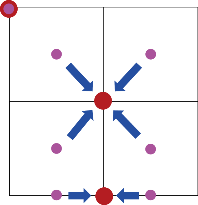
Restriction operation: four-point scheme for inner gird points, two-point scheme for boundary gird points and one-point scheme for corner gird points, pink points stand for fine grids, red points denote coarse grids and blue arrows represent the restriction operation
-
(2)
Prolongation operation
In the left half part of V-cycle (see Fig. 1), the correction of unknown pressure \({\varvec{e}}^{k}\) can be obtained on coarse mesh levels. Correspondingly, in the prolongation operation of the right half part of V-cycle, the correction \({\varvec{e}}^{k}\) is transferred form coarse mesh level k + 1 to fine mesh level k to obtain a better initial guess for unknown pressure. Similar to the restriction operator, the prolongation operator is dependent on the discrete scheme of pressure equation. In this study, the four-point scheme, two-point scheme and one-point scheme prolongation operators are, respectively, adopted for the prolongation of inner, boundary and corner grid points, as shown in Fig. 3. Commonly, the prolongation operator can be set as the transpose of restriction operator. It should be pointed out that the discrete coefficients and source term on coarse mesh levels have been calculated in the left half part of V-cycle; thus, there is no necessary to prolongate the discrete coefficients and source term from coarse mesh levels to fine mesh levels.
Fig. 3 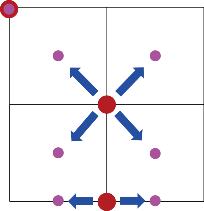
Prolongation operation: four-point scheme for inner gird points, two-point scheme for boundary gird points and one-point scheme for corner gird points, pink points stand for fine grids, red points denote coarse grids and blue arrows represent the prolongation operation
-
(3)
Smooth operation
In smooth operations, the algebraic pressure equation (12) can be solved by using different solvers, such as Jacobi iteration, Gauss–Seidel iteration, successive over-relaxation and conjugate gradient. Commonly, the smooth in the left half part of V-cycle is called pre-smooth and that in the right half part of V-cycle is called post-smooth. In this work, the Gauss–Seidel iteration is applied to both the pre-smooth and post-smooth operations. It should be noted that to save computational cost, the PR-EOS is not solved on coarse mesh levels in our FAS multigrid method. The compressibility factor Z on coarse mesh level is obtained by restricting Z from its neighboring fine mesh level. Although the numerical accuracy of unknown pressure on coarse mesh levels may be reduced slightly, it does not exert effects on the prediction accuracy of pressure on the finest mesh level.
To show the FAS multigrid method for solving the compressible flow equation more clearly, the pseudo-code (Briggs et al. 2000) is presented in Table 1. It can be clearly seen that compared with the POD–Galerkin model which is established in reduced-order subspace to accelerate the simulation of compressible flow (Wang et al. 2017a, b, Wang et al. 2018; Li et al. 2020a), the multigrid method solves Eq. (12) in the full-order space (the finest mesh level) with fixed dimension n. The purpose of computations on coarse mesh levels is just to obtain the correction of unknown pressures.
Table 1 FAS multigrid algorithm for solving the compressible flow equation


3.3 DEIM reduced-order model for Peng–Robinson equation of state
In traditional solution of EOS, the algebraic method for finding the roots of cubic equation is usually applied to solve the PR-EOS (7), which is extremely computational cost. Actually, it is not difficult to understand the heavy computational burden for solving PR-EOS; here, we explain this issue in detail. In algebra, the cubic polynomial PR-EOS (7) is a function of compressibility factor,
where a is nonzero.
Setting \(f(Z) = 0\) produces a cubic equation of the form,
It is known that if all of the coefficients a, b, c and d of the cubic equation are real numbers, then Eq. (14) has at least one real root due to the fundamental theorem of algebra. And all of the roots of Eq. (14) can be found algebraically according to the Abel–Ruffini theorem, but this process is always time-consuming. Furthermore, the cubic equation should be solved on all grid points in the computational domain with dimension n, which will lead to heavy computational burden in the simulation.
To accelerate the solution of PR-EOS (7), in this study, a reduced-order model called discrete empirical interpolation method (DEIM) (Chaturantabut and Sorensen 2010) is used to determine few significant spatial grid points in the computational domain; then, the PR-EOS (7) is solved by cube root finding algorithm only on the selected grid points instead of on all grids points. To select appropriate interpolation points, here the compressibility factor is supposed as the function of interest,
The DEIM approximates \(f(Z)\) by projecting it onto a subspace that spanned by a projection basis of dimension \(m \ll n\) obtained through eigenvalue decomposition or singular value decomposition of \(f(Z)\) snapshots. The approximation from projecting \({\varvec{f}}\left( Z \right) = \left[ {f_{1} \left( Z \right), \cdot \cdot \cdot ,f_{n} \left( Z \right)} \right]\) onto the subspace spanned by the basis \(\left\{ {{\varvec{w}}_{1} , \cdot \cdot \cdot ,{\varvec{w}}_{m} } \right\} \subset {\mathbb{R}}^{n}\) is of the form,
where the projection basis \({\varvec{W}} = \left[ {{\varvec{w}}_{1} , \cdot \cdot \cdot ,{\varvec{w}}_{m} } \right] \subset {\mathbb{R}}^{n \times m}\) and \({\varvec{c}}\left( Z \right)\) is the corresponding vector of reduced-order coefficients.
To determine \({\varvec{c}}\left( Z \right)\), m distinguished rows are selected from the overdetermined system \({\varvec{f}}\left( Z \right) = {\varvec{Wc}}\left( Z \right)\) in DEIM,
where \({\varvec{e}}_{{\xi_{i} }} = \left[ {0, \cdot \cdot \cdot ,0,1,0, \cdot \cdot \cdot ,0} \right]^{\text{T}} \subset {\mathbb{R}}^{n}\) is the \(\xi_{i}\) th column of the identity matrix \({\varvec{I}}_{n} \subset {\mathbb{R}}^{n \times m}\) for \(i = 1, \cdot \cdot \cdot ,m\).
Suppose \({\varvec{S}}^{\text{T}} {\varvec{W}}\) is nonsingular, then the coefficient vector \({\varvec{c}}\left( Z \right)\) can be computed uniquely from,
Then, the final approximation of \({\varvec{f}}\left( Z \right)\) can be expressed as,
It can be clearly seen from Eq. (19) that the approximation of \({\varvec{f}}\left( Z \right)\) can be computed only on the selected m grid points \(\left\{ {\xi_{1} , \ldots ,\xi_{m} } \right\}\) in the subspace with the dimension is reduced from n to m. It means that the PR-EOS (7) can be solved efficiently only on selected interpolation points instead of on all gird points in the domain, which can improve the computational efficiency dramatically. It is worth noting that to obtain the final approximation of \({\varvec{f}}\left( Z \right)\), the projection basis \(\left\{ {{\varvec{w}}_{1} , \ldots ,{\varvec{w}}_{m} } \right\}\) and interpolation grid points \(\left\{ {\xi_{1} , \ldots ,\xi_{m} } \right\}\) must be precomputed and specified: (1) for the determination of projection basis, it is constructed by applying the singular value decomposition or eigenvalue decomposition on snapshots of \({\varvec{f}}\left( Z \right)\) obtained from the original full-order space under various calculation conditions. The quality of snapshots \({\varvec{f}}\left( Z \right)\) can affect the prediction accuracy of DEIM obviously. Then, the DEIM approximation can be uniquely determined by the projection basis. Note that this projection basis not only specifies the projection subspace used in the approximation, but also determines the interpolation points used for computing the discrete coefficients of the approximation; (2) for the determination of interpolation points, they are selected inductively from the projection basis \(\left\{ {{\varvec{w}}_{1} , \ldots ,{\varvec{w}}_{m} } \right\}\) according to the DEIM algorithm, readers of interest can refer to (Chaturantabut and Sorensen 2010) for more technique details.
In summary, it can be seen that the DEIM approach approximates the function \({\varvec{f}}\left( Z \right)\) by combining projection with interpolation. It constructs specially selected interpolation points that specify an interpolation-based projection to provide a nearly L2 optimal subspace approximation to \({\varvec{f}}\left( Z \right)\) with low computational cost. Equation (19) indicates that a certain coefficient matrix (projection basis W and interpolation points S) can be precomputed, and as a result, the complexity in evaluating \({\varvec{f}}\left( Z \right)\) becomes proportional to the number of selected interpolation points.
4 Results and discussion
In this section, numerical performances (accuracy and acceleration) of multigrid-DEIM semi-reduced-order model are evaluated by a single-phase compressible flow (described by the model problem in Sect. 2) in two-dimensional porous media. The numerical simulation is performed using an in-house code on an Intel Xeon E5-2640, CPU2.60 GHz PC with 64.00 GB of RAM.
4.1 Case description
Figure 4 shows a 100 m × 100 m porous media domain. The west and east boundaries of this domain are set as pressure boundaries pw and pe, and both the north and south boundaries are set as Newman boundaries with zero velocity. The porosity of this domain is set as 0.2, the red region stands for a large permeability value 100 mD and the five blue regions represent a small permeability value 1 mD, respectively. In this study, 100 × 100 uniform grids are utilized to discretize the domain, and the grid index in x–y Cartesian coordinate is (i, j) with 0 ≤ i, j ≤ 101 (including boundary girds). Other calculation parameters used in the simulation are shown in Table 2. Note that the influence of temperature variation is ignored thus the compressible flow is an isothermal flow, and only methane is considered and a projection well is located at the right-top of the domain (grid index is (100, 100)) with a production rate qm = 0.01 kg/(m3·s).

Permeability distribution in the porous media domain
In multigrid-DEIM semi-reduced-order model, first the projection basis should be precomputed, this step is called offline computation that is carried out only one time in simulation (the computational cost can be ignored). To validate the correctness of multigrid-DEIM semi-reduced-order model and evaluate its online prediction ability, four groups of pressure boundary values are applied to obtain the projection basis at offline computation stage and one group of pressure boundary values is used to evaluate the prediction ability and numerical performance at online prediction stage, as shown in Table 2. At offline computation stage, 500 snapshots of the function \({\varvec{f}}\left( Z \right)\) [Eq. (15)] are considered in each group; thus, a total of 2000 snapshots are used to extract the projection basis. Commonly, the eigenvalue decomposition or singular value decomposition can be applied to compute the projection basis, readers of interest can refer to (Li et al. 2019a) for more details. Note that the quality of projection basis has significant effects on the prediction accuracy of DEIM, a good projection basis is capable to recover the information of original full-order problem as much as possible. Therefore, snapshots of function \({\varvec{f}}\left( Z \right)\) should be chosen carefully in order to obtain a good projection basis.
4.2 Selection of DEIM interpolation points
In multigrid-DEIM semi-reduced-order model, the adopted FAS multigrid method is a full-order model solver; the parameter settings of FAS multigrid method only affect the acceleration but not the computational accuracy. In this study, three mesh levels are applied in FAS multigrid method, both the pre-smooth and post-smooth numbers are set as 3, and the Gauss–Seidel iteration is used as the smoother. Different from FAS multigrid method, the DEIM for the solution of PR-EOS is a reduced-order model, the projection basis and interpolation points can influence both the acceleration and prediction accuracy substantially. When projection basis is determined, the prediction accuracy of DEIM is dependent on interpolation points. To guarantee good prediction accuracy, the interpolation points should be selected carefully in order to achieve a balance between the acceleration and accuracy.
For convenience, in this study, 5, 10, 15 and 20 DEIM interpolation points are, respectively, tested to determine an optimal number of interpolation points. According to DEIM algorithm (Chaturantabut and Sorensen 2010), the four sets of selected interpolation points are determined and shown in Fig. 5, and the corresponding grid index of these points is presented in Table 3. It can be found that most of selected interpolation points are located at where the permeability changes sharply, indicating that the interpolation points are selected to capture the variation of function \({\varvec{f}}\left( Z \right)\) (quantity of interest).

Distribution of selected DEIM interpolation points
To select an appropriate number of interpolation points, the online simulation is performed in which the above four sets of interpolations points are, respectively, tested. The average relative errors between the results predicted by multigrid-DEIM semi-reduced-order model and that calculated by standard semi-implicit method are displayed in Fig. 6. Note that the studied model problem is an unsteady flow; thus, average relative errors of pressure, Darcy velocity and compressibility factor at four different simulation times (t1 = 5000△t, t2 = 50,000△t, t3 = 100,000△t, t4 = 150,000△t) are presented. From Fig. 6, it can be clearly seen that the average relative errors of the above four variables decline with the increase in interpolation point number, indicating that more interpolation points can recover more information of the original full-order problem and then the numerical results with high numerical accuracy can be obtained. However, it can also be found that the average relative errors of these four variables almost have no change when more than 10 interpolation points are selected. It indicates that 10 interpolation points are already enough for online prediction with satisfactory accuracy in this study, extra interpolation points contribute a little to the prediction accuracy.

Average relative errors between the results of multigrid-DEIM and that of standard semi-implicit method with different numbers of interpolation points
Figure 7 shows the acceleration of multigrid-DEIM semi-reduced-order model compared with the standard semi-implicit method under same calculation conditions. It can be clearly observed that with the increase in interpolation points, the speedup of multigrid-DEIM semi-reduced-order model declines almost linearly at the four different simulation times, and the speedup is approximately a monotonic linear function of the number of interpolation points. Based on the above analysis of Figs. 6 and 7, it is reasonable to select 10 interpolation points to achieve acceleration and preserve good prediction accuracy at the same time in this work.

Acceleration of multigrid-DEIM semi-reduced-order model
4.3 Discussion of prediction results
In this part, the numerical accuracy and acceleration of multigrid-DEIM semi-reduced-order model are compared with that of standard semi-implicit method at the online prediction stage. It should be mentioned that from Fig. 6 it can be seen the average relative errors change slightly at the simulation times t2, t3 and t4; thus, in the following text, only the results at the simulation times t1 and t3 are illustrated. Figures 8, 9, 10 and 11, respectively, show the pressure, Darcy velocity and compressibility factor obtained by using the multigrid-DEIM semi-reduced-order model at t1 and t3. To evaluate the prediction accuracy, simulation results of standard semi-implicit method are also presented in the same figure for qualitative comparison.

Comparison of pressure obtained by multigrid-DEIM semi-reduced-order model (red dashed line) and that calculated by standard semi-implicit method (blue line)

Comparison of u-velocity obtained by multigrid-DEIM semi-reduced-order model (red dashed line) and that calculated by standard semi-implicit method (blue line)

Comparison of v-velocity obtained by multigrid-DEIM semi-reduced-order model (red dashed line) and that calculated by standard semi-implicit method (blue line)

Comparison of compressibility factor obtained by multigrid-DEIM semi-reduced-order model (red dashed line) and that calculated by standard semi-implicit method (blue line)
From the comparison presented in Figs. 8, 9, 10 and 11, it can be clearly seen that the red dashed line representing the results of multigrid-DEIM semi-reduced-order model agree well with the blue line denoting the results of standard semi-implicit method at simulation times t1 and t3. In specific, the pressure, Darcy velocity and compressibility factors predicted by our proposed multigrid-DEIM semi-reduced-order model have almost the same numerical accuracy with the standard semi-implicit method. Only the u and v Darcy velocities show slight distinctions between these two methods at simulation time t1. It is not difficult to understand the relative large error of Darcy velocity compared with pressure. According to the Darcy’s law, the Darcy velocity depends on the pressure gradient and hydraulic conductivity, the error of pressure may be enlarged in the computation of Darcy velocity. Overall, Figs. 8, 9, 10 and 11 can qualitatively demonstrate that the proposed multigrid-DEIM semi-reduced-order model possesses good prediction accuracy with a slight accuracy loss.
To quantitatively evaluate the numerical accuracy of multigrid-DEIM semi-reduced-order model, the average relative errors of pressure, Darcy velocity and compressibility factor obtained at simulation times t1–t4 are presented in Table 4. It can be seen that except for the error of v Darcy velocity at simulation time t1, the average relative errors of remaining variables are small enough to neglect. For example, at the simulation times t2–t4 the average relative error of pressure has the order of magnitude 10−7%, and that of Darcy velocity and compressibility factor have the order of magnitude 10−6% and 10−4%, respectively. One main reason for the large error of Darcy velocity at simulation time t1 is that the flow at t1 is still not fully developed and in unsteady state, the variation of Darcy velocity is relatively large. When the flow is well developed and in steady state, the Darcy velocity will change slightly and the average relative error will be reduced. Overall, it can be referred from Table 4 that the results calculated by multigrid-DEIM semi-reduced-order model match well with the simulation results of standard semi-implicit method, the average relative errors between these two methods are negligible for engineering applications. Thus, it can be proved that the multigrid-DEIM semi-reduced-order model is capable to predict the numerical results with tiny accuracy loss.
To evaluate the acceleration of multigrid-DEIM semi-reduced-order model, the CPU time consumption and corresponding speedup of the above cases are presented in Table 5. It can be clearly seen that the computation of proposed multigrid-DEIM semi-reduced-order model is faster than the standard semi-implicit methods at the four simulation times t1–t4. For example, at simulation times t1 and t2, the multigrid-DEIM semi-reduced-order model can achieve 65.33 and 64.21 times of acceleration compared with the standard semi-implicit method. Overall, the speedup of multigrid-DEIM semi-reduced-order model is approximately two orders of magnitude, which is very attractive for engineering applications. In summary, Figs. 8, 9, 10 and 11 and Tables 4 and 5 demonstrate that the proposed multigrid-DEIM semi-reduced-order model enjoys a very attractive computational efficiency (two orders of magnitude faster) while preserving the similar accuracy of the standard semi-implicit method.
5 Conclusions
An efficient multigrid-DEIM semi-reduced-order model is proposed in this study for fast simulation of unsteady single-phase compressible flow through porous media. In the framework of multigrid-DEIM semi-reduced-order model, the FAS multigrid method is applied to accelerate the solution of flow equation in original full-order space, and at the same time, the DEIM is used to speed up the solution of PR-EOS in a reduced-order subspace with only few selected interpolation points. The studied model problem is introduced briefly and the establishment of multigrid-DEIM semi-reduced-order model is illustrated step by step. To evaluate the numerical performances of multigrid-DEIM semi-reduced-order model, an unsteady single-phase compressible flow in two-dimensional porous media is simulated carefully and following concluding remarks can be summarized:
-
(1)
The interpolation points have significant effect on the prediction accuracy of compressibility factor and the whole computational acceleration. The selection of interpolation points should be carried out carefully to obtain appreciable acceleration at the same time preserve good prediction accuracy. In this study, 10 spatial grid points are selected based on the elaborate evaluation of four sets of interpolation points, with the dimension reduced from 10,000 to order 10 in the solution of PR-EOS.
-
(2)
Compared with the traditional semi-implicit method, the multigrid-DEIM semi-reduced-order model is capable to predict the numerical results accurately, and the average relative errors of pressure, Darcy velocity and compressibility factor only have the order of magnitude 10−7%, 10−6%, 10−4%, which are negligible in real engineering applications. At the same time, the acceleration of multigrid-DEIM semi-reduced-order model at different simulation times can up to approximate two orders of magnitude for two-dimensional simulations.
In addition, it should be noted that the proposed multigrid-DEIM semi-reduced-order model is a general framework, it is straightforward to extend this model to different problem conditions (for instance, three-dimensional domain and different production rates), and further computational gains can be achieved if other techniques are coupled, such as the parallel computing. In the future work, the possible research directions can focus on the application of presented model to the multiphase flow and multi-component flow in porous media.
References
Akhmetzyanov AA, Ermolaev AI, Grebennik OS. Parallel computing in optimal design of development of multilayer oil and gas fields. IFAC Proc Vol. 2012;45(8):151–6. https://doi.org/10.3182/20120531-2-NO-4020.00028.
Akkutlu IY, Efendiev Y, Vasilyeva M. Multiscale model reduction for shale gas transport in fractured media. Comput Geosci. 2016;20(5):953–73. https://doi.org/10.1007/s10596-016-9571-6.
Akkutlu IY, Efendiev Y, Vasilyeva M, Wang Y. Multiscale model reduction for shale gas transport in a coupled discrete fracture and dual-continuum porous media. J Nat Gas Sci Eng. 2017;48:65–76. https://doi.org/10.1016/j.jngse.2017.02.040.
Akkutlu IY, Efendiev Y, Vasilyeva M, Wang Y. Multiscale model reduction for shale gas transport in poroelastic fractured media. J Comput Phys. 2018;353:356–76. https://doi.org/10.1016/j.jcp.2017.10.023.
Alzahabi A, Berlow N, Soliman M, Alqahtani G. Multigrid fracture stimulated reservoir volume mapping coupled with a novel mathematical optimization approach to shale reservoir well and fracture design. J Sust Energy Eng. 2016;4(3–4):310–34. https://doi.org/10.7569/JSEE.2016.629521.
Amini S, Mohaghegh S. Application of machine learning and artificial intelligence in proxy modeling for fluid flow in porous media. Fluids. 2019;4(3):126. https://doi.org/10.3390/fluids4030126.
Birgle N, Masson R, Trenty L. A domain decomposition method to couple nonisothermal compositional gas liquid Darcy and free gas flows. J Comput Phys. 2018;368:210–35.
Briggs WL, Henson VE, McCormick SF. A multigrid tutorial. 2nd ed. Philadelphia: SIAM; 2000.
BP Energy Outlook. 2019 edition. London, United Kingdom, 2019
Cao P, Liu J, Leong YK. A fully coupled multiscale shale deformation-gas transport model for the evaluation of shale gas extraction. Fuel. 2016;178:103–17. https://doi.org/10.1016/j.fuel.2016.03.055.
Chaturantabut S, Sorensen DC. Nonlinear model reduction via discrete empirical interpolation. SIAM J Sci Comput. 2010;32(5):2737–64. https://doi.org/10.1137/090766498.
Cheung SW, Chung ET, Efendiev Y, Gildin E, Wang Y, Zhang J. Deep global model reduction learning in porous media flow simulation. Comput Geosci. 2020;24(1):261–74. https://doi.org/10.1007/s10596-019-09918-4.
Fung LS, Du S. Parallel-simulator framework for multipermeability modeling with discrete fractures for unconventional and tight gas reservoirs. SPE J. 2016;21(4):1370–85. https://doi.org/10.2118/179728-PA.
Ghasemi M, Gildin E. Model order reduction in porous media flow simulation using quadratic bi- linear formulation. Comput Geosci. 2016;20(3):723–35. https://doi.org/10.1007/s10596-015-9529-0.
Gries S, Stüben K, Brown GL, Chen D, Collins DA. Preconditioning for efficiently applying algebraic multigrid in fully implicit reservoir simulations. SPE J. 2014;19(4):726–36. https://doi.org/10.2118/163608-PA.
Ho MT, Zhu L, Wu L, Wang P, Guo Z, Li ZH, Zhang Y. A multi-level parallel solver for rarefied gas flows in porous media. Comput Phys Commun. 2019;234:14–25. https://doi.org/10.1016/j.cpc.2018.08.009.
Holderbaum T, Gmehling J. PSRK: a group contribution equation of state based on UNIFAC. Fluid Phase Equilib. 1991;70(2–3):251–65. https://doi.org/10.1016/0378-3812(91)85038-V.
Jambunathan R, Levin DA. Advanced parallelization strategies using hybrid MPI-CUDA octree DSMC method for modeling flow through porous media. Comput Fluids. 2017;149:70–87. https://doi.org/10.1016/j.compfluid.2017.02.020.
Kani JN, Elsheikh AH. Reduced-order modeling of subsurface multi-phase flow models using deep residual recurrent neural networks. Transp Porous Media. 2019;126(3):713–41. https://doi.org/10.1007/s11242-018-1170-7.
Kontogeorgis GM, Voutsas EC, Yakoumis IV, Tassios DP. An equation of state for associating fluids. Ind Eng Chem Res. 1996;35(11):4310–8. https://doi.org/10.1021/ie9600203.
la Cour Christensen M, Eskildsen KL, Engsig-Karup AP, Wakefield M. Nonlinear multigrid for reservoir simulation. SPE J. 2016;21(3):888–98. https://doi.org/10.2118/178428-PA.
Li J, Yu B, Zhao Y, Wang Y, Li W. Flux conservation principle on construction of residual restriction operators for multigrid method. Int Commun Heat Mass Transf. 2014;54:60–6. https://doi.org/10.1016/j.icheatmasstransfer.2014.03.013.
Li J, Zhang T, Sun S, Yu B. Numerical investigation of the POD reduced-order model for fast predictions of two-phase flows in porous media. Int J Numer Meth Heat Fluid Flow. 2019a;29(11):4167–204. https://doi.org/10.1108/HFF-02-2019-0129.
Li J, Fan X, Wang Y, Yu B, Sun S, Sun D. A POD-DEIM reduced model for compressible gas reservoir flow based on the Peng-Robinson equation of state. J Nat Gas Sci Eng. 2020a;79:103367. https://doi.org/10.1016/j.jngse.2020.103367.
Li Y, Zhang T, Sun S, Gao X. Accelerating flash calculation through deep learning methods. J Comput Phys. 2019b;394:153–65. https://doi.org/10.1016/j.jcp.2019.05.028.
Li Z, Qi Z, Yan W, Xiang Z, Ao X, Huang X, Mo F. Prediction of production performance of refractured shale gas well considering coupled multiscale gas flow and geomechanics. Geofluids. 2020b;2020:9160346. https://doi.org/10.1155/2020/916034.
Lovett S, Nikiforakis N, Monmont F. Adaptive mesh refinement for compressible thermal flow in porous media. J Comput Phys. 2015;280:21–36. https://doi.org/10.1016/j.jcp.2014.09.017.
Peng DY, Robinson DB. A new two-constant equation of state. Ind Eng Chem Fundam. 1976;15(1):59–64. https://doi.org/10.1021/i160057a011.
Popov V, Power H. DRM-MD approach for the numerical solution of gas flow in porous media, with application to landfill. Eng Anal Bound Elem. 1999;23(2):175–88. https://doi.org/10.1016/S0955-7997(98)00054-X.
Schrefler BA, Wang X, Salomoni VA, Zuccolo G. An efficient parallel algorithm for three-dimensional analysis of subsidence above gas reservoirs. Int J Numer Meth Fluids. 1999;31(1):247–60. https://doi.org/10.1002/(SICI)1097-0363(19990915)31:1%3c247:AID-FLD966%3e3.0.CO;2-D.
Skogestad JO, Keilegavlen E, Nordbotten JM. Domain decomposition strategies for nonlinear flow problems in porous media. J Comput Phys. 2013;234:439–51. https://doi.org/10.1016/j.jcp.2012.10.001.
Soave G. Equilibrium constants from a modified Redlich-Kwong equation of state. Chem Eng Sci. 1972;27(6):1197–203. https://doi.org/10.1016/0009-2509(72)80096-4.
Stavroulakis GM, Papadrakakis M. Advances on the domain decomposition solution of large scale porous media problems. Comput Methods Appl Mech Eng. 2009;198(21–26):1935–45. https://doi.org/10.1016/j.cma.2009.01.003.
Tan X, Gildin E, Florez H, Trehan S, Yang Y, Hoda N. Trajectory-based DEIM (TDEIM) model reduction applied to reservoir simulation. Comput Geosci. 2019;23(1):35–53. https://doi.org/10.1007/s10596-018-9782-0.
Tanaka S, Wang Z, Dehghani K, He J, Velusamy B, Wen X H. Large scale field development optimization using high performance parallel simulation and cloud computing technology. In: SPE Annual Technical Conference and Exhibition, 24–26 September, Dallas, Texas, USA; 2018. https://doi.org/10.2118/191728-MS.
van der Waals J D – Nobel Lecture. NobelPrize.org. Nobel Media AB 2020. Wed. 26 Aug 2020. https://www.nobelprize.org/prizes/physics/1910/waals/lecture/
Wang L, Osei-Kuffuor D, Falgout R, Mishev I, Li J. Multigrid reduction for coupled flow problems with application to reservoir simulation. In: SPE Reservoir Simulation Conference, 20-22 February, Montgomery, Texas, USA; 2017. https://doi.org/10.2118/182723-MS.
Wang S, Feng Q, Javadpour F, Zha M, Cui R. Multiscale modeling of gas transport in shale matrix: an integrated study of molecular dynamics and rigid-pore-network model. SPE J. 2020;25:1–27. https://doi.org/10.2118/187286-PA.
Wang Y, Sun S, Yu B. Acceleration of gas flow simulations in dual-continuum porous media based on the mass-conservation POD method. Energies. 2017;10(9):1380. https://doi.org/10.3390/en10091380.
Wang Y, Yu B, Wang Y. Acceleration of gas reservoir simulation using proper orthogonal decomposition. Geofluids. 2018;2018:8482352. https://doi.org/10.1155/2018/8482352.
Yang Y, Ghasemi M, Gildin E, Efendiev Y, Calo V. Fast multiscale reservoir simulations with POD-DEIM model reduction. SPE J. 2016;21(6):1–14. https://doi.org/10.2118/173271-PA.
Yang Y, Gildin E, Efendiev Y, Calo V (2017) Online adaptive POD-DEIM model reduction for fast simulation of flows in heterogeneous media. In: SPE Reservoir Simulation Conference, 20–22 February, Montgomery, Texas, USA; 2017. https://doi.org/10.2118/182682-MS
Yu H, Fan J, Xia J, Liu H, Wu H. Multiscale gas transport behavior in heterogeneous shale matrix consisting of organic and inorganic nanopores. J Nat Gas Sci Eng. 2020;75:103139. https://doi.org/10.1016/j.jngse.2019.103139.
Acknowledgements
This study is supported by the National Natural Science Foundation of China (Nos. 51904031, 51936001), the Beijing Natural Science Foundation (No. 3204038) and the Jointly Projects of Beijing Natural Science Foundation and Beijing Municipal Education Commission (No. KZ201810017023).
Author information
Authors and Affiliations
Corresponding author
Ethics declarations
Conflict of interest
The authors declare that they have no conflict of interest.
Additional information
Edited by Xiu-Qiu Peng
Rights and permissions
Open Access This article is licensed under a Creative Commons Attribution 4.0 International License, which permits use, sharing, adaptation, distribution and reproduction in any medium or format, as long as you give appropriate credit to the original author(s) and the source, provide a link to the Creative Commons licence, and indicate if changes were made. The images or other third party material in this article are included in the article's Creative Commons licence, unless indicated otherwise in a credit line to the material. If material is not included in the article's Creative Commons licence and your intended use is not permitted by statutory regulation or exceeds the permitted use, you will need to obtain permission directly from the copyright holder. To view a copy of this licence, visit http://creativecommons.org/licenses/by/4.0/.
About this article

Cite this article
Li, JF., Yu, B., Wang, DB. et al. An efficient multigrid-DEIM semi-reduced-order model for simulation of single-phase compressible flow in porous media. Pet. Sci. 18, 923–938 (2021). https://doi.org/10.1007/s12182-020-00509-y
Received:
Published:
Issue Date:
DOI: https://doi.org/10.1007/s12182-020-00509-y