Habitat Suitability Curves for Freshwater Macroinvertebrates of Tropical Andean Rivers

Abstract

Sustainable river management requires a thorough understanding of the response of aquatic biota to riverine microhabitat variability. The purpose of this study was to assess macroinvertebrate hydraulic-habitat suitability in Ecuadorian Andean rivers to support habitat modelling for sustainable ecosystem management. 597 macroinvertebrate samples were collected from ten sampling stations the Yanuncay River, Ecuador. Physical, chemical, hydraulic and habitat variables were measured/calculated. Froude number, Reynolds number, substrate index and algae coverage were major drivers of macroinvertebrate response, and were used to develop suitability curves for Baetodes, Andesiops, Camelobaetidius, Ecuaphlebia, Anacroneuria, Atopsyche, Simulium and Palpomyia using General Additive Models. Standardised density contours of taxa as functions of hydraulic and habitat variables were also developed. Taxonomic response was related to body structures/shapes and feeding habits. Baetodoes, Simulium, Anacroneuria and Atopsyche preferred fast flowing waters, and thus, they could be significantly affected in case of flow reduction. Similar habitat suitability curves were developed from the main river and the tributaries, possibly due to the short distance between the sampling stations. This study fills a major knowledge gap by developing macroinvertebrate habitat suitability curves for future physical habitat simulations and environmental flow assessments in the Andean region.

1. Introduction

In river ecosystems, environmental and biological factors act at multiple spatial and temporal scales, influencing the distribution patterns of aquatic biodiversity. In this regard, most studies on aquatic macroinvertebrates focus on large spatial and temporal scales [1,2,3], and only few on smaller scales [4,5]. Ecological or hydrological processes acting at larger scales shape smaller-scale habitats, resulting in a nested hierarchy of interconnected habitats where species become more and more specialised as habitat conditions become site-specific [6]. Moreover, aquatic communities in lotic ecosystems have irregular spatial distribution patterns [7] due to specific physical, hydrological and/or hydraulic conditions [4,8] that shape aquatic biota through adaptation processes resulting in highly specialised species [9]. Hence, the main hydraulic (flow velocity and water depth) and habitat (substrate type) characteristics and their combined influence have been assessed as major drivers of the spatial distribution of benthic communities at the microhabitat scale [10].

Most studies on the response of macroinvertebrates to hydraulic-habitat variability have been carried out in temperate zones, indicating that primary hydraulic and habitat drivers of biotic distribution are flow velocity [11,12,13], water depth [11,12,13], Froude number [13,14], Reynolds number [15], substrate type [14] and shear stress [14]. These eco-hydraulic studies have generated basic knowledge for the development of habitat models, incorporating various discharge scenarios that reflect different levels of anthropogenic impact [16,17]. However, in tropical zones, knowledge on the hydraulic response of aquatic macroinvertebrates remains limited [18,19,20].

While in other latitudes aquatic species are used to holistically assess the effect of natural or anthropic impacts on the ecological status of rivers [21,22], in Ecuador and other Andean countries, legislation on environmental flows is established mainly on empirical hydrological methods [23,24], without considering the influence of physical or hydraulic variability on aquatic biota. Moreover, in this region the alteration of aquatic and terrestrial habitats is increasing due to the construction of dams or water reservoirs of various sizes [25,26], which is likely to cause a disconnection of habitats, impacting in this way the aquatic communities [25].

Several methods have been applied to study the responses of aquatic invertebrates to physical and hydraulic-habitat variables. The biological response to hydraulic variability has been investigated by using techniques such as adjustment of polynomials [27], exponential polynomial functions [11] or local polynomial regression [28]. Other multivariate methods received greater attention in recent years such as the Generalised Additive Models (GAMs) [16,29,30]. Some other studies used large amounts of data with Boosted Regression Trees, Random Forests [28] and fuzzy-logic-based models [28,30]. GAMs are considered an appropriate method for estimating the habitat suitability of aquatic species [31] including macroinvertebrates [16,29,30] because it enables overcoming inherent pitfalls of other more traditional methods that do not assess uncertainty and do not consider interactions among hydraulic-habitat variables [16]. Also, GAMs are appropriate for developing non-linear and non-monotonic habitat suitability curves between the response and predictor variables [31]. These curves can be further included in eco-hydraulic models such as the System for Environmental Flow Analysis (SEFA) [32] or the River Hydraulic Habitat Simulation (RHYHABSIM) [33] for physical habitat modelling purposes, aiming at assessing the instream flow requirements of macroinvertebrates to maintain life-supporting freshwater capacity and native biodiversity.

Suitability curves are expensive to elaborate, and this restricts their use for carrying out individual instream flow assessments [16]. As an acceptable cost-effective practice, suitability curves developed in large rivers are normally transferred to other river types. However, assuming similar habitat suitability of aquatic organisms in different rivers might not be correct since their response to habitat variability can vary importantly in space and time based on river size and flow variation [34,35,36]. In Ecuador, hydraulic-habitat suitability curves for macroinvertebrates do not exist; as such, this study is a pioneering effort to develop habitat suitability curves for macroinvertebrates in larger and smaller rivers.

Mitigation of flow regime alteration caused by human activities and application of stream management measures require the use of predictive models to quantify the environmental flow regimes to maintain biotic and abiotic processes within river systems [27]. However, prior to the application of such predictive models, scientific knowledge of the response of aquatic organisms to hydraulic and habitat variability is necessary [37].

The purpose of this study was to assess the response of macroinvertebrates to microhabitats characterised by certain hydraulic and habitat conditions and to develop suitability curves for future physical habitat modelling in the high Andean rivers of southern Ecuador. The specific objectives were to: (a) identify the major hydraulic and habitat variables to develop habitat suitability curves; (b) develop habitat suitability curves for the most representative macroinvertebrate taxa in the Yanuncay main river and its tributaries; (c) compare the habitat suitability curves from the main river and its tributaries; and (d) produce contour curves of (standardised) density of the most representative macroinvertebrate taxa as a function of the most influential hydraulic and habitat variables. To the best of our knowledge, this is the first attempt to develop habitat suitability curves for dominant macroinvertebrate taxa in tropical Andean lotic ecosystems.

2. Materials and Methods

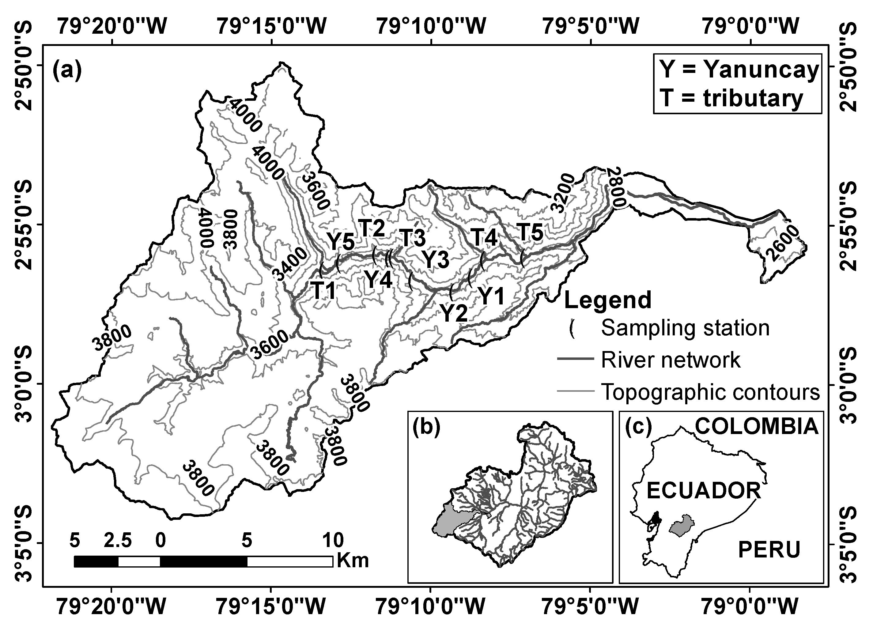
2.1. Study Area

Andean streams are characterised by highly variable discharge with sudden peak flows, highly variable topography and only two seasons, wet and drier, whose temporal bounds may vary drastically from year to year, and with respect to the average pattern [38,39]. Henceforth, particularly this seasonality is a clear distinctive difference between tropical (Andean) and temperate mountain streams, upon which there are also distinctive characteristics in terms of biotic communities. The study area is the sub-basin of the Yanuncay river (Figure 1a), which belongs to the Paute basin (Figure 1b). The Paute basin is one of the most important basins for the domestic and industrial development of Ecuador (Figure 1c) given that approximately 40% of the nation-wide consumed electricity is hydraulically generated in it [40]. The studied sub-basin has an area of about 418.9 km²; its elevation varies between 2520 and 4080 m above the sea level (a.s.l.). The slope is significantly irregular with valleys formed by steep transversal slopes. Above 3000 m a.s.l., the sub-basin presents a dominant (i.e., 90%) grass land termed as “Pajonal” (Calamagrostis sp.) [41], a typical vegetation cover of these Andean highlands (termed as “Páramo”), as well as some Quinua (Polylepis sp.) patches (i.e., 0.78%; [42]). The central sub-basin presents evergreen high montane forest patches with land dedicated to agricultural activities and cattle raising. In the lower parts significant human settlements occur. As in most of the Paute river basin, given the particular presence of the Andean mountain range, the climate of the Yanuncay sub-basin is affected by the winds of both, the Atlantic Ocean in the east and the Pacific Ocean in the west. Upon the analysis of rainfall data in the period 1997–2018, two main rainy seasons can be distinguished (i.e., January–May and October–December) with a single three-month drier season, i.e., July–September, although with the presence of rainfall, which matches prior research conclusions [38].

2.2. Abiotic Monitoring

Aiming at inspecting the eco-hydraulic dynamics of the studied taxa as a function of channel type, tributary and main river channels were considered separately, as well as a “global” (i.e., simultaneous) consideration of both channel types.

Ten sampling stations (five in the main river channel and five in the tributaries), surrounded by the same riverine forest, were established in the Yanuncay sub-basin (Figure 1a). The main river stations are distributed between 2919 (Y1) and 3194 (Y5) m a.s.l. Their substratum is dominated by boulder (>256 mm) and cobble (256–64 mm), and their longitudinal slope varies between 1.0% and 2.8%. The tributary stations are distributed between 2828 (T5) and 3236 (T1) m of elevation. Their substratum is dominated by boulders, cobbles and pebbles (64–4 mm) and their longitudinal slope varies between 0.25% and 6.50%.

For the 10 sampling stations, both biotic and abiotic measurements were performed in the two sampling campaigns (i.e., C1 on November 2017, average rainy period; and C2 on July 2018, average drier period). No sampling took place in periods of high peak flows owing to safety constraints and because macroinvertebrate communities are washed away during flooding. A 200 m reach segment was chosen for the monitoring of each sampling station. The choice of the segment was based on accessibility for monitoring purposes and on the representativeness of all of the mesohabitats of the study site.

Hydraulic measurements were carried out at every biotic sampling point considering a microhabitat scale; 300 at the main river and 297 at the tributaries. Water depth (m) was determined using a graduated rod; water velocity (m s⁻¹) was measured with a propeller-type flow-meter (Hydromate CMC3, Hydrological Services Pty. Ltd., Sidney, Australia). The stream discharge was estimated at each sampling station and occasion by employing the velocity integration method [43]. In addition, the proportions of substrate types at each sampling point (considering the Surber net area: 900 cm²) were determined using this simplified classification: boulder (>256 mm), coarse cobble (256–128 mm), fine cobble (128–64 mm), very coarse pebble (64–32 mm), coarse pebble (32–16 mm), medium pebble (16–8 mm), fine pebble (8–4 mm), granule gravel (4–2 mm), sand (2–0.06 mm), silt (0.06–0.004 mm), and clay (<0.004 mm), according to the guidelines provided by Blair and McPherson [44].

Physical-chemical variables were recorded in situ at every sampling station during each sampling campaign through the use of a multiple water quality sensor (U-50 series, Horiba, HORIBA Ltd., Kyoto, Japan), including, water temperature (°C), electric conductivity (μS cm⁻¹), total dissolved solids (g·L⁻¹), pH, turbidity (NTU), dissolved oxygen (mg·L⁻¹), oxygen saturation (%) and the redox potential (mV).

2.3. Biotic Monitoring

Thirty macroinvertebrate samples were collected from different mesohabitats using a Surber net (area: 900 cm²; mesh size: 250 microns). In sampling campaign C1, 30 samples were collected at 9 sampling stations while at sampling station T5 it was only possible to collect 27 samples during the rainy period when too high discharges occurred (i.e., 297 samples were collected). In campaign C2, 30 samples were collected at every one of the 10 sampling stations (i.e., 300 samples were collected). Hence, a total of 597 macroinvertebrate samples were taken in both campaigns, 300 at the main river and 297 at the tributaries. The coverage of algae (Algae, %) and bryophytes (Bryo, %) per sampling quadrant (900 cm²) were visually estimated (by the same person), previously to each macroinvertebrate sampling. Macroinvertebrate samples were fixed in the field with 4% formaldehyde solution. In laboratory, all of the organism were sorted out and identified to genus level using taxonomic keys [45]. Higher taxonomic divisions were used for organisms belonging to the non-insect class, the subfamilies of Chironomidae and undistinguishable larvae of the Xiphocentronidae family.

Once all of the macroinvertebrate organisms were removed from the sample, the remaining sediment was used to determine the organic matter content in the sediment, according to the procedure of Steinman et al. [46].

2.4. Data Processing

Rare macroinvertebrate taxonomic groups, characterised by a relative abundance lower than 0.01% [47], were discarded from the statistical analysis. Furthermore, using the absolute abundance of every taxon, the density metric (ind. m⁻²) was calculated. Density was further standardised because biological data were collected at different discharges and times. Standardisation was achieved by dividing density estimates by their arithmetic mean calculated for every sampling campaign (C1 and C2) and for each channel type (main river and tributary). Hence, four groups of “standardised by mean” density (δ) data were generated, resulting from the consideration of two sampling campaigns and two channel types.

Hydraulic measurements were processed to calculate some hydraulic variables of interest. Hence, the Froude number (Fr), the ratio between the inertial and gravitational forces, was calculated as a function of water velocity, gravity acceleration and the hydraulic depth [48]. Also the Reynolds number (Re), the ratio between inertial and viscous forces, was calculated as a function of water velocity, the hydraulic radius and the kinematic viscosity [49]. Re values lower than 500 were assumed to characterise laminar flows, whilst Re > 12,000 characterised turbulent flows and 500 ≤ Re ≤ 12,000 characterised transitional flows.

Moreover, the roughness Reynolds number, an empirical variable which relates the roughness and flow parameters at which transition occurs at the surface of the roughness element of a river bed [50] was calculated as a function of the mean water velocity in the column of water, the height of the surface roughness element and the kinematic viscosity [50,51]. Roughness Reynolds number was used in this study after [52] detecting that this empirical criterion was importantly related to the spatial variation of invertebrates. Since roughness Reynolds number describes the roughness of the near-bed flow environment, values lower than 5 were assumed to characterise hydraulically smooth flows, whilst roughness Reynolds number > 70 characterised hydraulically rough flows (i.e., in rivers with coarse bed material) and 5 ≤ roughness Reynolds number ≤ 70 characterised transitional flows [51,52].

The percent coverage of each substrate category were used to calculate the Shannon-Wiener substrate diversity (SuD, [53]). SuD indicates the heterogeneity of the substrate. Further, the substrate index (SI) was calculated summing weighted substrate percentages [54], as follows: (0.08) % bedrock + (0.07) % boulder + (0.06) % cobble + (0.05) % pebble + (0.04) % granule gravel + (0.03) % sand. Given the summation properties of its mathematical expression SI varies between 3 (for a 100% sand content) and 8 (for a 100% bedrock content) and may adopt any real value in that range of variation. Further, the larger SI, the larger the sampled substrate sizes are.

2.5. Statistical Analysis

Spearman’s correlation analysis was performed on the 21 hydraulic and habitat variables for the datasets of the main and tributary river reaches. Three variables in the case of the main reach (i.e., velocity measured at 60% of the water depth, the roughness Reynolds number and the boulder substrate material) and 2 variables in the case of tributaries (i.e., velocity measured at 60% of the water depth and the roughness Reynolds number), presenting a significant correlation (r > 0.80, p < 0.05) with other hydraulic/habitat variables of higher interest for this study, were discarded from the rest of the analysis. Further, Bryophytes coverage was also discarded since it was not present in the main river reach. The Detrended Correspondence Analysis (DCA) was applied for selecting the appropriate multivariate model that was used, in turn, for determining the hydraulic and habitat variables influencing macroinvertebrate communities at microhabitat scale. DCA, based on the length of gradient (<3), suggested the use of the linear response multivariate model (Redundancy Analysis, RDA; [55]). Two RDA multivariate models were constructed [56]; one for the main river and another one for tributaries. The multivariate (DCA and RDA) analyses were carried out using non-standardised taxa densities, which, previously, were transformed using the log (x + 1) expression and standardised by species [55]. Forward selection was employed to select the hydraulic and habitat variables that had influence on the macroinvertebrate communities. For a better visualization of the resulting plot, the number of taxa was restricted to the 15 that had a best fit in the RDA models. These statistical analyses were carried out with the help of the CANOCO software version 5.02 [57].

Development of Habitat Suitability Curves

All variables selected by the RDA were used as predictors in GAMs but only the results of four hydraulic and habitat variables (Fr, Re, SI, and Algae) are presented herein. They were selected on the basis of their significance in the RDA, their similar use in past research [15,16], and the more meaningful interpretation of the respective GAMs based habitat suitability curves. Eight taxa were selected as response variables in the GAMs analysis based on their high occurrence and dominance in the samples, their sensitivity to river water quality [58], their significance in the RDA and their meaningful response in the GAMs. The application of the GAMs was achieved through the use of the Habitat Selection program (version 3.0, Jowett Consulting Ltd., Pukekohe, New Zealand) with a natural logarithmic (ln) link function [16,59]. In this way, the general expression of a full model is as follows:

$$\ln \left(\mathrm{Y}\right)={\mathrm{C}}_0+{\mathrm{C}}_1.\left({\mathrm{X}}_1\right)+{\mathrm{s}}_1\left({\mathrm{X}}_1\right)+\cdots +{\mathrm{C}}_{\mathrm{i}}.\left({\mathrm{X}}_{\mathrm{i}}\right)+{\mathrm{s}}_{\mathrm{i}}\left({\mathrm{X}}_{\mathrm{i}}\right)+\cdots +{\mathrm{C}}_{\mathrm{N}}.\left({\mathrm{X}}_{\mathrm{N}}\right)+{\mathrm{s}}_{\mathrm{N}}\left({\mathrm{X}}_{\mathrm{N}}\right)$$

(1)

where Y is the dependable variable (standardised density, δ, in the current case); X_i is the i-th hydraulic/habitat variable, with i being an integer sub-index varying from 1 to N (N = 4 in the current case); C₀ is the constant term of the linear component of the model; C_i is the i-th parameter coefficient of the linear component of the model; C_i.(X_i) is the i-th parametric linear component of the model; and s_i(X_i) are the (non-linear and non-parametric) cubic spline (in this case) smoothing functions of X_i.

A test for non-linearity was carried out to check on whether non-linear GAMs are needed to depict the biotic responses to hydraulic/habitat variables. An effective degrees of freedom value, df = 3, was used. This value seemed to produce a realistic degree of smoothing of the resulting curves and followed reasonably well the average evolution of the plotted observations. A Poisson-type error distribution was considered, potentiated by a further over-dispersion correction [16], which occurs when the sample’s variance is greater than that of a Poisson distribution (i.e., σ² = 1). The over-dispersion correction prevents standard errors from being underestimated and significance of model variables being overstated [16,59].

To measure the accuracy of the resulting GAMs, the goodness of fit index “total deviance explained” [16,59] was used. In this regard, the residual deviance is a measure of discrepancy between the observations and the GAMs fitted values. It is computed using the likelihood of the GAM of interest as a function of the adopted error distribution. The null deviance on the other hand is the deviance for a model with just a constant term. The total deviance explained, expressed either as a proportion or as a percentage, is the relative difference between the residual and the null deviances. Henceforth, it is calculated as the quotient among the difference between the null and the residual deviances, divided by the null deviance.

For depicting the results of this analysis, plots were prepared combining the observations of the dependable variable (δ), linked to the primary Y-axis, with the “Contribution” (expressed in ln(δ) units) of the X_i hydraulic/habitat variable to the full GAM, linked to the secondary Y-axis. Further, standardised density contours of the different taxa as a function of hydraulic and habitat variables, concretely, Fr, Re, SI and Algae, were also developed. In every contour plot, the ranges of variation of two of these variables were inspected while fixing the values of the other two remaining variables to their “optimal” value.

3. Results

3.1. Environmental Characteristics and Macroinvertebrate Taxa

Water temperature (between 8.2 and 14.0 °C) and pH (between 6.6 and 8.1) were relatively similar at all sampling stations (

Table 1. Main statistical properties of the abiotic variables recorded at the 10 sampling stations (5 in the main river and 5 in tributaries) located within the sub-basin of the Yanuncay River. STD = standard deviation; n = number of measurements.

Variable	Unit of Measure	n	Main River			Tributaries
			Average	STD	Range	Average	STD	Range
Physical-Chemical
Water temperature	°C	20	11.7	1.9	9.3–14.0	10.1	1.6	8.2–12.0
pH	--	20	7.3	0.5	6.6–8.1	7.5	0.3	6.8–7.8
Oxidation reduction potential	mV	20	304.9	66.4	243.0–467.0	328.8	87.4	258.0–492.0
Turbidity	NTU	20	1.2	2.8	0.0–8.5	0.1	0.2	0.0–0.7
Total dissolved solids	g·L−1	20	0.1	0.0	0.045–0.101	0.1	0.0	0.046–0.082
Dissolved oxygen	mg·L−1	20	8.1	1.6	6.6–10.5	8.2	1.5	6.8–10.2
Saturation oxygen	%	20	77.2	12.0	64.3–96.1	76.6	10.4	66.2–91.2
Electric conductivity	μS·cm−1	20	73.2	15.4	50.2–95.3	86.9	20.5	62.0–129.0
Slope of the reach	%	10	2.9	0.4	2.4–3.5	6.7	2.3	3.5–9.1
Elevation	m	10	3035.2	105.0	2919–3194	3023.4	158.7	2826–3236
Hydraulic
Discharge	m3·s−1	20	2.12	1.16	0.78–3.32	0.24	0.41	0.02–1.39
Water depth	cm	597	19.2	8.2	3.0–39.0	18.1	8.0	3.0–45.0
Water velocity	cm·s−1	597	55.3	45.2	0.0–198.6	44.8	37.5	0.0–205.0
Froude number	--	597	0.434	0.398	0.0–2.139	0.381	0.373	0.0–2.314
Reynolds number	--	597	107,204	97,175	0–504,637	75,833	68,163	0–308,207
Roughness Reynolds number	--	597	2.4 × 106	1.8 × 106	0–7.3 × 106	2.1 × 106	1.7 × 106	0–8.7 × 106
Habitat
Substrate index	--	597	5.6	1.1	3.0–7.0	5.4	1.1	3.0–7.0
Shannon-Wiener substrate diversity	--	597	0.8	0.6	0.0–2.0	0.9	0.5	0.0–1.8
Boulder (>256 mm)	%	597	32.6	45.2	0–100	21.0	37.2	0–100
Coarse cobble (256–128 mm)	%	597	12.4	23.7	0–100	14.1	23.4	0–100
Fine cobble (128–64 mm)	%	597	15.2	19.9	0–80	17.0	20.1	0–80
Very coarse pebble (64–32 mm)	%	597	14.9	18.6	0–80	17.4	18.0	0–70
Coarse pebble (32–16 mm)	%	597	9.3	12.3	0–70	10.9	14.6	0–80
Medium pebble (16–8 mm)	%	597	6.6	11.2	0–80	6.9	13.7	0–80
Fine pebble (8–4 mm)	%	597	3.3	7.0	0–40	3.3	8.5	0–60
Granule gravel (4–2 mm)	%	597	2.2	7.6	0–60	4.0	12.6	0–100
Sand (0.06–2 mm)	%	597	3.4	12.4	0–100	5.0	17.0	0–100
Silt (0.004–0.06 mm)	%	597	0.2	0.9	0–10	0.3	2.1	0–20
Clay (<0.004 mm)	%	597	0.02	0.3	0–5	0.03	0.6	0–10
Organic matter	g m−2	597	9.9	27.7	0.06–229.7	37.9	190.9	0.02–755.5
Algae coverage	%	597	20.3	32.6	0.0–100	16.1	34.0	0.0–100
Bryophytes coverage	%	597	0.0	0.0	0.0–0.0	1.4	9.3	0.0–90.0

). Average turbidity (<8.5 NTU) and total dissolved solids (<0.1 g·L⁻¹) values were low. Dissolved oxygen values were relatively similar in the main river and tributaries (6.6–10.5 mg·L⁻¹). Conductivity was slightly lower in the main river (<95.3 μS·cm⁻¹) than in the tributaries (<129.0 μS·cm⁻¹). Water discharge values varied between 0.78–3.32 in the main river and 0.02–1.39 m³·s⁻¹ in the tributaries. Similar ranges of variation of the following variables were observed/estimated at/for the main river and the tributaries: 3.0 ≤ water depth ≤ 45 cm, 0.0 ≤ water velocity ≤ 205 cm·s⁻¹, 0.0 ≤ Fr ≤ 2.3 and 0.0 ≤ SuD ≤ 2.0.

In both channel types, the dominant substrate types were boulders (average in main river = 26.9%; average in tributaries = 21.0%), fine cobbles (average in main river = 15.2%; average in tributaries = 17.0%) and very coarse pebbles (average in main river = 14.9%; average in tributaries = 17.4%). Re was higher in the main river (average Re = 107,204) than in the tributaries (average Re = 75,833). This was also the case of roughness Reynolds number, as the main river (average) roughness Reynolds number value was approximately 2.38 × 10⁶, whilst the tributaries (average) roughness Reynolds number value was about 2.08 × 10⁶, which is in agreement with the average characteristics of the substrate material of both channel types. Average organic matter content in the sediment was lower in the main river (9.9 g·m⁻²) than in the tributaries (37.9 g·m⁻²). Average Algae were similar in the two channel types (main river = 20.3%; tributaries = 16.1%).

In total, 61 macroinvertebrate taxa were recorded in the main river and tributaries (

Table 2. Occurrence of taxa in the main river (Y) and tributaries (T) within the Yanuncay sub-basin, and relative abundance calculated for the global (i.e., total) data set.

Taxa	Y	T	Relative Abundance	Taxa	Y	T	Relative Abundance
Chironomidae	X	X	40.28	Austrelmis	X	X	0.015
Oligochaeta	X	X	28.32	Maruina sp.2	X	X	0.015
Baetodes	X	X	12.21	Thraulodes	X	X	0.011
Metrichia	X	X	8.65	Pseudosuccinea	X	X	0.011
Andesiops	X	X	2.21	Claudioper.la	X	X	0.011
Simulium	X	X	2.17	Limonicola	X		0.009
Hydracarina	X	X	1.15	Hexatomini	X	X	0.009
Palpomyia	X	X	0.98	Nectopsyche	X	X	0.009
Austrolimnius	X	X	0.60	Cyphon	X	X	0.009
Leptohyphes	X	X	0.49	Sphaeriidae	X	X	0.008
Neoplasta	X	X	0.47	Limonia	X	X	0.008
Paltostoma	X	X	0.38	Neoelmis	X	X	0.008
Collembola	X	X	0.36	Xiphocentronidae	X	X	0.007
Molophilus	X	X	0.27	Girardia	X	X	0.007
Atopsyche	X	X	0.27	Hexanchorus	X	X	0.006
Camelobaetidius	X	X	0.20	Cyrnellus	X	X	0.005
Heterelmis	X	X	0.13	Onychelmis	X	X	0.005
Ecuaphlebia	X	X	0.10	Alluaudomyia	X	X	0.005
Huleechius	X	X	0.08	Pericoma	X	X	0.005
Gigantodax	X	X	0.08	Polycentropus	X	X	0.004
Hydra	X	X	0.07	Pheneps	X	X	0.004
Anacroneuria	X	X	0.07	Haplohyphes	X	X	0.004
Contulma	X	X	0.07	Farrodes	X	X	0.003
Phylloicus	X	X	0.06	Anomalocosmoecus	X	X	0.003
Cailloma	X	X	0.04	Tricorythodes	X	X	0.003
Hatia	X	X	0.03	Helicopsyche	X	X	0.003
Hyalella	X	X	0.02	Bezzia	X	X	0.001
Neotrichia	X	X	0.02	Forcipomyia	X	X	0.001
Limnophora	X	X	0.02	Smicridea	X	X	0.001
Ostracoda	X	X	0.02	Triplectides	X	X	0.001
Maruina sp.1	X	X	0.02

). Limonicola was the only taxa that was present only in one river type (i.e., main river). The most abundant taxa were Chironomidae, Oligochaeta, Baetodes, Metrichia and Andesiops contributing with 91.7% to the total relative abundance and 30 taxa had less than 0.002% of relative abundance.

3.2. Variables Influencing the Macroinvertebrate Communities at Microhabitat Scale

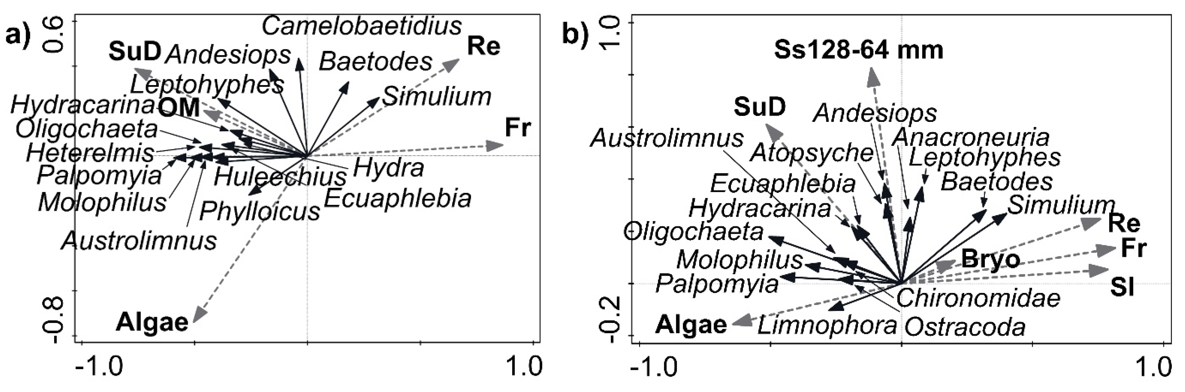
The RDA identified five variables (Fr, SuD, Algae, organic matter content in the sediment, Re) that affected the spatial distribution of the macroinvertebrate communities in the main river (Figure 2;

Table 3. Results of the Redundancy Analysis (RDA) applied on the data of (a) main river; and (b) tributaries. Number of samples considered in the analysis, N = 300 (main river) and N = 297 (tributaries). p = significance value.

(a) Main River
Statistical Parameter	Axis
	1	2	3	4
Eigenvalue	0.104	0.039	0.008	0.005
Explained variation (cumulative)	10.4	14.3	15	15.5
Pseudo-canonical correlation	0.68	0.44	0.40	0.28
Explained fitted variation (cumulative)	66.2	90.8	95.9	98.8
Variable (%)	Explanation (%)	Contribution	pseudo-F	p
Froude number (Fr)	7.9	39.0	25.5	0.002
Shannon-Wiener substrate diversity (SuD)	2.4	11.8	7.9	0.002
Algae coverage (Algae)	2.3	11.3	8.0	0.002
Organic matter	1.6	8.1	5.5	0.002
Reynolds number (Re)	1.5	7.4	5.1	0.002
(b) Tributaries
Statistical parameter	Axis
	1	2	3	4
Eigenvalue	0.066	0.041	0.012	0.008
Explained variation (cumulative)	6.6	10.7	11.9	12.7
Pseudo-canonical correlation	0.71	0.46	0.40	0.37
Explained fitted variation (cumulative)	48.8	79.0	88.1	93.7
Variable	Explanation (%)	Contribution (%)	pseudo-F	p
Froude number (Fr)	4.5	23.9	13.9	0.002
Fine cobble substrate	3.0	15.3	9.4	0.002
Substrate index (SI)	1.5	7.6	4.8	0.002
Reynolds number (Re)	1.3	6.8	4.2	0.002
Shannon-Wiener substrate diversity (SuD)	1.2	6.0	3.8	0.002
Algae coverage (Algae)	1.1	5.4	3.4	0.002
Bryophytes coverage (Bryo)	1.0	5.1	3.3	0.002

). The first axis of RDA explained 10.4% of the variation in the data set and showed a gradient related to Fr and Re. The second axis explained 3.9% of the variation and indicated a gradient related to Algae (Figure 2a; Table 3a). RDA selected 7 significant hydraulic and habitat variables (Fr, fine cobble, SI, Re, SuD, Algae, Bryo) in the tributary dataset. The first axis of RDA explained 6.6% of the variation in the data set and reflected a gradient related to Fr, Re, SI and Bryo.

The second axis explained 4.1% of the variation and indicated a gradient related to fine cobble and SuD (Figure 2b; Table 3b). Palpomyia, Molophilus, Austrolimnius, Oligochaeta taxa were negatively associated with faster flow habitats (i.e., characterised by higher Fr values) in both, the main river and tributaries. Further, in the tributaries they are negatively associated with SI. In contrast, Simulium and Baetodes taxa were positively associated with Re in both channel types. Ecuaphlebia and Hydracarina taxa were positively related to SuD in the tributaries while Hydracarina and Leptohyphes were positively associated to SuD and organic matter content in the sediment in the main river. Leptohyphes, Andesiops, Atopsyche and Anacroneuria were positively related to fine cobble substrate in the tributaries. Limnophora, was positively correlated to Algae in tributaries; similarly, Phylloicus is positively correlated to Algae in the main river.

3.3. Individual Taxa Response to Selected Hydraulic and Habitat Variables

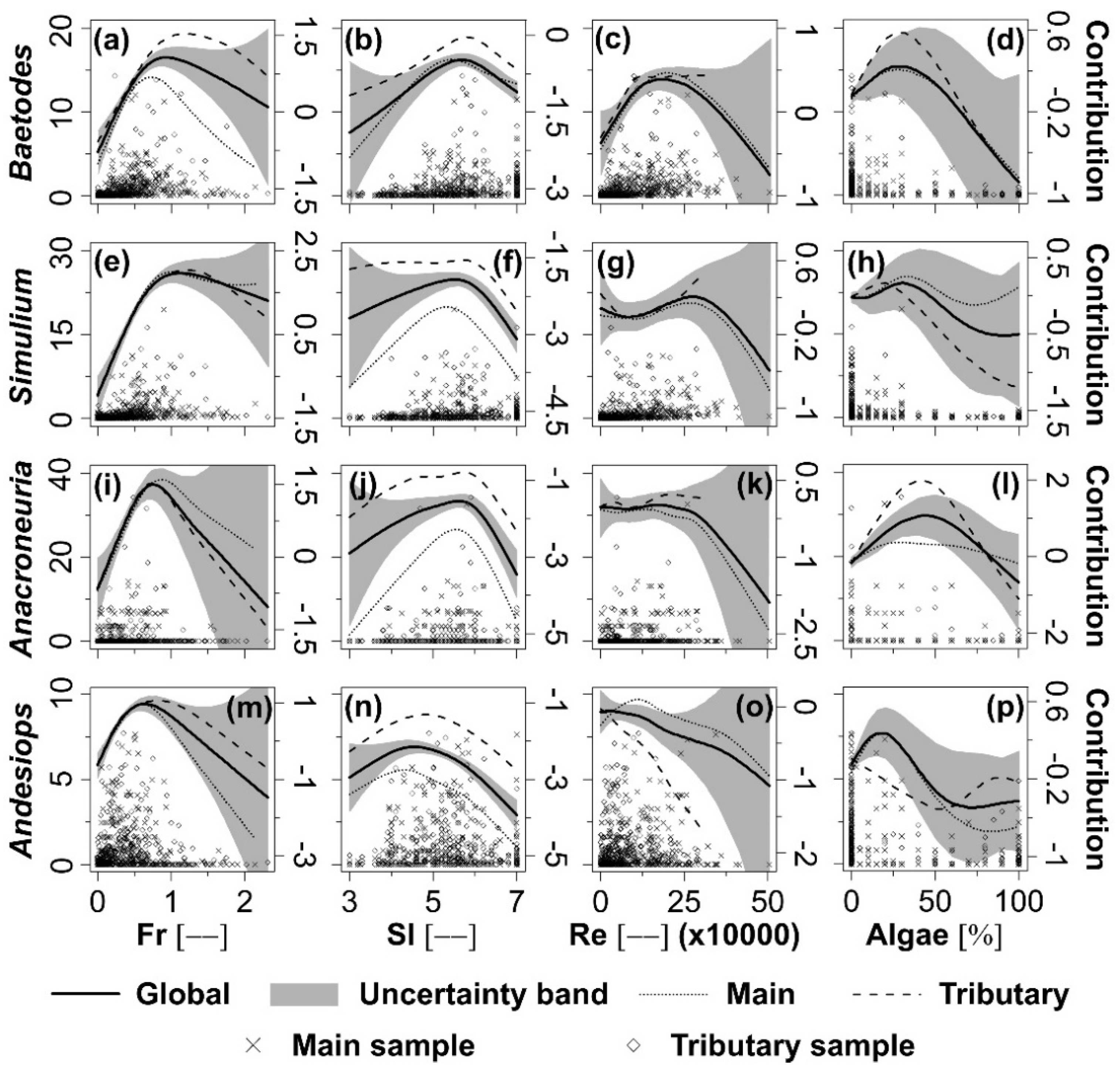
The application of the GAMs method on the standardised densities (δ) of the selected 8 taxa in the Yanuncay River (i.e., global analysis) using only significant variables explained different percentages of the total deviance (

Table 4. Generalised additive models (GAMs) that relate standardised density (δ) of Baetodes, Simulium, Anacroneuria, Andesiops, Camelobaetidius, Ecuaphlebia, Atopsyche, and Palpomyia in the Yanuncay River (global analysis) with Re = Reynolds number, Fr = Froude number, SI = substrate index and Algae = algae coverage. Res. = residual; dev. = deviance; %TD = percentage of total deviance; df = degree of freedom; p = significance value.

	Test for Significance						Test for Non-Linearity
Taxa	Model	Res. dev.	%TD Explained	Res. df	F Ratio	p	Model	Res. dev.	Res. df	F Ratio	p
Baetodes	Null	1192	0.0	596.0
	Fr	970	18.6	594.2	58.8	<0.001	Fr	881	592.9	78.1	<0.001
	Fr + SI	815	31.6	591.0	51.8	<0.001	SI	1043	593.1	39.3	<0.001
	Fr + SI + Re	790	33.7	587.9	36.8	<0.001	Re	937	592.9	61.1	<0.001
	Fr + SI + Re + Algae	781	34.5	585.0	28.7	<0.001	Algae	1105	593.0	24.8	<0.001
Simulium	Null	1336	0.0	590.0
	Fr	1113	16.7	588.3	54.7	<0.001	Fr	1001	587.0	76.8	<0.001
	Fr + SI	920	31.1	585.1	50.6	<0.001	SI	1235	587.1	25.7	<0.001
	Fr + SI + Re	912	31.7	581.8	33.4	<0.001	Re	1163	586.8	36.1	<0.001
	Fr + SI + Re + Algae	903	32.4	578.8	25.7	<0.001	Algae	1274	587.0	18.1	<0.001
Anacroneuria	Null	2443	0.0	595.0
	Fr	2329	4.7	593.3	20.0	<0.001	Fr	2292	592.1	22.0	<0.001
	Fr + SI	2126	13.0	590.0	19.3	<0.001	SI	2246	592.0	25.9	<0.001
	Fr + SI + Re	2106	13.8	586.6	13.0	<0.001	Re	2391	591.8	11.4	<0.001
	Fr + SI + Re + Algae	1994	18.4	583.8	13.1	<0.001	Algae	2388	592.1	12.9	<0.001
Andesiops	Null	1146	0.0	593.0
	Fr	1012	11.7	591.2	29.1	<0.001	Fr	1012	590.1	29.0	<0.001
	Fr + SI	983	14.2	587.9	16.7	<0.001	SI	1007	589.9	28.1	<0.001
	Fr + SI + Re	980	14.5	584.6	11.0	<0.001	Re	1105	589.9	8.4	<0.001
	Fr + SI + Re + Algae	966	15.7	581.5	9.1	<0.001	Algae	1108	590.0	8.1	<0.001
Camelobaetidius	Null	2249	0.0	594.0
	Fr	2041	9.2	592.2	26.4	<0.001	Fr	2039	591.2	25.9	<0.001
	Fr + SI	1971	12.4	589.2	16.6	<0.001	SI	2102	591.1	18.4	<0.001
	Fr + SI + Re	1909	15.1	586.3	13.5	<0.001	Re	2070	591.1	21.6	<0.001
	Fr + SI + Re + Algae	1825	18.9	583.7	13.2	<0.001	Algae	2083	591.4	22.7	<0.001
Ecuaphlebia	Null	1756	0.0	595.0
	Fr	1679	4.4	592.6	10.1	<0.001	Fr	1627	592.7	23.7	<0.001
	Fr + SI	1577	10.2	590.6	13.9	<0.001	SI	1492	592.1	38.9	<0.001
	Fr + SI + Re	1562	11.0	587.7	9.8	<0.001	Re	1699	592.3	9.9	<0.001
	Fr + SI + Re + Algae	1498	14.7	584.7	9.6	<0.001	Algae	1736	592.0	4.7	<0.001
Atopsyche	Null	1439	0.0	593.0
	Fr	1354	5.9	591.2	16.4	<0.001	Fr	1352	590.2	16.3	<0.001
	Fr + SI	1302	9.5	588.1	11.8	<0.001	SI	1341	590.0	17.1	<0.001
	Fr + SI + Re	1262	12.3	585.0	10.1	<0.001	Re	1368	590.0	13.1	<0.001
	Fr + SI + Re + Algae	1252	13.0	581.9	7.9	<0.001	Algae	1415	590.0	5.8	<0.001
Palpomyia	Null	1950	0.0	594.0
	Fr	1686	13.5	591.2	33.6	<0.001	Fr	1623	591.7	65.1	<0.001
	Fr + SI	1677	14.0	589.4	21.8	<0.001	SI	1605	591.0	53.6	<0.001
	Fr + SI + Re	1643	15.7	586.5	16.5	<0.001	Re	1621	591.5	60.5	<0.001
	Fr + SI + Re + Algae	1562	19.9	583.4	15.3	<0.001	Algae	1791	590.9	25.9	<0.001

). In the case of Baetodes and Simulium, the explained percentages of the total deviance were the highest, 34.5% and 32.4%, respectively, for the full GAMs; whilst in case of Ecuaphlebia and Atopsyche the four significant variables explained the lowest percentages of the total deviance (i.e., 14.7% and 13.0%, respectively). Fr explained the highest deviance in the δ of Baetodes, Simulium, Andesiops, Camelobaetidius, Atopsyche and Palpomyia in the GAM model (18.6%, 16.7%, 11.7%, 9.2%, 5.9% and 13.5%, respectively). SI explained the highest deviance in the δ of Anacroneuria and Ecuaphlebia with 8.3% and 5.8%, respectively. Further, the F test (F ratio > 2.5 and p < 0.05) suggested significant non-linear relationships between the δ of all of the 8 studied taxa and Fr, Re, SI and Algae supporting as such the use of non-linear GAMs in the current study.

Baetodes (Figure 3a,b) and Simulium (Figure 3e,f) presented single peaked habitat suitability curves with higher values around Fr = 1.2 and SI = 6.0, respectively; Anacroneuria (Figure 3i,j), in turn, around Fr = 0.7 and SI = 6.0. Standardised densities (δ) of Andesiops peaked around Fr = 0.5 and SI = 4.8 (Figure 3m,n). The habitat suitability curves of Baetodes (Figure 3c), Simulium (Figure 3g) and Andesiops (Figure 3o) exhibited maximum δ around Re values of 140,000, 270,000 and 40,000 respectively. Anacroneuria (Figure 3k) presented a top flatted curve till approximately Re = 230,000, after which, it started to decline. Baetodes, Simulium and Anacroneuria had higher δ around 35%, 35% and 45% of Algae, respectively (Figure 3d,h,l). Andesiops had different tendencies as a function of the channel type; it had peak δ at 15% of Algae in the main river while showed higher δ at low (about 0%) and high (80%) Algae in the tributaries (Figure 3p). Tendencies and peak values of the four variables are very similar in the main river and tributaries, except for the Algae in the case of Andesiops.

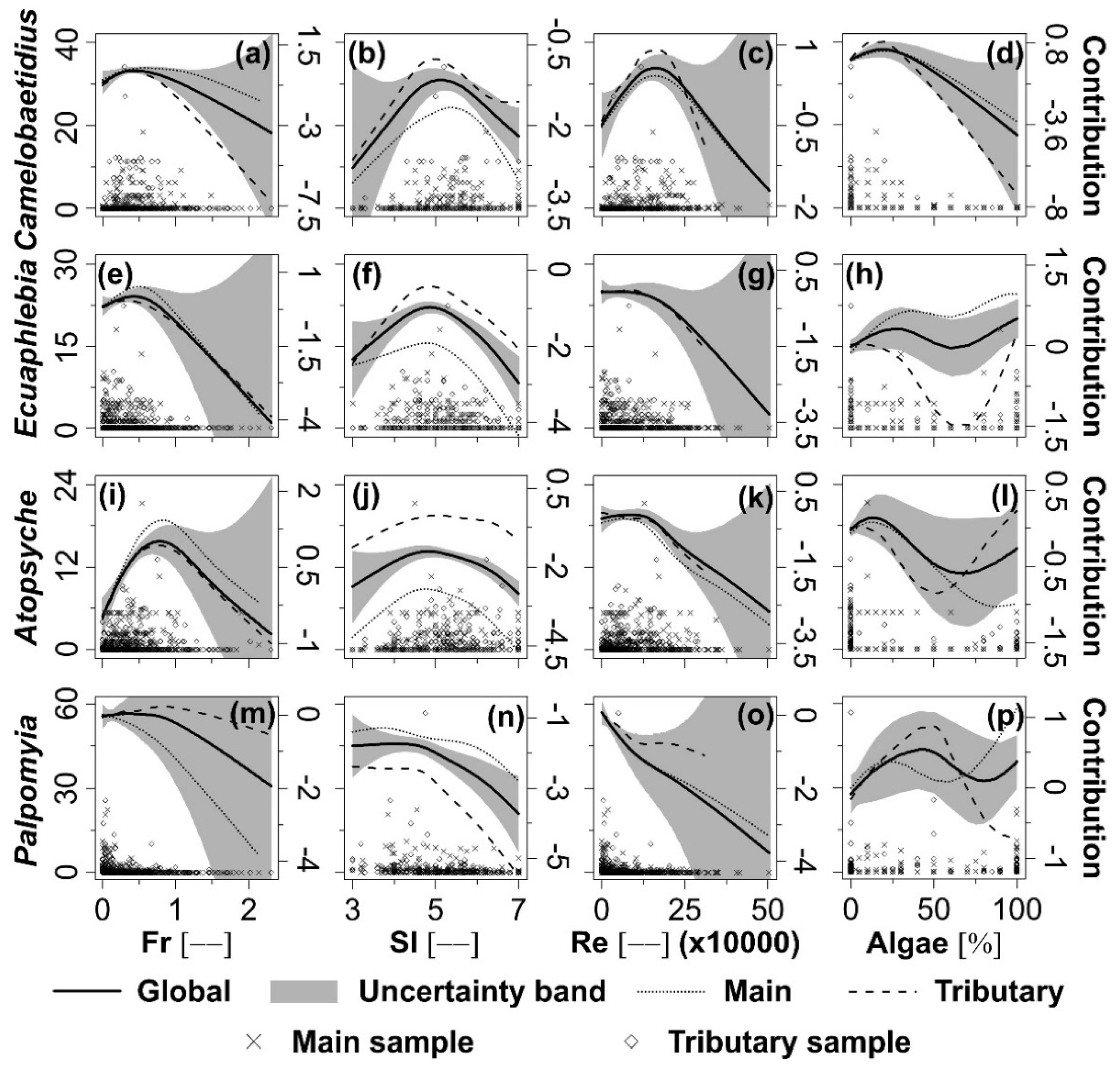
Camelobaetidius (Figure 4a–c) had density peaks at about Fr = 0.4, SI = 5.0 and Re = 160,000, respectively. The standardised density (δ) of Ecuaphlebia peaked at around Fr = 0.4 (Figure 4e) and SI = 4.9 (Figure 4f); and exhibited a negative relation with Re (Figure 4g). Atopsyche genus δ peaked (Figure 4i–k) at about Fr = 0.9, SI = 5.0 and Re = 120,000. The Palpomyia genus’ δ decreased with Fr (Figure 4m) and Re (Figure 4o) and reached maximum values around SI = 4 (Figure 4n). The δ response of these four genera to Fr, SI and Re was similar in the main river and tributaries. The δ of Camelobaetidius had a decreasing relation with Algae (Figure 4d). Ecuaphlebia (Figure 4h) had lowest δ at intermediate Algae (about 60%) in both channel types. Atopsyche (Figure 4l) and Palpomyia (Figure 4p) did not show clear trend as response to this variable; moreover, response of these taxa to Algae varied importantly between the main river and the tributaries.

Seeking clarity, Figure 3 and Figure 4 depict only the confidence band encompassing the global habitat suitability curves. In general, there was less confidence in the regions of the habitat suitability curves where standardised density data were scarce, indicated by increased width of the confidence bands (Figure 3 and Figure 4).

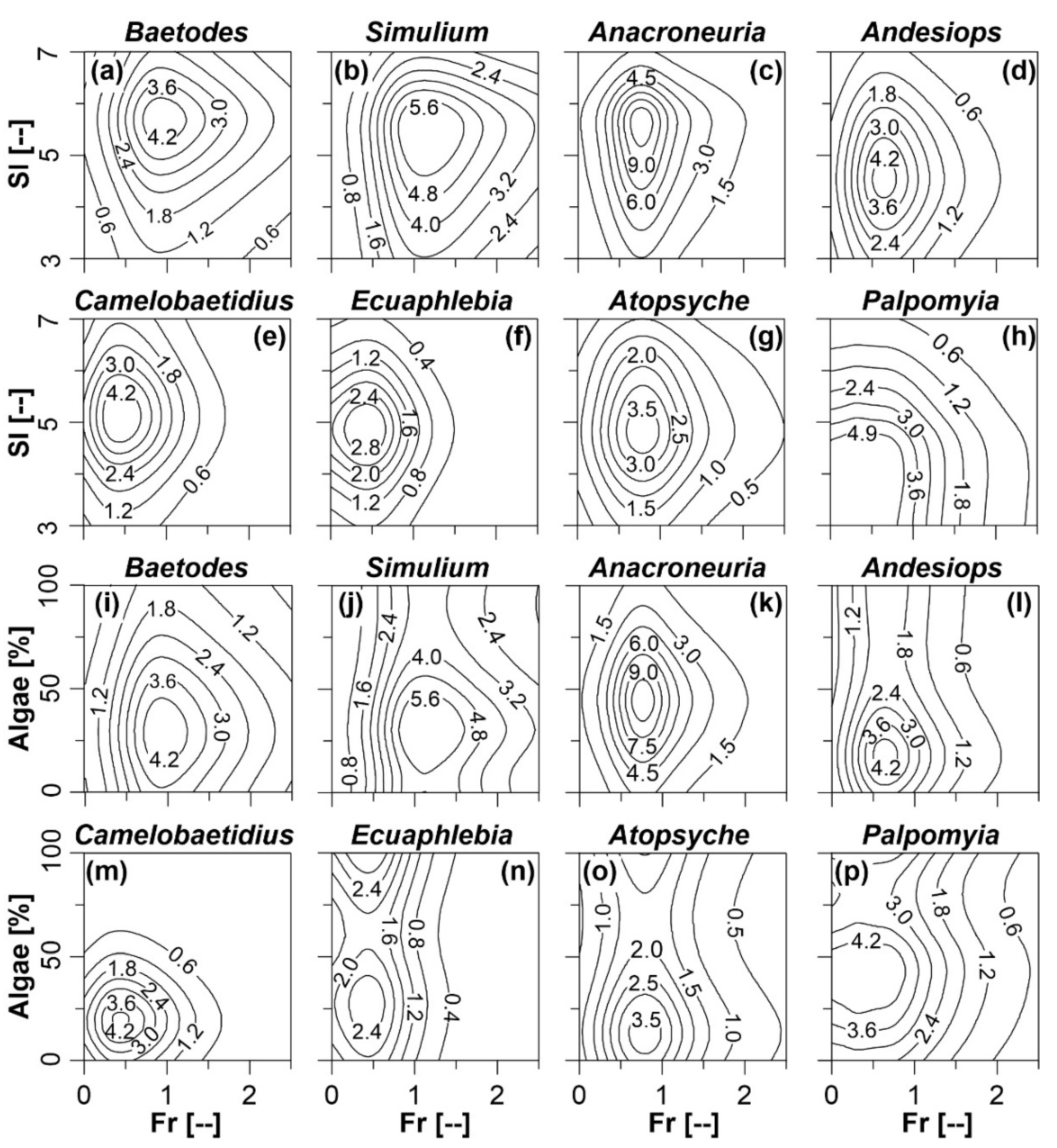
Figure 5 illustrates the standardised density (δ) contour curves of the different taxa as a function of Fr-SI and of Fr-Algae, as described by the full GAMs. High response δ of the genera Baetodes (Figure 5a), Simulium (Figure 5b) and Anacroneuria (Figure 5c) occurred in habitats characterised by Fr > 0.5 and larger substrate sizes. Atopsyche (Figure 5g) was present in habitats with Fr > 0.5 but smaller substrate sizes. Andesiops (Figure 5d) Camelobaetidius (Figure 5e), Ecuaphlebia (Figure 5f) happened in habitats with Fr < 0.5 and larger substrate sizes. The Palpomyia genus (Figure 5h) occurred in quiet habitats (Fr < 0.25) and smaller substrate sizes.

Baetodes (Figure 5i) and Simulium (Figure 5j) were present in habitats with higher Fr (i.e., Fr > 1.0) but with lower Algae (about 30%). Higher standardised density (δ) values of Anacroneuria (Figure 5k) and Atopsyche (Figure 5o) were found in habitats with Fr > 0.5 and Algae around 50% and 15%, respectively. Andesiops (Figure 5l), Camelobaetidius (Figure 5m) and Ecuaphlebia (Figure 5n) were restricted to habitats with Fr < 0.5 and little Algae while Palpomyia (Figure 5p) was concentrated in habitats with Fr < 0.25 and Algae of about 40%.

4. Discussion

The current study analysed the response of aquatic macroinvertebrates to hydraulic and habitat variability occurring at the microhabitat scale. Macroinvertebrate communities were sampled at habitats distributed along the main and tributary channels of the Yanuncay River, at different flow conditions. 597 samples were included to obtain robust results. Environmental conditions at the macro- and micro-scales were measured/calculated. At the macro-scale, physical-chemical variables, slope, etc. can represent filters for the composition of macroinvertebrate community [10] and for the distribution of certain taxa; similarly to the role of habitat and hydraulic variables at the microhabitat scale.

4.1. Variables Influencing Macroinvertebrate Distribution at the Microhabitat Scale

Hydraulic and habitat characteristics (Fr, Re and substrate size) are important for determining the spatial distribution of aquatic taxa at the micro-scale [14,15,54]. The distribution of taxa in rivers depends on the capacity of its organisms to occupy different habitats, which, in turn, depends on their body structure (i.e., nails, gills, suction cups, etc.) or shape (hydrodynamic, cylindrical or flattened) developed to persist in a particular habitat [60,61,62].

In this study, Simulium, Anacroneuria and Baetodes genera were found in habitats with faster and turbulent flows, which is likely the result of their specific adaptations to this environment. The resistance capacity of Simulium to faster flows is related to the presence of a circular hook structure in the last body segment [63], which allows the organism to be fixed to the bottom of the river bed. Likewise, organisms of the Baetodes genus have hydrodynamic shape, small size and tarsal nails to hold onto the substrate, allowing significant resistance to faster currents [64]. Similarly, the organisms in the genus Anacroneuria have strong and flattened body structure [65] against strong current, while Camelobaetidius has a hydrodynamic shape and cushion legs [66]. Both, Anacroneuria and Camelobaetidius, typically occur in habitats with fast currents; nevertheless, in this study Camelobaetidius preferred slower flows.

Palpomyia, Molophilus, Phylloicus and Oligochaeta are characterised by the absence of specific body structures or adaptive body form to high currents; hence, they are prone to be negatively affected by faster flows. Further, these groups are frequent in low flow areas (pools) where fine sediment and OM accumulate [7,10,67], which was also observed in this study. Herein, Huleechius were present in habitats of the main river with slower flow and higher OM, in contradiction to the results from the study of Ríos-Pulgarín et al. [64] applied on a high mountain river. Furthermore, Austrolimnius was also present in the main river and tributary habitats characterised by lower flow and higher OM conditions, which is similar to what was found by González-Trujillo and Donato-Rondon [68] that carried out a study above 3500 m a.s.l.

Another influential variable in the habitat distribution of certain aquatic taxa is the diversity or heterogeneity of substrate (SuD). Generally, organisms prefer substrates of different sizes, which provide them better refuge against different flow conditions or predators [69,70]. RDA showed that Hydracarina was associated to these refuge habitats with diverse substrate from which organisms could find further refuge in the hyporheic zones at extreme (high or low) flow events [71]. Ecuaphlebia, belonging to the Leptophlebidae family, was also present in heterogenic substrate likely using these sites as refuge, similarly to what was observed in other latitudes by Dostine et al. [71] with respect to the Leptophlebidae family. On the other hand, Cobb et al. [72] refers to the fact that large substrates provide stable habitat to aquatic insects; this has been observed in this study specially in the tributaries for Leptohyphes, Andesiops and Atopsyche that preferred the (128–64 mm) thick substrate.

4.2. Individual Taxa Response to Selected Hydraulic and Habitat Variables

The above refers to the RDA results that outlined linear responses of certain taxa to hydraulic and substrate variables. Furthermore, habitat suitability curves of taxa for certain microhabitat conditions were developed using GAMs. Herein, the observed preference of the Simulium genus for sites with faster and turbulent flow is consistent with the results of the study of Palmer et al. [73]. Simulium fixes its body to a thick substrate and takes advantage of faster flow by filtering water for capturing suspended food particles; however, in small channels these organisms are opportunistic and quickly adapt to different conditions [74]. Anacroneuria is also well adapted to faster flow and turbulent habitats as indicated by the respective habitat suitability curve. In Andean rivers Anacroneuria has feeding preference for the genus Simulium [75]. However, in this study Anacroneuria standard density decreased more rapidly than the Simulium standardised density under faster flow conditions; hence, these habitats could represent refuge for this genus against predation.

Baetodes are herbivorous [76]; they were present in habitats with faster flow (i.e., Fr > 0.5), which results in a lower coverage of filamentous algae. This genus is likely to have a feeding habit specialised on algae species resistant to fast flow. Atopsyche is mainly predator [77] and its feeding strategy is supported by faster flow but less turbulent habitats with large substrate sizes. Ecuaphlebia genus was present mainly in lower velocity habitats with intermediate substrate size, which contradicts the findings of Vimos-Lojano et al. [78] that refers to Ecuaphlebia being present in habitats with faster currents and larger substrate in an Andean subcatchment with elevations higher than 3500 m of elevation. The genus Andesiops, despite having a hydrodynamic form for swimming and tarsal nails for attaching to the substrate [77] do not frequent faster and turbulent flow environments. Population-genetic structure of Andesiops was studied by Finn et al. [79]; however, more detailed studies of this genus are needed, given the dominance of this genus in the Andean region and its potential ecological importance.

The low resistance to high flows of Camelobaetidius and Palpomyia is mainly due to their biological features that are poorly adapted to strong currents [77,80]; hence, these groups are frequent in areas of pools or slow flow. According to Tomanova et al. [77] Camelobaetidius can be scraper or collector-gatherer; in the Yanuncay sub-basin this genus most probably has the latter behaviour because it is present in habitats with low algae coverage. Palpomyia could be either predator, scraper or collector-gatherer [77]. In this study, this genus occupied habitats with small substrate and intermediate or large algae coverage, which suggests scraper and collector-gatherer feeding habits.

The current study revealed very few differences in hydraulic and habitat responses of the studied taxa for Fr, SI and Re as a function of channel types (i.e., main river and tributaries). These findings contradict other studies. Jowett [34] indicated a scaling effect in hydraulic responses for macroinvertebrates in New Zealand rivers, with preferred depths and mean velocities in small streams being considerably lower than those noticed for large rivers. Furthermore, Mérigoux et al. [81] revealed differences in hydraulic responses of macroinvertebrates between small and large streams; as such, they questioned the transferability of models of hydraulic habitat responses between rivers. In the current study, the relatively short spatial distance between the sampling stations located at the main river and tributaries and their similar characteristics are likely to have resulted in studied taxa exhibiting very similar responses to the previously mentioned hydraulic and habitat variables.

Hydropower projects are rapidly increasing in the Neotropics. In the Andean region, around 50% of new dams are classified as high impact (i.e., major break in river connectivity, deforestation, threaten to biodiversity, etc.) and just 19% as low impact [25,82]. Owing to climate change, glaciers in the tropical Andes have been retreating for the past several decades, leading to a shortage of water supply downstream [83]. Moreover, in the Paute river basin, where the study site is located, increasing peak flows and decreasing low flows are expected in the future because of climate change [84].

A dam construction is planned in the near future in the upper part of the study sub-basin as well as climate and land use changes are expected to happen in the mid-term, which will likely result in hydrological/hydraulic alteration in the studied river with various consequences on associated ecosystems. Henceforth, macroinvertebrate taxa that need higher discharge, faster flow and more turbulent flow conditions might disappear (i.e., Baetodes, Simulium, Anacroneuria and Atopsyche) to give space to taxa that are linked to slow flow conditions (i.e., Palpomyia, Oligochaeta, Molophilus).

Further, since flow regime controls the occurrence of algae, dam regulated flow could lead to an increase of biomass and density of some filamentous algae [85] and, as such, might impact macroinvertebrate communities, for instance, increasing the abundance of taxa, which have scraper feeding habit, or might result in the change of feeding habits. For instance, Camelobaetidius is most probably collector-gatherer in the studied river but with different algal coverage it might shift its feeding habit to scraper. Algal coverage change might alter ecosystem functioning by modifying the distribution and abundance of the base of the aquatic food web [86].

To maintain hydrological/hydraulic conditions for protecting river biota and good ecological status of the studied river, direct physical changes including sand extraction or river straightening need to be strongly under control. Further, in the view of future hydrological/hydraulic changes owing to dam construction and operation, environmental flow regime needs to be established through the incorporation of data on flow-ecology relationships into operational use of environmental flow definition [85].

5. Conclusions

This study was carried out in the Yanuncay sub-basin, southern Ecuador. However, despite the fact that results achieved cannot be directly transferred, they may be considered in other similar studies applied in Andean aquatic systems. Knowledge of the hydraulic-habitat response of macroinvertebrates at the microhabitat scale is important for a more holistic determination of environmental flows; however, this knowledge is still poor in the Andean context.

Eight hydraulic and habitat variables (SI, Fr, Re, Algae, fine cobble, SuD, Bryo and organic matter content in the sediment) were regarded as influencing the distribution of aquatic macroinvertebrate communities in the main river and tributaries. Further, GAMs were used to depict microhabitat responses of several macroinvertebrate taxa in terms of these hydraulic and habitat variables. The analysis showed more meaningful habitat suitability curves only for Fr, Re, SI and Algae. Eight taxa were selected as response variables in the GAMs analysis based on their high occurrence and dominance in the samples, their sensitivity to river water quality, their significance in the RDA and their meaningful response in the GAMs. Baetodes and Simulium had flow preferences represented by Fr > 1.0 and larger substrate size while Anacroneuria had similar habitat preference for the substrate though for slightly slower flow (0.5 < Fr < 1.0). Andesiops, Camelobaetidius and Ecuaphlebia preferred slower flow (0.5 < Fr) though still large substrate. On the other hand, Palpomyia had affinity to lentic areas with small substrate size. Algae influenced the presence of certain taxa (i.e., Baetodes, Camelobaetidius, Palpomyia) in connection with their scraper or collector-gatherer feeding habits. Atopsyche is mainly predator and its feeding strategy is supported by faster flow but less turbulent habitats with large substrate sizes. Baetodes, Simulium, Anacroneuria and Atopsyche taxa could be affected in case of discharge reduction by human activities (i.e., the presence and operation of dams). Palpomyia could be affected by sudden increase of discharge resulting from natural flood events or water released from dams.

The results of this study contributed to the scientific knowledge of the hydraulic responses of aquatic organisms, which is necessary to design predictive models for quantifying the necessary flow regimes aiming at maintaining biotic and abiotic processes within river systems. Future studies should focus on physical habitat modelling and environmental flow analysis using the eco-hydraulic knowledge of aquatic taxa developed in this and similar studies, as a contribution to better water resources management in the Andean region. In general, there was less confidence in the regions of the generated habitat suitability curves where standardised density data were scarce. This should be considered when using the generated habitat suitability curves in the scope of further analyses, particularly, habitat modelling.

References

- Uribe, N.; Srinivasan, R.; Corzo, G.; Arango, D.; Solomatine, D. Spatio-temporal critical source area patterns of runoff pollution from agricultural practices in the Colombian Andes. Ecol. Eng. 2020, 149, 105810. [Google Scholar] [CrossRef]
- Miserendino, M.L.; Pizzolon, L.A. Interactive effects of basin features and land-use change on macroinvertebrate communities of headwater streams in the Patagonian Andes. River Res. Appl. 2004, 20, 967–983. [Google Scholar] [CrossRef]
- Durance, I.; Ormerod, S.J. Climate change effects on upland stream macroinvertebrates over a 25-year period. Glob. Chang. Biol. 2007, 13, 942–957. [Google Scholar] [CrossRef]
- Bo, T.; Piano, E.; Doretto, A.; Bona, F.; Fenoglio, S. Microhabitat preference of sympatric Hydraena Kugelann, 1794 species (Coleoptera: Hydraenidae) in a low-order forest stream. Aquat. Insects 2017, 37, 287–292. [Google Scholar] [CrossRef]
- Li, F.; Cai, Q.; Fu, X.; Liu, J. Construction of habitat suitability models (HSMs) for benthic macroinvertebrate and their applications to instream environmental flows: A case study in Xiangxi River of Three Gorges Reservior region, China. Prog. Nat. Sci. 2009, 19, 359–367. [Google Scholar] [CrossRef]
- Bedoya, D.; Manolakos, E.S.; Novotny, V. Characterization of biological responses under different environmental conditions: A hierarchical modeling approach. Ecol. Model. 2011, 222, 532–545. [Google Scholar] [CrossRef]
- Schröder, M.; Kiesel, J.; Schattmann, A.; Jähnig, S.C.; Lorenz, A.W.; Kramm, S.; Keizer-Vlek, H.; Rolauffs, P.; Graf, W.; Leitner, P.; et al. Substratum associations of benthic invertebrates in lowland and mountain streams. Ecol. Indic. 2013, 30, 178–189. [Google Scholar] [CrossRef]
- Serpa, K.V.; Kiffer, W.P.; Borelli, M.F.; Ferraz, M.A.; Moretti, M.S. Niche breadth of invertebrate shredders in tropical forest streams: Which taxa have restricted habitat preferences? Hydrobiologia 2019, 847, 1739–1752. [Google Scholar] [CrossRef]
- Parsons, M.; Norris, R. The effect of habitat-specific sampling on biological assessment of water quality using a predictive model. Freshw. Biol. 1996, 36, 419–434. [Google Scholar] [CrossRef]
- Vimos-Lojano, D.; Martínez-Capel, F.; Hampel, H. Riparian and microhabitat factors determine the structure of the EPT community in Andean headwater rivers of Ecuador. Ecohydrology 2017, 10, e1894. [Google Scholar] [CrossRef] [Green Version]
- Collier, K.J. Flow preferences of larval Chironomidae (Diptera) in Tongariro River, New Zealand. N. Z. J. Mar. Freshw. Res. 1993, 27, 219–226. [Google Scholar] [CrossRef]
- Degani, G.; Herbst, G.N.; Ortal, R.; Bromley, H.J.; Levanon, D.; Netzer, Y.; Harari, N.; Glazman, H. Relationships between current velocity, depth and the invertebrate community in a stable river system. Hydrobiologia 1993, 263, 163–172. [Google Scholar] [CrossRef]
- Guevara-Mora, M.; Pedreros, P.; Urrutia, R.; Figueroa, R. Efectos de la extracción agrícola del agua en el hábitat fluvial de macroinvertebrados bentónicos en Chile. Hidrobiológica 2016, 26, 373–382. [Google Scholar] [CrossRef] [Green Version]
- Mérigoux, S.; Dolédec, S. Hydraulic requirements of stream communities: A case study on invertebrates. Freshw. Biol. 2004, 49, 600–613. [Google Scholar] [CrossRef]
- Statzner, B.; Gore, J.A.; Resh, V.H. Hydraulic stream ecology: Observed patterns and potential applications. J. N. Am. Benthol. Soc. 1988, 7, 307–360. [Google Scholar] [CrossRef]
- Shearer, K.; Hayes, J.; Jowett, I.; Olsen, D. Habitat suitability curves for benthic macroinvertebrates from a small New Zealand river. N. Z. J. Mar. Freshw. Res. 2015, 49, 178–191. [Google Scholar] [CrossRef]
- Kim, S.K.; Choi, S.-U. Ecological evaluation of weir removal based on physical habitat simulations for macroinvertebrate community. Ecol. Eng. 2019, 138, 362–373. [Google Scholar] [CrossRef]
- Mesa, L.M. Hydraulic parameters and longitudinal distribution of macroinvertebrates in a subtropical Andean basin. Interciencia 2010, 35, 759–764. [Google Scholar]
- Jerves-Cobo, R.; Everaert, G.; Iñiguez-Vela, X.; Córdova-Vela, G.; Díaz-Granda, C.; Cisneros, F.; Nopens, I.; Goethals, P.L. A methodology to model environmental preferences of EPT taxa in the Machangara River Basin (Ecuador). Water 2017, 9, 195. [Google Scholar] [CrossRef] [Green Version]
- Masikini, R.; Kaaya, L.T.; Chicharo, L. Evaluation of ecohydrological variables in relation to spatial and temporal variability of macroinvertebrate assemblages along the Zigi River–Tanzania. Ecohydrol. Hydrobiol. 2018, 18, 130–141. [Google Scholar] [CrossRef]
- Holzapfel, P.; Leitner, P.; Habersack, H.; Graf, W.; Hauer, C. Evaluation of hydropeaking impacts on the food web in alpine streams based on modelling of fish- and macroinvertebrate habitats. Sci. Total Environ. 2017, 575, 1489–1502. [Google Scholar] [CrossRef] [PubMed]
- Monk, W.A.; Compson, Z.G.; Armanini, D.G.; Orlofske, J.M.; Curry, C.J.; Peters, D.L.; Crocker, J.B.; Baird, D.J. Flow velocity–ecology thresholds in Canadian rivers: A comparison of trait and taxonomy-based approaches. Freshw. Biol. 2017, 63, 891–905. [Google Scholar] [CrossRef]
- Asamblea-Nacional. Ley Orgánica de Recursos Hídricos, Usos y Aprovechamiento del Agua; Asamblea-Nacional: Quito, Ecuador, 2014. [Google Scholar]
- MINAMBIENTE IDEAM. Guía Metodológica para la Estimación del Caudal Ambiental; Ministerio de Ambiente y Desarrollo Sostenible (MINAMBIENTE), Meteorología y Estudios Ambientales Instituto de Hidrología, Eds.; MINAMBIENTE IDEAM: Bogotá, Colombia, 2017. [Google Scholar]
- Anderson, E.P.; Jenkins, C.N.; Heilpern, S.; Maldonado-Ocampo, J.A.; Carvajal-Vallejos, F.M.; Encalada, A.C.; Rivadeneira, J.F.; Hidalgo, M.; Cañas, C.M.; Ortega, H.; et al. Fragmentation of Andes-to-Amazon connectivity by hydropower dams. Sci. Adv. 2018, 4, eaao1642. [Google Scholar] [CrossRef] [PubMed] [Green Version]
- Borja, P.; Molina, A.; Govers, G.; Vanacker, V. Check dams and afforestation reducing sediment mobilization in active gully systems in the Andean mountains. Catena 2018, 165, 42–53. [Google Scholar] [CrossRef]
- Gore, J.A.; Judy, R.D. Predictive models of benthic macroinvertebrate density for use in instream flow studies and regulated flow management. Can. J. Fish. Aquat. Sci. 1981, 38, 1363–1370. [Google Scholar] [CrossRef]
- Theodoropoulos, C.; Vourka, A.; Skoulikidis, N.; Rutschmann, P.; Stamou, A. Evaluating the performance of habitat models for predicting the environmental flow requirements of benthic macroinvertebrates. J. Ecohydraulics 2018, 3, 30–44. [Google Scholar] [CrossRef]
- Kelly, D.J.; Hayes, J.W.; Allen, C.; West, D.; Hudson, H. Evaluating habitat suitability curves for predicting variation in macroinvertebrate biomass with weighted usable area in braided rivers in New Zealand. N. Z. J. Mar. Freshw. Res. 2015, 49, 398–418. [Google Scholar] [CrossRef]
- Muñoz-Mas, R.; Papadaki, C.; Martínez-Capel, F.; Zogaris, S.; Ntoanidis, L.; Dimitriou, E. Generalized additive and fuzzy models in environmental flow assessment: A comparison employing the West Balkan trout (Salmo farioides; Karaman, 1938). Ecol. Eng. 2016, 91, 365–377. [Google Scholar] [CrossRef]
- Ahmadi-Nedushan, B.; St-Hilaire, A.; Bérubé, M.; Robichaud, É.; Thiémonge, N.; Bobée, B. A review of statistical methods for the evaluation of aquatic habitat suitability for instream flow assessment. River Res. Appl. 2006, 22, 503–523. [Google Scholar] [CrossRef]
- Payne, T.R.; Jowett, I. SEFA—Computer Software System for Environmental Flow Analysis Based on the Instream Flow Incremental Methodology. In Proceedings of the 2013 Georgia Water Resources Conference, Athens, Georgia, 10–11 April 2013. [Google Scholar]
- Lamouroux, N.; Jowett, I.G. Generalized instream habitat models. Can. J. Fish. Aquat. Sci. 2005, 62, 7–14. [Google Scholar] [CrossRef]
- Jowett, I.G. Flow management. In New Zealand Stream Invertebrates: Ecology and Implications for Management; Collier, K., Winterbourn, M., Eds.; New Zealand Limnological Society: Christchurch, New Zealand, 2000; pp. 289–312. ISBN 0473066793. [Google Scholar]
- Jowett, I.G. Hydraulic constraints on habitat suitability for benthic invertebrates in gravel-bed rivers. River Res. Appl. 2003, 19, 495–507. [Google Scholar] [CrossRef]
- Lancaster, J.; Downes, B.J. Linking the hydraulic world of individual organisms to ecological processes: Putting ecology into ecohydraulics. River Res. Appl. 2010, 26, 385–403. [Google Scholar] [CrossRef]
- Lamouroux, N.; Olivier, J.M.; Persat, H.; PouilLy, M.; Souchon, Y.; Statzner, B. Predicting community characteristics from habitat conditions: Fluvial fish and hydraulics. Freshw. Biol. 1999, 42, 275–299. [Google Scholar] [CrossRef]
- Vázquez, R.F.; Célleri, R.; Samaniego, E.; Vanegas, P.; Orellana, J.; Campozano, L.; Vázquez, A.; Avilés, A. Informe Final del Proyecto: “Gestión de Datos y Modelación Hidrológica Para Soporte al Pronóstico de Alerta Temprana del Sistema Paute Integral”; Universidad de Cuenca: Cuenca, Ecuador, 2012; p. 187. [Google Scholar]
- Studholme, A.M.; Hampel, H.; Finn, D.S.; Vázquez, R.F. Secondary production of caddisflies reflects environmental heterogeneity among tropical Andean streams. Hydrobiologia 2017, 797, 231–246. [Google Scholar] [CrossRef]
- Sotomayor, G.; Hampel, H.; Vázquez, R.F.; Goethals, P.L.M. Multivariate-statistics based selection of a benthic macroinvertebrate index for assessing water quality in the Paute River basin (Ecuador). Ecol. Indic. 2020, 111, 106037. [Google Scholar] [CrossRef] [Green Version]
- Sierra, R. Propuesta Preliminar de un Sistema de Clasificación de Vegetación Para el Ecuador Continental; Proyecto INEFAN/GEF-BIRF y Ecociencia: Quito, Ecuador, 1999; p. 174. [Google Scholar]
- Tenesaca, C.; Quinde, T.; Delgado, G.; Toledo, E.; Delgado, O. Generación del mapa de cobertura y uso del suelo de la provincia del Azuay. Univ. Verdad 2017, 73, 23–37. [Google Scholar]
- Boiten, W. Hydrometry: IHE Delft Lecture Note Series; CRC Press: Boca Raton, FL, USA, 2008; p. 244. ISBN 0415467632. [Google Scholar]
- Blair, T.C.; McPherson, J.G. Grain-size and textural classification of coarse sedimentary particles. J. Sediment. Res. 1999, 69, 6–19. [Google Scholar] [CrossRef]
- Domínguez, E.; Fernández, H.R.; Lillo, F.M. Macroinvertebrados Bentónicos Sudamericanos: Sistemática y Biología; Fundación Miguel Lillo Tucumán: Tucumán, Argentina, 2009; p. 656. ISBN 9506680159. [Google Scholar]
- Steinman, A.D.; Lamberti, G.A.; Leavitt, P.R.; Uzarski, D.G. Biomass and pigments of benthic algae. In Methods in Stream Ecology, 3rd ed.; Richard Hauer, F., Lamberti, G.A., Eds.; Elsevier: Amsterdam, The Netherlands, 2017; pp. 223–241. ISBN 978-0-12-416558-8. [Google Scholar]
- Kennen, J.G.; Riva-Murray, K.; Beaulieu, K.M. Determining hydrologic factors that influence stream macroinvertebrate assemblages in the northeastern US. Ecohydrology 2010, 3, 88–106. [Google Scholar] [CrossRef]
- Jowett, I.G. A method for objectively identifying pool, run, and riffle habitats from physical measurements. N. Z. J. Mar. Freshw. Res. 1993, 27, 241–248. [Google Scholar] [CrossRef]
- Rempel, L.L.; Richardson, J.S.; Healey, M.C. Macroinvertebrate community structure along gradients of hydraulic and sedimentary conditions in a large gravel-bed river. Freshw. Biol. 2000, 45, 57–73. [Google Scholar] [CrossRef]
- Masad, J.A. On the Roughness Reynolds Number Transition Criterion. J. Fluids Eng. 1995, 117, 727–729. [Google Scholar] [CrossRef]
- Wilkes, M.A.; Maddock, I.; Visser, F.; Acreman, M.C. Incorporating hydrodynamics into ecohydraulics: The role of turbulence in the swimming performance and habitat selection of stream-dwelling fish. In Ecohydraulics: An Integrated Approach; Maddock, I., Harby, A., Kemp, P., Wood, P.J., Eds.; John Wiley & Sons, Ltd.: Hoboken, NJ, USA, 2013; pp. 9–30. [Google Scholar]
- Brooks, A.J.; Haeusler, T.; Reinfelds, I.; Williams, S. Hydraulic microhabitats and the distribution of macroinvertebrate assemblages in riffles. Freshw. Biol. 2005, 50, 331–344. [Google Scholar] [CrossRef]
- Boyero, L. The quantification of local substrate heterogeneity in streams and its significance for macroinvertebrate assemblages. Hidrobiológica 2003, 499, 161–168. [Google Scholar] [CrossRef]
- Jowett, I.G.; Richardson, J.; Biggs, B.J.; Hickey, C.W.; Quinn, J.M. Microhabitat preferences of benthic invertebrates and the development of generalised Deleatidium spp. habitat suitability curves, applied to four New Zealand rivers. N. Z. J. Mar. Freshw. Res. 1991, 25, 187–199. [Google Scholar] [CrossRef] [Green Version]
- Lepš, J.; Šmilauer, P. Multivariate Analysis of Ecological Data Using CANOCO; Cambridge University Press: Cambridge, UK, 2003; p. 110. ISBN 0521891086. [Google Scholar]
- Šmilauer, P.; Lepš, J. Multivariate Analysis of Ecological Data Using CANOCO 5; Cambridge University Press: Cambridge, UK, 2014; p. 362. ISBN 110769440X. [Google Scholar]
- Ter-Braak, C.J.; Šmilauer, P. Canoco Reference Manual and User’s Guide: Software for Ordination (Vol. Version 5.0); Microcomputer Power: Ithaca, NY, USA, 2012. [Google Scholar]
- Acosta, R.; Ríos, B.; Rieradevall, M.; Prat, N. Propuesta de un protocolo de evaluación de la calidad ecológica de ríos andinos (CERA) y su aplicación a dos cuencas en Ecuador y Perú. Limnetica 2009, 28, 35–64. [Google Scholar]
- Jowett, I.G.; Davey, A.J. A comparison of composite habitat suitability indices and generalized additive models of invertebrate abundance and fish presence–habitat availability. Trans. Am. Fish. Soc. 2007, 136, 428–444. [Google Scholar] [CrossRef]
- Statzner, B. How views about flow adaptations of benthic stream invertebrates changed over the last century. Int. Rev. Hydrobiol. 2008, 93, 593–605. [Google Scholar] [CrossRef]
- Eveleens, R.A.; McIntosh, A.R.; Warburton, H.J. Interactive community responses to disturbance in streams: Disturbance history moderates the influence of disturbance types. Oikos 2019, 128, 1170–1181. [Google Scholar] [CrossRef]
- Waringer, J.; Vitecek, S.; Martini, J.; Zittra, C.; Handschuh, S.; Vieira, A.; Kuhlmann, H.C. Hydraulic stress parameters of a cased caddis larva (Drusus biguttatus) using spatio-temporally filtered velocity measurements. Hidrobiológica 2020, 847, 3437–3451. [Google Scholar] [CrossRef]
- Crosskey, R.W. The identification of the larvae of African Simulium. Bull. Word Health Organ. 1962, 27, 483–489. [Google Scholar]
- Ríos-Pulgarín, M.I.; Barletta, M.; Arango-Jaramillo, M.C.; Mancera-Rodríguez, N.J. The role of the hydrological cycle on the temporal patterns of macroinvertebrate assemblages in an Andean foothill stream in Colombia. J. Limnol. 2016, 75 (Suppl. 1), 107–120. [Google Scholar] [CrossRef] [Green Version]
- Gutierrez-Fonseca, P.E.; Springer, M. A new species of Anacroneuria Klapálek 1909 (Plecoptera: Perlidae) and notes on the altitudinal distribution of the genus in Costa Rica. Zootaxa 2015, 4058, 595–600. [Google Scholar] [CrossRef] [PubMed]
- Forero-Céspedes, A.M.; Gutiérrez, C.; Reinoso-Flórez, G. Composición y estructura de la familia Baetidae (Insecta: Ephemeroptera) en una cuenca andina colombiana. Hidrobiológica 2016, 26, 459–474. [Google Scholar] [CrossRef] [Green Version]
- Fritz, K.M.; Feminella, J.W. Invertebrate colonization of leaves and roots within sediments of intermittent Coastal Plain streams across hydrologic phases. Aquat. Sci. 2011, 73, 459–469. [Google Scholar] [CrossRef]
- González-Trujillo, J.D.; Donato-Rondon, J.C. Changes in invertebrate assemblage structure as affected by the flow regulation of a páramo river. Ann. Limnol.-Int. J. Limnol. 2016, 52, 307–316. [Google Scholar] [CrossRef] [Green Version]
- Chester, E.; Robson, B. Drought refuges, spatial scale and recolonisation by invertebrates in non-perennial streams. Freshw. Biol. 2011, 56, 2094–2104. [Google Scholar] [CrossRef]
- Stubbington, R.; Wood, P.J. Benthic and interstitial habitats of a lentic spring as invertebrate refuges during supra-seasonal drought. Fundam. Appl. Limnol. 2013, 182, 61–73. [Google Scholar] [CrossRef] [Green Version]
- Dostine, P.; Humphrey, C.; Paltridge, R.; Boulton, A. Macroinvertebrate recolonization after re-wetting of a tropical seasonally-flowing stream (Magela Creek, Northern Territory, Australia). Mar. Freshw. Res. 1997, 48, 633–645. [Google Scholar] [CrossRef]
- Cobb, D.; Galloway, T.; Flannagan, J. Effects of discharge and substrate stability on density and species composition of stream insects. Can. J. Fish. Aquat. Sci. 1992, 49, 1788–1795. [Google Scholar] [CrossRef]
- Palmer, C.G.; Maart, B.; Palmer, A.R.; O’Keeffe, J.H. An assessment of macroinvertebrate functional feeding groups as water quality indicators in the Buffalo River, eastern Cape Province, South Africa. Hidrobiológica 1996, 318, 153–164. [Google Scholar] [CrossRef]
- Hemphill, N.; Cooper, S.D. The effect of physical disturbance on the relative abundances of two filter-feeding insects in a small stream. Oecologia 1983, 58, 378–382. [Google Scholar] [CrossRef] [PubMed]
- Gamboa, M.; Chacón, M.M.; Segnini, S. Diet composition of the mature larvae of four Anacroneuria species (Plecoptera: Perlidae) from the Venezuelan Andes. Aquat. Insects 2009, 31 (Suppl. 1), 409–417. [Google Scholar] [CrossRef]
- Granados-Martínez, C.; Zúñiga-Céspedes, B.; Acuña-Vargas, J. Diets and trophic guilds of aquatic insects in Molino River, La Guajira, Colombia. J. Limnology 2016, 75 (Suppl. 1). [Google Scholar] [CrossRef] [Green Version]
- Tomanova, S.; Goitia, E.; Helešic, J. Trophic levels and functional feeding groups of macroinvertebrates in neotropical streams. Hidrobiológica 2006, 556, 251–264. [Google Scholar] [CrossRef]
- Vimos-Lojano, D.; Martínez-Capel, F.; Hampel, H.; Vázquez, R.F. Hydrological influences on aquatic communities at the mesohabitat scale in high Andean streams of southern Ecuador. Ecohydrology 2018, 12, e2033. [Google Scholar] [CrossRef] [Green Version]
- Finn, D.S.; Encalada, A.C.; Hampel, H. Genetic isolation among mountains but not between stream types in a tropical high-altitude mayfly. Freshw. Biol. 2016, 61, 702–714. [Google Scholar] [CrossRef] [Green Version]
- Nieto, M.C. El género Camelobaetidius (Ephemeroptera: Baetidae) en la Argentina. Acta Zool Mexi 2003, 88, 233–255. [Google Scholar]
- Mérigoux, S.; Lamouroux, N.; Olivier, J.M.; Doledec, S. Invertebrate hydraulic preferences and predicted impacts of changes in discharge in a large river. Freshw. Biol. 2009, 54, 1343–1356. [Google Scholar] [CrossRef]
- Finer, M.; Jenkins, C.N. Proliferation of hydroelectric dams in the Andean Amazon and implications for Andes-Amazon connectivity. PLoS ONE 2012, 7, e35126. [Google Scholar] [CrossRef]
- Vuille, M.; Carey, M.; Huggel, C.; Buytaert, W.; Rabatel, A.; Jacobsen, D.; Soruco, A.; Villacis, M.; Yarleque, C.; Elison Timm, O.; et al. Rapid decline of snow and ice in the tropical Andes—Impacts, uncertainties and challenges ahead. Earth Sci. Rev. 2018, 176, 195–213. [Google Scholar] [CrossRef] [Green Version]
- Mora, D.E.; Campozano, L.; Cisneros, F.; Wyseure, G.; Willems, P. Climate changes of hydrometeorological and hydrological extremes in the Paute basin, Ecuadorean Andes. Hydrol. Earth Syst. Sci. 2014, 18, 631–648. [Google Scholar] [CrossRef] [Green Version]
- Davie, A.W.; Mitrovic, S.M. Benthic algal biomass and assemblage changes following environmental flow releases and unregulated tributary flows downstream of a major storage. Mar. Freshw Res. 2014, 65, 1059–1071. [Google Scholar] [CrossRef]
- Spaulding, S.A.; Elwell, E. Increase in Nuisance Blooms and Geographic Expansion of the Freshwater Diatom Didymosphenia Geminata; US Geological Survey Open-File Report 2007–1425; US Geological Survey: Reston, VA, USA, 2007; p. 38. [Google Scholar]
Figure 1.
(a) Distribution of the 10 sampling stations within the Yanuncay River sub-basin, which belongs to (b) the Paute River basin, (c) located by the south of Ecuador. Coordinates system: geographical.
Figure 2.
Results of the canonical Redundancy Analysis (RDA) applied on (a) the 300 samples collected in the main river; and (b) the 297 samples collected in the tributaries (throughout campaigns C1 and C2). Dashed arrows denote key variables; continuous line arrows denote main taxa. Fr = Froude number; Re = Reynolds number; SuD = Shannon-Wiener substrate diversity; SI = Substrate index; Ss128-64 = Fine cobble substrate (128–64 mm); OM = Organic matter; Bryo = Bryophyte coverage.
Figure 3.
Dimensionless standardised density (δ; primary Y-axis) distribution of Baetodes (a–d), Simulium (e–h), Anacroneuria (i–l) and Andesiops (m–p) as a function of the Froude number (Fr), substrate index (SI), Reynolds number (Re) and algae coverage (Algae); habitat suitability curves (dimensionless; secondary Y-axis) of the mentioned taxa using global, main and tributary data sets; and 95% confidence region (dimensionless; secondary Y-axis) for the global habitat suitability curve using Generalised Additive Models (GAMs).
Figure 4.
Dimensionless standardised density (δ; primary Y-axis) distribution of Camelobaetidius (a–d), Ecuaphlebia (e–h), Atopsyche (i–l) and Palpomyia (m–p) as a function of the Froude number (Fr), substrate index (SI), Reynolds number (Re) and algae coverage (Algae); habitat suitability curves (dimensionless; secondary Y-axis) of the mentioned taxa using global, main and tributary data sets; and 95% confidence region (dimensionless; secondary Y-axis) for the global habitat suitability curve using Generalised Additive Models (GAMs).
Figure 5.
Standardised density (δ) distributions of Baetodes (a,i), Simulium (b,j), Anacroneuria (c,k), Andesiops (d,l), Camelobaetidius (e,m), Ecuaphlebia (f,n), Atopsyche (g,o) and Palpomyia (h,p) as a function of Froude number (Fr) and substrate index (SI); and Fr and algae coverage (Algae) using the global habitat suitability curves generated through Generalised Additive Models (GAMs).