Analytic Representation of the Optimal Flow for Gravity Irrigation


1
Mexican Institute of Water Technology, Paseo Cuauhnáhuac Núm. 8532, Jiutepec 62550, Morelos, Mexico
2
Water Research Center, Department of Irrigation and Drainage Engineering, Autonomous University of Queretaro, Cerro de las Campanas SN, Col. Las Campanas, Queretaro 76010, Mexico
*
Author to whom correspondence should be addressed.
Water 2020, 12(10), 2710; https://doi.org/10.3390/w12102710
Submission received: 7 September 2020
/
Revised: 25 September 2020
/
Accepted: 26 September 2020
/
Published: 27 September 2020
(This article belongs to the Special Issue Study of the Soil Water Movement in Irrigated Agriculture)
Abstract
:The aim of this study is the deduction of an analytic representation of the optimal irrigation flow depending on the border length, hydrodynamic properties, and soil moisture constants, with high values of the coefficient of uniformity. In order not to be limited to the simplified models, the linear relationship of the numerical simulation with the hydrodynamic model, formed by the coupled equations of Barré de Saint-Venant and Richards, was established. Sample records for 10 soil types of contrasting texture were used and were applied to three water depths. On the other hand, the analytical representation of the linear relationship using the Parlange theory of infiltration proposed for integrating the differential equation of one-dimensional vertical infiltration was established. The obtained formula for calculating the optimal unitary discharge is a function of the border strip length, the net depth, the characteristic infiltration parameters (capillary forces, sorptivity, and gravitational forces), the saturated hydraulic conductivity, and a shape parameter of the hydrodynamic characteristics. The good accordance between the numerical and analytical results allows us to recommend the formula for the design of gravity irrigation.
1. Introduction
Gravity irrigation is the water supply at the head of a channel or inclined ditch built on a plot, as a border or a furrow, in order to take advantage of the gravitational field to provide the necessary amount of water for optimal development of cultivated plants. In continuous gravity irrigation, three phases are distinguished in the surface water movement [1,2]. The first begins when water flow is provided on the dry border until the water wave reaches the end part of the same; it is known as the advance phase. The second starts from the arrival of the wave at the end of the border until the water supply is cut off, known as the storage phase. Finally, the third phase, known as the recession, is composed of two sub-phases, one is the vertical recession starting from cutting off the water supply until the depth at the head of the border disappears, and the other is the horizontal recession starting from the disappearance of the depth at the head and ends when the depth at the end of the border disappears.
According to the principles used in the modeling, studies reported in literature can be grouped in the context of four approaches [2]: (1) The modeling of surface and underground movements is addressed in a full empirical way [3]; (2) the surface movement is modeled with the Barré de Saint-Venant equations and their simplifications, and the underground movement with empirical equations as those of Kostiakov and Mezencev [4,5,6,7,8,9,10,11]; (3) surface movement is modeled by Saint-Venant simplified equations (kinematic wave, diffusion wave or null inertia and hydrological model) and in the modeling of the underground movement there is the possibility of using rational equations [12,13,14,15,16,17,18,19,20,21,22,23]; (4) the surface movement is modeled with Barré de Saint-Venant equations and the underground movement with Richards’ equation [24] in [2,25,26,27,28].
In the study to model the border irrigation developed by Schmitz et al. [29], the complete equations of Barre de Saint-Venant are solved with the method of characteristics, and for the underground movement, the analytical solution for infiltration obtained by Parlange et al. is used [30]. Other studies use the Green and Ampt infiltration equation [31], which is a special case of Richard’s two-dimensional equation [32], and other group coupled Saint-Venant and Richards equations in border irrigation. The first ones are resolved with a Lagrangian method and the second one with the finite element method [25,26,27,28]. In Saucedo et al. [27], using the full hydrodynamic model, the optimal irrigation flow is obtained using numerical methods, with Saint-Venant equations coupled internally with Richards’ equation.
The aim of this study is the deduction of an analytic representation of the optimal irrigation flow depending on the border length, hydrodynamic properties, and soil moisture constants, with high values of the coefficient of uniformity.
2. Materials and Methods
2.1. Water Surface Flow
The continuity and amount of movement equations in a border—considering that the effects of the borders were negligible and that water was the shallow or hydraulic hypothesis—were known as equations of Barre de Saint-Venant for border irrigation and written as follows:
where q(x, t) = U(x, t) h(x, t) is the flow per width unit of border, x is the spatial coordinate in the main direction of movement of water in the border; t is time; U is the mean velocity; h the water depth; Jo is the topographic slope of the border; J is the friction slope; VI = ∂I/∂t is the infiltration flow, that is, the volume of water infiltrated in the time unit per width unit and per length unit of the border, I is the infiltrated depth; g is the gravitational acceleration; the dimensionless parameter λ = UIX/U, with UIX the projection in the movement direction of the output speed of the water body due to infiltration.
The system of equations of Barré de Saint-Venant was not closed since the evolution in time and space of infiltrated depth and friction slope, were unknown. The first was provided by the Richards equation [24] and the second by a law of resistance to the flow that related the friction slope with the hydraulic variables q and h, which were discussed below [2].
2.2. Water Flow in the Soil
If the hypothesis that the irrigation was carried out in flat parallels to the development of the border was accepted, then it is possible to use the two-dimensional form of Richards´ equation [24], which results from combining the continuity equation and Darcy’s law [33]:
where ψ is the potential for water pressure in the soil expressed as the height of an equivalent water column (positive in the saturated zone and negative in the unsaturated zone of soil); C(ψ) = dθ/dψ is called the specific capacity of soil moisture; θ = θ(ψ) is the water volume per volume unit of soil or water volume content and is a function of ψ, known as the moisture characteristic curve or water retention curve; K = K(ψ) is the hydraulic conductivity, which in a partially saturated soil is a function of the potential of pressure; the gravitational potential is assimilated to the spatial coordinate z positively oriented downwards, x is a spatial coordinate and t is the time.
For the description of the water flow during an irrigation test, the hydrodynamic characterization of soil was necessary. As pointed out by Fuentes et al. [34] in experimental studies, it was more convenient to use the combination of the retention curve proposed by van Genuchten [35], considering the Burdine restriction [36], with the hydraulic conductivity curve proposed by Brooks and Corey [37], due to the fact that they satisfy the integral properties of infiltration and to the ease of identification of their parameters. The retention curve proposed by van Genuchten is written as:
where θs is the volumetric water content at effective soil saturation, θr is the volumetric content of residual water, ψd is a characteristic value of water pressure in the soil, m and n are two parameters of empirical form related here by the Burdine restriction [36]: m = 1 − 2/n, with 0 < m < 1 and n > 2.
2.3. Hydraulic Resistance Law
The phase of advance in gravity irrigation is represented by the following initial and boundary conditions in the Barré de Saint-Venant equations:
where (t) is the position of the wave front for the time t and qo the flow of supply at the entrance of the border.
An analysis of the singularity present in the advance phase in very short times has established that the law of hydraulic resistance, which makes compatible the coupling of Barré de Saint-Venant and Richards equations in this singularity, and it has the following structure [2]:
where ν is the coefficient of kinematic viscosity, k is a dimensionless factor of friction, and d is an exponent such that 1/2 ≤ d ≤ 1 in a way that d = 1/2 corresponds to the Chézy turbulent regime and d = 1 to the Poiseuille depth regime.
3. Results and Discussion
3.1. Numerical Relationship between the Optimal Flow and Length
The solution of Barre de Saint-Venant and Richards equations to represent surface and subsurface movement, respectively, has been solved numerically based on a Eulerian–Lagrangian scheme that eliminates the traditional instabilities in short times and is available on Saucedo et al. [25].
3.1.1. Optimal Flow in Border Irrigation
With the system of Barré de Saint-Venant and Richards equations, the irrigation design consists of determining the flow of optimal supply and irrigation time to achieve the greatest uniformity along the border, with high levels of application efficiency and irrigation requirement for an irrigation depth and soil hydrodynamic predetermined properties. The optimal flow should be determined for a border length, and its value should be updated in proportion to the new length, which was verified by Rendón et al. [39]. In fact, the optimal flow design follows a linear proportion with the border length that should be applied. The result is obtained using a model formed by the Lewis and Milne [40] equations to describe the water flow on the soil surface and by the Green and Ampt equation [31] to describe the water flow on the soil.
3.1.2. Irrigation Efficiencies
In irrigation, it is essential to distinguish at least three related efficiencies: Application efficiency, irrigation requirement efficiency, and irrigation uniformity efficiency. Application efficiency (ηA) is defined as [1,23]:
where Vn is the water volume required in the root zone of the crop or net volume and Vb is the amount of applied irrigation water. The first is obtained w.ith the expression: Vn = ℓnAr, where ℓn is the net irrigation depth, defined according to the crop irrigation requirements, and Ar is the irrigated area considered. The second is obtained as Vb = ℓbAr, where ℓb is the gross irrigation depth.
Irrigation requirement efficiency (ηR) is defined as [23]:
where Vd is the available volume by the crop. This efficiency indicates how the water needs for the crop are met.
The ideal situation regarding uniformity occurs when all plants receive the same amount of water, a situation which is equivalent to applying the same water depth to the entire length of the border. To evaluate the uniformity in distribution of the infiltrated depth, the Christiansen uniformity coefficient is used. This coefficient (CUD) results from partitioning the length in N sections of size ∆xi, not necessarily equal, namely [23]:
where is the infiltrated depth at any section i of the border strip or furrow, is the average infiltrated depth, and N is the number of sections considered along the furrow or border strip.
Christiansen classic uniformity coefficient (CUC) results when sections are taken of the same size, L = N∆x.
3.1.3. Optimal Flow-Length Relationship
The uniformity efficiency measured by the Christiansen uniformity coefficient can be obtained for different combinations of length and supply flow at the head of the border. Saucedo et al. [27] showed an example of four lengths of the border for the soil under study, where it was observed that the uniformity efficiency varied considerably with the irrigation flow.
For each border length, it was possible to determine the value of the supply flow that produced a maximum in the uniformity coefficient with high values of application efficiencies and irrigation requirements. When the supply flow was modified, application efficiencies and irrigation requirements did not vary significantly, not in the case of the uniformity efficiency, which varied substantially with the irrigation flow, i.e., application and irrigation requirement efficiencies can be considered that are not decision variables in defining the optimal flow and, therefore, the uniformity efficiency is that which allows defining the optimal irrigation flow.
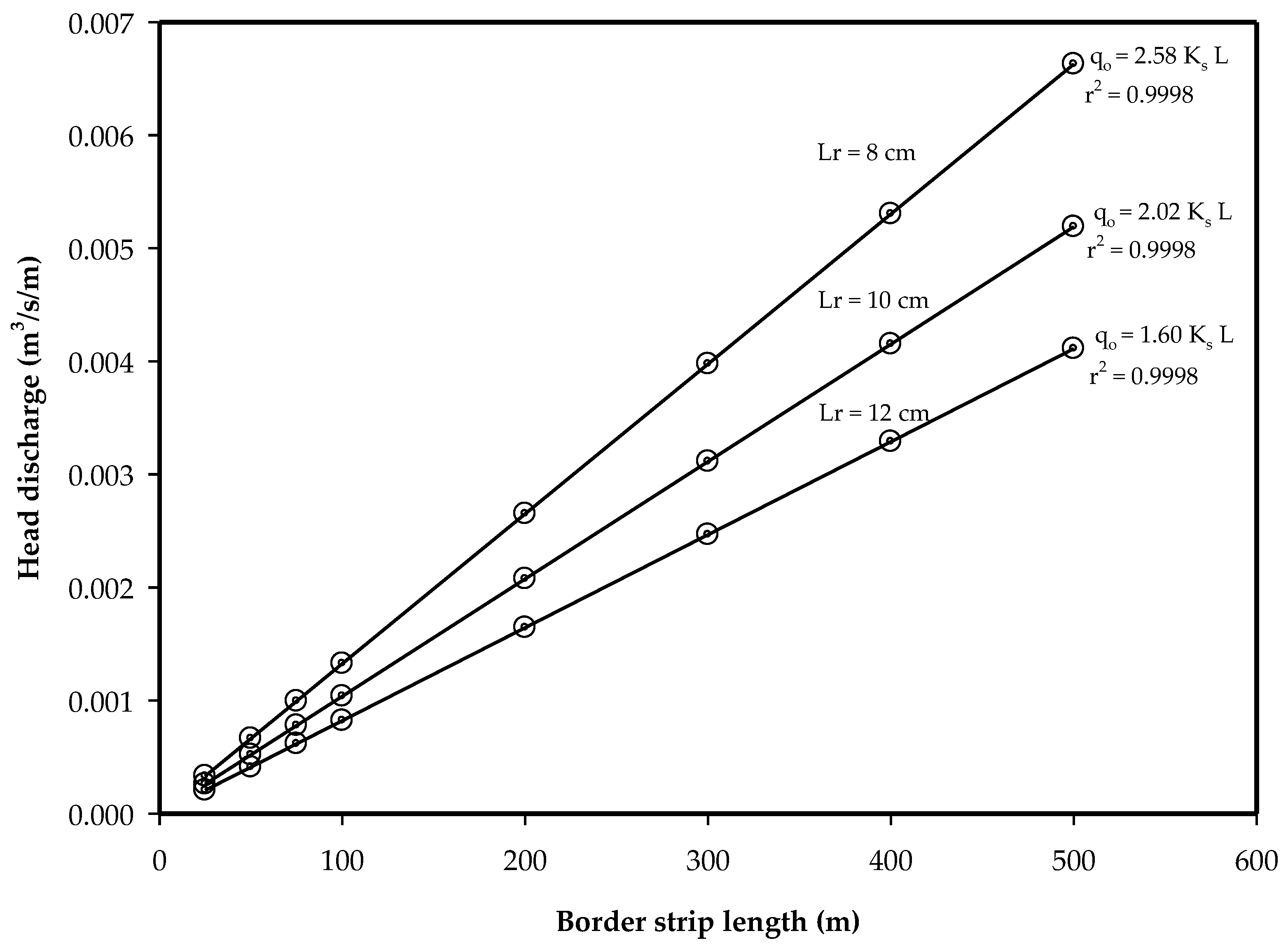
The numerical simulation of the irrigation with the system of Barre de Saint-Venant and Richards equations indicates that the relationship between optimal flow () and length (L) is approximately linear, for a soil type, topographic slope, friction coefficient, and irrigation depth, that is:
where qu has units of unitary flow per length unit. In addition, as qu is a constant, it follows that for the application of a specific irrigation depth, there is an irrigation time, unique and independent of the length, which allows obtaining a maximum value of the uniformity coefficient.
The relation (12) is illustrated by Saucedo et al. [27] in the loam soil of the experimental field of the Colegio de Postgraduados, Montecillo, State of Mexico, for water depths of 8, 10, and 12 cm, by making qu = αuKs, where αu is a dimensionless parameter (Figure 1). It is observed that there is monotony in the sense that the slope of the relationship between the border length and optimal flow decreases as the irrigation depth increases.
3.1.4. Irrigation Design Table
To generate the design table, it was necessary to obtain the relationships between optimal flow and border length for various soil types. The moisture content of residual water (θr) was assumed to be zero, according to Fuentes et al. [34]. The moisture content at saturation (θs) was assimilated to the total soil porosity (ϕ) determined, as the hydraulic conductivity at saturation (Ks), starting from the soil texture according to the relationships provided by Rawls and Brakensiek [41].
To estimate the value of the shape m parameter of the soil retention curve, one granulometric curve was reconstructed for each soil based on the percentages of sand, silt, and clay present in the triangle of textures [34]; we have followed the procedure suggested by Fuentes [38] to determine the values of m and η. The pressure scale (ψd) was determined from the suction of the wetting front of Green and Ampt equation [31] according to the texture and porosity of soils [41], as this suction was identified with the Bouwer scale [42] defined by:
where K0 = K(ψ0) is the hydraulic conductivity corresponding to the initial pressure ψ0 = ψ(θ0) related to the initial moisture content θ0, D(θ) = K(θ) dψ/dθ is the hydraulic diffusivity.
The parameter ψd is deduced by introducing the hydrodynamic characteristics defined by Equations (4) and (5) in Equation (13), considering the initial moisture content equal to the residual moisture content (ψ0 ∞), as follows:
where B(p,q) = Γ(p)Γ(q)/Γ(p + q) is the complete beta function, with p > 0 and q > 0, and Γ(x) the Euler complete gamma function.
The parameter values of the hydrodynamic characteristics are shown in Table 1 for different types of soil [27], where the residual moisture content is θr = 0 cm3/cm3.
The initial moisture content is considered as that which corresponds when the available moisture of each soil type has been consumed in a certain fraction. The available soil moisture is defined as the difference between the moisture contents at field capacity (θCC) and permanent wilting point (θPMP), whose values for each type of soil are estimated according to the soil texture triangle [41]. The initial moisture content is calculated as:
where Fap is the permissible depletion factor of the crop. The average value of 0.5 has been assumed. The values of initial moisture content are reported in Table 2.
As for the parameters of the law of resistance defined by Equation (8), the values were taken from a loam soil border in the Montecillo experimental field. Considering the Reynolds number, the regime is depth, d = 1, the value k = 1/54 is obtained thus that the advance curve provided by the numerical solution describes the advance curve observed in an irrigation test; the coefficient of kinematic viscosity is taken as ν = 10−6 m2/s. The longitudinal topographical slope of the border is of J0 = 0.002 m/m, value that is used to simulate irrigation in other borders with different soil types. With the hydrodynamic characterization of soils and θ0, the constant involved in the relationship between the border length and the optimal flow for a given irrigation depth is calculated.
The value of the constant is expressed in terms of flow per unit area, i.e., per unit width, and per unit length of border, results are shown in Table 3. The same table shows the irrigation time (τb) obtained at the moment the flow supply is cut off when the volume of irrigation per width unit is already stored both on the surface as well as inside the soil. In Rendón et al. [39], a table of similar design to Table 3 is shown containing some inconsistencies of monotony between the relationship that the variables optimal flow, irrigation time, and applied depth since the used model has difficulties in reproducing gravity irrigation in relatively long times. The coupling of Saint-Venant and Richards equations allows obtaining results that keep the monotony in the design variables, as shown in Table 3.
3.2. Analytical Representation of the Relationship between the Optimal Flow and Length
Equation (12) structure is deduced considering that the net water volume per width unit of the border is equal to the product of the border length (L) by the net irrigation depth (ℓn) and is also equal to the product of supply unitary flow (qo) by the time necessary to infiltrate the net depth (τn): qoτn = Lℓn. The relationship is also attested by involving the irrigation time to obtain the volume per width unit provided by the gross depth: qo τb = Lℓb. Comparing both results to Equation (12), we have:
It should be noted that this relationship involves, considering Equation (9), the following expression for application efficiency:
From the continuity equation, it can be shown that the unitary flow of minimal irrigation thus that the water wave arrives at the end of the channel is given by qm = Ks L; then it follows that the optimal flow must meet the inequality qo ≥ qm. If qo = αu qm is written, αu is a dimensionless parameter that must satisfy αu ≥ 1. Equations (12) and (16) should be written as follows:
in which the dependence of αu should be investigated regarding the irrigation depth and soil properties.
The extreme behavior of αu is deduced from the extreme behavior of the infiltrated depth. In very short times I = S [43], where S is sorptivity, and, therefore, τn = /S2, that is αu = S2/(Ks ℓn). In long times I~Io + Ks t, where Io is the ordinate at the origin depending on S and Ks, and on the Green and Ampt model on the time logarithm, and, therefore, αu~ℓn/(ℓn − Io). From the above, it follows that the limits:
must be satisfied by the general function αu (ℓn).
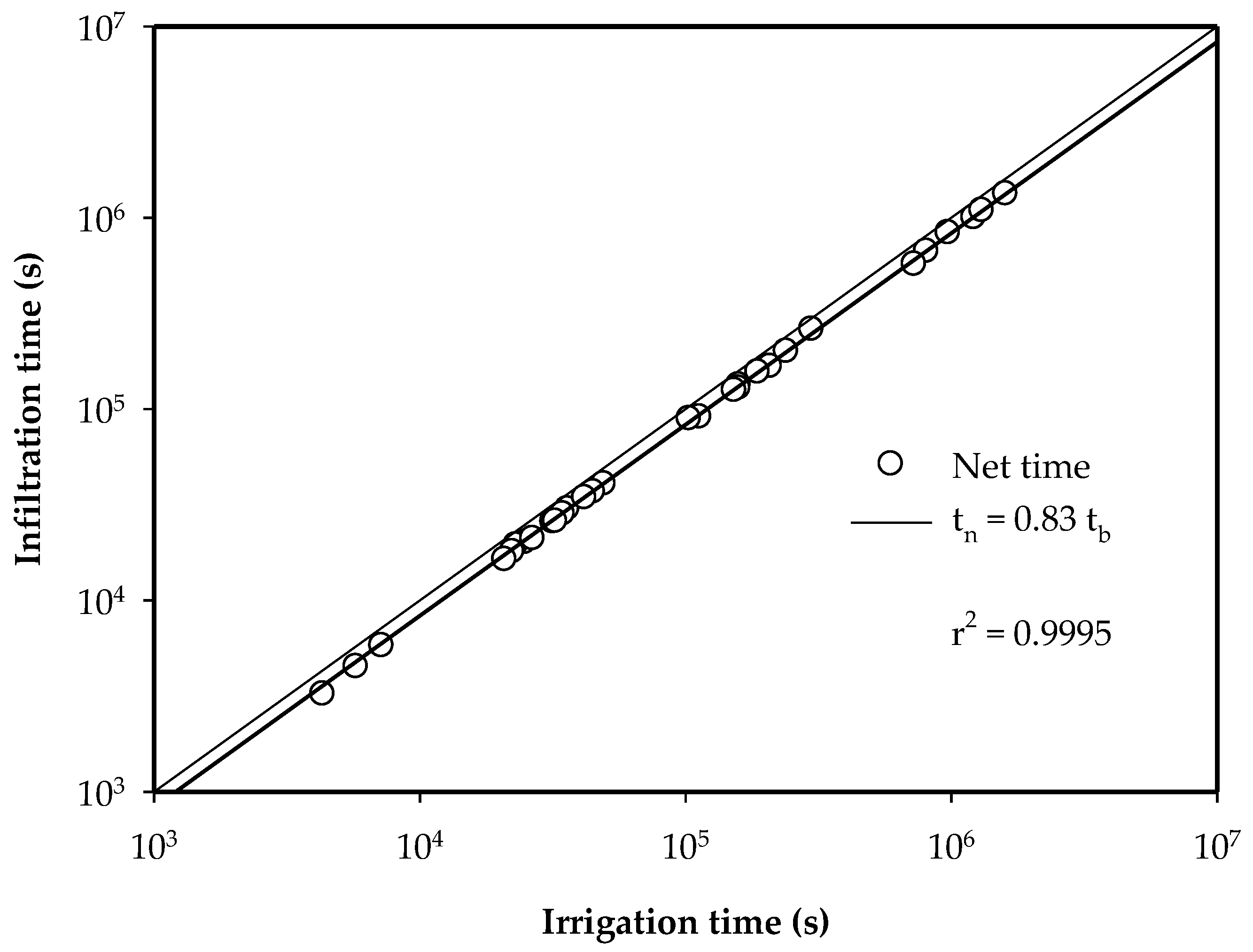
Irrigation time (τb) shown in Table 3 corresponds to the gross irrigation depth and is greater than the infiltration time corresponding to the net depth calculated from Equation (16): τn = ℓn/qu. Figure 2 shows the relationship between the two times; one has τn ≈ 0.83 τb with r2 = 0.9995, which indicates that, according to Equation (17), the average application efficiency with the optimal flow is ηA ≈ 83% for analyzed soils.
The design table can be represented algebraically if the infiltration function is provided analytically. This is obtained from the Parlange et al. model [44] deduced from the Richards equation, assuming that the hydraulic diffusivity tends to behave like a Dirac density and form a relationship between the hydraulic diffusivity and hydraulic conductivity. The model with the effect of water depth on the soil surface is as follows [30]:
where ∆θ = θs − θ0 is the storage capacity of the soil, h is the water depth on the soil surface, S is the sorptivity, and β is a shape parameter thus that 0 < β < 1, the lower limit corresponds to the Green and Ampt model while the higher limit corresponds to the Talsma and Parlange model [45]. Time in Equation (20) should be interpreted as the contact time that water has at a given point of the border.
Sorptivity S can be calculated with the expression proposed by Parlange [46]:
and the parameter of β shape can be calculated with the expression proposed by Fuentes [47]:
Variation in time of water depth on the soil is provided by the system of Saint-Venant and Richards equations, but their analytical representation is not known, the reason whereby it is assumed that it is represented by an average value; the mean depth of water can be estimated as a fraction of the normal depth: = hn. With the dimensionless variables:
Equation (20) is written as:
The relationship dI*/d = dt*/d, considering constant the water depth on the surface, along with the initial condition t* = 0, I* = 0, ∞, leads to find the time as a function of the infiltration flow:
Thus, the function defining the infiltrated depth in the function of time is of a parametric nature: I* = I* () and t* = t* (), with the flow as a parameter.
Due to the high nonlinearity of the function K(θ) it can be assumed that K0 << Ks. The dimensionless version of αu defined in Equation (18) is as follows:
where the dimensionless net irrigation time and net irrigation depth are defined by Equation (23) and the corresponding dimensionless infiltration flow by Equation (24). For a given border and initial medium depth, the irrigation depth in a dimensionless form () was calculated, and the dimensionless flow () was calculated with Equation (25) iteratively. Finally, the dimensionless net time () was calculated with Equation (26), and αu was calculated with Equation (27).
It should be noted that the process of calculating the optimal flow, for a given irrigation length, was also iterative since the medium depth depended on the normal depth and this, in turn, of the optimal flow, through Equation (8): hn = [ν2 (qo/kν)1/d/gJo]1/3.
When the water depth was small ( << S2/2Ks∆θ) from Equation (25) it was deduced an explicit function of time with respect to the infiltrated water and corresponds to the Parlange et al. equation [44]:
In Table 4, the values of sorptivity and the shape parameter for different soils are reported. In Figure 3, the optimal infiltration time obtained with Saint-Venant and Richards equations is compared with that obtained with Equation (28) of Parlange et al. [44]: r2 = 0.9866.
The shape parameter β varies with respect to the initial moisture content; however, it does not vary significantly when this moisture content approaches the residual moisture content. In this case the introduction of the hydrodynamic characteristics defined by Equations (4) and (5) in Equation (22) provides:
where B(p,q) is the complete beta function.
Introduction of Equation (28) into Equation (27) gives the approximate formula for calculating the optimal unitary flow in function of the border length, the net depth, and the characteristic parameters of infiltration representing the capillary forces (sorptivity) and gravitational forces (hydraulic conductivity at saturation) and a shape parameter of the hydrodynamic characteristics, namely:
where is the net irrigation depth in dimensionless writing.
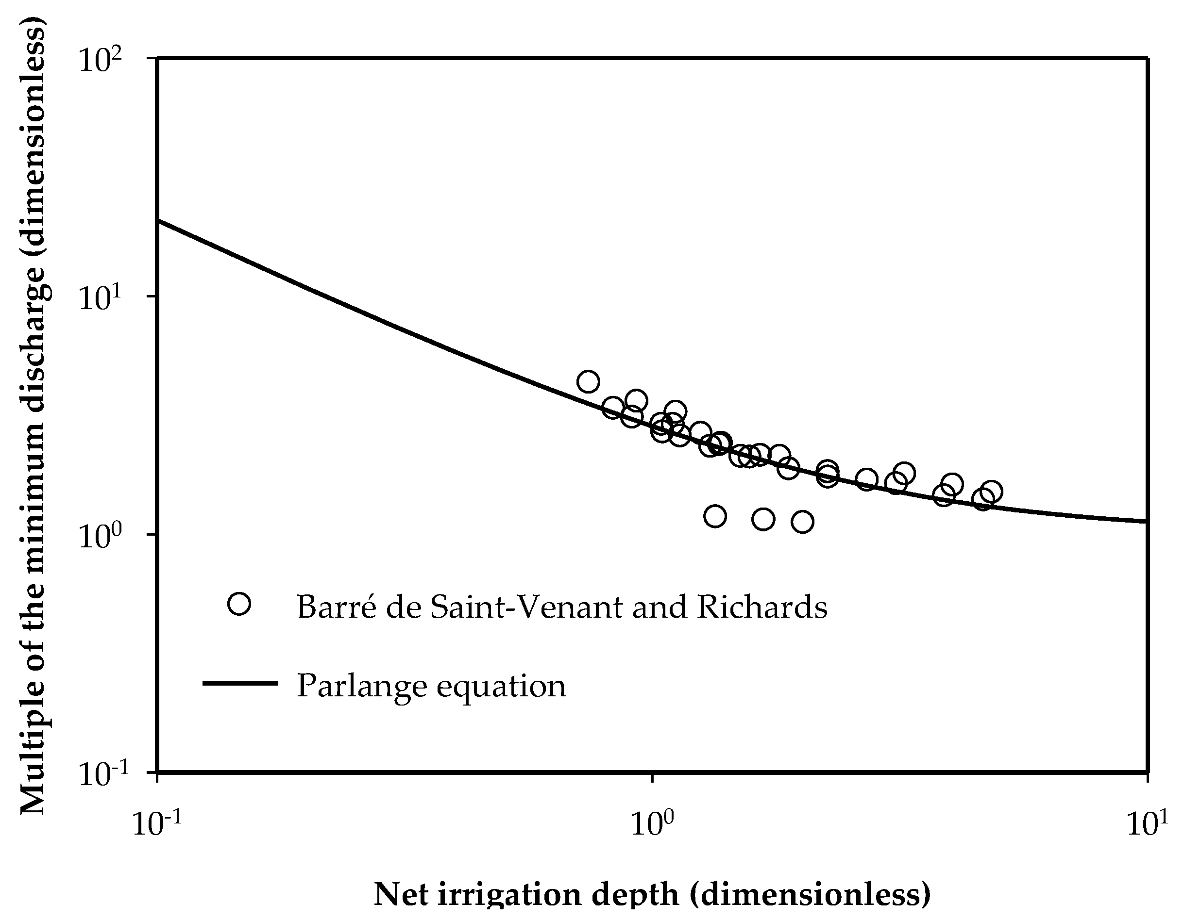
As can be seen, Equation (30) contains a shape parameter in the function of the soil type; however, it does not have a great variation in the range of soils reported in Table 4, the mean value β ≈ 3/4 can be taken. With this value in Figure 4, the graph of Equation (30) and its comparison with the numerical results are presented. A good agreement is clearly demonstrated.
3.3. Application of the Analytical Formula in Furrow Irrigation Systems
This analytical formula has been applied in field experiments realized by Chávez and Fuentes [1] with good results. Irrigation tests (250) were performed in 1010 ha with the next crops: Zea mayz, Sorghum vulgare, Medicago sativa, Phaseolus vulgaris, Pachyrhizus erosus, Hordeum vulgare, Triticum aestivum, and Allium cepa.
The characteristics and properties that were measured in the plots were: Length, slope, texture, bulk density, initial, and saturation moisture content. The results that were obtained from the evaluation of the irrigation tests were: Discharge at the entrance of the plot, number of furrows by irrigation set, saturated hydraulic conductivity, the efficiency of the application, and the slope of the direction of irrigation. The irrigation tests were performed in plots.
With the advanced and recession data and the characteristics of the soils from the locations where the irrigation tests were carried out, the calibration of the test was performed using the kinematic wave model. With the parameters found (Ks and hf) for the evaluation of the irrigation tests and the net irrigation depth that is intended to be applied on the plot (water depth depending on each of the crops established in the plots), Equations (18) and (30) were used to make the design. The obtained result is the optimal flow that must go into each furrow; for this value, the discharge for the entrance of the plot between that obtained with Equation (18) was divided, and then approached the nearest whole value. As a result, the equation gives us the number of furrows that the user has to open by set and the time that must pass before cutting off the water.
In this study, the evaluation of irrigation tests, the data of the plot, and the net irrigation depth to be applied demonstrated that the optimal flow expense that can be put in each furrow during an irrigation event can be calculated under the hypothesis that with this expense, the historical water depths applied in the evaluated plots can be reduced. The average water depths decreased by 19 cm, irrigation time decreased 12 h ha−1 on average, and the average volume saved was 2150 m3 ha−1, which represented a total of 49% of the total volume used. In addition, the average efficiency rose from 51% to 86%.
4. Conclusions
A linear relationship has been validated between the length of the border and the optimal irrigation flow, defined as the inflow rate that has to be applied to obtain a maximum value of Christiansen’s uniformity coefficient with high values of application efficiency and irrigation requirement efficiency. The linear form of the proportion between both variables was corroborated by [39] using a hydrological model for the flow of surface water and the Green and Ampt infiltration equation.
The proportion between optimal flow and border length has been established by numerical simulation with the hydrodynamic model, formed by the coupled equations of Barré de Saint-Venant and Richards. In the numerical simulation, 10 types of soils of contrasting texture have been used and three water depths applied, which has allowed us to form an irrigation design table, that is, 10 linear relationships for each irrigation depth.
To establish an analytical representation of the optimal flow in function of the border length, the Parlange infiltration theory proposed for integrating the differential equation of the vertical one-dimensional infiltration has been used. In the formula obtained to relate the optimal irrigation flow and length, the irrigation depth intervenes and as soil parameters sorptivity that comes from the capillary forces and the saturated hydraulic conductivity that comes from gravitational forces. The good accordance between the results of numerical simulation and analytical representation allows us to obtain the formula for the design of gravity irrigation.
Author Contributions
Conceptualization, C.F.; methodology, C.F. and C.C.; software, C.F.; validation, C.C. and C.F.; formal analysis, C.C.; investigation, C.F.; resources, C.F. and C.C.; data curation, C.F. and C.C.; writing—original draft preparation, C.F.; writing—review and editing, C.C.; visualization, C.F. and C.C.; supervision, C.F.; project administration, C.F. and C.C.; funding acquisition, C.F. All authors have read and agreed to the published version of the manuscript.
Funding
This research received no external funding.
Conflicts of Interest
The authors declare no conflict of interest.
References
- Chávez, C.; Fuentes, C. Design and evaluation of surface irrigation systems applying an analytical formula in the irrigation district 085, La Begoña, Mexico. Agric. Water Manag. 2019, 221, 279–285. [Google Scholar] [CrossRef]
- Fuentes, C.; De León, B.; Saucedo, H.; Parlange, J.-Y.; Antonino, A.C.D. Saint-Venant and Richards equations system in surface irrigation: (1) Hydraulic resistance power law. Ing. Hidraul. Mexico 2004, 19, 65–75. [Google Scholar]
- Khanna, M.; Malano, H.M. Modelling of basin irrigation systems: A review. Agric. Water Manag. 2006, 83, 87–99. [Google Scholar] [CrossRef]
- Soroush, F.; Fenton, J.D.; Mostafazadeh-Fard, B.; Mousavui, S.F.; Abbasi, F. Simulation of furrow irrigation using the Slow-change/slow-flow equation. Agric. Water Manag. 2013, 116, 160–174. [Google Scholar] [CrossRef]
- Ebrahimian, H.; Liaghat, A. Field Evaluation of Various Mathematical Models for Furrow and Border Irrigation Systems. Soil Water Res. 2011, 2, 91–101. [Google Scholar] [CrossRef] [Green Version]
- Furman, A.; Warrick, A.W.; Zerihun, D.; Sanchez, D.A. Modified Kostiakov infiltration function: Accounting for initial and boundary conditions. J. Irrig. Drain. Eng. 2006, 132, 587–597. [Google Scholar] [CrossRef]
- Parhi, P.K.; Mishra, S.K.; Singh, R. A modification to Kostiakov and modified Kostiakov infiltra-tion models. Water Resour. Manag. 2007, 21, 1973–1989. [Google Scholar] [CrossRef]
- Zhang, S.; Xu, D.; Li, Y. A one-dimensional complete hydrodynamic model of border irrigation based on a hybrid numerical method. Irrig. Sci. 2011, 29, 93–102. [Google Scholar] [CrossRef] [Green Version]
- Strelkoff, T.; Katopodes, N. Border-irrigation hydraulics with zero inertia. J. Irrig. Drain. Div. ASCE 1977, 102, 325–342. [Google Scholar]
- Bautista, E.; Wallender, W.W. Hydrodynamic furrow irrigation model with especified space steps. J. Irrig. Drain. Eng. Div. ASCE 1992, 118, 450–465. [Google Scholar] [CrossRef]
- Sohrabi, B.; Behnia, A. Evaluation of Kostiakov´s infiltration equation in furrow irrigation design according to FAO Method. J. Agron. 2007, 6, 468–471. [Google Scholar]
- Bautista, E.; Clemmens, A.J.; Strelkoff, T.S.; Schlegel, J. Modern analysis of surface irrigation systems with WinSRFR. Agric. Water Manag. 2009, 96, 1146–1154. [Google Scholar] [CrossRef]
- Strelkoff, T.; Clemmens, A.J. Hydraulics of surface systems. In Design and Operation of Farm Irrigation Systems, 2nd ed.; Hoffman, G.J., Evans, R.G., Jensen, M.E., Martin, D.L., Elliot, R.L., Eds.; ASABE: St. Joseph, MO, USA, 2007; pp. 436–498. [Google Scholar]
- Gillies, M.H.; Smith, R.J. SISCO: Surface irrigation simulation, calibration and optimisation. Irrig. Sci. 2015, 33, 339–355. [Google Scholar] [CrossRef]
- Valipour, M. Comparison of surface irrigation simulation models: Full hydrodynamic, zero inertia, kinematic wave. J. Agric. Sci. 2012, 4, 68–74. [Google Scholar] [CrossRef]
- Mahdizadeh, K.M.; Gholami, S.M.A.; Valipour, M. Simulation of open- and closed-end border irrigation systems using SIRMOD. Arch. Agron. Soil Sci. 2015, 61, 929–941. [Google Scholar] [CrossRef]
- Salahou, M.K.; Jiao, X.; Lü, H. Border irrigation performance with distance-based cut-off. Agric. Water Manag. 2018, 201, 27–37. [Google Scholar] [CrossRef]
- Akbari, M.; Gheysari, M.; Mostafazadeh-Fard, B.; Shayannejad, M. Surface, irrigation simulation-optimization model based on meta-heuristic algorithms. Agric. Water Manag. 2018, 201, 46–57. [Google Scholar] [CrossRef]
- Lalehzari, R.; Nasab, S.B. Improved volume balance using upstream flow depth for advance time estimation. Agric. Water Manag. 2017, 186, 120–126. [Google Scholar] [CrossRef]
- Liu, K.H.; Jiao, X.Y.; Li, J.; An, Y.H.; Guo, W.H.; Salahou, M.K.; Sang, H. Performance of a zero-inertia model for irrigation with rapidly varied inflow discharges. Int. J. Agric. Biol. Eng. 2020, 13, 175–181. [Google Scholar]
- Moravejalahkami, B.; Mostafazadeh-Fard, B.; Heidarpour, M.; Abbasi, F. Research Paper: SW-Soil and Water Furrow infiltration and roughness prediction for different furrow inflow hydrographs using a zero-inertia model with a multilevel calibration approach. Biol. Eng. 2009, 103, 374–381. [Google Scholar]
- González, C.J.M.; Muñoz, H.B.; Acosta, H.R.; Mailhol, J.C. Kinematic wave model adapted to irrigation with closed-end furrows. Agrociencia 2006, 40, 731–740. [Google Scholar]
- Rendón, P.L.; Saucedo, H.; Fuentes, C. Diseño del Riego por Gravedad, 1st ed.; Fuentes, C., Rendón, L., Eds.; Universidad Autónoma de Querétaro: Santiago de Querétaro, Mexico, 2012; pp. 321–358. [Google Scholar]
- Richards, L.A. Capillary conduction of liquids through porous mediums. Physics 1931, 1, 318–333. [Google Scholar] [CrossRef]
- Saucedo, H.; Fuentes, C.; Zavala, M. The Saint-Venant and Richards equation system in surface irrigation: (2) Numerical coupling for the advance phase in border irrigation. Ing. Hidraul. Mexico 2005, 20, 109–119. [Google Scholar]
- Saucedo, H.; Zavala, M.; Fuentes, C. Complete hydrodynamic model for border irrigation. Water Technol. Sci. 2011, 2, 23–38. [Google Scholar]
- Saucedo, H.; Zavala, M.; Fuentes, C.; Castanedo, V. Optimal flow model for plot irrigation. Water Technol. Sci. 2013, 4, 135–148. [Google Scholar]
- Castanedo, V.; Saucedo, H.; Fuentes, C. Comparison between a hydrodynamic full model and a hydrologic model in border irrigation. Agrociencia 2013, 47, 209–223. [Google Scholar]
- Schmitz, G.; Haverkamp, R.; Palacios, O. A coupled surface-subsurface modelor shallow water flow over initially dry-soil. In Proceedings of the 21st Congress (IAHR), Melbourne, Australia, 13–18 August 1985; Volume 1, pp. 23–30. [Google Scholar]
- Parlange, J.-Y.; Haverkamp, R.; Touma, J. Infiltration under ponded conditions. Part I. Optimal analytical solutions and comparisions with experimental observations. Soil Sci. 1985, 139, 305–311. [Google Scholar] [CrossRef]
- Green, W.H.; Ampt, G.A. Studies in soil physics, I: The flow of air and water through soils. J. Agric. Sci. 1911, 4, 1–24. [Google Scholar]
- Vázquez, F. Eficiencia de aplicación en el riego con surcos cerrados al existir dos pendientes. Ing. Investig. Tecnol. 2000, 3, 123–130. [Google Scholar]
- Darcy, H. Dètermination des lois d’ècoulement de l’eau à travers le sable. In Les Fontaines Publiques de la Ville de Dijon; Victor Dalmont: Paris, France, 1856; pp. 590–594. [Google Scholar]
- Fuentes, C.; Haverkamp, R.; Parlange, J.-Y. Parameter constraints on closed–form soil-water relationships. J. Hydrol. 1992, 134, 117–142. [Google Scholar] [CrossRef]
- Van Genuchten, M.T. A closed-form equation for predicting the hydraulic conductivity of unsaturated soils. Soil Sci. Soc. Am. J. 1980, 44, 892–898. [Google Scholar] [CrossRef] [Green Version]
- Burdine, N.T. Relative permeability calculation from size distributions data. Trans. AIME 1953, 198, 171–199. [Google Scholar] [CrossRef]
- Brooks, R.H.; Corey, A.T. Hydraulic properties of porous media. Hydrol. Pap. (Colo. State Univ.) 1964, 3, 27. [Google Scholar]
- Fuentes, C. Approche Fractale des Transferts Hydriques Dans les sols non Saturès. Ph.D. Thesis, Universidad Joseph Fourier de Grenoble, Francia, France, 1992; p. 267. [Google Scholar]
- Rendón, P.L.; Saucedo, H.; Fuentes, C. Gravity Irrigation Design. In Gravity Irrigation, 1st ed.; Fuentes, C., Rendón, L., Eds.; National Association of Irrigation Specialist: Mexico, Mexico, 2017; pp. 345–386. [Google Scholar]
- Lewis, M.R.; Milne, W.E. Analysis of border irrigation. Agric. Eng. 1938, 19, 267–272. [Google Scholar]
- Rawls, W.J.; Brakensiek, D.L. Estimating soil water retention from soil properties. Am. Soc. Civ. Eng. 1981, 108, 167–171. [Google Scholar]
- Bouwer, H. Rapid field measurement of air entry value and hydraulic conductivity of soil as significant parameters in flow system analysis. Water Resour. Res. 1964, 36, 411–424. [Google Scholar] [CrossRef]
- Philip, J.R. The theory of infiltration: 1. The infiltration equation and its solutions. Soil Sci. 1957, 83, 345–357. [Google Scholar] [CrossRef]
- Parlange, J.-Y.; Braddock, R.D.; Lisle, I.; Smith, R.E. Three parameter infiltration equation. Soil Sci. 1982, 111, 170–174. [Google Scholar] [CrossRef]
- Talsma, T.; Parlange, J.-Y. One-dimensional vertical infiltration. Aust. J. Soil. Res. 1972, 10, 143–150. [Google Scholar] [CrossRef]
- Parlange, J.-Y. On solving the flow equation in unsaturated soils by optimization: Horizontal infiltration. Soil Sci. Soc. Am. Proc. 1975, 39, 415–418. [Google Scholar] [CrossRef]
- Fuentes, C. Teoría de la infiltración unidimensional: 2. La infiltración vertical. Agrociencia 1989, 78, 119–153. [Google Scholar]
Figure 1.
Relationship between the border strip length and the optimum input discharge in the loam soil of Montecillo for three irrigation depths: 8, 10, and 12 cm. Ks in m/s.
Figure 1.
Relationship between the border strip length and the optimum input discharge in the loam soil of Montecillo for three irrigation depths: 8, 10, and 12 cm. Ks in m/s.

Figure 2.
Relationship between the irrigation time of the gross depth (ℓb) and the infiltration time of the net depth (ℓn).
Figure 2.
Relationship between the irrigation time of the gross depth (ℓb) and the infiltration time of the net depth (ℓn).

Figure 3.
Comparison between the optimal irrigation time numerically obtained with the Barré de Saint-Venant/Richards equations and those calculated ones with the Parlange et al. equation (Equation (28)).
Figure 3.
Comparison between the optimal irrigation time numerically obtained with the Barré de Saint-Venant/Richards equations and those calculated ones with the Parlange et al. equation (Equation (28)).

Figure 4.
The multiple factors of the minimum discharge as a function of the irrigation depth numerically obtained with the Saint-Venant and Richards equations, and those calculated with the Parlange et al. model [44], Equation (30).
Figure 4.
The multiple factors of the minimum discharge as a function of the irrigation depth numerically obtained with the Saint-Venant and Richards equations, and those calculated with the Parlange et al. model [44], Equation (30).


Table 1.
Hydrodynamic characteristics of soils for irrigation design by borders.
| Soil Texture | θs (cm3/cm3) | λc (cm) | Ks (cm/h) | η | m | |ψd| (cm) |
|---|---|---|---|---|---|---|
| Clay | 0.525 | 140.26 | 0.010 | 61.10 | 0.0229 | 132.50 |
| Silty clay | 0.500 | 100.16 | 0.015 | 31.55 | 0.0440 | 94.70 |
| Silty-clay-loam | 0.500 | 60.12 | 0.070 | 15.34 | 0.0905 | 57.80 |
| Clay-loam | 0.475 | 36.00 | 0.150 | 19.30 | 0.0714 | 34.15 |
| Sandy clay | 0.425 | 25.72 | 0.200 | 41.50 | 0.0327 | 23.70 |
| Loam | 0.500 | 30.52 | 0.500 | 5.61 | 0.2477 | 30.70 |
| Silt | 0.475 | 20.04 | 0.700 | 13.93 | 0.0989 | 19.20 |
| Silty loam | 0.525 | 30.07 | 0.600 | 12.01 | 0.1165 | 29.35 |
| Sandy-clay-loam | 0.425 | 35.61 | 1.500 | 18.44 | 0.0736 | 33.35 |
| Sandy loam | 0.450 | 10.00 | 5.000 | 13.62 | 0.1004 | 9.52 |
Table 2.
Moisture constants.
| Soil Texture | θPMP (cm3/cm3) | θCC (cm3/cm3) | θ0 (cm3/cm3) |
|---|---|---|---|
| Clay | 0.350 | 0.450 | 0.400 |
| Silty clay | 0.275 | 0.425 | 0.350 |
| Silty clay-loam | 0.200 | 0.375 | 0.287 |
| Clay-loam | 0.190 | 0.340 | 0.265 |
| Sandy clay | 0.225 | 0.325 | 0.275 |
| Loam | 0.100 | 0.275 | 0.187 |
| Silt | 0.130 | 0.250 | 0.190 |
| Silt loam | 0.125 | 0.275 | 0.200 |
| Sandy-clay-loam | 0.150 | 0.250 | 0.200 |
| Sandy loam | 0.100 | 0.190 | 0.145 |
Table 3.
Table of the border irrigation design: flow in l/s/m2 for the optimal application of the irrigation depth.
Table 3.
Table of the border irrigation design: flow in l/s/m2 for the optimal application of the irrigation depth.
| Soil Texture | ℓn = 8 cm | ℓn = 10 cm | ℓn = 12 cm | |||
|---|---|---|---|---|---|---|
| qu (l/s/m2) | τb (h) | qu (l/s/m2) | τb (h) | qu (l/s/m2) | τb (h) | |
| Clay | 0.00012 | 224.1 | 0.00010 | 338.2 | 0.00009 | 445.0 |
| Silty clay | 0.00014 | 201.6 | 0.00012 | 270.5 | 0.00011 | 362.5 |
| Silty-clay-loam | 0.00060 | 44.1 | 0.00050 | 66.6 | 0.00046 | 82.9 |
| Clay-loam | 0.00088 | 31.4 | 0.00078 | 44.0 | 0.00072 | 57.8 |
| Sandy clay | 0.00090 | 28.7 | 0.00080 | 42.4 | 0.00077 | 52.0 |
| Loam | 0.00399 | 6.9 | 0.00333 | 10.0 | 0.00296 | 13.7 |
| Silt | 0.00411 | 6.4 | 0.00354 | 9.6 | 0.00326 | 12.5 |
| Silt-loam | 0.00446 | 6.2 | 0.00388 | 8.8 | 0.00349 | 11.6 |
| Sandy-Clay-loam | 0.00490 | 5.8 | 0.00476 | 7.4 | 0.00464 | 9.0 |
| Sandy-loam | 0.02476 | 1.2 | 0.02223 | 1.6 | 0.02073 | 2.0 |
Table 4.
Parameters of the Parlange et al. infiltration equation [44]: sorptivity (S) and the shape parameter (β), calculated with Equations (21) and (29).
Table 4.
Parameters of the Parlange et al. infiltration equation [44]: sorptivity (S) and the shape parameter (β), calculated with Equations (21) and (29).
| Soil Texture | S (cm/) | β | Soil Texture | S (cm/) | β |
|---|---|---|---|---|---|
| Clay | 0.583 | 0.820 | Loam | 2.958 | 0.584 |
| Silty clay | 0.655 | 0.800 | Silt | 2.761 | 0.744 |
| Silty-clay-loam | 1.296 | 0.750 | Silty loam | 3.338 | 0.721 |
| Clay loam | 1.469 | 0.773 | Sandy-clay-loam | 4.796 | 0.775 |
| Sandy clay | 1.223 | 0.820 | Sandy loam | 5.404 | 0.744 |
© 2020 by the authors. Licensee MDPI, Basel, Switzerland. This article is an open access article distributed under the terms and conditions of the Creative Commons Attribution (CC BY) license (http://creativecommons.org/licenses/by/4.0/).
Share and Cite
MDPI and ACS Style
Fuentes, C.; Chávez, C. Analytic Representation of the Optimal Flow for Gravity Irrigation. Water 2020, 12, 2710. https://doi.org/10.3390/w12102710
AMA Style
Fuentes C, Chávez C. Analytic Representation of the Optimal Flow for Gravity Irrigation. Water. 2020; 12(10):2710. https://doi.org/10.3390/w12102710
Chicago/Turabian StyleFuentes, Carlos, and Carlos Chávez. 2020. "Analytic Representation of the Optimal Flow for Gravity Irrigation" Water 12, no. 10: 2710. https://doi.org/10.3390/w12102710
Note that from the first issue of 2016, this journal uses article numbers instead of page numbers. See further details here.