Gravity-Induced Geometric Phases and Entanglement in Spinors and Neutrinos: Gravitational Zeeman Effect


Department of Physics, Indian Institute of Science, Bangalore 560012, India
*
Author to whom correspondence should be addressed.
Universe 2020, 6(10), 160; https://doi.org/10.3390/universe6100160
Submission received: 28 July 2020
/
Revised: 30 August 2020
/
Accepted: 23 September 2020
/
Published: 27 September 2020
(This article belongs to the Section Gravitation)
Abstract
:We show Zeeman-like splitting in the energy of spinors propagating in a background gravitational field, analogous to the spinors in an electromagnetic field, otherwise termed the Gravitational Zeeman Effect. These spinors are also found to acquire a geometric phase, in a similar way as they do in the presence of magnetic fields. However, in a gravitational background, the Aharonov-Bohm type effect, in addition to Berry-like phase, arises. Based on this result, we investigate geometric phases acquired by neutrinos propagating in a strong gravitational field. We also explore entanglement of neutrino states due to gravity, which could induce neutrino-antineutrino oscillation in the first place. We show that entangled states also acquire geometric phases which are determined by the relative strength between gravitational field and neutrino masses.
1. Introduction
It is well known that if the time dependence in the Hamiltonian arises through certain parameters, namely adiabatic parameters, then the system develops a non-dynamic phase, called the Berry phase [1]. Spinors propagating in the magnetic fields are known to acquire such a Berry phase. Interestingly, a neutrino propagating through a medium also develops such a system, while the varying matter density corresponds to the adiabatic parameter. Importantly, although originally Berry phase was found in the context of adiabatic, unitary and cyclic evolutions of time-dependent quantum systems, later it was re-established for non-adiabatic, non-unitary and non-cyclic cases with its generalized definition [2,3,4].
Several authors have studied the geometric phases in neutrino oscillations. Although it was argued in an earlier work that the Berry phase plays no role in two-flavor neutrino oscillations in matter [5], the work was restricted to a limited region in the parameter space. However, it was shown by exploiting the spin degree of freedom that the interaction of neutrinos with the transverse magnetic field can lead to a geometric effect [6,7,8,9]. Later on, it was argued [10] that the Berry phase can only appear in the presence of non-standard (e.g., R-parity violating supersymmetry) neutrino-matter interactions for the particular case of two-flavor oscillations in matter. Essentially, all of the above papers argued that geometric phases do not arise in the two-flavor neutrino oscillation probabilities with CP conservation in vacuum or in matter, in the absence of any non-standard neutrino-matter interactions. It was, however, furthermore argued [11] that even in the absence of CP violation, neutrinos in two-flavor oscillation in vacuum in a period can acquire an overall phase consisting of a dynamical phase and a phase depended on mixing angle only. The second part of the phase, which is of geometric origin, was called Berry phase. Note that this phase does not arise due to slowly varying parameters leading to adiabatic evolution, rather due to Schrödinger evolution of the system giving a closed loop in the Hilbert space. As the phase is a global phase at the amplitude level, it does not appear in measurable quantities like probabilities of appearance or survival of neutrinos. These cyclic geometric phases were furthermore extended by the later authors [12] to obtain non-cyclic phases for two- and three-flavor neutrinos in vacuum, which remain unobservable because of the same reason as before. Also, the geometric phases for neutrinos propagating in varying magnetic fields have been reported [13].
It is interesting to note that [14] the Berry phase has a connection to the phase discovered by Pancharatnam [15]. In fact, both of the phases can be described under the same platform [3]. Unlike the Berry phases obtained in the above work, it has however been established [16] that Pancharatnam phase can appear in detection probabilities and hence can be observed directly even in an effective two-flavor approximation. There are many other explorations over the years in various contexts of geometric phase and entanglement in neutrinos, including those with CPT violation and fluctuating matter, non-linear refraction, magnetic field, dissipative matter, etc. [17,18,19,20,21,22,23,24].
However, none of the works above considered the effects of gravity in the calculations, except one [24] which considered Newtonian self-gravitational interaction; whether the interaction of spinors and then neutrinos with gravitational field causes any effect or not. This issue particularly arises due to the fact that neutrinos interacting with background gravity may not preserve CPT [25,26], which may be shown as a natural candidate for governing the Berry phase, even in the evolution of neutrinos due to the split of dispersion energy between neutrino and antineutrino. Indeed, within the pure standard model of particle physics, the neutrino oscillations cannot be understood and hence relaxing the CPT conservation through gravitational interaction is one of the natural steps forward to beyond standard model. While the Berry phase arises in the presence of non-standard matter-neutrino interactions, neutrino spin and magnetic field interactions, it is a natural question if the coupling between spin of neutrino and in general spinor and spin connection to the background gravity generates any geometric effect.
Two-flavor neutrino oscillation in the background gravity has been discussed in various astrophysical contexts. One of the current authors explored possible Lorentz and CPT violations in the neutrino sector in the presence of background gravity and its astrophysical consequences [25,26,27,28,29]. Earlier, the analogy of solar neutrino oscillations with the precession of electron spin in a time-dependent magnetic field was discussed [30]. Then based on the evolution of a statistical ensemble, oscillations for neutrinos from supernovae or in the early universe in the presence of mixing and matter interactions in a thermal environment were shown to be viewed in terms of precession [31]. It was also observed [32] that spin flavor resonant transitions of neutrinos emanating from active galactic nuclei may occur in the vicinity of black holes due to gravitational effects and due to the presence of a large magnetic field. Interestingly, the matter effects therein become negligible in comparison to gravitational effects.
In the present paper, we start by recapitulating the origin of Berry phase in spinors in the presence of external magnetic fields in Section 2. Then we show the analogous effects in the presence of background gravitational fields, namely gravitational geometric phase in spinors in the same section. The subsequent plan is to apply this result in the neutrino sector. To do so, we first recapitulate the basic solutions of previous work discussing neutrino oscillations in curved spacetime [25,26] in Section 3, which are used in subsequent sections. Based on these neutrino states evolving in the gravitational background, we explore any geometric (as well as dynamic) effect/phase arising due to gravity in Section 4. Subsequently, our aim is to explore the possible entanglement of neutrino states coupled with background gravitational field and to compute the geometric phase arising in their evolution in Section 5. Finally, we discuss how the geometric phases actually vary with gravitational field in Section 6 and summarize results in Section 7.
2. Geometric Phases in the Presence of Electromagnetic and Gravitational Fields
2.1. In Electromagnetic Field
The Dirac equation, describing dynamics of spinors, in the presence of electromagnetic field and the underlying dispersion energy, Zeeman splitting and geometric/Berry phase are well-known. However, for the ease of understanding their similarities and also dissimilarities with those in the gravitational field, which is the main target here, we first recall the Dirac equation in the presence of electromagnetic field given by
where the various components of , where , are Dirac matrices with their usual meaning, e is the electric charge, m is the mass of the spinor and is the electromagnetic covariant 4-vector potential. Here, we choose units . For the non-trivial solution for , the energies/Hamiltonians of the spin-up and spin-down particles are given by
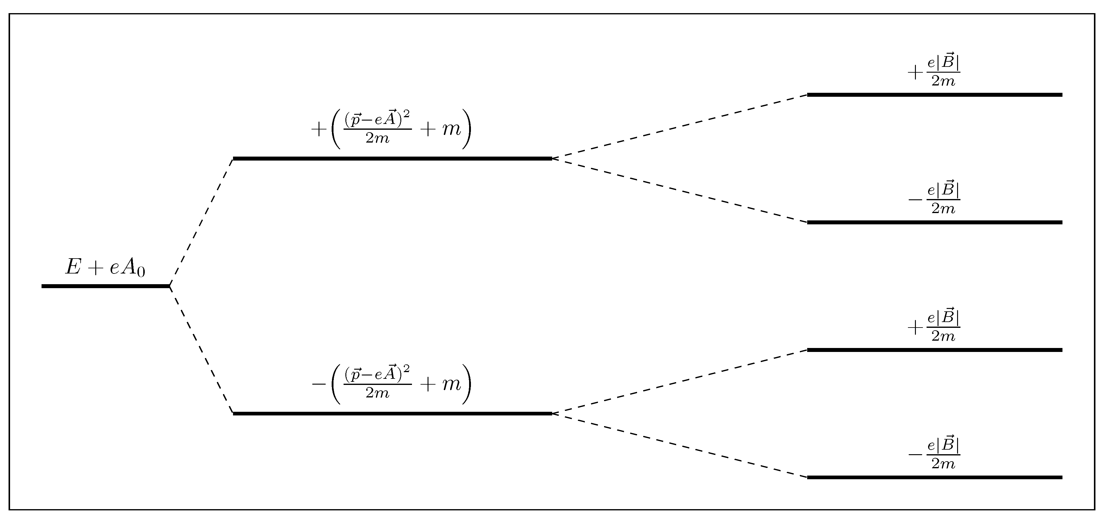
where is the temporal component of which is basically the Coulomb potential, is the quantum mechanical momentum operator , and is the Pauli spin matrix. In the non-relativistic limit, where is much larger than the rest of the terms in the R.H.S. of Equation (2), it reduces to
Apart from the split due to the positive and negative energy solutions, clearly there is an additional split in the respective energy levels. This is basically Zeeman-splitting governed by the term with Pauli’s spin matrix, in the up and down spinors for the positive and negative energy spinors induced by magnetic fields, whether we choose relativistic or non-relativistic regimes. The same governing term involved with is also responsible for the Berry phase if is varying. For convenience, is generally considered in the parameter space and is decomposed as . Hence, the Berry phase at a fixed r is given by
where , the coordinate vector of the underlying Poincaré sphere. When is constant, .
Figure 1 represents the energy splitting given by Equation (3). While the primary splitting corresponds to positive and negative energy solutions, the secondary splitting corresponds to the interaction between the spin and magnetic fields.
Recapitulation of all of the above results will be useful to explore and understand the consequences of the dynamics of spinors in the gravitational field. As we will show below, although there are certain similarities between the effects of electromagnetic and gravitational fields to the spinors, there are some unique consequences in the latter.
2.2. In Gravitational Field
Dirac equation in the presence of background gravitational fields has already been shown to have many consequences (see, e.g., the work by one of the present authors [25,26,28,33,34]) and is known to have the form (see, e.g., [26,34,35,36])
where is the gravitational covariant 4-vector potential (gravitational coupling with the spinor), given by
where -s and are various components of vierbeins and Christoffel connection with Greek and Latin indices respectively indicating curved and local flat coordinates, is the 4-dimensional Levi-Civita symbol and as usual. Here we do not repeat the calculation to obtain the reduced form of the Dirac equation given by Equation (5), which is available in the existing literature, see, e.g., [28,29,37] for details. The form of Equation (5) is easy to understand in local inertial coordinates, where the Dirac matrices and their relations are straight forward. However, it is not difficult to explore Dirac equation in general curvilinear coordinates (see, e.g., [38]). Nevertheless, in our first exploration of the geometric phase of spinors and neutrinos in gravitational background, for the convenience of developing the idea, we stick to the local inertial coordinates. This helps to compare results easily with geometric/Berry phase arising in the presence of magnetic field without losing any important physics. In the future, we will report geometric/Berry phase in gravitational field in global coordinates. Considering the problem in local coordinates, in brief, while expanding various terms of the Dirac Lagrangian (and equation) in curved spacetime, one obtains a Hermitian-like and anti-Hermitian-like parts, apart from the part already there in Minkowski spacetime. Hence, considering total Lagrangian consisting of that of particle and anti-particle (and corresponding equation), the anti-Hermitian part drops out and one obtains Equation (5) given above (see [37] for details). It can also be seen as the choice of an appropriate basis system [39], particularly clearer when we explore it in global non-inertial coordinates. Nevertheless, the appearance of the anti-Hermitian-like part (which need not always be anti-Hermitian, depending on the underlying spacetime) is independent of the Hermitian-like term [33] that alone could lead to the axial-vector term given by Equation (5), which is the basic building block of the following discussion. Hence, for simplicity, here we do not consider the apparent anti-Hermitian term.
Now, like the case of electromagnetic fields, for the non-trivial solution of in the spacetime not explicitly dependent on time (except the case where time dependence arises only via scale factor, like in an expanding universe, and the exploration is in a particular epoch or the interest is in the local-inertial coordinates), in the local coordinates, the energies/Hamiltonians of the spin-up and spin-down particles from Equation (5) are given by
where is the temporal component of and . In the regime of weak gravity and when is much larger than the rest of the terms in the R.H.S. of Equation (7), it reduces to
Equation (8) brings in a new effect due to the presence of an axial-vector term in the Dirac equation in the gravitational background as opposed to the case with electromagnetic effects involved with a vector term shown by Equation (3). The new effect induced by the axial-vector involves the spin–momentum coupling of the particle, apart from spin–gravity coupling, and other related terms, provided the background gravitational potential is non-zero. As in general gravitational potential is not constant (even if locally gravitational field is constant), the eigenfunction of Equation (8) cannot be plane-wave typed. However, if is slowly varying and time-independent, then the solution can be of the form
where is a slowly varying function. This leads the Hamiltonian to the form
As is determined by the variation of background gravitational potential, we can suitably choose in terms of and in such a way that the above Hamiltonian is Hermitian and terms involved with are removed, given by
where satisfies
Note that the solution for will turn out to be complex and its imaginary part may need to be adjusted by modifying of the solution. Obviously, this is one of the possible solutions and is a gauge choice, not unique. However, this will suffice for the present purpose when the aim is to show the existence of geometric phase and a possible new effect in gravitational background.
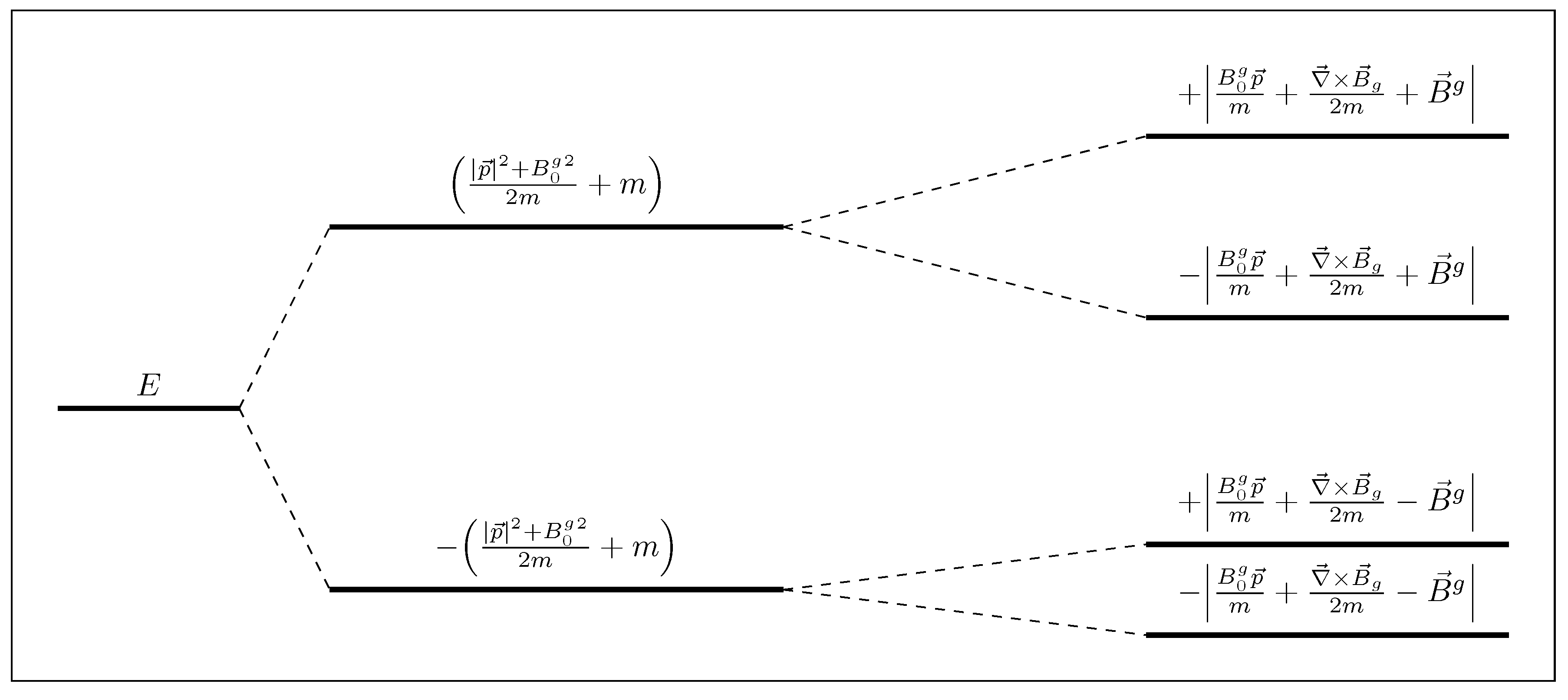
From Equation (11), there is a two-fold split in dispersion energy, governed by two terms associated with the Pauli spin matrix, between up and down spinors for the positive and negative energy spinors induced by gravitational fields, whether the field is weak or strong. The same governing terms are also responsible for the Berry phase, as is for electromagnetic fields, which in the parametric space with coordinates at a fixed r is given by
which was briefly introduced by one of us earlier [40].
The first term in the curly bracket of Equation (11) is the magnetic-equivalent contribution from gravitational field. Interestingly, even if is constant but non-zero, but is varying—at least changing direction due to whatever reason, e.g., the presence of constant magnetic field which however does not produce any geometric phase— survives, as seen from the last term in Equation (11). The contribution from the first term in Equation (11) adds up to if varies (i.e., potential varies but field need not necessarily vary) and that from the second last term if varies. Hence, while in electromagnetic fields the magnetic potential and hence field has to be varying, in gravitational field even the constant (but non-zero) gravitational potential (and also constant gravitational field) still would produce geometric/Berry phase.
Figure 2 represents the energy splitting given by Equation (11), which was already introduced briefly by one of us [34,40] (note, however, a typo in the notation of the first splitting in those works). Here, the splittings are different to those in electromagnetic case. The total splittings are involved with the interaction between the spin, background gravitational potential and gravitational field. Hence, the gravitational “Zeeman-effect” appears to be different to the conventional electromagnetic Zeeman-effect. While the electromagnetic Zeeman-effect and geometric phase depend on the underlying magnetic field only, their gravitational counter-parts in general involve both gravitational potential and field. Therefore, gravitational effects reveal an Aharonov-Bohm type effect in addition to Berry-like phase. Nevertheless, the total energy of the system of particles remains conserved in both electromagnetic and gravitational cases (which indeed should be in the time-independent spacetime). Also, in the local inertial frame, at a given epoch if the process is considered in expanding universe, gravitational potential appears to be constant, acting as a background effect.
Note that can be computed for various spacetime metrics, as given by previous work [25,26,27,28,29,33]. In order to have a non-zero , spherical symmetry has to be broken and hence in the Schwarzschild geometry (and hence for the spacetime around a non-rotating black hole), it vanishes. On the other hand, in the Kerr geometry (and hence for the spacetime around a rotating black hole), it survives independent of the choice of coordinates: in the Boyer-Lindquist as well as the Kerr-Schild [25,27]. Also, it survives in other natural spacetimes breaking spherical symmetry, e.g., in early universe under gravity wave perturbation, the Bianchi II, VIII and IX anisotropic universe, in the Fermi-normal coordinates up to second order correction [25,26,29,33]. In the Kerr-Schild coordinates, the temporal part of gravitational potential reads as [25,26]
where , r is the radial coordinate of the system and M and a are respectively the mass and the angular momentum per unit mass of the black hole. Naturally, survives (and is varying with space coordinates) for any non-spinning black hole leading to gravitational Zeeman effect and Berry phase independent of spatial part . Similarly, non-zero leads to gravitational Zeeman effect and Berry phase (when has to be varying as well), independent of . In the Bianchi II spacetime with, e.g., even equal scale-factors in all directions, survives as [25,29]
leading to both gravitational Zeeman splitting and Berry phase even though .
3. Neutrino States in the Presence of Gravitational Field
As discussed in the Introduction, over the years there have been several explorations of neutrinos in the presence of gravitational field. For the present purpose, we particularly use some of earlier results [26] obtained by one of the present authors and further modify as required.
3.1. Neutrino–Antineutrino Mixing
Recalling the work by Sinha and Mukhopadhyay [26] describing the mixing of neutrinos () and antineutrinos () in the presence of gravitational coupling, based on the formalism discussed above, let us write down the mass eigenstates and for a particular flavor at
when
where is the gravitational scalar coupling potential and m the Majorana mass of the neutrino. Henceforth, by we will mean itself, defined in the previous section, in order keep the same notation as of previous papers. The large corresponds to , hence no mixing and thence no oscillation. However, at an arbitrary time t the mass eigenstates are
where and are dispersion energies of neutrino and anti-neutrino respectively, in local coordinates neglecting their variation, given by (see also, e.g., [34])
where is the gravitational vector coupling potential and the momentum of the neutrinos. In the absence of a gravitational field, neutrinos and antineutrinos mix in the same angle, hence there is no neutrino–antineutrino oscillation. This is indeed in accordance with the experimental finding [45].
The underlying oscillation length can also be recalled, for ultra-relativistic and non-relativistic (or weakly gravitating) neutrinos, as
This depends only on the strength of the gravitational field. If we consider neutrinos to be coming out off the inner accretion disk, of few factors times Schwarzschild radii, around a spinning black hole of mass , where is the mass of Sun, then GeV [25], which clearly argues neutrinos not to be influenced by the gravitational field of black hole as eV. However, for the energy difference also turns out to be (which is for ultra-relativistic neutrinos), which leads to km. If the disk is around a supermassive black hole of , i.e., in an Active Galactic Nucleus (AGN), then may increase to km. Therefore, an oscillation between mass eigenstates may complete from a few factors to hundreds of Schwarzschild radii in the disk, depending upon the size of the inner edge where neutrinos come out and angular momentum of the black hole. This may produce copious antineutrinos over neutrinos and may cause overabundance of neutrons and positrons, which may further have consequences in core-collapse supernovae. However, neutrinos around a primordial black hole of mass gm 1 in the site of temperature 1 MeV are ultra-relativistic and could lead to an oscillation length as small as km. Note that is just the transformed spinor of original .
3.2. Mixing of Mass Eigenstates
Following previous work [26], neutrino and anti-neutrino states can also be in principle written as a linear combination of suitable mass states at as
and at an arbitrary time t as
where in ultra-relativistic limits the energies of the mass eigenstates are
when the corresponding masses
in the presence of lepton number conserving mass () and violating mass (m). Here, , the mean energy of the neutrinos, and and are the same as in Equation (17). The oscillation length is
which indicates that only for (when is very small, as could be in a certain spacetime, e.g., Bianchi II universe with equal scale factors, shown above), the gravitational field could affect the oscillation, which is again in accordance with experiments done in the laboratory [45]. However, this condition could easily be satisfied in few factors to few tens of Schwarzschild radii away from a primordial black hole of mass ≲– gm.
3.3. Flavor Mixing
As each flavor acquires two mass states through particle–antiparticle mixing, a two-generation electron–muon neutrino system effectively will have four flavor states, governing the Lagrangian density [26]
in the presence of a mixing mass . From Equation (24)
which no longer are the definite masses of electron and muon neutrinos due to the presence of . In terms of mass states , when , the sets of two Majorana neutrino flavor eigenstates are described as
and
where the corresponding mixing parameters are given by
At an arbitrary time t, and , when and .
The oscillation lengths can be recalled as [26]
where
which indicates that only for , the gravitational field could affect the oscillation. For , mixing is maximum and the oscillation length turns out to be . For other quantitative details see [26].
In the more realistic three-flavor case, the above discussions remain valid, but with the emergence of three sets of mass eigenstates. All the underlying masses will also be modified by the gravitational coupling term, similar to those given by Equations (24) and (27). Accordingly, mixing angle will become complicated and also the oscillation probability, but the influence of gravitational field will remain there, depending on, e.g., the black hole mass.
4. Dynamic and Geometric Phases
Let us consider the wavefunction of a system evolving over a time interval , where is its initial state and being the final. The total phase accumulated over the entire evolution is given by and the corresponding dynamic phase is given by . The difference between the two phases is defined as the geometric phase [4], given by
In a situation where the system could oscillate back-and-forth between and (which is antiparticle of ), e.g., the case of neutrino oscillation, we define new total and dynamic phases respectively given by and . We term them as respective oscillation phases, where the geometric oscillation phase is given by
Below we use these definitions to evaluate various phases in the neutrino sector. More precisely, we evaluate , , and , , for various neutrino states recalled in the previous section.
The phases, as we show below, depend on , which furthermore is determined by the nature of underlying spacetime and the corresponding parameter values. For the explicit computations of , see previous papers, e.g., [25,26,27,28,29,33]. Nevertheless, for the present purpose we do not consider the contribution due to the spatial variation of neutrino states at , which is obvious from Section 2. Our interest rather is the contribution to the geometric phases due to mixing and oscillation of states, which arise due to the effect of spacetime curvature on to the time evolution of neutrino states.
4.1. Neutrino-Antineutrino Mixing
The total phase for is
and for
The other phase is given by for as
and for as
when is independent of time. Even if is not constant, the part outside the integral in either of the Equations (37) and (38) always contributes to and respectively, revealing a -independent phase, as long as in the neutrino states is not constant. For which corresponds to , the total geometric phases for and turn out to be and respectively with . For which corresponds to , they are . However, generally speaking neutrino mass does not vary with time and hence remains fixed throughout the propagation. Thus, all the terms associated with actually vanish and any geometric contribution to the phase arises from other terms in, e.g., .
For the oscillation between mass eigenstates, total phase
and the other phase is given by
As before, the term outside the integral in survives only if varies with time, which generally may not be the case as the neutrino mass is fixed.
Therefore, for a black hole in an X-ray binary with , , when the Majorana mass of a neutrino eV. In this case, there is apparently no effect of gravity on the geometric and dynamic phases and turns out to be -independent and arises due to the Majorana nature of the neutrino because . This is purely the consequence of the mixing of neutrino and antineutrino, which occurs due to the presence of Majorana mass. The same is true for black holes at the center of AGNs.
For primordial black holes with gm, on the other hand, eV so that . Therefore, and hence the part outside the integral of and and that of . Moreover, . In this case, gravitational field removes any possibility of mixing and then oscillation, which however affects geometric and dynamic phases.
When the mass of a primordial black hole increases to gm, , which alters the mixing angle compared to that in the absence of gravitational effect, and hence affects the phases. An important point to note is that the larger the mass of black hole, the larger its radius, and hence the smaller the density in the surrounding disk. Therefore, in order to affect geometric and dynamic phases due to gravitational effect, the gravitational mass should not be more than ∼.
4.2. Mixing of Mass Eigenstates
In this case, for the total phase
and the dynamical phase containing a term which does not explicitly depend on due to non-zero neutrino phase , given by
Similarly, for
For neutrino-antineutrino oscillation, the total phase
and the other phase
Here is assumed to be independent of time. If, in general, is not a constant, then other terms will contribute to and . For , , while for , all parts of the phases survive. Oscillation is also possible for , as long as . Simultaneously, oscillation and modified geometric and dynamic phases due to gravity are revealed, only when , which is possible in the site of, e.g., primordial black holes. Note that and are the same as that for the cases of neutrino-antineutrino mixing for the various parameters of spacetime, e.g., the mass of the black hole. More so, as mentioned before, any term in the phase associated with does not survive if is not a time-varying function, which generally is the case for neutrinos whose mass is assumed to be fixed.
4.3. Flavor Mixing
In this case, the total phase for
and the other phase containing a -independent part, given by
For , they are
when are independent of time. As before, for not being constant, other complicated dynamical terms will contribute to , and the phases associated with would not contribute eventually as the neutrino mass does not vary with time in general.
For oscillation, total phase
and other phase
where and in the weak gravity limit. When , interestingly given in Equation (30) become constant and equal to (when the lepton number conserving mass is the same in both the electron and muon sectors). This brings the part outside the integrals in and as a constant which furthermore turns out to be the same as the geometric phase . They are independent of whether the spacetime is stationary (e.g., around a rotating black hole) or time-dependent (e.g., of early universe). Note that in the absence of gravity (), depend on specific values of neutrino masses. However, if , then again (when the lepton number conserving mass is the same in both the electron and muon sectors). Also, the dynamical parts of flavor oscillation phase survive whether dominating neutrino masses or otherway round, however their variation depends on the value of .
5. Entanglement of Neutrino States and Corresponding Geometric Phases
We begin by showing that neutrino () and antineutrino () combined system, as given by Equation (21) (also Equation (16)), forms entanglement. As , and if is purely spin-down with only one component non-zero then is purely spin-up,
where c is the non-zero component of and we choose Weyl representation for convenience. As it stands, the first and second terms cannot be decomposed into the direct-product of two independent states, hence they entangle. Similarly, the combined mass eigenstates in the presence of gravitational field and Majorana mass, given by Equation (16), can be shown to exhibit entangled states.
Now in the presence of flavor mixing, as given by Equations (28) and (29), the states and are orthogonal to each other and the states and do so. Also without mixing term, and form two orthogonal mass eigenstates for neutrino–antineutrino mixing in the electron sector and and in the muon sector (when we consider only two flavors for simplicity).
Interestingly, it is clear from Equations (18) and (19) that gravitational field converts (and ) to (and ) by oscillation, leading to both of them being present at an arbitrary time. Hence, Equations (28) and (29) show that gravitational effect brings out two independent sets of flavor neutrinos, and , satisfying respective orthogonality conditions between electron and muon neutrinos in the respective Hilbert spaces and independently. Hence, the neutrino states in should entangle with those in which are non-interacting. Therefore, following the conventional approach (e.g., [47]) we can construct the entangled states at
when and (and and ) in Equation (55a) are two points on the Poincaré sphere and so on for others equations. The angle determines the degree of entanglement. As is the case in the Poincaré sphere of a single spin−1/2 particle, the above equation suggests that and parameterize a two-sphere called Schmidt sphere.
Note that various quantum correlations of the system of basic one-flavor and two-flavor neutrino and antineutrino states in the presence of gravitational field and hence gravitational Zeeman splitting, as described in Section 3, were already explored by one of the present authors [34]. Flavor entropy has been used therein to probe the entanglement in the system, which gets suppressed with the increase of gravitational field.
At an arbitrary time t, the entangled states, defined in Equation (55a–d), go to which have the same form as in Equation (55a–d), except and replaced by and respectively, as given by Equations (28) and (29) in terms of and generically.
Therefore, based on the definitions given in the beginning of Section 4, the total, dynamic and geometric parts of the phases in the evolution of entangled states can be obtained from
Explicitly, for and , we obtain
when and . For and , respectively for and , the phases furthermore reduce to
For constant and arbitrary
and is the same except and are interchanged. Similarly,
and is the same except and are interchanged.
For , reduce as
For oscillation between entangled states, the total phases and , for and , are
The other phases, containing a -independent part during oscillation, and , are given by
For varying mixing parameters, the terms appearing outside the integral in all -s will also always contribute to the respective phases. Note interestingly that
Like the cases in previous section, as neutrino mass is not expected to vary with time, the phases associated with do not contribute generally.
6. Variation of Mixing Angles with Gravitational Field
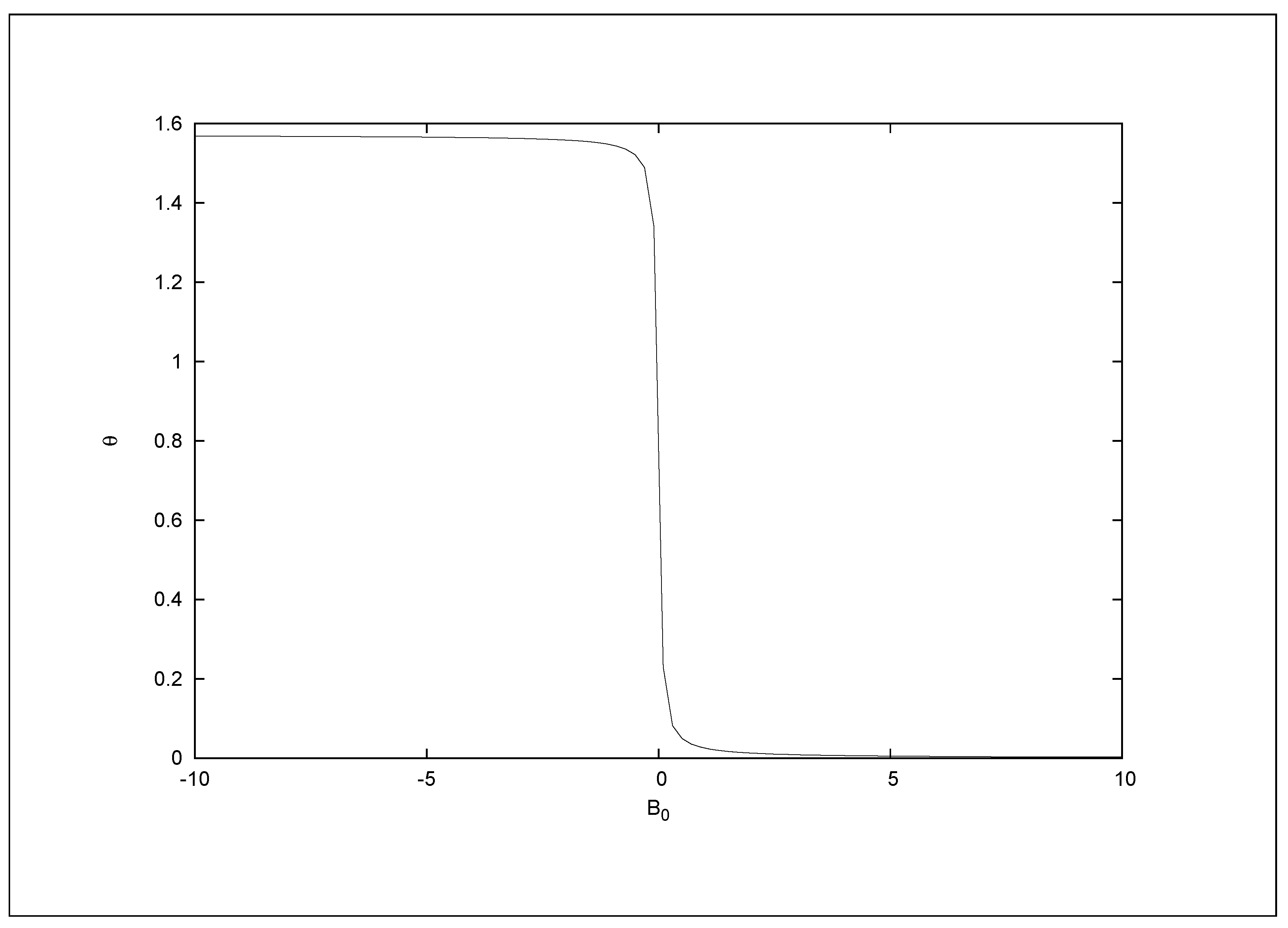
The phases independent of are associated with mixing angles and phases of neutrinos, e.g., (also ) and (also ). Therefore, depending on -s, which are determined by gravitational field and the physical nature of spacetime geometry, the -independent parts of phases vary. In the absence of gravitational field and in the presence of lepton number violating interaction and hence Majorana mass, neutrino and antineutrino mix with . Figure 3 shows that how the mixing angle of the basic neutrino-antineutrino states changes with gravitational coupling, which furthermore controls the geometric Berry-like phases associated with given in Section 4.1 and Section 4.2. While a stronger gravity effect kills oscillation, it still leads to a non-zero geometric phase.
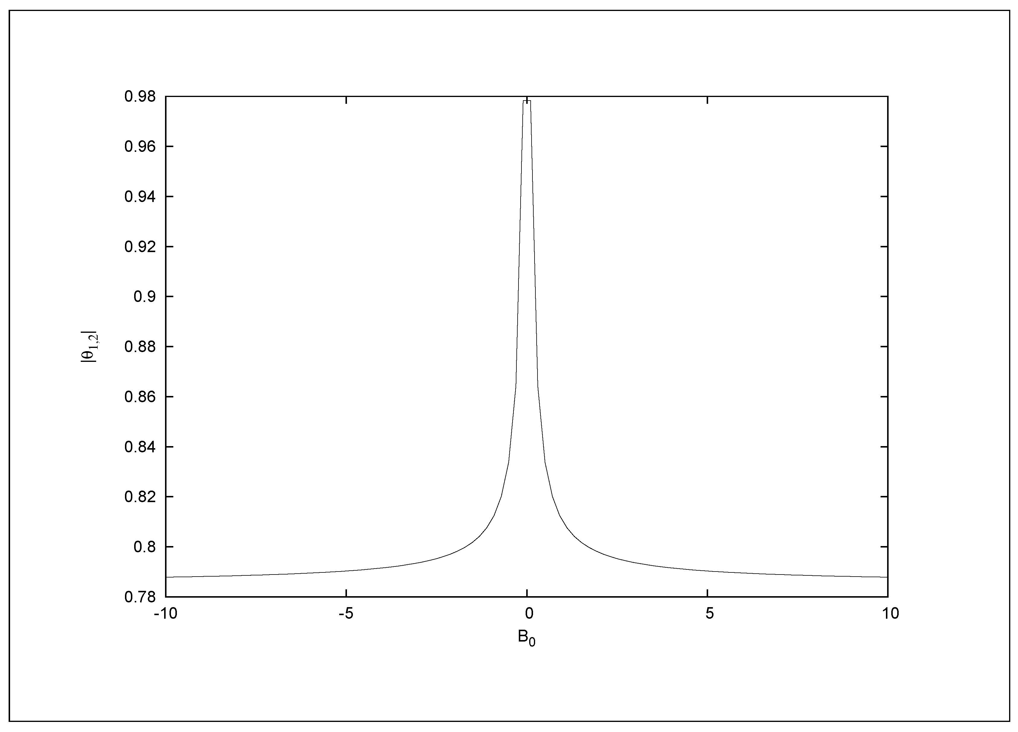
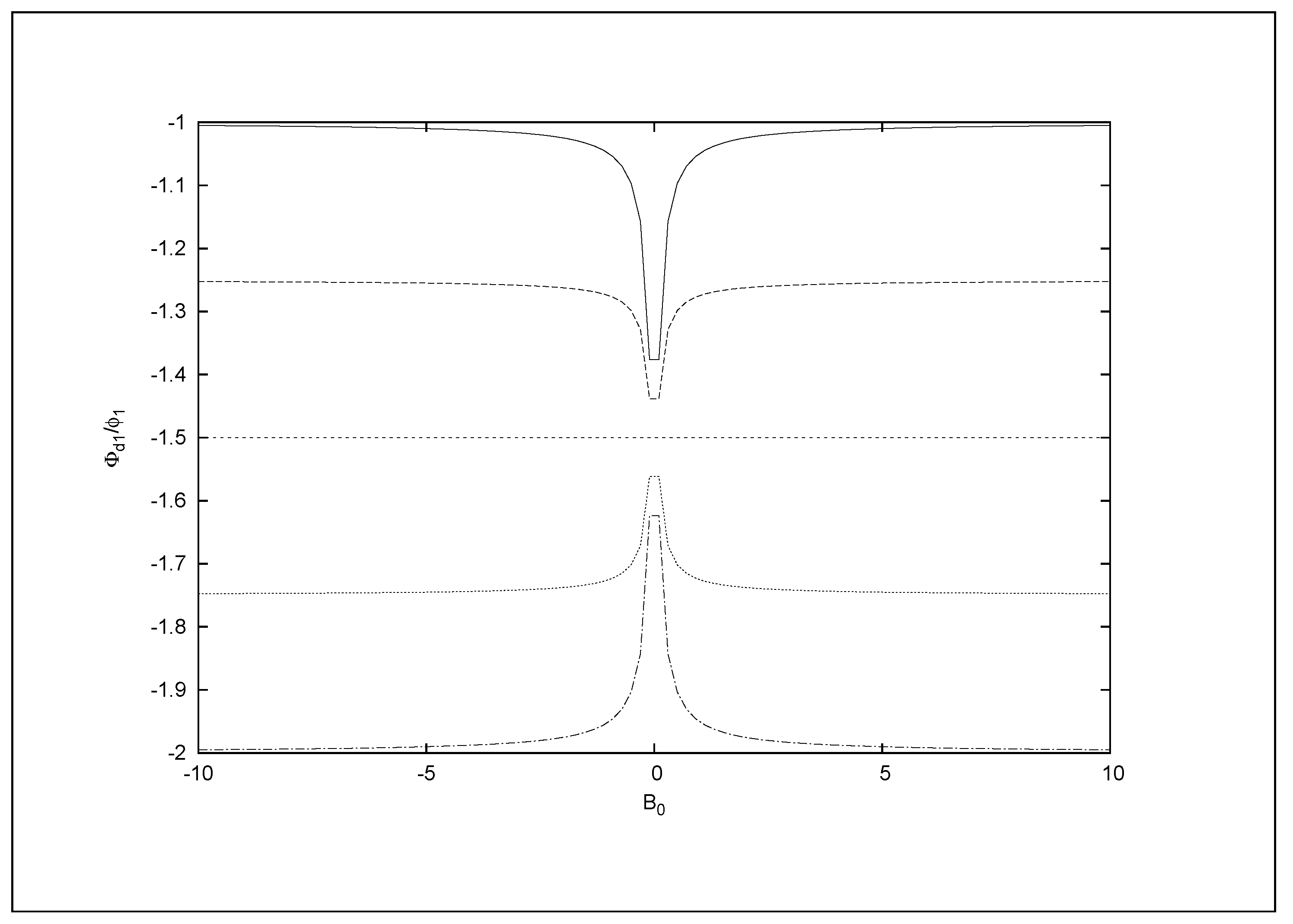
In the presence of very strong gravitational effect () (see, e.g., [25,26]), and for entangled states . Similarly, the -independent part of of entangled states survives even at a very strong gravitational field for an arbitrary . Figure 4 shows that and decrease with the increase of , which furthermore controls geometric Berry-like phases associated with entangled states given in Section 5. Figure 5 shows how the corresponding -independent part of varies with the change of the strength of gravitational coupling. This confirms that while decrease with increasing , mixing and also various phases still survive.
7. Summary
Spinors interacting with background gravity of arbitrary strength in an arbitrary spacetime are known to be split in energies between up and down spinors and furthermore into the states of positive and negative energies. The only requirement is that the spacetime should not be spherically symmetric. It has been shown that such spinors acquire a geometric phase due to background gravitational field in the same way as they do in a magnetic field. The necessary condition for such a situation is either the spacetime curvature coupling to the spinor (gravitational 4-vector potential) is not constant or the momentum of the spinor is not constant, along with a non-zero (even constant) temporal part of curvature coupling.
Neutrinos, as a class of spinors in nature, are shown to acquire geometric as well as dynamic phases during their propagation under background gravitational field. To have a non-trivial phase induced by the gravitational field of compact objects (e.g., black hole), the mass of the object producing gravitational fields must not be more than a millionth of a solar mass, i.e., primordial in nature. There are many missions to constrain the evidence for primordial black holes, e.g., observing specific small interference patterns within gamma-ray bursts by the Fermi Gamma-ray Space Telescope could be the indirect evidence for primordial black holes.
In the flavor sector, when the background gravity is much stronger than the lepton number violating (Majorana) masses, the mixing parameters become a constant equal to , hence maximum mixing, which could lead to -dependent geometric phases if varies. However, for a weak background gravity, are found to depend on the specific values of the neutrino masses. The combined neutrino–antineutrino states form an entangled system whose phases have also been calculated.
Author Contributions
Conceptualization, B.M. and S.K.G.; methodology, B.M. and S.K.G.; software, B.M.; validation, B.M.; formal analysis, B.M. and S.K.G.; investigation, B.M.; resources, B.M. and S.K.G.; data curation, B.M.; writing—original draft preparation, B.M.; writing—review and editing, B.M.; visualization, B.M.; supervision, B.M.; project administration, B.M.; funding acquisition, B.M. All authors have read and agreed to the published version of the manuscript.
Funding
This research received no external funding.
Acknowledgments
B.M. thanks Subhashish Banerjee of IIT Jodhpur, Kaushik Ghosh of Vivekananda College Kolkata, Tanuman Ghosh of RRI Bangalore, Subroto Mukerjee of IISc Bangalore for discussions at various stages of the work. Thanks are also due to Lars Andersson and Marius Oancea of AEI, Max-Planck Institute Potsdam-Golm, for discussions.
Conflicts of Interest
The authors declare no conflict of interest.
References
- Berry, M.V. Quantal phase factors accompanying adiabatic changes. Proc. R. Soc. A 1984, 392, 45. [Google Scholar]
- Aharonov, Y.; Anandan, J. Phase change during a cyclic quantum evolution. Phys. Rev. Lett. 1987, 58, 1593. [Google Scholar] [CrossRef] [PubMed]
- Samuel, J.; Bhandari, R. General setting for Berry’s phase. Phys. Rev. Lett. 1988, 60, 2339. [Google Scholar] [CrossRef] [PubMed]
- Mukunda, N.; Simon, R. Quantum kinematic approach to the geometric phase. I. General formalism. Ann. Phys. (N. Y.) 1993, 228, 205. [Google Scholar] [CrossRef]
- Nakagawa, N. Geometrical phase factors and higher-order adiabatic approximations. Ann. Phys. (N. Y.) 1987, 179, 145. [Google Scholar] [CrossRef]
- Vidal, J.; Wudka, J. Non-dynamical contributions to left-right transitions in the solar neutrino problem. Phys. Lett. B 1990, 249, 473. [Google Scholar] [CrossRef]
- Aneziris, C.; Schechter, J. Three Majorana neutrinos in a twisting magnetic field. Phys. Rev. D 1992, 45, 1053. [Google Scholar] [CrossRef]
- Smirnov, A.Y. The geometrical phase in neutrino spin precession and the solar neutrino problem. Phys. Lett. B 1991, 260, 161. [Google Scholar] [CrossRef]
- Guzzo, M.M.; Bellandi, J. On the question of neutrino spin precession in a magnetic field. Phys. Lett. B 1992, 294, 243. [Google Scholar] [CrossRef] [Green Version]
- He, X.-G.; Li, X.-Q.; McKellar, B.H.J.; Zhang, Y. Berry phase in neutrino oscillations. Phys. Rev. D 2005, 72, 053012. [Google Scholar] [CrossRef] [Green Version]
- Blasone, M.; Henning, P.A.; Vitiello, G. Berry phase for oscillating neutrinos. Phys. Lett. B 1999, 466, 262. [Google Scholar] [CrossRef] [Green Version]
- Wang, X.-B.; Kwek, L.C.; Liu, Y.; Oh, C.H. Noncyclic phase for neutrino oscillation. Phys. Rev. D 2001, 63, 053003. [Google Scholar] [CrossRef] [Green Version]
- Joshi, S.; Jain, S. Geometric phase for neutrino propagation in magnetic field. Phys. Lett. B 2016, 754, 135. [Google Scholar] [CrossRef] [Green Version]
- Ramaseshan, S.; Nityananda, R. The interference of polarized light as an early example of Berry’s phase. Curr. Sci. 1986, 55, 1225. [Google Scholar]
- Pancharatnam, S. Generalized theory of interference, and its applications. Proc. Indian Acad. Sci. A 1956, 44, 247. [Google Scholar] [CrossRef]
- Mehta, P. Topological phase in two flavor neutrino oscillations. Phys. Rev. D 2009, 79, 096013. [Google Scholar] [CrossRef] [Green Version]
- Dajka, J.; Syska, J.; Łuczka, J. Geometric phase of neutrino propagating through dissipative matter. Phys. Rev. D 2011, 83, 097302. [Google Scholar] [CrossRef] [Green Version]
- Syska, J.; Dajka, J.; Łuczka, J. Interference phenomenon and geometric phase for Dirac neutrino in π+ decay. Phys. Rev. D 2013, 87, 117302. [Google Scholar] [CrossRef] [Green Version]
- Joshi, S.; Jain, S.R. Noncyclic geometric phases and helicity transitions for neutrino oscillations in a magnetic field. Phys. Rev. D 2017, 96, 096004. [Google Scholar] [CrossRef] [Green Version]
- Johns, L.; Fuller, G.M. Geometric phases in neutrino oscillations with nonlinear refraction. Phys. Rev. D 2017, 95, 043003. [Google Scholar] [CrossRef] [Green Version]
- Wang, Z.; Pan, H. Exploration of CPT violation via time-dependent geometric quantities embedded in neutrino oscillation through fluctuating matter. Nuc. Phys. B 2017, 915, 414. [Google Scholar] [CrossRef] [Green Version]
- Dixit, K.; Alok, A.K.; Banerjee, S.; Kumar, D. Geometric phase and neutrino mass hierarchy problem. J. Phys. G 2018, 45, 085002. [Google Scholar] [CrossRef] [Green Version]
- Capolupo, A.; Giampaolo, S.M.; Hiesmayr, B.C.; Vitiello, G. Geometric phase of neutrinos: Differences between Dirac and Majorana neutrinos. Phys. Lett. B 2018, 780, 216. [Google Scholar] [CrossRef]
- Simonov, K.; Capolupo, A.; Giampaolo, S.M. Gravity, entanglement and CPT-symmetry violation in particle mixing. Eur. Phys. J. C 2019, 79, 902. [Google Scholar] [CrossRef] [Green Version]
- Mukhopadhyay, B. Gravity-induced neutrino-antineutrino oscillation: CPT and lepton number non-conservation under gravity. Class. Quantum Gravity 2007, 24, 1433. [Google Scholar] [CrossRef] [Green Version]
- Sinha, M.; Mukhopadhyay, B. CPT and lepton number violation in the neutrino sector: Modified mass matrix and oscillation due to gravity. Phys. Rev. D 2008, 77, 025003. [Google Scholar] [CrossRef] [Green Version]
- Singh, P.; Mukhopadhyay, B. Gravitationally induced neutrino asymmetry. Mod. Phys. Lett. A 2003, 18, 779. [Google Scholar] [CrossRef] [Green Version]
- Mukhopadhyay, B. Neutrino asymmetry around black holes: Neutrinos interact with gravity. Mod. Phys. Lett. A 2005, 20, 2145. [Google Scholar] [CrossRef] [Green Version]
- Debnath, U.; Mukhopadhyay, B.; Dadhich, N. Spacetime Curvature Coupling of Spinors in Early Universe:. Neutrino Asymmetry and a Possible Source of Baryogenesis. Mod. Phys. Lett. A 2006, 21, 399. [Google Scholar] [CrossRef] [Green Version]
- Kim, C.W.; Sze, W.K.; Nussinov, S. Neutrino oscillations and the Landau-Zener formula. Phys. Rev. D 1987, 35, 4014. [Google Scholar] [CrossRef]
- Stodolsky, L. Treatment of neutrino oscillations in a thermal environment. Phys. Rev. D 1987, 36, 2273. [Google Scholar] [CrossRef] [PubMed]
- Píriz, D.; Roy, M.; Wudka, J. Neutrino oscillations in strong gravitational fields. Phys. Rev. D 1996, 54, 1587. [Google Scholar] [CrossRef] [PubMed] [Green Version]
- Mohanty, S.; Mukhopadhyay, B.; Prasanna, A.R. Experimental tests of curvature couplings of fermions in general relativity. Phys. Rev. D 2002, 65, 122001. [Google Scholar] [CrossRef] [Green Version]
- Dixit, K.; Naikoo, J.; Mukhopadhyay, B.; Banerjee, S. Quantum correlations in neutrino oscillations in curved spacetime. Phys. Rev. D 2019, 100, 055021. [Google Scholar] [CrossRef] [Green Version]
- Birrell, N.D.; Davies, P. Quantum Fields in Curved Space; Cambridge University Press: Cambridge, UK, 1982. [Google Scholar]
- Kaku, M. Quantum Field Theory; Oxford University Press: Oxford, UK, 1993. [Google Scholar]
- Schwinger, J. Particles, Sources, and Fields III; Addison-Wesley: Redwood City, CA, USA, 1989. [Google Scholar]
- Obukhov, Y.N. Spin, Gravity, and Inertia. Phys. Rev. Lett. 2001, 86, 192. [Google Scholar] [CrossRef] [Green Version]
- Huang, X.; Parker, L. Hermiticity of the Dirac Hamiltonian in curved spacetime. Phys. Rev. D 2009, 79, 024020. [Google Scholar] [CrossRef] [Green Version]
- Mukhopadhyay, B. Exploring the Universe: From Near Space to Extra-Galactic. In Astrophysics and Space Science Proceedings; Mukhopadhyay, B., Sasmal, S., Eds.; Springer: Berlin/Heidelberg, Germany, 2018; Volume 53, p. 3. [Google Scholar]
- Colladay, D.; Kostelecký, V.A. CPT violation and the standard model. Phys. Rev. D 1997, 55, 6760. [Google Scholar] [CrossRef] [Green Version]
- Ellis, J.; Mavromatos, N.E. Role of space-time foam in breaking supersymmetry via the Barbero-Immirzi parameter. Phys. Rev. D 2011, 84, 085016. [Google Scholar] [CrossRef] [Green Version]
- Mavromatos, N.E.; Sarkar, S. CPT-violating leptogenesis induced by gravitational defects. Eur. Phys. J. C 2013, 73, 2359. [Google Scholar] [CrossRef] [Green Version]
- Mosquera Cuesta, H.J. Neutrino astrophysics in slowly rotating spacetimes permeated by nonlinear electrodynamics fields. Astrophys. J. 2017, 835, 215. [Google Scholar] [CrossRef]
- Diaz, J.S.; Katori, T.; Spitz, J.; Conrad, J.M. Search for neutrino-antineutrino oscillations with a reactor experiment. Phys. Lett. B 2013, 727, 412. [Google Scholar] [CrossRef] [Green Version]
- Shapiro, S.L.; Teukolsky, S.A. Black Holes, White Dwarfs, and Neutron Stars: The Physics of Compact Objects; John Wiley & Sons: New York, NY, USA, 1983. [Google Scholar]
- Sjöqvist, E. Geometric phase for entangled spin pairs. Phys. Rev. A 2000, 62, 022109. [Google Scholar] [CrossRef]
| 1. | Note that the corresponding temperature GeV [46]. |
Figure 1.
Zeeman-splitting in the electromagnetic case.

Figure 2.
Gravitational “Zeeman-splitting”.

Figure 3.
Variation of mixing angle in radian of basic neutrino–antineutrino mixing as a function of gravitational coupling in units of eV with eV.
Figure 3.
Variation of mixing angle in radian of basic neutrino–antineutrino mixing as a function of gravitational coupling in units of eV with eV.

Figure 4.
Variation of flavor mixing angles in radian as functions of gravitational coupling in units of eV with eV, eV and eV.
Figure 4.
Variation of flavor mixing angles in radian as functions of gravitational coupling in units of eV with eV, eV and eV.

Figure 5.
Variation of -independent part of for entangled states as a function of gravitational coupling in units of eV with eV, eV and eV, and . From top to bottom, lines are for and .
Figure 5.
Variation of -independent part of for entangled states as a function of gravitational coupling in units of eV with eV, eV and eV, and . From top to bottom, lines are for and .

© 2020 by the authors. Licensee MDPI, Basel, Switzerland. This article is an open access article distributed under the terms and conditions of the Creative Commons Attribution (CC BY) license (http://creativecommons.org/licenses/by/4.0/).
Share and Cite
MDPI and ACS Style
Mukhopadhyay, B.; Ganguly, S.K. Gravity-Induced Geometric Phases and Entanglement in Spinors and Neutrinos: Gravitational Zeeman Effect. Universe 2020, 6, 160. https://doi.org/10.3390/universe6100160
AMA Style
Mukhopadhyay B, Ganguly SK. Gravity-Induced Geometric Phases and Entanglement in Spinors and Neutrinos: Gravitational Zeeman Effect. Universe. 2020; 6(10):160. https://doi.org/10.3390/universe6100160
Chicago/Turabian StyleMukhopadhyay, Banibrata, and Soumya Kanti Ganguly. 2020. "Gravity-Induced Geometric Phases and Entanglement in Spinors and Neutrinos: Gravitational Zeeman Effect" Universe 6, no. 10: 160. https://doi.org/10.3390/universe6100160
Note that from the first issue of 2016, this journal uses article numbers instead of page numbers. See further details here.