Enhancing Information Content in the Satellite-Derived Daytime Infrared Sea Surface Temperature Dataset Using a Transformative Approach

Introduction

Sea Surface Temperature (SST) is one of the crucial variables in the earth science modeling (e.g., numerical weather prediction, ocean circulation modeling, air−sea interactions, marine ecosystems, upwelling regions, boundary currents, planetary boundary layer divergence, ocean biology, including coral reefs and algae blooms) (for example, Fèvre, 1987; Largier, 1993; Turiel et al., 2008; Castillo and Lima, 2010; Knievel et al., 2010; Sirjacobs et al., 2011; Dufois and Rouault, 2012; Gawarkiewicz et al., 2012; Callies et al., 2015; Huang and Feng, 2015; Chatterjee et al., 2019). SST gradient fields are often used to derive the water masses of marine thermal fronts, thereby regional optimal conditions for the growth of marine phytoplankton are identified with respect to upwellings, nutrients’ exchanges (CO₂), and mixing of oceanic layers (Behrenfeld and Falkowski, 1997; Acha et al., 2004; Saraceno et al., 2005; Behrenfeld et al., 2006; Rivas and Pisoni, 2010; Williams et al., 2013). The temporal and spatial anomalies in SST fields are used to study the ecosystems of fisheries (Santos, 2000; Zainuddin et al., 2006). Apart from many physical and biological oceanographic applications, SST is also used for generating services (e.g., potential fishing zone advisories). As more than 70% of the earth’s surface is covered by oceans, an accurate determination of the global SSTs with high temporal and spatial resolutions will help to understand composite earth system studies.

Sea Surface Temperature is also a critical component for the study of the interface of the ocean and the atmosphere, e.g., the exchanges of heat (sensible heat flux, latent heat flux, and long-wave radiation), moisture, momentum, and gasses between the two (for example, Wanninkhof et al., 2009; Dufois and Rouault, 2012; Bentamy et al., 2017). SST eddies and fronts are used to explain sub-surface dynamics in terms of surface thermal expansion (for example, Tandeo et al., 2014 January). The atmospheric boundary layer is studied using the variation in the exchanges of surface momentum across the thermal gradients (e.g., Mcphaden et al., 2006; Minobe et al., 2008; O’Neill et al., 2010; Perlin et al., 2014). Variations in the SST values impact several components of the climate and global circulation models (e.g., Jha et al., 2013; Dong et al., 2018). Satellite-derived SSTs are used for some scientific applications where the society is directly benefitted, viz. severe storms’ prediction, sea-level rise, numerical weather prediction, and estimation of ocean heat content. Thus, the precise determination of SST values is of immense importance to explore and discover the ocean as well as to better understand the earth sciences. In the wake of this need, Physical Deterministic SST retrieval (PDSST) suite for nighttime scenarios has already been developed using a transformative approach of the physical deterministic inverse method, where the parameter values are quantified by inverting the Radiative Transfer (RT) model (e.g., Koner et al., 2015, 2016b; Koner and Harris, 2016a,b; Koner, 2018, 2020b). However, as per the literature survey, most operational regression-based SST retrieval schemes do not use the measurements from Mid Wave Infrared (MWIR) channels for daytime SST retrieval due to solar contamination. On the other hand, the incorporation of MWIR channels in the PDSST scheme is straight forward. As the incorporation of MWIR channels in daytime SST retrieval is a first of its kind, a thorough investigation is presented here.

Physical Deterministic Sea Surface Temperature scheme has already been applied to the MODIS-AQUA radiance data for retrieving the SST and is reported in earlier publications (Koner and Harris, 2016a,b), where the validation has been made using millions of global matchups and nighttime scenarios. The PDSST suite has also applied to daytime SST retrieval from MODIS-AQUA using global matchups in Koner, 2020b. This study mainly focusses on the detailed performances of PDSST for coastal areas using swath processed data. The enhanced information content of daytime SSTs in PDSST retrieval is discussed in terms of both the quality and Data Coverage (DC) of the swath-processed daytime SSTs from MODIS-AQUA. The MODIS instrument is considered here for the case study to evaluate the performances of the daytime SST retrievals using MWIR channels in the PDSST suite because MODIS has been providing unique high-quality radiance data for almost two decades and geophysical parameter values from these measurements are greatly important for many geoscience models. Also, only the MODIS instrument has three MWIR channels which can help to understand the importance of MWIR in daytime SST retrieval. The quality of SSTs is measured by Root Mean Squared Differences (RMSD) from the values of in situ matches. The DC is defined by the number of cloud-free pixels for swath-processed SSTs as compared to the total number of ocean pixels in a granule. A detailed comparison between the daytime SST retrieval using the Physical Deterministic Sea Surface Temperature suite, including MWIR channels, and operational Regression-based daytime MODIS SSTs (RGSSTs), obtained from Physical Oceanography Distributed Active Archive Center (PO.DAAC), is conducted to address the information gain by PDSST scheme. Elaborately, Section “Description of PDSST Suite” provides a short description of the PDSST-suite. Section “Verification of Fast Forward Model” demonstrates the usability of the publicly available Community Radiative Transfer Model (CRTM v2.3), NOAA for daytime SST retrieval. Section “Comparison and Validation of PDSSTs” addresses the comparison and quantitative validation of swath processed SSTs using PDSST and RGSST from MODIS-AQUA, for coastal and near-coastal regions, using in situ matches obtained from NOAA website (Xu and Ignatov, 2014). Section “Cloud Detection and Quality Flag” discusses the cloud detection issue, using the Cloud and Error Masking (CEM) in PDSST-suite, and Quality Flag (QF) obtained from PO.DAAC database. Section “PDSST for Oceanic Fronts’ Study” focuses on the quality of the swath-processed daytime SSTs using the PDSST scheme in relevance to oceanic fronts’ study. Section “Results and Discussions” includes the results and discussions.

Description of PDSST Suite

Physical Deterministic Sea Surface Temperature suite is, based on a transformative approach, comprised of a physical deterministic retrieval algorithm (truncated total least squares), and a quasi-deterministic cloud detection algorithm, namely CEM (Koner et al., 2016b). Unlike any stochastic approach, the PDSST suite is applied on a single pixel without the error being treated as information. As per literature (Koner et al., 2015; Koner and Harris, 2016b; Koner, 2020b), PDSST retrieval algorithm for daytime multichannel MODIS-AQUA is as follows:

Where, x_ttls is the retrieved state vector, I is the identity matrix, K is the Jacobian, x_ig is the initial guess of the state vector, Δy_δ is the residual (i.e., observation – model) and λ is regularization constraint parameter. The three parameters in the state vector (x_ttls) are [slog⁡(w)log⁡(a)], where w is Total Column Water Vapor (TCWV), s is SST, and a is the sum of total columns of all aerosols. The unprecedented capability of the PDSST algorithm is that aerosol is used in a forward model calculation as well as in the retrieved vector. Global Forecast Simulation (GFS) data are used as input for CRTM. Two out of six channels (3.9, 4, 4.5, 11, 13.4, and 13.6 μm) in the PDSST algorithm are considered from the MWIR band. On the other hand, both operational products of RGSST from MODIS and Microwave SST (MWSST) from Advanced Microwave Scanning Radiometer (AMSR2), obtained from the Remote Sensing Systems (RSS) website, are based on the regression method. RGSST from the MODIS retrieval algorithm uses only the two channels of 11 and 12 μm for daytime.

The CEM algorithm is mainly based on functional spectral differences and double differences between model and measurements (Koner and Harris, 2016a; Koner et al., 2016b; Koner, 2018) as follows:

Where, ${\text{T}}_{\text{ch}}^{\text{t}}$ stands for the Brightness Temperature (BT) of the channel “ch” and the type “t” (either measurement “m” or calculated using RT model “c”). θ_spec is the specular angle. $dd(3.9,4)={\text{T}}_{3.9}^{\text{m}}-{\text{T}}_4^{\text{m}}-{\text{T}}_{3.9}^{\text{c}}+{\text{T}}_4^{\text{c}}$ is the double differences between 3.9 and 4 μm channels. Similarly, $dd(3.9,11)={\text{T}}_{3.9}^{\text{m}}-{\text{T}}_{11}^{\text{m}}-{\text{T}}_{3.9}^{\text{c}}+{\text{T}}_{11}^{\text{c}}$ is the double differences between 3.9 and 11 μm channels. $rt{v}_{3.9}=({\text{T}}_{3.9}^{\text{m}}-{\text{T}}_{3.9}^{\text{c}})/{\text{K}}_{3.9}^{\text{sst}}$ is the single channel retrieval update of 3.9 μm channel and ${\text{K}}_{3.9}^{\text{sst}}$ is the Jacobian of 3.9 μm channel with respect to SST. Similarly, rtv₁₁ is the single channel retrieval update of 11 μm channel.

Since cloud detection cannot be implemented using a deterministic inverse method due to the severe lack of the measurements as compared to the number of unknowns in the cloud detection problem, an additional RT-based test is held to get a more robust performance from CEM such that the pixels are discarded if rtv_3.9 is less than −2 K and abs(rtv_3.9−rtv₁₁) is greater than 0.5 K. Although the spatial test is not based on sound physics, it helps to improve the detection capability and so, most operational cloud detection algorithms use the spatial test. The spatial test for CEM is highly flexible. The targeted pixel is discarded if the difference in the value of maximum and minimum of the surrounding 3 × 3 pixels of the measured 3.9 μm channel is more than 2.5 K. Also, the difference of the measured BT value of the targeted 11 μm channel and the maximum value in the neighborhood of 3 × 3 pixels should be less than 0.75 K for being cloud-free.

As there is an absence of the cloud flag field in the RGSST from PO.DAAC database, the highest value of QF = 5 (RGSST5) is considered as the cloud-free subset. The values of QF are determined by some threshold-based criteria.

Verification of Fast Forward Model

The calculated BTs of MWIR channels using CRTM v2.3 for swath-processed SST retrieval are tested in this section. For demonstration, a single granule of MODIS-AQUA is carefully chosen using the following considerations: (a) a large number of in situ measurements for ground verification, (b) a wide variation in the values of θ_spec, including θ_spec < 10°, to understand the effect of “Glint” reflection for PDSST retrieval, and (c) less cloudy area. A granule from the Chesapeake Bay (CB) on July 13, 2019, is considered for this study. There are 68 in situ measurements and the values of θ_spec for a significant number of pixels are less than 10° as are shown in Figure 1A. The “nighttime equivalent” simulated BTs of 3.9 μm channel are calculated using CRTM v2.3 where all input parameters for CRTM are kept the same except only adding 90° to the solar zenith angle. The calculated BT differences of 3.9 μm channel between daytime and “nighttime equivalent” using CRTM v2.3 are shown in Figure 1B. The difference values of BTs are noticeable when θ_spec < 30° and 10 K difference is observed when θ_spec < 10°, as shown in Figure 1B. The calculated BT differences of 3.9 μm channel using CRTM v2.3 for MWIR seem to be reasonable for daytime scenarios as similar to the global matchup study (Koner, 2020b).

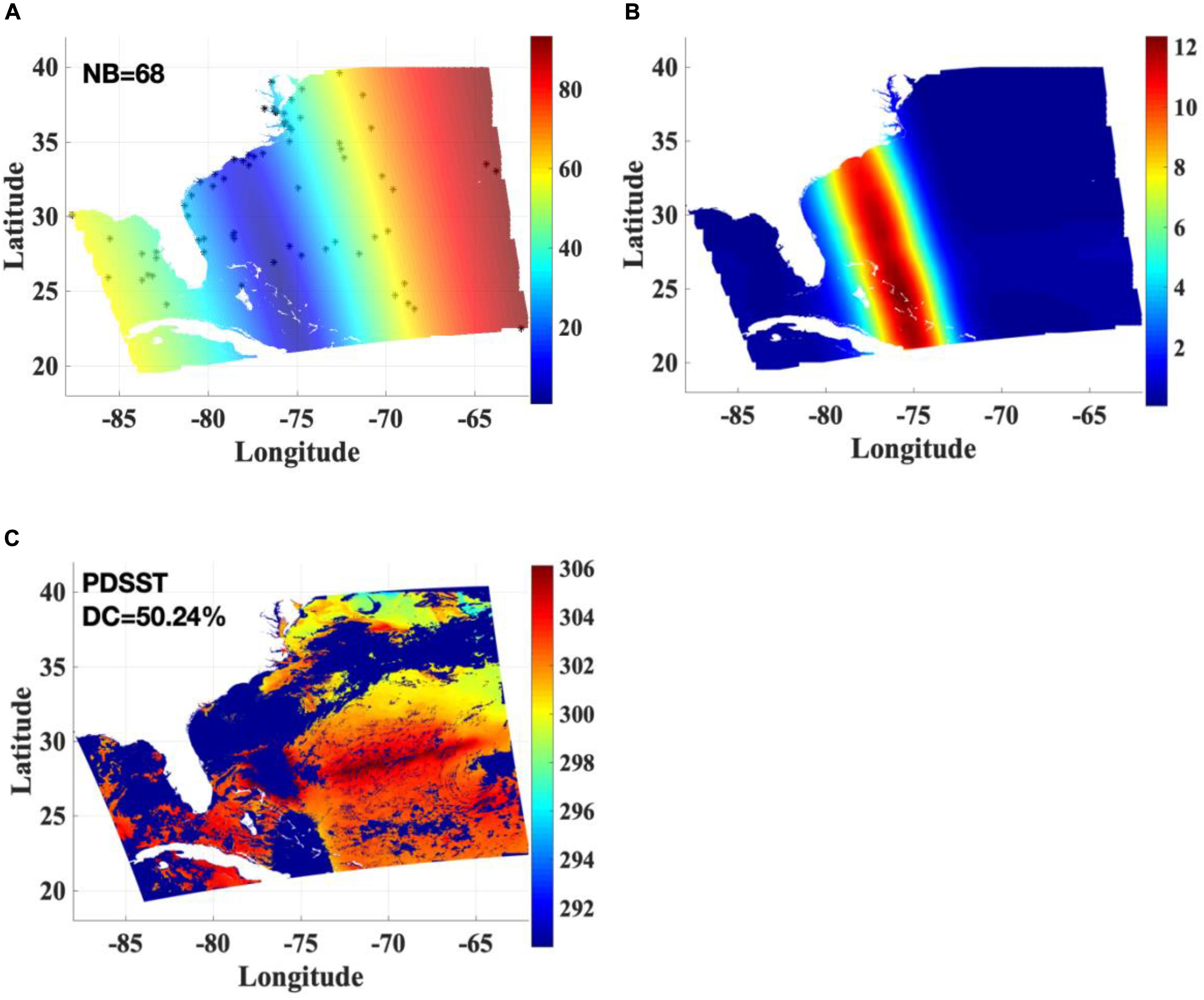
Figure 1. Single swath maps: (A) Specular angle (θ_spec) and the locations of in situ (Unit of color bar is degree), (B) Differences of the simulated BTs of 3.9 μm channel between daytime and “nighttime equivalent” using CRTM (Unit of color bar is K), and (C) Retrieved SSTs using PDSST-suite (Unit of color bar is K). In situ locations are plotted using “*”. DC and NB stand for data coverage (cloud-free pixels) and the numbers of buoys, respectively. The ranges of longitude and latitude from −180° to 180° and from −90° to 90° represent West to East and South to North, respectively.

The retrieved SSTs using PDSST-suite are shown in Figure 1C. PDSST-suite finds that 50.24% of the total pixels over the water body and 11 out of 68 in situ locations are cloud-free. The number of cloud-free in situ according to PDSST-suite is 6 for the region when θ_spec < 30° by applying the constraint −79° < Longitude < −73°. The values of RMSD are 0.32 K using 11 in situ and 0.28 K using 6 in situ for full-swath and θ_spec < 30°, respectively. The validation results against in situ produce strong assurance that the simulated BTs of MWIR channels using CRTM v2.3 can be safely used for daytime SST retrieval. However, it is observed that PDSST-suite finds that a significant portion of this granule is masked as cloudy when θ_spec < 10° (around the longitude −75°). The reason for it is beyond the scope of this paper and an elaborate investigation will be conducted in the future. Note that the longitude and latitude scales are −180° to 180° and −90° to 90° due to the simplicity of the plot. This implies that the positive values of longitude and latitude represent the East and North, respectively and the negative values of longitude and latitude represent the West and South, respectively.

To illustrate the advantage of using MWIR channels in the PDSST-suite with respect to the quality of retrieved daytime SSTs, PDSST retrievals are compared with the conventional regression-based daytime SSTs, where MWIR channels are not used, obtained from PO.DAAC, as shown in Figure 2. The retrieved SST map of RGSST5, for QF = 5, are shown in Figure 2A using the same granule as shown in Figure 1C. The value of RMSD using 4 matched in situ is 0.44 K, which is ∼40% more compared to the same for PDSST (0.32 K). The DC for RGSST5 is 21.05%, which is less than half of the DC from PDSST (50.24%). It is observed from Figure 2A that most of the regions where θ_spec < 30° are masked by a low value of QF in the PO.DAAC database and are shown as empty (deep blue color in Figure 2A). The quality of PDSST for the region of θ_spec < 30° cannot be verified by comparing it with the values of RGSST5, thus, the flagging threshold is decreased up to QF ≥ 3 (RGSST3), and is plotted in Figure 2B. The DC for RGSST3 increases drastically to 44.12% as compared to the same for RGSST5, but still is lower than PDSST (50.24%). The RMSD value of RGSST3 is 1.21 K using 10 matched in situ, which is more than double compared to the same from the RGSST5. Although, the DC for RGSST3 is higher than the same for PDSST for the region of θ_spec < 30°, the RMSD value is 1.44 K using 6 in situ matches for this region, which is significantly high. By qualitatively comparing the SST maps of PDSST and RGSST3, it can be concluded that MWIR channels in PDSST-suite can be safely used to improve the quality of SSTs.

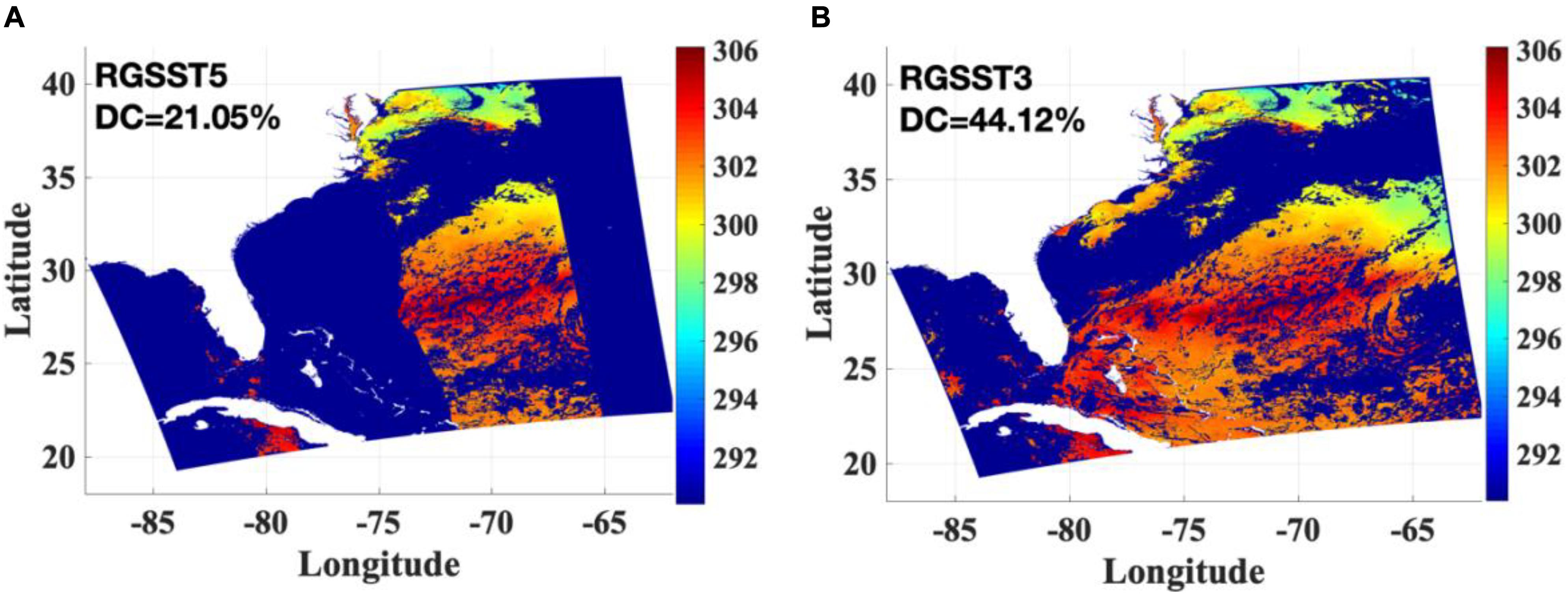
Figure 2. Regression-based SST maps for the same granule of Figure 1, obtained from PO.DAAC website: (A) RGSST5 at QF = 5 and (B) RGSST3 at QF ≥ 3. DC stands for data coverage. The ranges of longitude and latitude from −180° to 180° and from −90° to 90° represent West to East and South to North, respectively. Unit of color bar is K.

Comparison and Validation of PDSSTs

It has been found from the global map of monthly matchups study (Koner and Harris, 2016b; Koner, 2020b) that the number of in situ matches by PDSST is higher with a comparative lower error than RGSSTs from MODIS-AQUA for the dynamic oceanographic regions and the coastal areas of oceans. It can be explained that the coefficients for regression-based SST retrieval are conventionally generated using global matches and drifter buoys only, which may not be suitable for SST retrievals from the coastal regions due to highly dynamic atmospheric conditions and a lack of sufficient drifters for the said region. On the other hand, the PDSST algorithm never directly uses in situ for satellite-derived SST retrievals and produces homogenous retrieval results without any influence of in situ.

Although several dynamic oceanographic regions are studied, the California Coast (CC) in the Pacific Ocean, the CB in the Atlantic Ocean, and the Bay of Bengal (BB) in the Indian Ocean (IO) are focused on in this study for an illustration. CC is a highly dynamic location with a strong exchange of materials and energies between the aquatic, atmosphere, and terrestrial environments as well as intense chemical, biological, and physical interactions (for example, Lorenzo and Mantua, 2016) and SST is one important parameter for understanding these interactions. The economically valuable CB ecosystem is important for fisheries, recreation, navigation, and tourism (for example, Preston, 2004) and the key factors for the study of the vulnerability of aquatic, estuarine, and marine organisms is SST. A large number of buoys are deployed for both regions of CC and CB, which can be used for quantitative validation purposes. On the other hand, BB is a highly variable and dynamically complex system under the monsoonal influence and contains numerous downwelling eddies, Indian Ocean Dipole, boundary currents, but the in situ measurements are very sparse. This leads to satellite-derived SSTs being highly important to develop a reasonable ocean model for IO.

All relevant granules for the CC area are obtained using a constraint of −140° < longitude < −100° and 10° < latitude < 55° on the geo-locational data. Although the comparative study using both PDSST and RGSST5 is conducted for several months, the results of December 2017 and October 2019 are presented here for demonstration. There are 20 granules with 590 buoy matches and 21 granules with 670 buoy matches for October 2019 and December 2017, respectively. The detailed statistics of these granules in terms of the percentage of ocean cover (OC), the number of total matched buoys (NB), percentage of cloud-free pixels with respect to the total number of ocean pixels as per PDSST [DC (pd)] and RGSST5 [DC (rg)], number of buoys in the cloud-free set for PDSST [NB (pd)] and RGSST5 [NB (rg)] and RMSD of PDSST [ε (pd)] and RGSST5 [ε (rg)] are shown in Tables 1, 2.

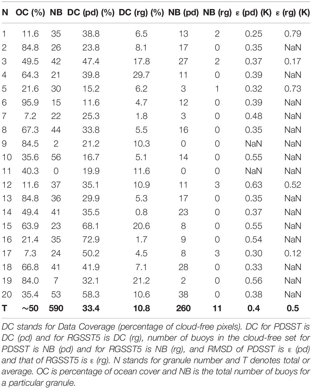
Table 1. Statistical information of retrieved results for 20 granules from CC using two different methods of PDSST and RGSST5 for the month of October 2019.

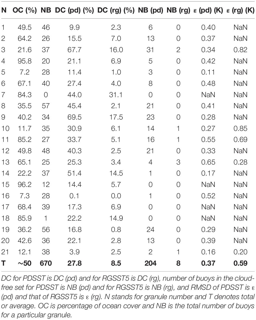
Table 2. Statistical information of retrieved results for 21 granules from CC using two different methods of PDSST and RGSST5 for the month of December 2017.

The average DC of PDSST is 33.4%, whereas the DC of RGSST5 is only 10.8% in terms of ocean-only pixels from Table 1 and similarly, DC of PDSST and RGSST5 are 27.8% and 8.5%, respectively, from Table 2. This implies ∼3 times more valuable SST data, for the dynamic areas of oceans, can be obtained using PDSST over RGSST5. Although the quality of retrieved SSTs for all pixels of these granules cannot be verified, a first order validation has been made using the matched buoy measurements. The total number of matched buoy measurements for the abovementioned region for the month of December 2017 is 670 (see Table 2). PDSST suite identifies 204 buoy measurements that can be used for the validation as cloud-free, whereas RGSST5 detects only 8 cloud-free buoy measurements. This implies that PDSST yields ∼25 times more DC over RGSST5 according to the match-up study for the dynamic area of CC. The average RMSD value of PDSST using 204 buoy measurements is ∼0.37 K. The average RMSD value of RGSST5 is 0.59 K, however, the validation using only 8 measurements is questionable. Improvement in information content for satellite-derived SSTs, using a transformative approach, refers to a dual benefit of increased DC and reduced error. Additionally, PDSST uses more channels than RGSST to exploit greater information from measurement and added local atmospheric information through GFS data. The overall information gains (G_inf) of PDSST by combining the increased DC and reduced RMSD using matchup data is introduced (Koner, 2020b) as:

It is found that the values of Ginf in terms of swath DC and RMSD from match-up buoys are ∼390% and ∼520% for the months of October 2019 and December 2017, respectively.

Similarly, CB region is outlined using a constraint of −100° < longitude < −60° and −10° < latitude < 55° on the geolocational data. For the demonstration, the statistics of 19 granules for the month of September 2019 are shown in Table 3. The number of matched buoys at QF = 5 for RGSST5 is 194, which is higher than the same for CC. PDSST finds that 360 buoys, out of 1095, are cloud-free. The RMSD values are 0.36 K and 0.47 K and DC values are 38.3% and 16% for PDSST and RGSST5, respectively. The information gain of PDSST over RGSST5 is ∼310%.

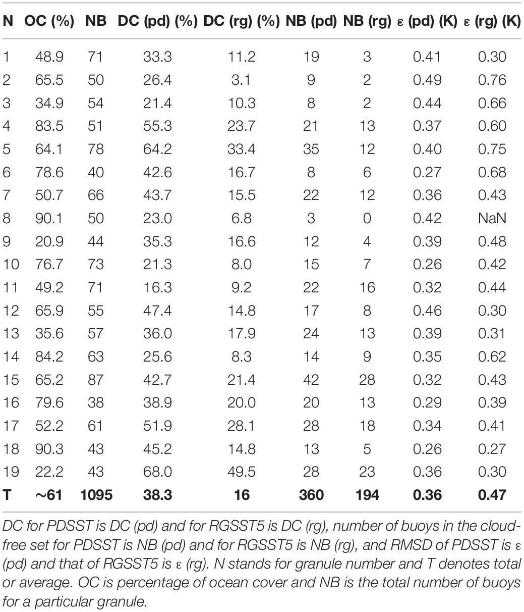
Table 3. Statistical information of retrieved results for 19 granules from CB using two different methods of PDSST and RGSST5 for the month of September 2019.

Bay of Bengal region is also outlined using a constraint of 67° < longitude < 100° and −10° < latitude < 30° on the geolocational data. The statistics of 18 granules for the month of December 2017 are shown in Table 4. The number of matched buoys at QF = 5 for RGSST5 is only 3 while PDSST sees only 6 buoy matches. It is very difficult to get a reasonable amount of buoy matches surrounding the coastal area of BB to conduct reasonable quantitative validations. Thus, a study on a region at Madagascar Coast (MC) in the IO is made to achieve some confidence on the quantitative validation of PDSST over the IO, including more areas from the deeper parts of the ocean to get more buoy matches, using a constraint of 30° < longitude < 80° and −40° < latitude < 0° on the geolocational data for the month of August 2019.

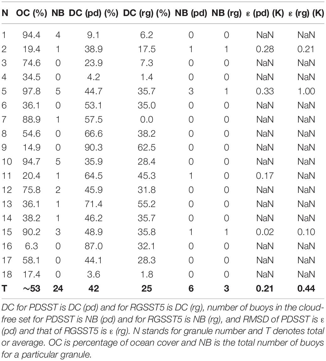
Table 4. Statistical information of retrieved results for 18 granules from BB using two different methods of PDSST and RGSST5 for the month of December 2017.

The detailed statistics of 38 granules are shown in Table 5. The RMSD value of PDSSTs using 48 buoy measurements is ∼0.27 K, and the RMSD value of RGSST5 SSTs is 0.41 K using 17 buoy measurements. The values of DC are 48.7% and 22.9% for PDSST and RGSST5, respectively. The information gain of PDSST over RGSST55 is ∼320%, which is comparable with CB and lower than CC.

Table 5. Statistical information of retrieved results for 38 granules from MC using two different methods of PDSST and RGSST5 for the month of August 2019.

Although the above validations of PDSST against in situ are highly satisfactory, a simplified Triple Collocation Method (TCM) is applied (cf. Stoffelen, 1998) on the point matchups to assess the regional true noise associated with PDSST retrievals in the context of skin temperatures. It is assumed in TCM that any dataset consists of a hypothetical truth corrupted by a noise: R_i = T + n_i, where R is retrieved data, T is hypothetical truth, i represents a dataset (1, 2, 3) and n is noise. Noise (n) has two components: the systematic part, which is referred to as bias (b), and the random part (σ).

Using three collocated datasets representing the same physical quantity (“alike”), individual σ_i values can be separated out if they are uncorrelated:

Using Eqn. 8 and further expanding:

If the random errors of the three “alike” datasets (σ₁,σ₂,σ₃) are uncorrelated, then: σ₁σ₂ = σ₁σ₃ = σ₂σ₃ = 0. Following this, one can find the true random error in data set R₁. Here, R₁, R₂ and R₃ correspond to the SSTs from PDSST and RGSST5, and the collocated buoy measurements, respectively. To explain further in the context of SSTs, one may raise the question that the errors are correlated if any two of the above-mentioned retrievals are from the same sensor. It is expected that correlated error would be negligibly small due to the fact that the applied inverse methods are in different paradigms and the errors in measured BT are significantly smaller than the errors in SSTs. There are further practical constraints in employing the TCM for real data due to different ambiguities. For example, one may argue that the bulk and skin temperatures are not “alike” if we collocate buoy temperature with satellite SST retrieval, which is a common practice. This type of error may sometimes be referred to as “representation error.”

To avoid the cloud contamination error, a completely cloud-free condition is applied using an experimental filter (EXF_new), discussed in Koner (2018) for matchups. The point matched data are generated at the buoy locations with a temporal window of 30 min. It is found that 51 out of 146 buoy measurements from the above-mentioned MC region can be collocated for TCM study. It found from this study that the values of σ₁,σ₂, and σ₃, the random errors of PDSST, RGSST5 and buoys, are 0.25, 0.43, and 0.24 K, respectively. However, the systematic errors of PDSST and RGSST5 from buoys are −0.04 and −0.38 K, respectively. If one can assume that there are no systematic errors in buoy measurements, the true root mean squared errors for PDSST and RGSST5 are ∼0.25 and 0.57 K, respectively. The interesting finding here is that the value of QF is less than 5 for 34 buoy matches out of those 51 as per RGSST5 and the QF value for 29 such matches is 1. By definition, QF = 1 implies that satellite measurement must definitely be affected by an obvious cloud, but EXF_new finds that 29 such measurements are completely cloud-free. On the other hand, CEM flags only 4 matches out of those 51 as cloudy, which are cloud-free. This implies that there is no correlation between the QF of RGSST product from MODIS-AQUA and the realistic cloudy fraction.

To understand further subtleties that are not revealed by the statistical validation with respect to the in situ, some important comparisons will be conducted using a single granule in the following sections. Since PDSST is based on the physical model and the deterministic inverse is applied for every pixel, a detailed validation using one full swath (∼5 millions of retrievals) may produce good confidence in the quality of the retrieval scheme. Few thousand granules from coastal and near-coastal areas have been thoroughly studied for different time-periods and several discrepancies have been observed, however, only a few important discrepancies are presented for demonstration in the following sections.

Cloud Detection and Quality Flag

As is observed in the above study, RGSST5 from MODIS shows very poor performances in CC as compared to the same for PDSST, a detailed analysis using a single granule from CC is performed in this section to understand the problem in depth. The comparative results from granule −8 of Table 2 (December 11, 2017) is shown in Figure 3. This granule contains 57 buoy matches, 21 of which are identified as cloud-free according to PDSST, while no cloud-free matches are found in the operational RGSST5. The RMSD of PDSST against 21 matched buoys is 0.41 K (see Table 2), which can be considered a low error. The most interesting feature in Figure 3A is that a clear cloud structure is observed in the Level-2 (L2) PDSST map as opposed to Figure 3B, where most parts of the granule are masked by a low value of QF.

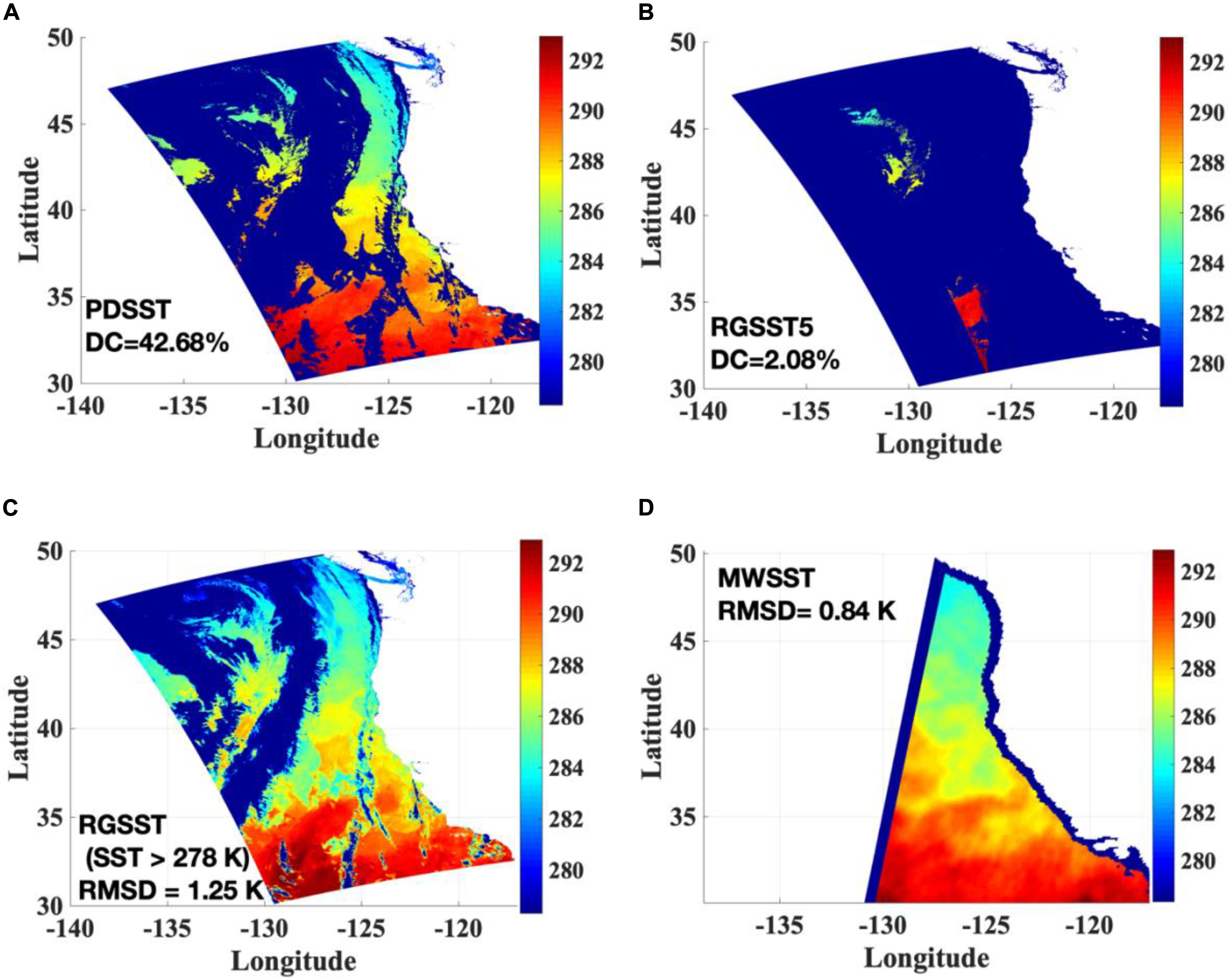
Figure 3. Comparison of daytime SST retrieval maps for California coast: (A) PDSST from MODIS-AQUA, (B) RGSST5 from MODIS-AQUA, (C) full-swath RGSST from MODIS-AQUA using a constraint of SST < 278 K, and (D) MW SST from AMSR2. DC stands for data coverage in percentage and RMSD is the root mean squared difference from matched in situ. The ranges of longitude and latitude from –180° to 180° and from –90° to 90° represent West to East and South to North, respectively. Unit of color bar is K. The color value of the darkest blue represents the Ocean portion.

The DC of RGSST from MODIS-AQUA increases to 5.74% (figure not shown) when QF is set to be ≥3, but is still very low as compared to the really cloud-free measurement of this granule (see Figure 3A). Reducing the value of QF even further (to QF ≥ 2) still does not show any increase in DC for this granule. Thus, all RGSSTs from the PO.DAAC database, with a constraint of the value of SST > 278 K, have been plotted in Figure 3C. This set of RGSST SSTs matched with 36 buoy measurements and the RMSD value is 1.25 K. The value of QF for PO.DAAC is 1 for all (36) matched locations. However, Figure 3C shows that most of the SSTs are comparable qualitatively (using the color map) with the same using PDSST. This implies that there is no relation between the value of QF and cloud-covered pixel. For example, it is hard to assume that the value QF = 1 means completely cloudy. From Figures 3A,C, it is clear that the obvious cloud pattern is easy to detect. The main difficulty is the detection of the fractional cloud, where RT-based tests using local atmospheric conditions in CEM play an important role. Once again, this implies that the RGSST from MODIS-AQUA product masked a large number of cloud-free SSTs using a low QF for the reduction of the overall error statistics of the end product. It can be concluded from this study that the physical model-based cloud detection scheme, CEM, is superior to the conventional threshold-based tests.

Although quantitative buoy validation for this granule is quite sufficient to prove the superiority of PDSST over RGSST from MODIS-AQUA, a qualitative comparison is introduced using MWSST from AMSR2 as is shown in Figure 3D. There are several granules at the operational level that never found any buoy matches despite the fact that the number of buoy measurements from iQuam is quite large. The qualitative comparison with MWSST may help to understand the quality of swath processed SSTs from PDSST when in situ are absent in a granule. There are several deficiencies of MWSST, namely low resolution (the nadir footprint is ∼25 km), radio-frequency interference, high retrieval error due to low signal strength of the Planck radiation, high wind-induced ocean surface emissivity, and the inability to retrieve temperatures near the coast (due to sidelobe contamination). The choice of MWSST for the qualitative validation (comparative color-map) is due to the following reasons: (a) there are very few absorption lines in the MW bands and the atmospheric transmission is significantly higher than the same of Infrared (IR) bands, which reduces the regression error, (b) MWSST is free from the ambiguities of cloud detection error.

Twenty-nine buoy matches are found from the MWSSTs for the region of Figure 3D, however, 26 of them are masked by QF = 1 due to land contamination as the distance from the coast is less than 40 km. This is a drawback for satellite-derived MWSSTs as the error in near-coast SSTs is high, however, SSTs from the dynamic coastal areas are highly important for many geophysical models. The RMSD is 0.84 K using only 3 buoy matches, which is more than double than the same for PDSST. Note that the value of RMSD is 7.81 K using 28 buoy matches when near-coast SSTs are included. This implies that the information content of SSTs from IR sensors is significantly higher than MWSSTs.

Note, MWSST from AMSR2 cannot be treated as a reference as: (a) it is a satellite-derived product with comparatively higher error than IR SST, (b) MODIS-AQUA and AMSR2 are not in the same satellite and there is some time difference, and (c) MWSST is not strictly a skin SST due to having different measurement physics. However, MWSSTs can be used to validate the performance of the cloud detection algorithm. As Figures 3A,D are in good agreement as per the color-map which confirmed that the cloud detection scheme in PDSST-suite is working well.

PDSST for Oceanic Fronts’ Study

Ocean fronts are one of the most important factors in several oceanic science developments. Ocean fronts are different in nature with respect to time and space, e.g., some large scale oceanic fronts extend down to thousands of meters and persevere for several months whereas microscale turbulence stretches up to a few meters and dissolves within minutes (for example, Bouali et al., 2017). These fronts should be visible through satellite-derived SST products and the California coast is well suited for this study as a dynamic oceanographic region (Vazquez-Cuervo et al., 2020).

To illustrate the strength of PDSST in the subject of Oceanic fronts’ study, the comparative results for a subset (9° by 8°) of granule − 3 (December 6, 2017) from Table 2 are plotted in Figure 4. This granule has been chosen carefully from a sunny day. PDSST in Figure 4A shows that level-2 SST from a granule is capable of extracting various oceanic features without any other manipulation. As a first-order validation of granule − 3 from Table 2, the RMSD value of PDSST is 0.34 K, by 31 cloud-free buoys, whereas the same for RGSST5 is 0.82 K, using only 2 cloud-free buoys. The RMSD value of PDSST is 0.28 K using 26 buoy matches for the selected subset (9° by 80°). This implies that PDSST outperforms RGSST5.

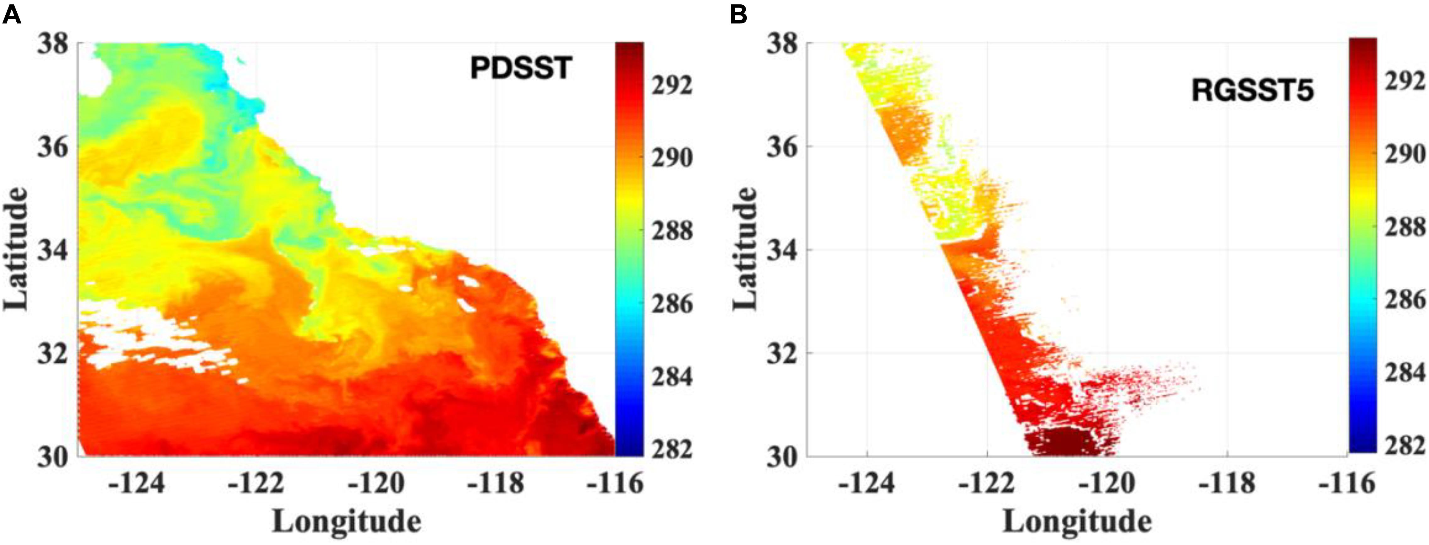
Figure 4. Comparison of daytime SST retrieval maps of a subset of area 9° by 8°from a granule of MODIS-AQUA for the California coast: (A) PDSST and (B) RGSST5. The ranges of longitude and latitude from −180° to 180° and from −90° to 90° represent West to East and South to North, respectively. Unit of color bar is K.

Note that the percentage of cloud-free pixels over the total pixels of the water body for the complete granule is ∼67.5% using PDSST and ∼16% using RGSST5. The DC of PDSST is almost 4 times more than that of RGSST5. Interestingly, the mean value of swath processed SSTs using the PDSST suite is ∼0.7 K colder than that of RGSST5 SSTs from the matched pixels of the two products (Figure not shown). PDSST algorithm uses the MWIR channels in its retrieval and is expected to be warmer than RGSST5 due to the high error in the visible components of the fast forward model.

To obtain more confidence in the quality of PDSST, the map of MWSST for the same day and location is also plotted in Figure 5A. Although it is not an apples-to-apples comparison, MWSST mapping (Figure 5A) endorses the assertion that PDSST (Figure 4A) is more accurate in detecting cloud-free pixels than the same for RGSST5 (Figure 4B). The statistics of MWSSTs for this granule are as follows: only 17 buoy measurements, out of 37, are matched with the non-zero SSTs from the MWSST product for the region of Figure 4A. However, 15 of them are masked by QF = 1 due to land contamination and the value of RMSD from 2 buoys is 0.77 K, which is more than double than the same from PDSST (0.37 K using 31 buoys).

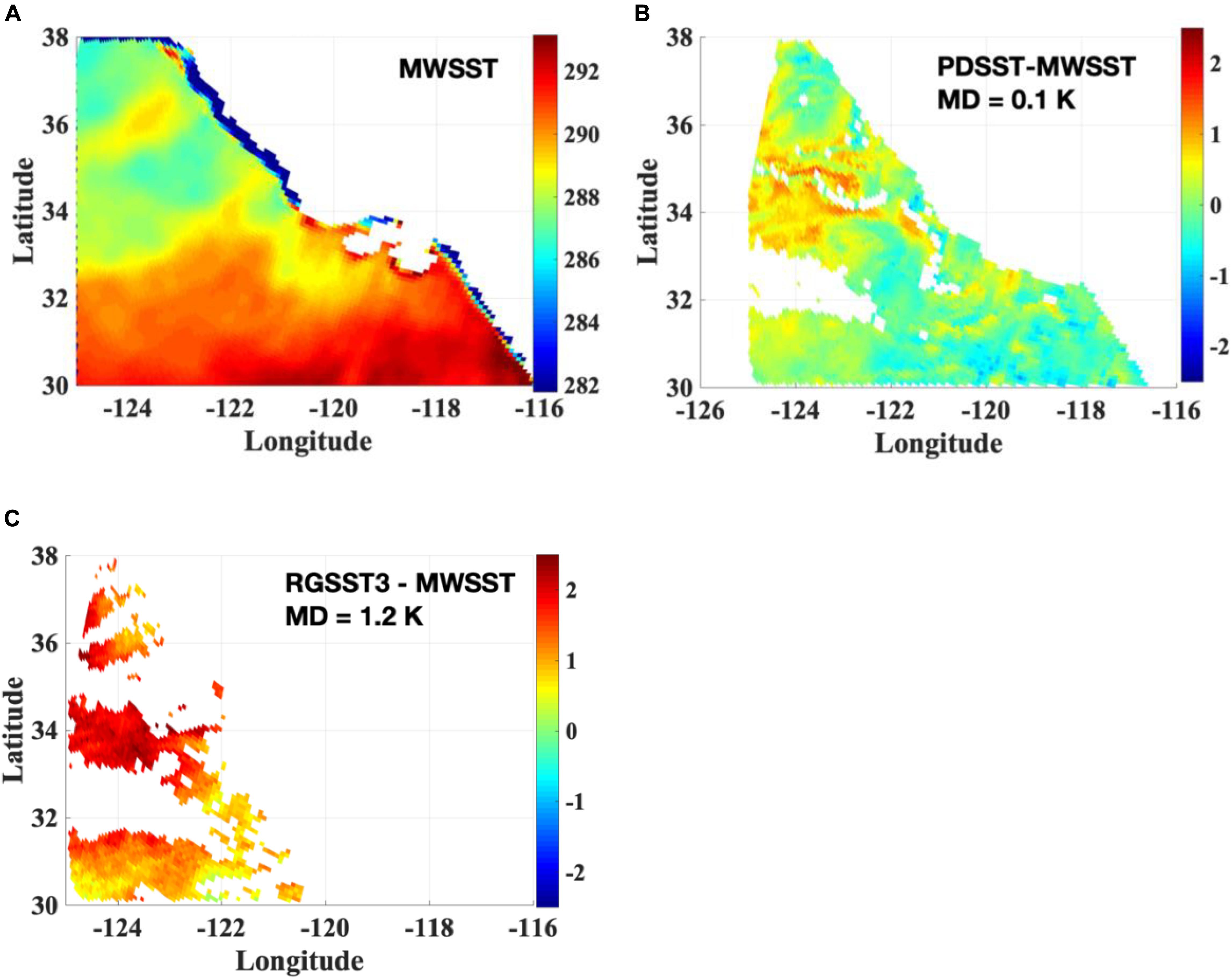
Figure 5. SSTs map for the same area of California coast as in Figure 4. (A) MWSST from AMSR2, (B) PDSST-MWSST, and (C) RGSST3-MWSST. MD stands for mean differences. The ranges of longitude and latitude from −180° to 180° and from –90° to 90° represent West to East and South to North, respectively. Unit of color bar in K.

To obtain more pixels and fewer gaps, the values of RGSST3 of the same granule (Figure 4B) are considered in the following study. The DC of RGSST3 for a full swath of the said granule increased to 34.6% from 16% (RGSST5). The RMSD value of RGSST3 is 0.82 K using 2 matched buoys, the same as of RGSST5. Both PDSST and RGSST3 for the above-mentioned subset of this granule are downscaled to the spatial resolution of MWSST and differences from MWSST are plotted in Figures 5B,C, respectively. Figure 5C shows that the average value of RGSSTs from MODIS-AQUA is 1.2 K higher than the same from MWSST product, whereas the mean difference of SSTs between PDSST and MWSST is 0.1 K (Figure 5B). It can be concluded from these comparison studies that RGSST from MODIS-AQUA is overestimating the SST values for the said CC area.

Another study is conducted to illustrate the validation of PDSST by comparing with other prevalent products of RGSST from MODIS-AQUA and MWSSTs from AMSR2SSTs from a subset (10° by 5°) of one granule from the same month (2nd December 2017) over the BB (granule – 2 from Table 4), since it is well known that in situ measurements in BB are sparse. Figures 6A,B show the results of PDSST-suite and RGSST5, respectively. There is only one buoy match found in this granule for quantitative validation. Note that the percentage of cloud-free pixels over the total pixels of the water body for the complete granule is 38.9% using PDSST and 17.5% using RGSST5. Figure 6A also shows that the DC of PDSST is 69.7%, whereas the DC for RGSST5 is 22.4% (Figure 6B) for the selected region, which is three times lower than that of PDSST.

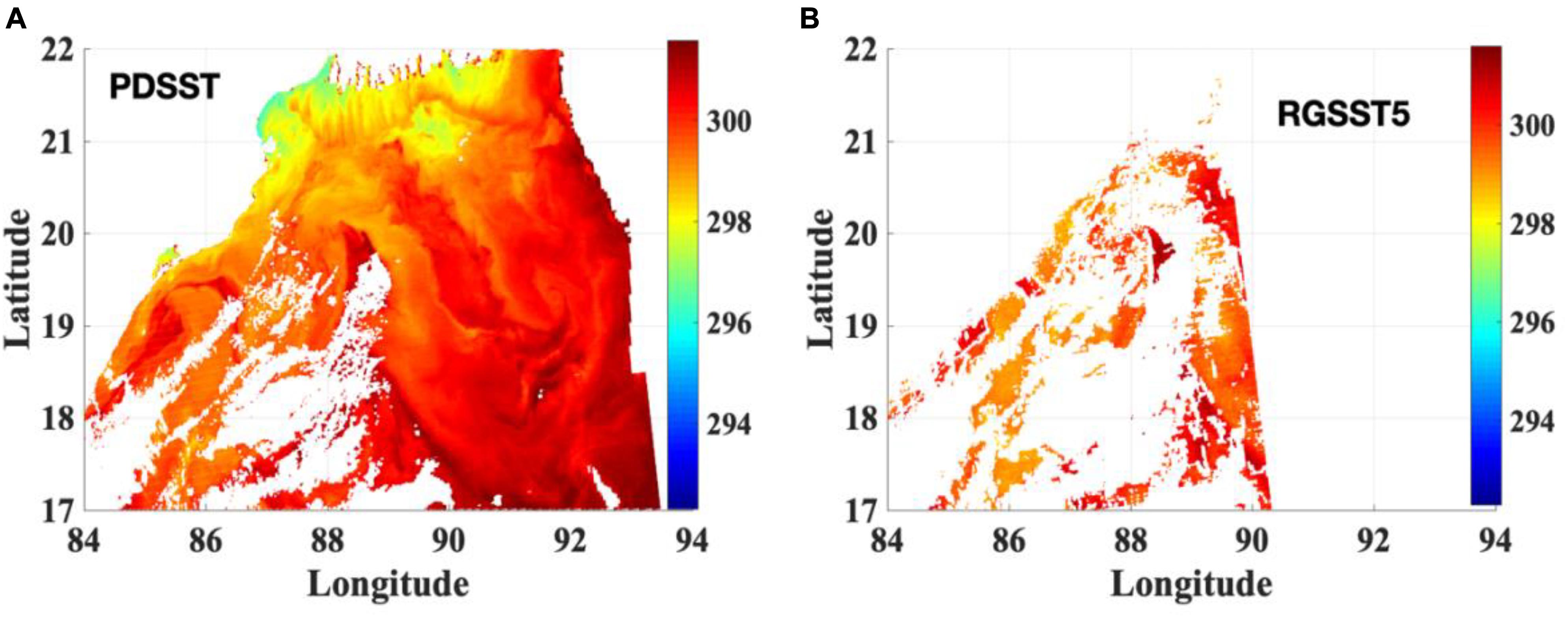
Figure 6. Comparison of daytime SST retrieval maps of a subset of area 10° by 5° from a granule of MODIS-AQUA for Bay of Bengal: (A) PDSST and (B) RGSST5. The ranges of longitude and latitude from −180° to 180° and from −90° to 90° represent West to East and South to North, respectively. Unit of color bar is K.

Similarly, the MWSSTs from AMSR2 for the selected region (as in Figure 6A) are plotted in Figure 7A. The satellite-derived SSTs in Figures 6A, 7A are harmonized on the matched region as similar to the previous case study of CC. This implies that there is no artifact in the PDSST retrieval scheme in terms of geographical locations.

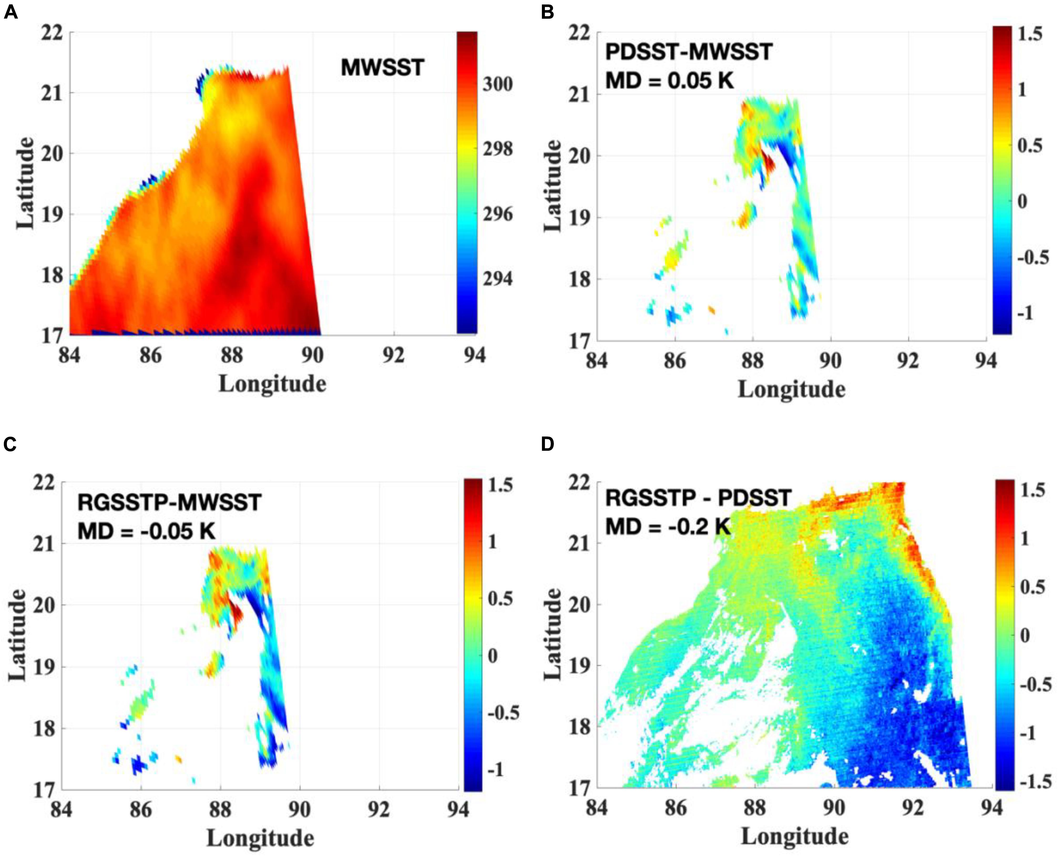
Figure 7. SST retrieval maps for the same subset as in Figure 6A. (A) MWSST from AMSR2, (B) Difference between PDSST and MWSST, (C) Difference between RGSSTP and MWSST, and (D) RGSSTP – PDSST. The ranges of longitude and latitude from −180° to 180° and from −90° to 90° represent West to East and South to North, respectively. Unit of color bar is K.

Even if the QF is reduced until 3, there are very few match points between RGSST3 and MWSST for the selected region (Figures 6A,B), making it difficult to produce conclusive results. Thus, a subset of RGSSTs from MODIS-AQUA, RGSSTP, is obtained using the cloud-free pixels according to the PDSST-suite for the following comparison study. Both PDSST and RGSSTP are re-gridded to the MWSST grid and differences from MWSST are plotted in Figures 7B,C, respectively. Figures 7B,C are qualitatively comparable, which implies that the quality of PDSST, including the MWIR channels, is as good as RGSST from MODIS-AQUA, without MWIR channels, under PDSST cloud-free subset for this region. However, PDSST cloud-free subset can extract 3 times more SST information as compared to the same for RGSST5. Such a comparative study may help to evaluate product quality when in situ measurements are hard to get for quantitative validation.

As can be seen from Figures 7B,C, the matched pixels between IR SST and MWSST are still infrequent and limited because the swaths are not matched due to being from different satellites and no SSTs are available beyond the satellite zenith angle of 55° for MWSST database. Thus, the differences between RGSSTP and PDSST are plotted in Figure 7D. A large number of retrievals from RGSSTP and PDSST are compared in Figure 7D. It is observed that the QF values of 48% pixels of the selected RGSSTP are 1, where the QF values are 5 for 38% of total matched pixels. On the other hand, all pixels for the said subset are cloud-free according to PDSST-suite. Once again, there is no correlation between the QF values from the RGSST product and realistic cloud-free conditions.

Results and Discussion

Physical Deterministic Sea Surface Temperature can provide at least 3 times more satellite-derived SST information by increasing DC and reducing the RMSD from in situ than RGSST5 according to the results are shown in Tables 1–5. Noticeably, the number of matched buoys from MC is 146 only, which is significantly lower than the same from CC and CB. The DC of RGSST5 for MC is higher than the same for CC and the value of information gain of PDSST over RGSST5 is low. This implies that the QF procedure for RGSST5 is more stringent for coastal areas because the set of granules for MC is from the deeper parts of the ocean than the same for CC. Also, the RMSD values for PDSST and RGSST5 are lower for MC than the same for CC, because the type of all buoys for MC is “drifter” whereas most of the buoys in CC are “coastal moored.”

The interesting result from the study of 98 granules from all Tables from three different regions is that the DC from PDSST for all granules is never less than the same from RGSST5. However, the RMSD values of PDSST for some granules are higher than the same from RGSST5. This occurs due to two reasons: (a) uneven sample size between PDSST and RGSST5, and (b) skin-bulk physics. The low RMSD values of RGSST5 from a granule are observed when the RMSD of PDSST is calculated from a significantly higher number of buoy measurements as compared to the same for RGSST5. For example, granule-3 of Table 1, where the RMSD of PDSST is 0.37 K using 27 matches whereas the RMSD of RGSST5 is 0.17 K using only 2 matches, which is questionable to calculate the statistics using a very low sample size. The satellite-derived SST is skin temperature and the buoy is located at ∼2 m depth of the ocean, and the validation of the satellite-derived SST against the bulk temperature of buoy is generally arguable (see details in Koner, 2020b). As alternative in situ databases for skin SST are not readily available, first-order validation of satellite-derived SSTs is accepted using buoy measurements. Moreover, RGSSTs are conventionally bulk SSTs due to the fact that regression coefficients are generated using bulk buoy measurements, whereas the PDSSTs are skin SSTs by definition (see details in Koner, 2020b).

Physical Deterministic Sea Surface Temperature is capable of fetching an enormous amount of valuable SST information as compared to the currently operational regression-based SST scheme for the dynamic oceanographic area of CC as per Figures 3A,B, 4A,B, 6A,B. One of the major reasons this has achieved such high information gain (∼20 times for a specific granule of Figures 4A,B) as compared to RGSST5 is that the PDSST suite uses more channels including MWIR channels and local atmospheric information from GFS data in daytime SST retrieval as well as for cloud detection scheme.

A sharp gradient for oceanic fronts using PDSST suite in CC and BB region is observed in Figures 4A, 6A, but the oceanic fronts almost disappeared in operational RGSST5 (Figures 4B, 6B). PDSST suite shows that the highest value of SST gradient magnitude is 1.36 K/pixel for CC and 2.24 K/pixel for BB. Some gradients of the SST fronts for the RGSST from MODIS-AQUA are visible if QF is set to be ≥3 (figure not shown) for BB, but not in CC. However, the sharp gradients are absent even for QF ≥ 3 as is seen in Figure 6A. A similar conclusion for BB is reported in a recent publication (Samanta et al., 2018).

Interestingly, PDSST result assures that the oceanic fronts and eddies of a dynamic oceanographic region can be studied using PDSST for a cloud-free region with a finer scale of ∼1 × 1 km (nadir viewing) grid box (Figures 4A, 6A), which was difficult using regression-based satellite IR SSTs (Figures 4B, 6B). Generally, oceanic fronts and eddies are studied using MWSST due to the fact that microwave measurement can penetrate clouds and produce gap-free SSTs. Moreover, the spatial resolution of MW SST is lower (∼25 × 25 km) than that of IR SST and also has a higher retrieval error (at least double than that of PDSST). Since PDSST declares ∼20−25% of global measurements as cloud-free (Koner and Harris, 2016b) and spatial resolution is ∼500 times higher, the information gain using PDSST will be of roughly two orders (∼10²) of magnitude as compared to MW SST. This will certainly be an avenue for enhancing the understanding of different oceanic science studies.

A noticeable deficiency of the regression-based SST retrieval scheme can be observed from Figures 6B, 7A, where no SST is retrieved beyond the longitude of ∼ 90°. SSTs are not retrieved using any regression-based methods if the satellite zenith angle of the measurement is more than 55° due to high error in SSTs. This also confirms that a large number of MWSSTs are discarded from healthy satellite measurements due to the choice of the applied retrieval algorithm.

Although the mean differences between PDSST and RGSSTP is −0.2 K for a particular granule (Figure 7D), 18 granules of December 2017 from BB have been studied and it is found that the average mean difference is ∼−0.5 K (results not shown). To illustrate more on this issue, a recent publication on “Nature” (Samanta et al., 2018) reports that Indian summer monsoon is modeled using satellite-derived SST data surrounded by the BB, but a bias of −0.5 K is removed from the observed SST data to facilitate the validation of the higher-level scientific model. This discrepancy is likely due to the used satellite-derived IR SST data being ambiguous.

The difference in SSTs between PDSST and RGSSTP varies from +1.5 K to −1.5 K for the region of BB as is seen in Figure 7D. It is observed from the retrieved TCWV using PDSST algorithm as shown in Figure 8 that the RGSSTs from MODIS-AQUA show an overestimate of ∼1.5 K for the region where TCWV quantity is ∼10 Kg/m² and an underestimate of ∼1.5 K where TCWV is higher (∼30 Kg/m²) as compared to the same for PDSST. A rigorous validation on the retrieved TCWV using PDSST will be conducted and reported in a future publication. However, this is an additional advantage of PDSST-suite that it can help to improve the quality and spatial resolution of TCWV data obtained from GFS model. Although the absorption of RT physics is dependent on the profile shape of water vapor, it is just a first-order estimate using TCWV to demonstrate the outcome. Since PDSST uses the local atmospheric conditions from GFS data, it is expected that the quality of SSTs from the PDSST-suite is better than RGSST, and the observed differences are probably the errors in RGSSTs.

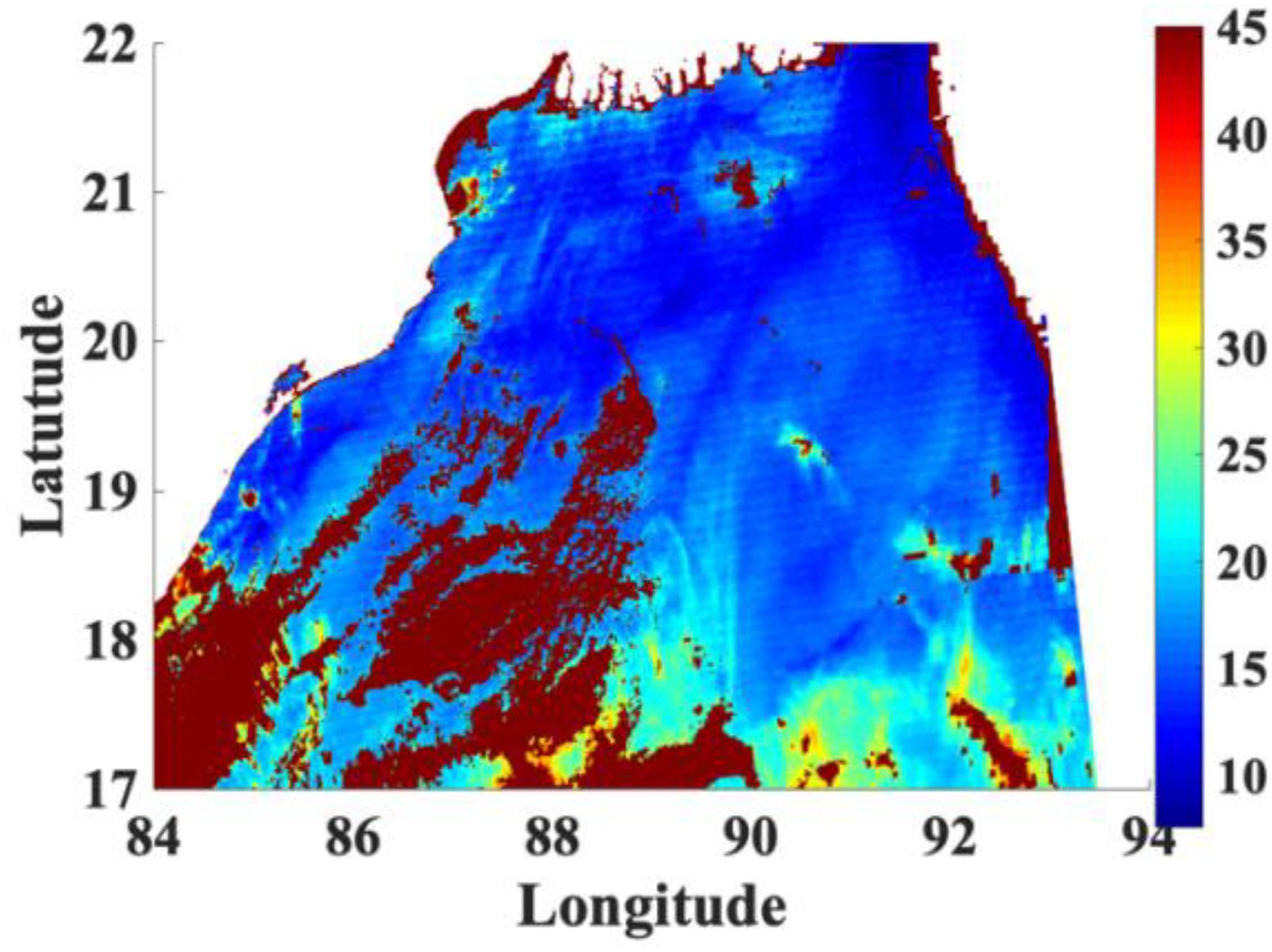
Figure 8. Retrieved TCWV maps using PDSST for the same subset as in Figure 6A. The ranges of longitude and latitude from −180° to 180° and from −90° to 90° represent West to East and South to North, respectively. Unit of color bar is kg/m². Dark brown color represents the “NaN” values.

It is not just the fact that one granule of CC shows 1.2 K bias from MWSST, the average bias of RGSST5 from MWSST for all 20 granules is 0.97 K. On the contrary, the bias of RGSST5 for BB from 18 granules is −0.5 K for the same months. The opposite sign of the regional bias can be discussed as the atmospheric condition of CC for the month of December is dry as compared to the same for BB. Additionally, BB has a high aerosol content as compared to the same for CC. Such different regional bias cannot be studied in global matchups’ study (see Koner, 2020b) because positive and negative regional biases are averaged out in the global statistics. A detailed study on the effects of TCWV and aerosols on RGSST5 at Somalia coast of IO has been already discussed in an earlier publication (Koner, 2019). On the contrary, such problems of TCWV and aerosol have no major effect on the PDSST retrieval because PDSST uses local atmospheric condition information through GFS data. Also, PDSST does not rely 100% on GFS data, and both TCWV and aerosols are in the retrieved vector of PDSST algorithm to correct the GFS data.

Conclusion

The swath-processed SSTs using the PDSST suite on MODIS-AQUA radiance data for coastal and near-coastal areas reveal that enhanced SST information can be obtained using MWIR channels in the daytime SST retrieval scheme. The information gain of PDSST over RGSST5 is even higher in the coastal areas of CC, CB, and BB as compared to the global matchup studies (Koner, 2020b). This is a paradigm shift in results of 3−5 times information gain over prevalent method. TCM study shows that true information gain of PDSST over RGSST5 for near-coastal areas (only drifter matchups) is more than double apart from the increased DC for PDSST. The SST information of coastal and dynamic oceanographic regions is highly valuable because this information is essential to enhance scientific models for atmospheric and oceanographic features, and the PDSST suite can play an important role.

Although the effects of increased satellite-derived SST information using PDSST on oceanic fronts’ study are demonstrated in this work, the increased information content of PDSST can help to better understand many oceanic science problems. This study confirms that the PDSST retrieval scheme can produce unambiguous SST retrieval from satellite measurements to open up a new frontier in oceanic science by increasing the coverage and resolution in space and time of high-quality observations. Additionally, the physical deterministic algorithm is generic and is found to be superior to other stochastic retrieval methods for profile retrieval using remote sensing empirical data (Koner and Drummond, 2008a,b; Koner et al., 2010, 2016a; Koner and Dash, 2018; Koner, 2020a). This work endorses that the transformative inverse approach of PDSST can maximize unambiguous quantitative information from realistic satellite remote sensing measurements.

Recommendations

Apart from this study, the nighttime SSTs using PDSST-suite have been already compared with the operational PO.DAAC SSTs in an earlier publication (Koner and Harris, 2016b) and PDSST-suite was found to have 2−3 times information gain. Large discrepancies of RGSST5 (MODIS SSTs) are observed with respect to the in situ measurements for daytime (Koner, 2020b), where the short-comings of the regression-based daytime SST retrievals using only two channels and without MWIR channel/s are thoroughly discussed. This is not the first time on record; several earlier publications (for example, Smale and Wernberg, 2009; Crosman and Horel, 2009; Castillo and Lima, 2010; Dufois et al., 2012; Smit et al., 2013; Bouali et al., 2017; Hao et al., 2017; Pimentel et al., 2019) reported the same. It is also shown in Koner (2020b) that daytime SST retrieval, including one MWIR channel, using another prevalent physical-based estimation method (cf. Masiello et al., 2015; Peres et al., 2017), where the error is being treated as definite information, is equally ambiguous. In observational science, measurement is the most important component to develop a scientific model. Higher-level scientific models will be imprecise when ambiguous satellite-derived parameters are used. For example, MODIS SSTs were used as the measurement for several oceanographic scientific models (e.g., Barré et al., 2006; Turiel et al., 2008; Knievel et al., 2010; Gawarkiewicz et al., 2012; Kozlov et al., 2012; Williams et al., 2013; Callies et al., 2015; Huang and Feng, 2015). Most of these studies require additional tweaking to the operational PO.DAAC MODIS SSTs to fetch some scientific information, but it is still questionable (e.g., Smit et al., 2013; Bouali et al., 2017) to develop a scientific model using such ambiguous data.

Operational SST retrieval from imager measurements using regression-based method is still dominating in this community. The SST product from MODIS-AQUA distributed by PO.DAAC is also using the regression-based method. Such approaches were justifiable in the interest of time and the lack of computational resources when they were formulated ∼4−5 decades ago. With the availability of improved computational facilities, the implementation of PDSST for the near-real-time operational environment is feasible (see Koner et al., 2015). Broadly, the regression-based stochastic inverse method can extract the qualitative information from the measurements to understand the problem at the early stages of scientific development, and the physical deterministic inverse is highly desirable to maximize the quantitative information from remote sensing measurements where a mature forward model exists. This is a call-to-action for the community to rethink the appropriate inverse method for operational SST retrieval from advanced imager measurements.

Data Availability Statement

The datasets presented in this article are not readily available due to large file sizes preventing data transfer through conventional means. Requests to access the datasets should be directed to pkoner@umd.edu.

Author Contributions

The author confirms being the sole contributor of this work and has approved it for publication.

Funding

This work was funded under NASA Grant number 80NSSC18K0705.

Conflict of Interest

The authors declare that the research was conducted in the absence of any commercial or financial relationships that could be construed as a potential conflict of interest.

Acknowledgments

The author thanks Dr. Andy Harris, University of Maryland for helpful discussions. The author acknowledges NASA (https://ladsweb.modaps.eosdis.nasa.gov/archive/allData/61/ and https://podaac-tools.jpl.nasa.gov/drive/files/allData/ghrsst/data/GDS2/L2P), NOAA (https://ftp.emc.ncep.noaa.gov/jcsda/CRTM/, https://www.star.nesdis.noaa.gov/socd/sst/iquam, and https://www.ncei.noaa.gov/data/global-forecast-system/access/grid-004-0.5-degree/forecast/), and RSS (ftp://ftp.remss.com/sst/misst/GDS2/L2P/AMSR2/REMSS/v8a) for making their data publicly available and Sravan Garimella, University of Maryland for the editing help.

References

Acha, E. M., Mianzan, H. W., Guerrero, R. A., Favero, M., and Bava, J. (2004). Marine fronts at the continental shelves of Austral South America. J. Mar. Syst. 44, 83–105. doi: 10.1016/j.jmarsys.2003.09.005
Barré, N., Provost, C., and Saraceno, M. (2006). Spatial and temporal scales of the Brazil–malvinas current confluence documented by simultaneous MODIS Aqua 1.1-Km Resolution SST and color images. Adv. Space Res. 37, 770–786. doi: 10.1016/j.asr.2005.09.026
Behrenfeld, M. J., and Falkowski, P. G. (1997). Photosynthetic rates derived from satellite-based chlorophyll concentration. Limnol. Oceanogr. 42, 1–20. doi: 10.4319/lo.1997.42.1.0001
Behrenfeld, M. J., O’Malley, R. T., Siegel, D. A., Mcclain, C. R., Sarmiento, J. L., Feldman, G. C., et al. (2006). Climate-driven trends in contemporary ocean productivity. Nature 444, 752–755. doi: 10.1038/nature05317
Bentamy, A., Piollé, J. F., Grouazel, A., Danielson, R., Gulev, S., Paul, F., et al. (2017). Review and assessment of latent and sensible heat flux accuracy over the global Oceans. Remote Sens. Environ. 201, 196–218. doi: 10.1016/j.rse.2017.08.016
Bouali, M., Sato, O. T., and Polito, P. S. (2017). Temporal trends in sea surface temperature gradients in the South Atlantic Ocean. Remote Sens. Environ. 194, 100–114. doi: 10.1016/j.rse.2017.03.008
Callies, J., Ferrari, R., Klymak, J. M., and Gula, J. (2015). Seasonality in submesoscale turbulence. Nat. Commun. 6, 1–8. doi: 10.1038/ncomms7862
Castillo, K. D., and Lima, F. P. (2010). Comparison of in situ and satellite-derived (MODIS-Aqua/Terra) methods for assessing temperatures on Coral Reefs. Limnol. Oceanogr. 8, 107–117. doi: 10.4319/lom.2010.8.0107
Chatterjee, A., Kumar, B. P., Prakash, S., and Singh, P. (2019). Annihilation of the somali upwelling system during summer Monsoon. Sci. Rep. 9:7598. doi: 10.1038/s41598-019-44099-1
Crosman, E. T., and Horel, J. D. (2009). MODIS-derived surface temperature of the great salt lake. Remote Sens. Environ. 113, 73–81. doi: 10.1016/j.rse.2008.08.013
Dong, B., Dai, A., Vuille, M., and Timm, O. E. (2018). Asymmetric modulation of ENSO teleconnections by the interdecadal Pacific Oscillation. J. Clim. 31, 7337–7361. doi: 10.1175/jcli-d-17-0663.1
Dufois, F., Penven, P., Whittle, C. P., and Veitch, J. (2012). On the warm nearshore bias in pathfinder monthly SST products over eastern boundary upwelling systems. Ocean Model. 47, 113–118. doi: 10.1016/j.ocemod.2012.01.007
Dufois, F., and Rouault, M. (2012). Sea surface temperature in false bay (South Africa): towards a better understanding of its seasonal and inter-annual variability. Cont. Shelf Res. 43, 24–35. doi: 10.1016/j.csr.2012.04.009
Fèvre, J. L. (1987). Aspects of the biology of frontal systems. Adv. Mar. Biol. 23, 163–299. doi: 10.1016/s0065-2881(08)60109-1
Gawarkiewicz, G. G., Todd, R. E., Plueddemann, A. J., Andres, M., and Manning, J. P. (2012). Direct Interaction between the gulf stream and the shelfbreak South of New England. Sci. Rep. 2:553. doi: 10.1038/srep00553
Hao, Y., Cui, T., Singh, V. P., Zhang, J., Yu, R., and Zhang, Z. (2017). Validation of MODIS sea surface temperature product in the coastal waters of the Yellow Sea. IEEE J. Select. Top. Appl. Earth Observ. Remote Sens. 10, 1667–1680. doi: 10.1109/jstars.2017.2651951
Huang, Z., and Feng, M. (2015). Remotely sensed spatial and temporal variability of the leeuwin current using MODIS Data. Remote Sens. Environ. 166, 214–232. doi: 10.1016/j.rse.2015.05.028
Jha, B., Hu, Z., and Kumar, A. (2013). SST and ENSO variability and change simulated in historical experiments of CMIP5 models. Clim. Dyn. 42, 2113–2124. doi: 10.1007/s00382-013-1803-z
Knievel, J. C., Rife, D. L., Grim, J. A., Hahmann, A. N., Hacker, J. P., Ge, M., et al. (2010). A simple technique for creating regional composites of sea surface temperature from MODIS for Use in Operational Mesoscale NWP. J. Appl. Meteorol. Climatol. 49, 2267–2284. doi: 10.1175/2010jamc2430.1
Koner, P. K. (2018). Physical deterministic sea surface temperature retrieval suite for satellite infrared measurement. Adv. Sensor Rev. 5, 497–530.
Koner, P. K. (2019). “Daytime sea surface temperature retrieval using shortwave infrared channel(s),” in Processing of the SPIE 11150, Remote Sensing of the Ocean, Sea Ice, Coastal Waters, and Large Water Regions, Strasbourg, doi: 10.1117/12.2532817
Koner, P. K. (2020a). A transformative approach to enhance the parameter information from microwave and infrared remote sensing measurements. Big Earth Data doi: 10.1080/20964471.2020.1776435 [Epub ahead of print].
Koner, P. K. (2020b). “Daytime sea surface temperature retrieval incorporating mid-wave imager measurements: algorithm development and validation,” in IEEE Transactions on Geoscience and Remote Sensing, Piscataway, NJ: IEEE, doi: 10.1109/TGRS.2020.3008656
Koner, P. K., Battaglia, A., and Simmer, C. (2010). A rain-rate retrieval algorithm for attenuated radar measurements. J. Appl. Meteorol. Climatol. 49, 381–393. doi: 10.1175/2009jamc2279.1
Koner, P. K., and Dash, P. (2018). Maximizing the information content of Ill-posed space-based measurements using deterministic inverse method. Remote Sens. 10:994. doi: 10.3390/rs10070994
Koner, P. K., and Drummond, J. R. (2008a). A comparison of regularization techniques for atmospheric trace gases retrievals. J. Q. Spectrosc. Radiat. Trans. 109, 514–526. doi: 10.1016/j.jqsrt.2007.07.018
Koner, P. K., and Drummond, J. R. (2008b). Atmospheric trace gases profile retrievals using the nonlinear regularized total least squares method. J. Q. Spectros. Radiat. Trans. 109, 2045–2059. doi: 10.1016/j.jqsrt.2008.02.014
Koner, P. K., and Harris, A. (2016a). Improved quality of MODIS Sea surface temperature retrieval and data coverage using physical deterministic methods. Remote Sens. 8:454. doi: 10.3390/rs8060454
Koner, P. K., and Harris, A. (2016b). Sea surface temperature retrieval from MODIS radiances using truncated total least squares with multiple channels and parameters. Remote Sens. 8:725. doi: 10.3390/rs8090725
Koner, P. K., Harris, A., and Maturi, E. (2015). A physical deterministic inverse method for operational satellite remote sensing: an application for sea surface temperature retrievals. IEEE Trans. Geosci. Remote Sens. 53, 5872–5888. doi: 10.1109/tgrs.2015.2424219
Koner, P. K., Harris, A. R., and Dash, P. (2016a). A deterministic method for profile retrievals from hyperspectral satellite measurements. IEEE Trans. Geosci. Remote Sens. 54, 5657–5670. doi: 10.1109/tgrs.2016.2565722
Koner, P. K., Harris, A., and Maturi, E. (2016b). Hybrid cloud and error masking to improve the quality of deterministic satellite sea surface temperature retrieval and data coverage. Remote Sens. Environ. 174, 266–278. doi: 10.1016/j.rse.2015.12.015
Kozlov, I. E., Kudryavtsev, V. N., Johannessen, J. A., Chapron, B., Dailidienë, I., and Myasoedov, A. G. (2012). ASAR imaging for coastal upwelling in the Baltic Sea. Adv. Space Res. 50, 1125–1137. doi: 10.1016/j.asr.2011.08.017
Largier, J. L. (1993). Estuarine fronts: how important are they? Estuaries 16, 1–11. doi: 10.2307/1352760
Lorenzo, E. D., and Mantua, N. (2016). Multi-year persistence of the 2014/15 North Pacific marine Heatwave. Nat. Clim. Change 6, 1042–1047. doi: 10.1038/nclimate3082
Masiello, G., Serio, C., Venafra, S., Liuzzi, G., Göttsche, F., Trigo, I. F., et al. (2015). Kalman filter physical retrieval of surface emissivity and temperature from SEVIRI infrared channels: a validation and intercomparison study. Atmosph. Meas. Tech. 8, 2981–2997. doi: 10.5194/amt-8-2981-2015
Mcphaden, M. J., Zhang, X., Hendon, H. H., and Wheeler, M. C. (2006). Large scale dynamics and MJO forcing of ENSO variability. Geophys. Res. Lett. 33:L16702. doi: 10.1029/2006gl026786
Minobe, S., Kuwano-Yoshida, A., Komori, N., Xie, S., and Small, R. J. (2008). Influence of the gulf stream on the troposphere. Nature 452, 206–209. doi: 10.1038/nature06690
O’Neill, L. W., Esbensen, S. K., Thum, N., Samelson, R. M., and Chelton, D. B. (2010). Dynamical analysis of the boundary layer and surface wind responses to mesoscale SST perturbations. J. Clim. 23, 559–581. doi: 10.1175/2009jcli2662.1
Peres, L. F., Franca, G. B., Paes, R. C. O. V., Sousa, R. C., and Oliveira, A. N. (2017). Analyses of the positive bias of remotely sensed SST retrievals in the coastal waters of Rio De Janeiro. IEEE Trans. Geosci. Remote Sens. 55, 6344–6353. doi: 10.1109/tgrs.2017.2726344
Perlin, N., De Szoeke, S. P., Chelton, D. B., Samelson, R. M., Skyllingstad, E. D., and O’Neill, L. W. (2014). Modeling the atmospheric boundary layer wind response to mesoscale sea surface temperature perturbations. Month. Weather Rev. 142, 4284–4307. doi: 10.1175/mwr-d-13-00332.1
Pimentel, G. R., Franca, G. B., and Peres, L. F. (2019). Removal of the MCSST MODIS SST bias during upwelling events along the Southeastern Coast of Brazil. IEEE Trans. Geoscie. Remote Sens. 57, 3566–3573. doi: 10.1109/tgrs.2018.2885759
Preston, B. L. (2004). Observed winter warming of the chesapeake bay estuary (1949–2002): implications for ecosystem management. Environ. Manag. 34, 125–139. doi: 10.1007/s00267-004-0159-x
Rivas, A. L., and Pisoni, J. P. (2010). Identification, characteristics and seasonal evolution of surface thermal fronts in the argentinean Continental Shelf. J. Mar. Syst. 79, 134–143. doi: 10.1016/j.jmarsys.2009.07.008
Samanta, D., Hameed, S. N., Jin, D., Thilakan, V., Ganai, M., Rao, S. A., et al. (2018). Impact of a narrow coastal bay of bengal sea surface temperature front on an Indian Summer Monsoon simulation. Sci. Rep. 8:17694. doi: 10.1038/s41598-018-35735-3
Santos, A. M. P. (2000). Fisheries oceanography using satellite and airborne remote sensing methods: a review. Fish. Res. 49, 1–20. doi: 10.1016/s0165-7836(00)00201-0
Saraceno, M., Provost, C., and Piola, A. R. (2005). On the relationship between satellite-retrieved surface temperature fronts and chlorophyllain the Western South Atlantic. J. Geophys. Res. 110:C11016. doi: 10.1029/2004jc002736
Sirjacobs, D., Alvera-Azcárate, A., Barth, A., Lacroix, G., Park, Y., Nechad, B., et al. (2011). Cloud filling of ocean colour and sea surface temperature remote sensing products over the southern north sea by the data interpolating empirical orthogonal functions methodology. J. Sea Res. 65, 114–130. doi: 10.1016/j.seares.2010.08.002
Smale, D., and Wernberg, T. (2009). Satellite-derived SST data as a proxy for water temperature in nearshore benthic ecology. Mar. Ecol. Prog. Ser. 387, 27–37. doi: 10.3354/meps08132
Smit, A. J., Roberts, M., Anderson, R. J., Dufois, F., Dudley, S. F. J., Bornman, T. G., et al. (2013). A coastal seawater temperature dataset for biogeographical studies: large biases between in situ and remotely-sensed data sets around the Coast of South Africa. PLoS One 8:e0081944. doi: 10.1371/journal.pone.0081944
Stoffelen, A. (1998). Toward the true near-surface wind speed: error modeling and calibration using triple collocation. J. Geophys. Res. 103, 7755–7766. doi: 10.1029/97jc03180
Tandeo, P., Chapron, B., Ba, S., Autret, E., and Fablet, R. (2014). Segmentation of mesoscale ocean surface dynamics using satellite SST and SSH observations. IEEE Trans. Geosci. Remote Sens. 52, 4227–4235. doi: 10.1109/tgrs.2013.2280494
Turiel, A., Solé, J., Nieves, V., Ballabrera-Poy, J., and García-Ladona, E. (2008). Tracking oceanic currents by singularity analysis of microwave sea surface temperature images. Remote Sens. Environ. 112, 2246–2260. doi: 10.1016/j.rse.2007.10.007
Vazquez-Cuervo, J., Gomez-Valdes, J., and Bouali, M. (2020). Comparison of satellite- derived sea surface temperature and sea surface salinity gradients using the Saildrone California/Baja and North Atlantic Gulf stream deployments. Remote Sen. 12:1839. doi: 10.3390/rs12111839
Wanninkhof, R., Asher, W. E., Ho, D. T., Sweeney, C., and Mcgillis, W. R. (2009). Advances in quantifying air-sea gas exchange and environmental forcing. Annu. Rev. Mar. Sci. 1, 213–244. doi: 10.1146/annurev.marine.010908.163742
Williams, G. N., Dogliotti, A. I., Zaidman, P., Solis, M., Narvarte, M. A., González, R. C., et al. (2013). Assessment of remotely-sensed sea-surface temperature and chlorophyll-a concentration in san matías gulf (Patagonia. Argentina). Cont. Shelf Res. 52, 159–171. doi: 10.1016/j.csr.2012.08.014
Xu, F., and Ignatov, A. (2014). In Situ SST quality monitor (IQuam). J. Atmos. Oceanic Technol. 31, 164–180. doi: 10.1175/jtech-d-13-00121.1
Zainuddin, M., Kiyofuji, H., Saitoh, K., and Saitoh, S. (2006). Using multi-sensor satellite remote sensing and catch data to detect ocean hot spots for albacore (Thunnus Alalunga) in the Northwestern North Pacific. Deep Sea Res. Part II Top. Stud. Oceanogr. 53, 419–431. doi: 10.1016/j.dsr2.2006.01.007
Keywords: infrared image sensors (MODIS-AQUA), information retrieval, inverse problem (physical deterministic), microwave sensor (AMSR2), remote sensing, radiative transfer, sea surface temperature
Citation: Koner PK (2020) Enhancing Information Content in the Satellite-Derived Daytime Infrared Sea Surface Temperature Dataset Using a Transformative Approach. Front. Mar. Sci. 7:556626. doi: 10.3389/fmars.2020.556626
Received: 28 April 2020; Accepted: 27 August 2020;
Published: 25 September 2020.
Edited by:
Agustin Sanchez-Arcilla, Universitat Politecnica de Catalunya, SpainReviewed by:
José Pinho, University of Minho, PortugalJorge Vazquez, NASA Jet Propulsion Laboratory, United States
Copyright © 2020 Koner. This is an open-access article distributed under the terms of the Creative Commons Attribution License (CC BY). The use, distribution or reproduction in other forums is permitted, provided the original author(s) and the copyright owner(s) are credited and that the original publication in this journal is cited, in accordance with accepted academic practice. No use, distribution or reproduction is permitted which does not comply with these terms.
*Correspondence: Prabhat K. Koner, pkoner@umd.edu