Extremal Trees with Respect to the Difference between Atom-Bond Connectivity Index and Randić Index


1
Faculty of Ocean Engineering Technology and Informatics, Universiti Malaysia Terengganu, Kuala Nerus 21030, Terengganu, Malaysia
2
School of Software, South China Normal University, Foshan 528225, China
3
School of Mathematics and Statistics, Zhaoqing University, Zhaoqing 526061, China
4
Department of Mathematics, Riphah Institute of Computing and Applied Sciences, Riphah International University, Lahore 46000, Pakistan
*
Author to whom correspondence should be addressed.
Symmetry 2020, 12(10), 1591; https://doi.org/10.3390/sym12101591
Submission received: 23 July 2020
/
Revised: 20 August 2020
/
Accepted: 23 August 2020
/
Published: 25 September 2020
(This article belongs to the Special Issue Analytical and Computational Properties of Topological Indices)
Abstract
:Let G be a simple, connected and undirected graph. The atom-bond connectivity index () and Randić index () are the two most well known topological indices. Recently, Ali and Du (2017) introduced the difference between atom-bond connectivity and Randić indices, denoted as index. In this paper, we determine the fourth, the fifth and the sixth maximum chemical trees values of for chemical trees, and characterize the corresponding extremal graphs. We also obtain an upper bound for index of such trees with given number of pendant vertices. The role of symmetry has great importance in different areas of graph theory especially in chemical graph theory.
1. Introduction
Let G be a simple, connected and undirected graph. having and as the set of vertices and edges respectively. The number of vertices and edges in G are denoted by n m, respectively. Let denotes the degree of vertex u in G, while and are used to denote the maximum and minimum degree of G. The distance between vertices x and y is defined as the length of any shortest path in G connecting x and y. The eccentricity of in G is defined as . For more concepts and terminologies in Graph Theory, we refer to [1].
Topological indices is one of the useful tools of graph theory [2]. Molecular compounds are often modeled by molecular graphs are used to represent the molecules and molecular compounds with the help of lines and dots. In study of QSPR/QSAR, topological indices are considered as one of the useful topics [3].
In 1975, Randić [4] defined the Randić index as follows:
Estrada et al. [11] proposed the atom-bond connectivity ( for short) for a molecular graph as
This index became popular only ten years later, when the paper [12] was published. For the details, see the surveys [13], the recent papers [14,15,16,17,18,19] and the references cited therein.
Nowadays, studying the relationship or comparison between topological indices, see [20,21,22,23], is becoming popular. Recently, Ali and Du [24] investigated extremal binary and chemical trees results for the difference between and R indices. A tree with maximum degree at most three or four called a binary and chemical tree, respectively.
For a connected graph G of order at least 3, the difference between and R is represented as (see [24])
Note that and equality holds if and only if . So in our discussion we consider .
2. Preliminary Results
Let the number of edges connecting the vertices of degree p and q is denoted by . In term of and can be rewritten as follows [24]:
Let be the number of vertices of degree p in G, where . Then for any n-vertex chemical tree the following system of equations holds (see [19,24]):
From Equations (2) and (3), it follows that
and thus,
By solving the sysmtem of Equations (2)–(7), the values of and are, respectively, given as below (see also Refs. [24,26]):
Note that the detailed calculation of obtaining the values for and can be referred in [26].
By substituting these values of and in Equation (1), one has:
Let
From Equation (12) we have . Moreover Equation (11) implies that a chemical tree which gives the minimum value of will produce the maximum of .
Theorem 1
([24]). Consider the set of all n-vertex chemical trees.
- (1)
- Suppose that .
- (1.1)
- For , the maximum value iswhich is uniquely attained by those trees that contain a unique vertex of degree 2 and no vertex of degree 3, that is, and , such that the unique vertex of degree 2 is adjacent to two vertices of degree 4, that is, and .
- (1.2)
- For , the second maximum value iswhich is uniquely attained by those trees that contain no vertex of degree 2 and exactly two vertices of degree 3, that is, and , such that each vertex of degree 3 is adjacent to three vertices of degree 4, that is, and .
- (1.3)
- For , the third maximum value iswhich is uniquely attained by those trees that contain no vertex of degree 2 and exactly two vertices of degree 3, which are adjacent, that is, , , and such that each vertex of degree 3 is adjacent to exactly two vertices of degree 4, that is, and .
- (2)
- Suppose that .
- (2.1)
- For , the maximum value isand the equality holds if and only if and such that and .
- (2.2)
- For , the second maximum value iswhich is uniquely attained by those trees that contain exactly two vertices of degree 2 and no vertex of degree 3, that is, and , such that either vertex of degree 2 is adjacent to two vertices of degree 4, that is, and .
- (2.3)
- For , the third maximum value iswhich is uniquely attained by those trees that contain a unique vertex of degree 2 and exactly two vertices of degree 3, that is, and , such that each vertex of degree 2 and 3 is adjacent to only vertices of degree 4, that is, , , and .
- (3)
- Suppose that .
- (3.1)
- For , the maximum value iswhich is uniquely attained by those trees that contain no vertex of degree 2 or 3, that is, .
- (3.2)
- For , the second maximum value iswhich is uniquely attained by those trees that contain a unique vertex of degree 2 and a unique vertex of degree 3, that is, , such that each vertex of degree 2 and 3 is adjacent to only vertices of degree 4, that is, , , and .
- (3.3)
- For , the third maximum value iswhich is uniquely attained by those trees that contain no vertex of degree 2 and exactly three vertices of degree 3, that is, and , such that each vertex of degree 3 is adjacent to three vertices of degree 4, that is, , and .
3. Maximum Index for Chemical Trees
In this section, we present a main result which deals with the maximal chemical trees for index.
Theorem 2.
Consider the set of all n-vertex chemical trees.
- (1)
- Suppose that .
- (1.1)
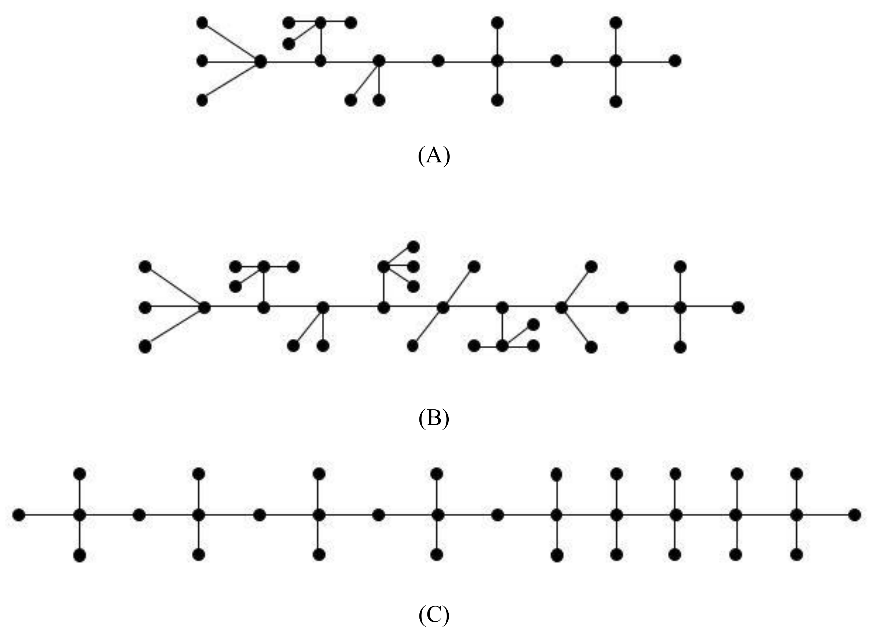
- For , the fourth maximum value isand the equality holds if and only if and such that , and .
- (1.2)
- For , the fifth maximum value isand the equality holds if and only if and such that , and .
- (1.3)
- For , the sixth maximum value isand the equality holds if and only if , such that and .
- (2)
- Suppose that .
- (2.1)
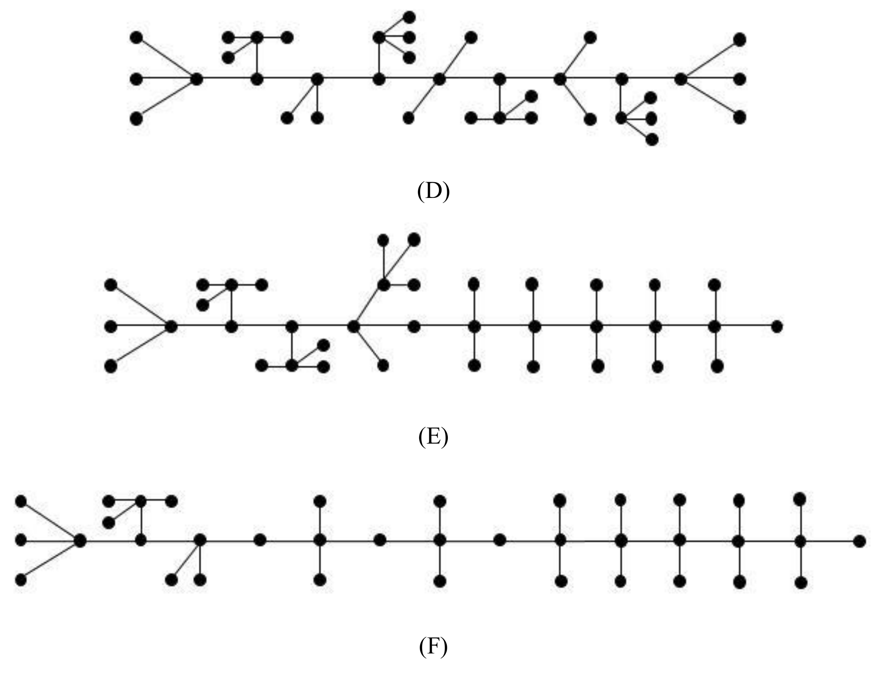
- For , the fourth maximum value isand the equality holds if and only if and such that and .
- (2.2)
- For , the fifth maximum value isand the equality holds if and only if , such that , , and .
- (2.3)
- For , the sixth maximum value isand the equality holds if and only if and such that , , and .
- (3)
- Suppose that .
- (3.1)
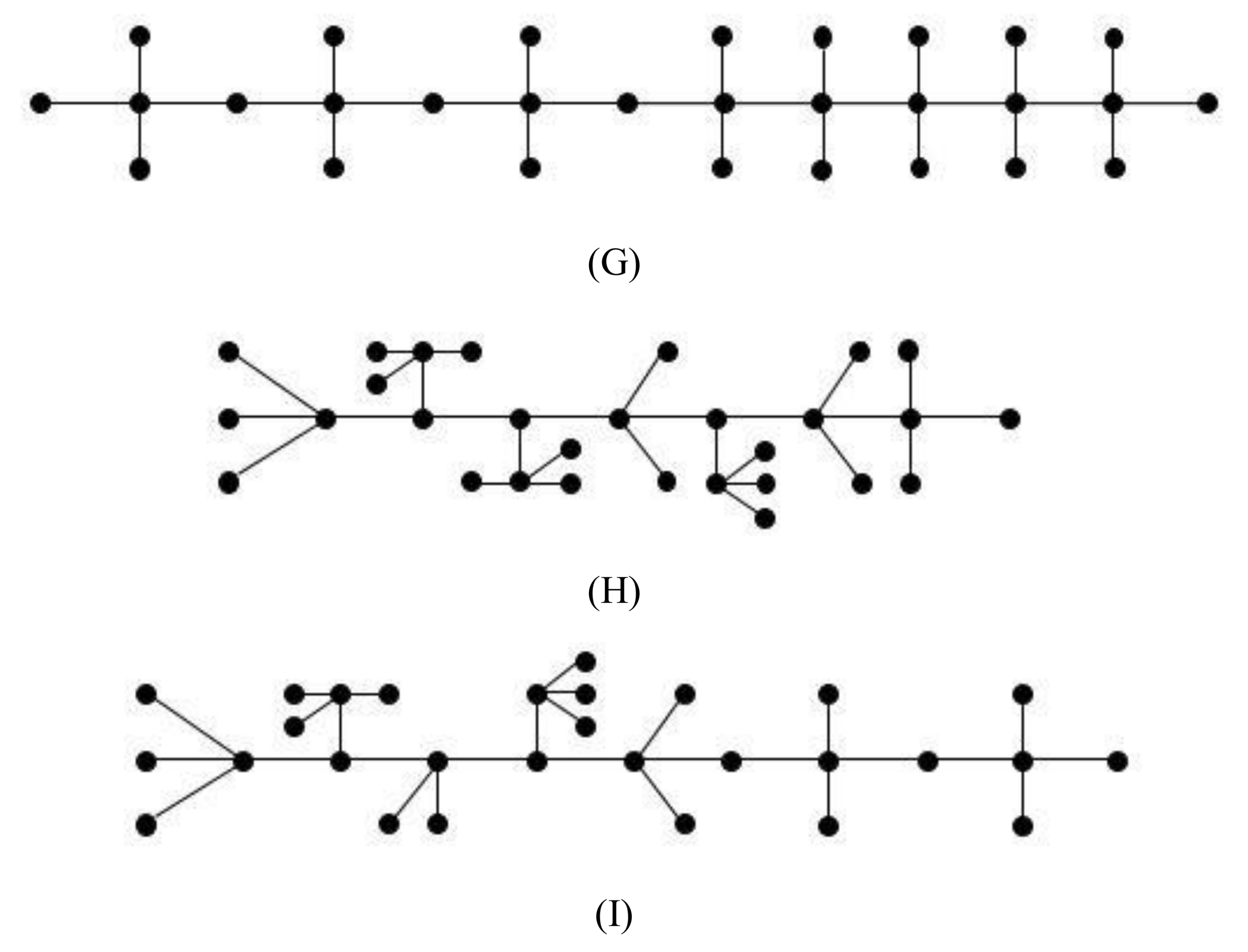
- For , the fourth maximum value isand the equality holds if and only if and such that and .
- (3.2)
- For , the fifth maximum value isand the equality holds if and only if and such that , and .
- (3.3)
- For , the sixth maximum value isand the equality holds if and only if and such that , and .
Proof.
First, we claim that when or . More precisely, from Equation (12),
- when ,
- when ,
- when ,
- when ,
So we may assume that , and or 1. It follows from Equations (5) and (6) that
and
Case 1..
Observe that , , and thus from Equation (13).
If , then by the Equation (12),
If , then by Equation (12),
Case 2..
From Equations (13) and (14), it follows that
and
Now, we consider the two cases: and .
Subcase 2.1..
Clearly, . The proofs will be partitioned into several parts according to the value of : , , .
Firstly suppose that , then, from Equation (14). Note that the case is known to belong to one of the first three minimum values, see Theorem 1-(1.3). If , then from Equation (8), from Equation (17), and by Equation (12),
Next, suppose that , then from Equation (14). If , then from Equation (8), from Equation (17), and by Equation (12),
Subcase 2.2..
In this case, from Equation (18). This time, we partition the proofs according to the value of : , , , , , .
Firstly suppose that , that is, from Equation (17). Note that the cases were known to belong to the first three minimum value, see Theorem 1. If , then from Equation (8), , and by Equation (12),
If , then , and by Equation (12),
Next, suppose that , that is, from Equation (17). Note that the cases were known to belong to the first three minimum values, see Theorem 1. If , then from Equation (8), , and by Equation (12),
If , then , and by Equation (12),
Now, suppose that , that is, from Equation (17). The case was known to belong to one of the first three minimum values, see Theorem 1-(2.2). If , then from Equation (8), , and by Equation (12),
If , then , and by Equation (12),
If , then , and by Equation (12),
If , then , and by Equation (12),
In conclusion, we obtain the following
- (i)
- If , then the fourth, fifth and sixth minimum values are 0.0580155, 0.0736795 and 0.0802936, respectively.
- (ii)
- If , then the fourth, fifth and sixth minimum values are 0.0714748, 0.0737492 and 0.0780889, respectively.
- (iii)
- If , then the fourth, fifth and sixth minimum values are 0.0602202, 0.0715445 and 0.07588419, respectively.
Now, the Equation (11) implies the fourth, fifth and sixth maximum . □
4. Upper Bound for Index of Molecular Trees
In this section, we consider the class of molecular tress and investigated the sharp bound on for this class of graphs.
Let be the set of molecular trees satisfying
and
Theorem 3
([19]). Let T be a molecular tree with n vertices, of which are pendant vertices. Then
with equality holds if and only if .
Obviously, from Equation (1) we obtain
Now let be the set of molecular trees satisfying
and
Theorem 4.
Let T be a molecular tree of order n and pendant vertices, then
with equality holds if and only if .
Proof.
Since T is a molecular tree, we have Equations (2)–(7). Suppose that
that is,
we have
implying that
Thus we have
Substituting them back into Equation (19), we have
with negative coefficients , , , , and . Thus
and equality in above holds if and only if = = = = = = 0, or equivalently, , , , i.e., . □
5. Conclusions
In this paper, we considered more maximum values of the difference , where and R are the atom-bond connectivity index and Randić index, respectively. In particular, we characterized the fourth, the fifth and the sixth maximum chemical trees with respect to the invariant , and thus extended the result by Ali and Du [24] in 2017. It is very challenging to find more maximum values of invariant unless new efficient method is introduced. By using the technique from [19], we also obtained a sharp upper bound for the index of molecular (or chemical) trees with fixed number of pendant vertices. The work on bounds for the index of general graphs and trees is widely open and one can consider many directions.
Author Contributions
Conceptualization, R.H. and Z.D.; methodology, W.N.N.N.W.Z.; validation, R.H., Z.D. and M.K.J.; formal analysis, W.N.N.N.W.Z.; investigation, W.N.N.N.W.Z., R.H. and Z.D.; resources, R.H.; writing—original draft preparation, R.H.; writing—review and editing, R.H., Z.D. and M.K.J.; supervision, R.H. and Z.D.; project administration, R.H.; funding acquisition, R.H. All authors have read and agreed to the published version of the manuscript
Funding
This research received no external funding.
Acknowledgments
This research is supported by the Research Intensified Grant Scheme (RIGS), Phase 1/2019, Universiti Malaysia Terengganu, Malaysia with Grant Vot. 55192/6. The authors would like to thanks the referees for the constructive and valuable comments that improved the paper.
Conflicts of Interest
The authors declare no conflict of interest.
References
- West, D.B. Introduction to Graph Theory, 2nd ed.; Prentice Hall, Inc.: Upper Saddle River, NJ, USA, 2001. [Google Scholar]
- Devillers, J.; Balaban, A.T. (Eds.) Topological Indices and Related Descriptors in QSAR and QSPR; Gordon and Breach: Amsterdam, The Netherlands, 1999. [Google Scholar]
- Todeschini, R.; Consonni, V. Handbook of Molecular Descriptors; Wiley-VCH: Weinheim, Germany, 2000. [Google Scholar]
- Randić, M. On characterization of molecular branching. J. Am. Chem. Soc. 1975, 97, 6609–6615. [Google Scholar] [CrossRef]
- Gutman, I.; Furtula, B. Recent results in the theory of Randić index. In Mathematical Chemistry Monograph. 6; University of Kragujevac: Kragujevac, Serbia, 2008. [Google Scholar]
- Li, X.; Gutman, I. Mathematical aspects of Randić-type molecular structure descriptors. In Mathematical Chemistry Monograph. 1; University of Kragujevac: Kragujevac, Serbia, 2006. [Google Scholar]
- Li, X.; Shi, Y. A survey on the Randić index. MATCH Commun. Math. Comput. Chem. 2008, 59, 127–156. [Google Scholar]
- Randić, M. On the history of the Randić index and emerging hostility towards chemical graph theory. MATCH Commun. Math. Comput. Chem. 2008, 59, 5–124. [Google Scholar]
- Husin, N.M.; Hasni, R.; Du, Z.; Ali, A. More results on extremum Randić indices of (molecular) trees. Filomat 2018, 32, 3581–3590. [Google Scholar] [CrossRef]
- Li, J.; Balachandran, S.; Ayyaswamy, S.K.; Venkatakrishnan, Y.B. The Randić indices of trees, unicyclic graphs and bicyclic graphs. Ars Combin. 2016, 127, 409–419. [Google Scholar]
- Estrada, E.; Torres, L.; Rodríguez, L.; Gutman, I. An atom-bond connectivity index: Modelling the enthalpy of formation of alkanes. Indian J. Chem. Sect. A 1998, 37, 849–855. [Google Scholar]
- Estrada, E. Atom-bond connectivity and energetic of branched alkanes. Chem. Phys. Lett. 2008, 463, 422–425. [Google Scholar] [CrossRef]
- Gutman, I.; Furtula, B.; Ahmadi, M.B.; Hosseini, S.A.; Nowbandegani, P.S.; Zarrinderakht, M. The ABC index conundrum. Filomat 2013, 27, 1075–1083. [Google Scholar] [CrossRef] [Green Version]
- Cui, Q.; Qian, Q.; Zhong, L. The maximum atom-bond connectivity index for graphs with edge-connectivity one. Discrete Appl. Math. 2017, 220, 170–173. [Google Scholar] [CrossRef]
- Dimitrov, D. On the structural properties of trees with minimal atom-bond connectivity index III: Bounds on B1- and B2-branches. Discrete Appl. Math. 2016, 204, 90–116. [Google Scholar] [CrossRef]
- Gao, Y.; Shao, Y. The smallest ABC index of trees with n pendant vertices. MATCH Commun. Math. Comput. Chem. 2016, 76, 141–158. [Google Scholar]
- Shao, Z.; Wu, P.; Gao, Y.; Gutman, I.; Zhang, Z. On the maximum ABC index of graphs without pendent vertices. Discrete Appl. Math. 2017, 315, 298–312. [Google Scholar] [CrossRef]
- Xing, R.; Zhou, B.; Dong, F. On the atom-bond connectivity index of connected graphs. Discrete Appl. Math. 2011, 159, 1617–1630. [Google Scholar] [CrossRef]
- Xing, R.; Zhou, B.; Du, Z. Further results on atom-bond connectivity index of trees. Discrete Appl. Math. 2010, 158, 1536–1545. [Google Scholar] [CrossRef]
- Das, K.C.; Das, S.; Zhou, B. Sum-connectivity index. Front. Math. China 2016, 11, 47–54. [Google Scholar] [CrossRef]
- Das, K.C.; Trinajstić, N. Comparison between the first geometric-arithmetic index and atom-bond connectivity index. Chem. Phys. Lett. 2010, 497, 149–151. [Google Scholar] [CrossRef]
- Raza, Z.; Bhatti, A.A.; Ali, A. More comparison between the first geometric-arithmetic index and atom-bond connectivity index. Miskolc Math. Notes 2016, 17, 561–570. [Google Scholar] [CrossRef] [Green Version]
- Zhong, L.; Cui, Q. On a relation between the atom-bond connectivity and the first geometric-arithmetic indices. Discrete Appl. Maths 2015, 185, 249–253. [Google Scholar] [CrossRef]
- Ali, A.; Du, Z. On the difference between atom-bond connectivity index and Randić index of binary and chemical trees. Int. J. Quantum Chem. 2017, 117, e25446. [Google Scholar] [CrossRef]
- Riaz, A.; Ellahi, R.; Bhatti, M.M.; Marin, M. Study of heat and mass transfer in the Erying-Powell model of fluid propagating peristaltically through a rectangular compliant channel. Heat Transfer Res. 2019, 50, 1539–1560. [Google Scholar] [CrossRef]
- Gutman, I.; Miljkovic, O.; Caporossi, G.; Hansen, P. Alkanes with small and large Randić connectivity indices. Chem. Phys. Lett. 1999, 306, 366–372. [Google Scholar] [CrossRef]
Figure 1.
Chemical trees with the fourth (A), the fifth (B) and the sixth (C) maximum values in Theorem 2-(1).
Figure 1.
Chemical trees with the fourth (A), the fifth (B) and the sixth (C) maximum values in Theorem 2-(1).

Figure 2.
Chemical trees with the fourth (D), the fifth (E) and the sixth (F) maximum values in Theorem 2-(2).
Figure 2.
Chemical trees with the fourth (D), the fifth (E) and the sixth (F) maximum values in Theorem 2-(2).

Figure 3.
Chemical trees with the fourth (G), the fifth (H) and the sixth (I) maximum values in Theorem 2-(3).
Figure 3.
Chemical trees with the fourth (G), the fifth (H) and the sixth (I) maximum values in Theorem 2-(3).

© 2020 by the authors. Licensee MDPI, Basel, Switzerland. This article is an open access article distributed under the terms and conditions of the Creative Commons Attribution (CC BY) license (http://creativecommons.org/licenses/by/4.0/).
Share and Cite
MDPI and ACS Style
Zuki, W.N.N.N.W.; Du, Z.; Kamran Jamil, M.; Hasni, R. Extremal Trees with Respect to the Difference between Atom-Bond Connectivity Index and Randić Index. Symmetry 2020, 12, 1591. https://doi.org/10.3390/sym12101591
AMA Style
Zuki WNNNW, Du Z, Kamran Jamil M, Hasni R. Extremal Trees with Respect to the Difference between Atom-Bond Connectivity Index and Randić Index. Symmetry. 2020; 12(10):1591. https://doi.org/10.3390/sym12101591
Chicago/Turabian StyleZuki, Wan Nor Nabila Nadia Wan, Zhibin Du, Muhammad Kamran Jamil, and Roslan Hasni. 2020. "Extremal Trees with Respect to the Difference between Atom-Bond Connectivity Index and Randić Index" Symmetry 12, no. 10: 1591. https://doi.org/10.3390/sym12101591
Note that from the first issue of 2016, this journal uses article numbers instead of page numbers. See further details here.