Contemporary Snow Changes in the Karakoram Region Attributed to Improved MODIS Data between 2003 and 2018


International Centre for Integrated Mountain Development (ICIMOD), Kathmandu G.P.O. Box 3226, Nepal
*
Authors to whom correspondence should be addressed.
Water 2020, 12(10), 2681; https://doi.org/10.3390/w12102681
Submission received: 20 August 2020
/
Revised: 11 September 2020
/
Accepted: 13 September 2020
/
Published: 25 September 2020
(This article belongs to the Special Issue River Flow in Cold Climate Environments)
Abstract
:Snowmelt significantly contributes to meltwater in most parts of High Mountain Asia. The Karakoram region is one of these densely glacierized and snow-covered regions. Several studies have reported that glaciers in the Karakoram region remained stable or experience slight mass loss. This trend has called for further investigation to understand changes in other components of the cryosphere. This study estimates the comparative snow cover area (SCA) and snowline altitude (SLA) changes between 2003 and 2018 in the Karakoram region and its subbasins, including Hunza, Shigar, and Shyok. We used three different 8-day composite snow products of the Moderate Resolution Imaging Spectroradiometer (MODIS) in this study including (1) Original Aqua (MYD10A2), (2) Original Terra (MOD10A2), and (3) Improved Terra-Aqua (MOYDGL06*) snow products from 2003 to 2018. We used Mann–Kendall and Sen Slope methods to assess trends in the SCA and SLA. Our results show that the original snow products are significantly biased when investigating seasonal and annual trends. However, discarding a cloud cover of >20% in the original products improves the results and makes them more comparable to our improved snow product. The original products (without cloud removal) overestimate the SCA during summer and underestimate the SCA during winter and year-round throughout the Karakoram region. The bias in the mean annual SCA between improved and Aqua and Terra cloud threshold products for the Karakoram region is found to be −1.67% and 1.1%, respectively. The improved (MOYDGL06*) product reveals a statistically insignificant decreasing trend of the SCA on the annual scale between 2003 and 2018 in the Karakoram region and all three subbasins. The annual trends decreased at −0.13%, −0.1%, −0.08%, and −0.05% in the Karakoram, Hunza, Shigar, and Shyok, respectively. The monthly trends were slightly positive overall in December. The annual maximum SLA shows a statistically significant upward trend of 13 m above sea level (m a.s.l.) per year for the entire Karakoram region. This finding suggests a significant uncertainty in water resource planning based on the original snow data, and this study recommends the use of the improved snow product for a better understanding.
1. Introduction
The cryosphere is an important water resource in High Mountain Asia (HMA), and the region is often recognized as the water tower or the third pole because HMA constitutes the largest volume of ice outside the polar region [1]. Understanding snow dynamics is of paramount importance for one-fourth (approximately two billion people) of the global population, who are dependent on meltwater originating from the mountains [2]. Realizing this importance, the Global Climate Observation System (GCOS) recognizes snow as one of the essential climate variables (ECVs). Most studies have focused on glacier change assessments, although the majority of meltwater in most of HMA catchments is from snowmelt [3,4]. Thus, there is still a need for continuous and long-term studies of the snow dynamics of HMA.
Spatiotemporal variations in snow properties are highly heterogeneous in mountainous regions [5]. Historically, snow was manually observed using snow course measurements, which are laborious, expensive and unsafe. Even if available, a snow course measurement represents a single point and may not be representative of an entire area or region [6]. Recent advancements in technology have made it possible for automatic snow sensors, such as snow pillow, gamma-ray and ultrasound sensors, although these methods do not address the spatial snow variability in HMA caused by complex topography and limited observations. Furthermore, continuous field measurements are challenging to obtain in high mountains due to complex terrain and extreme climates [7,8,9]. Because of the vastness of the snow cover area (SCA), it is not possible to carry out field measurements throughout the region. However, remote sensing has significant limitations in terms of precisely estimating the snow water equivalent (SWE). Nonetheless, remote sensing data are widely used for mapping and monitoring the snow cover extent across the globe.
Moderate Resolution Imaging Spectroradiometer (MODIS) snow cover data [10] have been instrumental in understanding the spatiotemporal variability across the globe. The cloud cover and misclassification of snow in MODIS data, due to its wide swath and low spatial resolution, limit its wider application in glaciohydrological studies. Snow and cloud confusion may lead to the overestimation of snow in the daily MODIS product, which further propagates into the MODIS 8-day products [11]. The large sensor zenith angle (SZA) and off-nadir view acquisition cause an overestimation of the snow [12]. The overestimation of snow in MODIS data can be minimized by applying different algorithms [11,12,13,14]. Implementation of improved techniques to derive a snow cover product from MODIS can significantly improve the data quality and minimize the signal-to-noise ratio [15]. Muhammad and Thapa [12] developed an improved MODIS 8-day snow cover product and combined it with the Randolph Glacier Inventory version 6.0 (RGI6.0) [16] for HMA, resulting in new snow cover data with reduced uncertainty. The product is named MOYDGL06* and is freely available for download from the Pangaea repository [17]. The product is approximately 99.98% cloud-free with 3.66% of snow underestimation and 46% overestimation.
Numerous studies observed the snow cover area and snowline altitude in the Karakoram region and upper Indus Basin (UIB) [3,18,19,20]. Immerzeel et al. [3] observed a statistically significant decreasing SCA trend in UIB. On the contrary, Tahir et al. [18] found an increasing trend in snow cover in the Hunza Basin between 2000 and 2009. The annual and seasonal SCA insignificantly decreased in the Gilgit Basin [21]. In addition, Bibi et al. [20] revelated a shift in the snow accumulation and depletion pattern in the eastern Karakoram (Shyok Basin). The postablation season equilibrium line altitude (ELA) remained between 4917 and 5336 metres above sea level (m a.s.l.) from 2000 to 2016 [22]. Likewise, Immerzeel et al. [3] observed the snowline altitude at 2336 m a.s.l. in winter and 4109 m a.s.l. in summer. Khan et al. [23] found the value of the ELA between 4800 to 5550 m a.s.l. in the subbasins of the UIB.
MODIS snow cover products have also been used widely for simulating snowmelt runoff and validating modeled snow properties [3,7,24,25]. Findings of the SCA and SLA from the previous studies in the Karakoram region are significantly inconsistent mainly because of different cloud cover thresholds and cloud filtering approaches. Hence, a comprehensive estimate of snow cover and snowline dynamics is necessary for a better understanding of the cryospheric changes. This study examines the up-to-date SCA and SLA dynamics in the Karakoram region using the MODIS snow product MOYDGL06* [17] and compared the results with the original M*D10A2 products [26] to highlight the limitation of the original products. The improved cloud-free MODIS 8-day snow product for the 2003 to 2018 period is used for SCA and SLA estimations to understand the change in the snow extent and snowline altitude. A digital elevation model (DEM) is used to identify the snowline altitude from the improved MODIS product using the World Meteorological Organization (WMO) recommended approach as implemented by [14]. We explored the potential of using the snowline as a proxy for the ELA which is an important indicator for understanding the mass balance of glaciers. We also investigated the potential of the improved product for studying snow climatology and its applications for glaciohydrological modeling.
2. Study Area
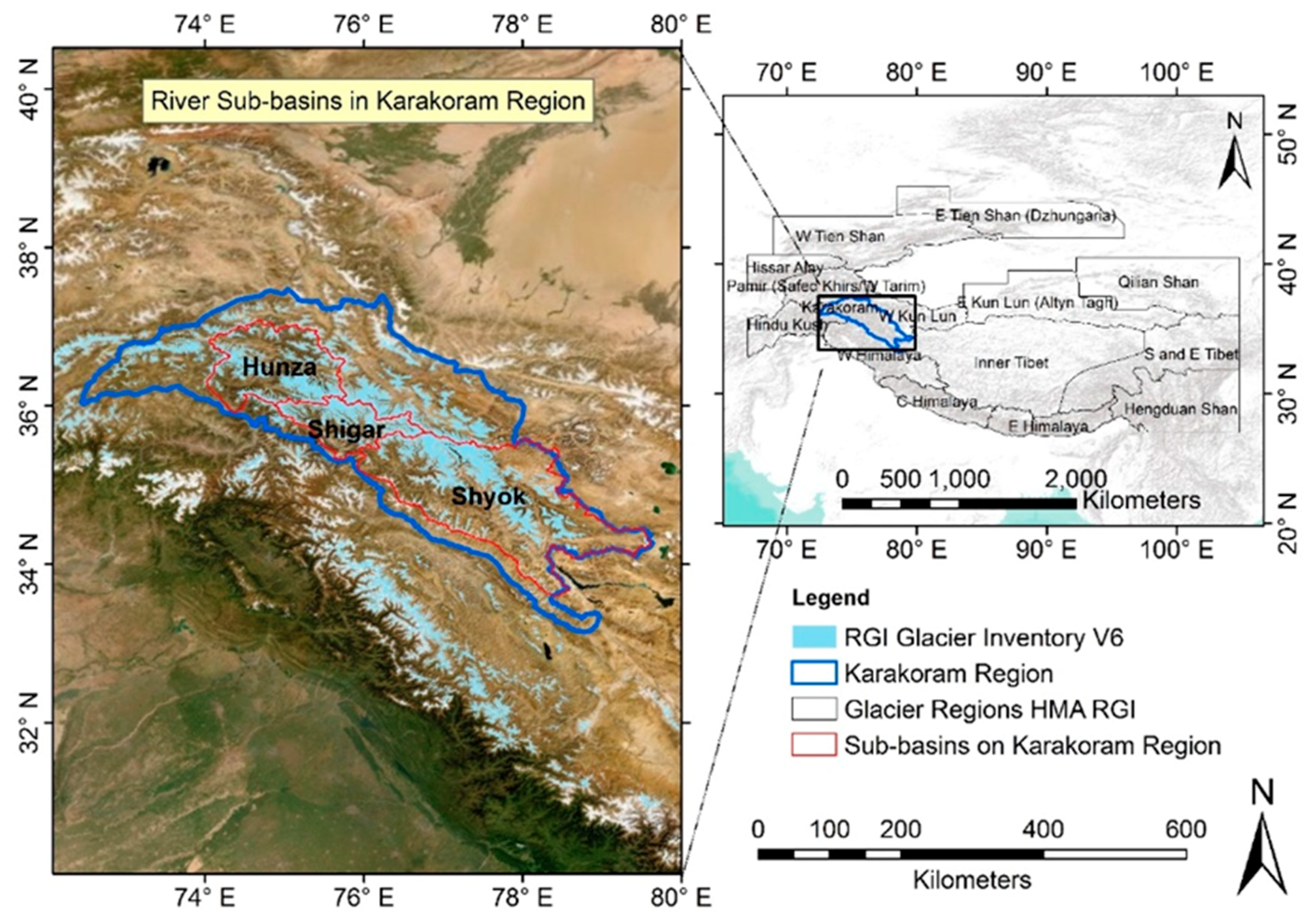
The Karakoram region extends between the longitudes 72.44° to 79.64° E and latitudes 33.14° to 37.47° N, as shown in Figure 1, with an area of 104,010 km2 (Table 1). The altitude of the region ranges from 1236 to 8611 m above sea level (m a.s.l.) with a mean altitude of 4709 m a.s.l. Westerlies are the dominant climatic system in the region. The Hunza, Shigar and Shyok are high-altitude basins of the upper Indus Basin (UIB). More than 60% of the glaciers of the Indus basin are found in the Karakoram region [27] and are mostly fed by avalanches, redistribution by wind, and seasonal snow. Approximately 22% of the Karakoram region is covered by glaciers, of which 27.8%, 24.9%, and 39.03% are found in the Hunza, Shigar and Shyok basins, respectively. The Hunza River Basin is a northern subcatchment of the UIB located in the western Karakoram region of Pakistan. The Hunza river is one of the major tributaries of the Indus River irrigation system, and it contributes approximately 12% of the upper Indus flow upstream of Tarbela Dam [7]. It has a catchment area of 13,745 km2 with an elevation range of 1450 to 7404 m a.s.l. The SCA reaches up to 80% in winter and reduces to 30% in summer [18]. The Shigar Basin is located in central Karakoram. This catchment occupies an area of 7050 km2. The total glacierized area of the catchment is 5701 km2. Some of the well-known and important glaciers in the catchment are the Biafo and Baltoro. The SCA reaches 88% in January and decreases to 10% in August [28]. The Shigar Basin receives approximately 67% of its annual precipitation in winter [29,30,31,32]. The Shyok Basin has a catchment area of 33,419 km2 and is located in the eastern Karakoram. Snow remains a dominant cryospheric component in the basin [33]. The seasonal variation in the SCA over the Shyok River Basin ranges from 27% to 59% with the maximum in February and minimum in July [24].
3. Data
3.1. MODIS 8-Day Maximum Snow Cover Product
Standard 8-day maximum snow cover products from MODIS Terra (MOD10A2, V006) and Aqua (MYD10A2, V006) with a spatial resolution of 500 m were used to extract the SCA and SLA. These data sets were downloaded from the National Snow and Ice Data Center Distributed Data Archive (https://nsidc.org/) for the period between 2003 and 2018. The MODIS snow data is available for the period from 18 December 1999 and 4 May 2002 from through Terra and Aqua satellites, respectively. A comprehensive description of the MODIS 8-day snow products version 6 is available at The National Snow and Ice Data Center (NSIDC) [26].
3.2. Improved MODIS 8-Day Maximum Snow Cover Product
The MOD10A2 and MYD10A2 products were processed to remove clouds and reduced the average snow underestimation of 3.66% and merged to reduce the overestimation of 46% in the improved 8-day maximum snow cover product MOYDGL06* [12]. All these products were used in this paper to analyze snow cover trends and estimate snowline dynamics. The improved cloud-free snow cover product is freely available from the Pangaea repository [17]. The detailed snow data improvement methodology and dataset are described in [12].
3.3. Elevation Data
The snowline elevation from the MODIS product was estimated using the United States Geological Survey (USGS) HydroSHEDS. This dataset is available at https://hydrosheds.cr.usgs.gov. The HydroSHEDS elevation data are hydrologically conditioned data derived from the elevation of the Shuttle Radar Topography Mission (SRTM) at a 3 arc-second spatial resolution. A sequence of the automatic algorithm has been applied to SRTM data, including void filling and filtering, sink identification, stream burning and upscaling techniques.
4. Methods
4.1. Snow Cover Area Calculation
The snow cover area was estimated using original and improved MODIS snow products. The original products were also used with the <20% clouds threshold (as commonly used by previous studies [18,21]) for comparison with the improved product. In the products with 20% cloud thresholds, the original Aqua and Terra images with a percentage cloud cover more than 20% were discarded for the comparative assessment among five different products. The snow cover area was calculated using the total land area instead of the total cloud free pixels to highlight the difference in snow cover area estimation from different products.
4.2. Snowline Altitude Estimation
The SLA can be defined as the elevation above which snow exists after the melt season. However, at the end of the melt season, snow is often patchy in mountainous catchments due to wind erosion, avalanches and other topographic factors. Therefore, it is challenging to represent a snowline at a specific altitude. To overcome this difficulty, the WMO [34] recommended using an elevation band rather than an elevation line, which represents a zone of approximately 50% snow coverage. In this study, the snowline altitude was defined as the elevation band above which there are negligible snow-free pixels.
The snowline altitude was derived from the MODIS snow product and elevation data using the regional snowline elevation (RSLE) method developed by [14]. The snowline has been widely derived using the MODIS snow product in different parts of the world [35,36,37]. Comparisons of MODIS-derived snowlines from high-resolution DEMs and field-based studies have shown good agreement [5,38]. Additionally, the RSLE method by [14] has been widely used to investigate snow dynamics [37,39,40,41,42]. This method estimates the elevation at which the number of snow-free pixels above the elevation line and the number of snowy pixels below the elevation line are at their minimum above and below the elevation line. The snowline altitude was identified by iterating elevation bands from the lowest to highest altitudes in the basin, evaluating the number of snow-covered pixels below and snow-free pixels above the elevation bands. We used elevation data from the USGS HydroSHEDS DEM with a spatial resolution of 90 m. This spatial resolution fulfils the requirement of this study because the MODIS snow product resolution is 500 m. Both products were masked by the area of interest. For each area of interest, the elevation raster was divided into different elevation bins with 10 m intervals, and the corresponding snow-covered pixels below the elevation band and snow-free pixels above the elevation band were evaluated. Finally, the 8-day snowline altitude was selected at which there was lowest snow-covered pixels below and lowest snow-free pixels above the elevation. Detailed information about the snowline algorithm can be obtained from [14].
4.3. Snow Cover and Snowline Trend Analysis
A set of nonparametric tests, i.e., Sen’s Slope and the Mann–Kendall (MK) test, were used to evaluate the trends. A nonparametric test is commonly used for trend analysis in climate research [43]. Sen’s Slope was used to detect the magnitude and direction while the MK test was used to test the statistical significance of the trend. The Sen’s Slope method uses a linear model to estimate the trend slope, and the variance in the residuals should be constant in time, as calculated in [44]:
where xj and xk are the data values at times j and k (j > k), respectively. In general, Sen’s Slope is defined as the median of all linear slopes between xj and xk.
The MK test was originally proposed by [45] and rephrased by [46]. The approach is widely used to test the null hypothesis (H0) of no trend. Each value in a time series is compared with subsequent data values, and depending on whether the data value is higher or lower, the MK test statistic “S” is increased by 1 or decreased by 1. The statistic S can be computed as follows:
where n is the number of data points, xi and xj are the data values in time series i and j (j > i), respectively, and sgn(xj − xi) is the sign function, which is calculated as follows:
The variance is computed as follows:
where n is the number of data points, m is the number of tied groups, and ti denotes the number of ties of extent i. A tied group is a set of sample data that have the same value. In cases where the sample size n > 10, the standard normal test statistic Zs is used and is calculated using the following equation.
Trends are tested at the α = 0.1 level of significance (90% confidence level). When |Zs| > Z1−α/2, the null hypothesis is rejected, and a significant trend exists in the time series. Z1−α/2 is obtained from the standard normal distribution table. In this study, the null hypothesis of no trend is rejected if |Zs| > 1.64 at the 90% confidence level.
5. Results
We assessed SCA and SLA dynamics over the Karakoram region and its subbasins: Hunza, Shigar, and Shyok using open-source software R (https://cran.r-project.org/) and RStudio (https://rstudio.com/). Ggplot2 package (https://ggplot2.tidyverse.org) was used for data visualization. The SCA and SLA were examined between 2003 and 2018 for two dimensions: (i) interannual variability and (ii) intra-annual variability. A comparative basin-wide assessment was carried out using the original snow cover products, MYD10A2, MOD10A2, original products with <20% cloud cover, and the improved snow product MOYDGL06*.
5.1. Interannual Variability in SCA
The mean annual SCA from 2003 to 2018 in the Karakoram region and subbasins is shown in Figure 2. A comparative analysis of the mean annual SCA between the NSIDC original products, original products with 20% cloud threshold and our improved snow products reveals a significant underestimation in the original product. The results are mainly attributed to a large number of misclassified snow pixels in the original products. The cloud cover statistics are shown as percentages (>5 to >50) against the number of images in the original products in Table S1. The original 8-day Aqua and Terra snow products contain 15% and 9% clouds on average, respectively, in the Karakoram region. The Terra and Aqua 295 and 417 images contain more than 5% clouds on average, respectively. The <20% cloud threshold of the original snow reduces the annual variability to some extent. However, the cloud threshold products are still biased as compared to the improved product as depicted in Figure 2. The bias between improved and Aqua and Terra cloud threshold products for the Karakoram region is found to be −1.67% and 1.1%, respectively. This value is even higher (3.9% and 3.6%) in the original Aqua and Terra product. Therefore, we analyzed the snow dynamics in the improved cloud-free MOYDGL06* product. The average annual SCA of the Karakoram region between 2003 and 2018 is 67,606.5 km2, which is 65% of the total extent. The winter annual SCA fluctuates between 82% and 93%, whereas the summer SCA varies between 32% and 43%. In addition, the SCAs in Hunza and Shigar are 77%, whereas 64% of the Shyok Basin is covered by snow. The interannual SCA varies significantly during the study period. The annual average area covered by snow for Hunza ranges from 74% to 82%, with the lowest and highest snow occurred in 2007 and 2009, respectively. In contrast, Shigar received its maximum annual snow in 2009 (81%) and minimum in 2007 (72%). Shyok experienced its minimum annual snow in 2016 and its maximum in 2015. The detailed annual SCA statistics are presented in Table 2 and Table S2. The time series of annual maximum and minimum SCA are also shown in Figures S1 and S2. The original MODIS snow products underestimate the average annual SCA in the subbasins due to significant cloud cover variability (Figure 2), indicating high spatial variability across the region. The annual snow cover area is negatively biased in the original M*D10A2 snow products. On the contrary, the Aqua threshold product has random under- and overestimation bias compared to the improved product. The Terra threshold product shows modest underestimation throughout the study period. In addition, the difference for the year 2012 is significantly large (>30% less snow cover area in MYD10A2 compared with the improved snow MOYDGL06* in the Shigar Basin). Original and threshold products show a comparable mean annual maximum SCA variability in both Aqua and Terra because of fewer clouds (<20%) during the snow accumulation season.
The MK test was applied to determine the annual SCA trend at a 90% confidence level in the Karakoram region and subbasins. The Sen’s Slope estimator was used to determine the magnitude of the trends. Statistics analysis of the trends is given in Table 3 and Table S3. The annual minimum and mean snow exhibit contrasting trends in the original (MOD10A2 and MYD10A2) and improved products. This difference is reduced in the cloud threshold products except in a few cases with remaining bias. The magnitude of the annual maximum SCA trend using original and threshold products is equal across all spatial domains with a statistically significant negative trend in the Shigar and Shyok subbasins. The improved product shows that the annual minimum SCA is significantly (p = 0.1) decreasing in Shyok and insignificant in the other two basins. The annual average snow cover decreased by −0.13% in the entire Karakoram and −0.1% in the Hunza Basin. Similarly, the annual maximum SCA shows a decreasing trend, except in Shigar, where it is increasing at a rate of 0.22% per year. The most negative maximum snow trend is 0.23% per year in the Shyok Basin.
We compared the annual average snow cover trend for two equally divided temporal windows and the entire study period, 2003–2010, 2011–2018, and 2003–2018, to understand the short-term and overall SCA variability. There are no statistically significant trends in any of the observed temporal windows in the observed period. Overall, the Karakoram region and Shyok Basin exhibit a positive trend in the annual average SCA between 2003–2010 and 2011–2018, whereas the long-term trend from 2003 to 2018 is negative. This result is due to the large interannual fluctuation in the SCA in the respective period. In contrast, the annual average SCA in Shigar indicates a negative trend in all three temporal windows. Similarly, the snow cover decreases during the first half and the overall study period in Hunza, although a slightly positive SCA is shown during 2011–2018. Despite contrasting characteristics in the short-term analysis, a decreasing regional signal was observed in the long-term SCA trend.
5.2. Intra-Annual SCA Variability
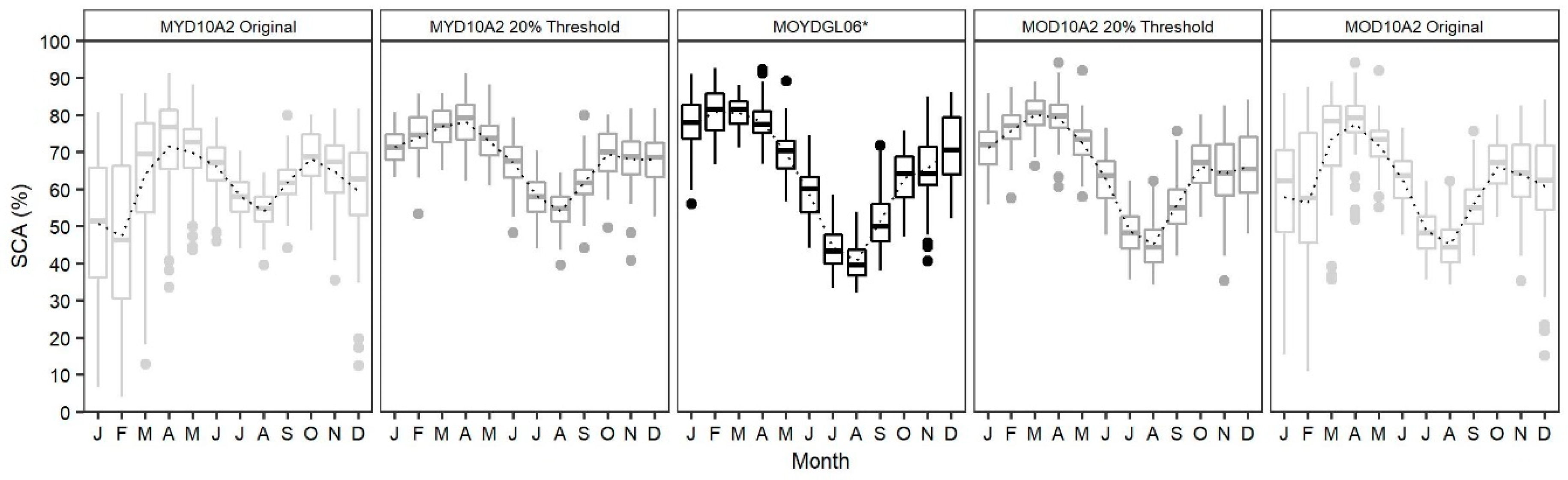
The seasonal variability in the SCA (%) derived from the original M*D10A2, <20% cloud threshold, and improved snow MOYDGL06* products in the Karakoram region is shown in Figure 3. The box and whisker plots represent quartiles of 8-day SCA variability at a monthly scale. The results indicate that the mean SCA is lowest in August in the original Terra (45%), cloud threshold Terra (44%) and improved product (41%) coverage. The lowest snow from Aqua is 48% in February, which is unexpected and attributed to persistent clouds (40%). However, this signal was not observed in the Aqua < 20% cloud threshold product. The mean SCA is the highest by 81% (median SCA = 82%) during late winter and early spring in the improved snow product. In contrast, the highest mean snow cover in the M*D10A2 products are comparatively low with 72% in Aqua and 78% in Terra during midspring. The monthly SCA variation shows conspicuous differences between different products. The maximum median snow cover extent was observed during March (81%) and April (79%) in the Terra and Aqua <20% cloud threshold products, respectively. The original MODIS product produces a bimodal distribution of intra-annual variation in the SCA, whereas the cloud threshold and improved products show a unimodal distribution. Generally, a bimodal distribution is common in the monsoon-dominated catchments and unimodal in the westerly-dominated regions [47]. However, the original product shows a bimodal distribution in the westerly-dominated Karakoram region. The bimodal pattern is attributed to the inherent uncertainty in the M*D10A2 products causing higher SCA variability. However, the cloud threshold products have a similar pattern to the improved data, with a noticeable difference during the winter months. Thus, the 8-day improved snow cover provides accurate snow cover information compared to the 8-day MODIS original and cloud threshold snow cover products.
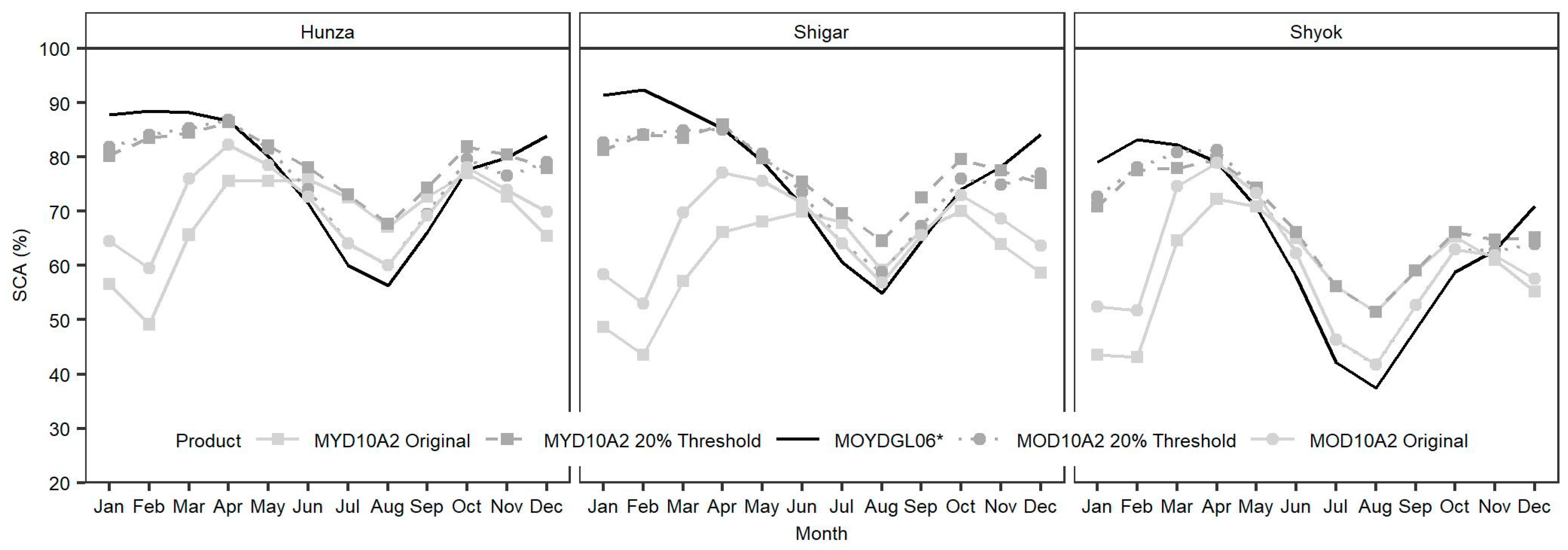
The intra-annual (mean monthly) SCA variability using the original M*D10A2, 20% cloud threshold and MOYDGL06* snow products for individual basins is shown in Figure 4. The individual basins and the entire Karakoram region show a similar pattern on a monthly scale. However, a significant difference is observed in the winter snow between the M*D10A2 and improved MOYDGL06* products (Figure 4). The original M*D10A2 products incorrectly show lower SCAs during winter. However, the improved product shows that the monthly mean SCA reaches its peak in February and is lowest in August. The <20% cloud threshold products indicate a maximum snow extent during April, which is somehow shifted from than the peak season. This may cause a dilemma in assessing the climate change impact using the product. The data-limited maximum snow shift may cause confusion between global climate change and data limitation. Thus, the original and cloud threshold M*D10A2 products are not recommended for snow climatology and hydrology. The analysis of the improved MODIS data shows a smooth increase in the SCA from September to February and a decrease from March to August. The duration from September to February is the snow accumulation period and March to August is the ablation period. For example, Figure 4 shows that 80% of the Shyok Basin was covered by snow between February and March, which reduces to <40% in August.
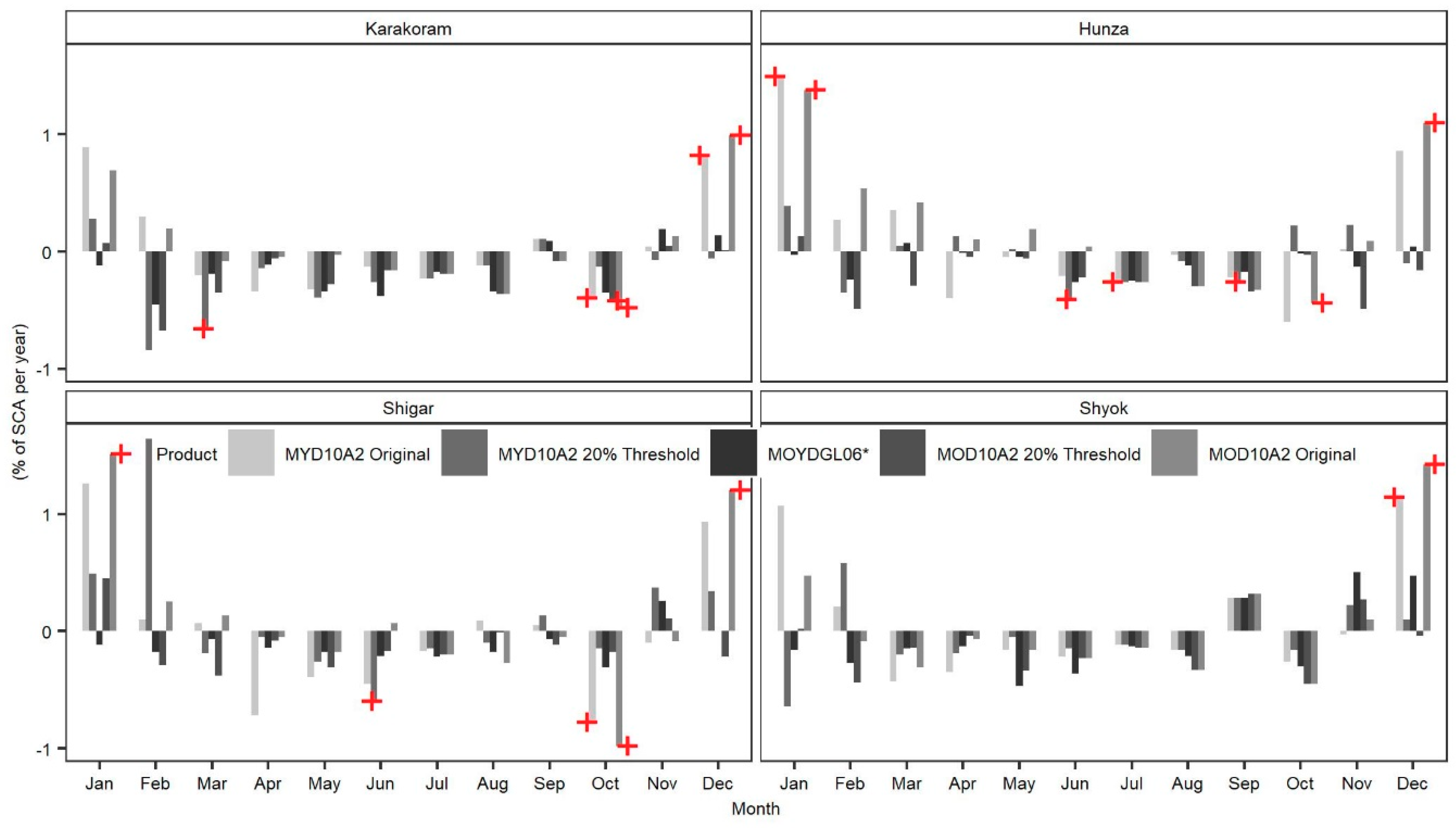
The monthly mean SCA variability is shown in Figures S3–S6 and the trends are presented in Figure 5 and Table S4 for all spatial domains. A distinct overestimation during summer and underestimation during winter were observed across all the regions in the original and cloud threshold products. The comparison of all the five snow products shows a significant difference. The magnitude of the trend ranges from 0.007% to −0.47% per year in the improved product and from −0.84% to 1.64% per year in the cloud threshold products. The trend reaches between −0.98% and 1.51% per year in the original products. This finding indicates a significant reduction and increment in the monthly SCA trend in the original and cloud threshold products. The M*D10A2 and cloud threshold products (except Aqua in the Shyok Basin) show a positive trend throughout January. In contrast, the improved snow (MOYDGL06*) product signifies a negative trend, although all of these trends are statistically insignificant. All products show a similar decreasing tendency for the months from March to August and October in the Karakoram and Shyok. Conversely, September and December show increasing SCA trends in the original Aqua and improved products in the Karakoram and all the products except the Terra cloud threshold in Shyok. In general, the original products display growing SCAs in December and January throughout the study region. Though, the cloud threshold products also exhibit opposite trends during December, which stresses the need for improvement during winter months. The improved product found slightly increased snow cover trends during March and April in Hunza. The SCA in November increased in the Karakoram, Shigar and Shyok, and decreased in Hunza. This analysis shows a heterogeneous snow cover trend within the Karakoram region.
5.3. Interannual Variability in Snowline Altitude
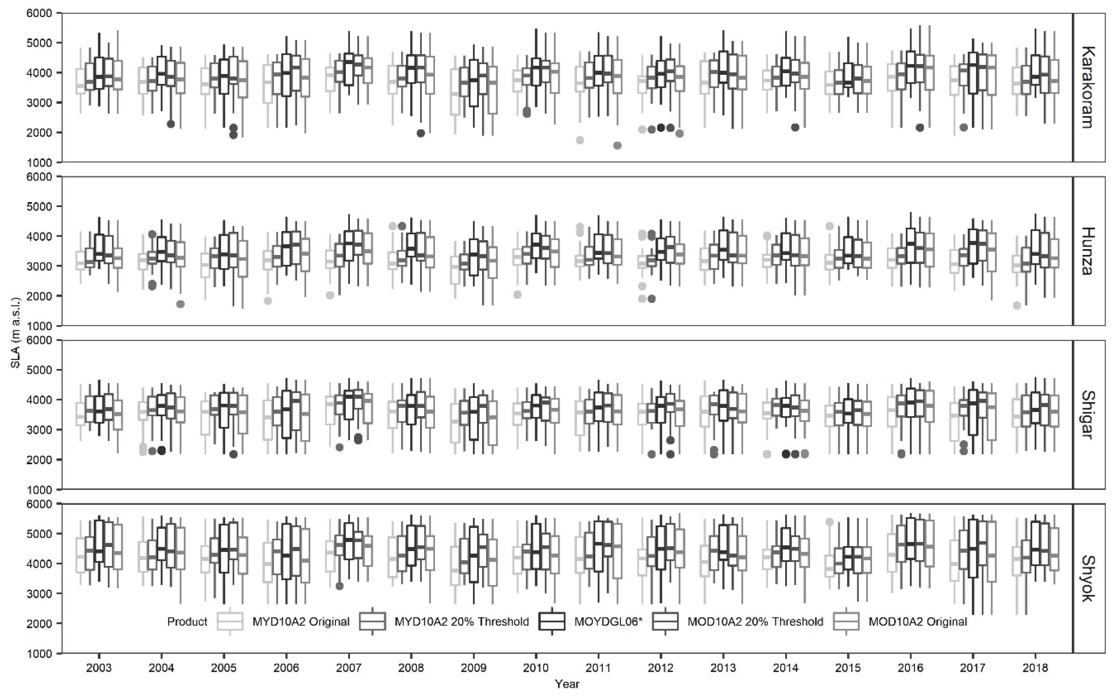
Interannual snowline altitude variability is estimated using all the snow products and HydroSHEDS Elevation data are presented as an annual boxplot in Figure 6. Compared to the original and cloud threshold snow, improved MOYDGL06* product provides enhanced snowline altitude information. The median SLAs throughout the study period (2003–2018) derived from the improved snow product is 4019 ± 736, 3507 ± 594, 3783 ± 696 and 4475 ± 812 m a.s.l. for the Karakoram, Hunza, Shigar, and Shyok, respectively. All of these values are higher than the SLA values derived from the MODIS original snow products. An underestimation was observed in the SLA derived from the Aqua cloud threshold product. On an annual scale, the median SLA from Terra cloud threshold product closely resembles the improved product. The original snow products (M*D10A2) and Aqua cloud threshold product were not successful in representing the annual median SLA dynamics represented by the thick black solid line in Figure 6 due to the underestimation of the SCA. The size of the box whiskers indicates that the first and third quartiles of the original products are lower than the improved product, indicating the underestimation of the SLA. Among all four areas, the 8-day snowline variability in Shyok is the highest of all three products. A regional signal of lower SLA fluctuation was observed in 2015 in all the products. The SLA values in the improved product are highest in Shyok and lowest in Hunza and Shigar. This noticeable difference between Shyok and Hunza–Shigar is due to the steep topography in Hunza–Shigar that enhances snow avalanches from steep snow accumulation areas to the bottom of a hill slope. Approximately 56% of the Hunza and 47% of the area in the Shigar Basin has a slope greater than 25 degrees, which favours snow avalanches and redistribution. In contrast, the SLA of the Shyok Basin in the eastern Karakoram is the highest, where the intensity of the westerlies is weakest (compared with the other two basins).
The annual SLA summary for the Karakoram region and its three basins is shown in Table 4 and Table S5. The annual average SLAs for the Karakoram in MYD10A2, 20% MYD10A2 cloud threshold, MOYDGL06* MOD10A2 and 20% MOD10A2 cloud threshold are 3652, 3807, 3991, 3817 and 3968 m a.s.l., respectively. A similar pattern of underestimation is demonstrated by the mean annual maximum SLAs. Original and cloud threshold products provide nearly equal maximum annual SLAs throughout the study area. The annual minimum SLA shows lower values in the original and cloud products compared to the improved product. This highlights the underestimation of the SLA in all the original products even at the annual scale. The three basins in the Karakoram exhibit analogous behaviour. The annual SLA fluctuates in the improved snow product compared to the original snow products. The annual snowline exhibits immense spatial variability in the Karakoram region, with mean annual maximum values of 4655, 5259, and 5145 m a.s.l. in MYD10A2, MOYDGL06*, and MOD10A2, respectively. The mean maximum annual SLA in the Shyok is the highest among the basins and the lowest SLA occurs in the Hunza. Similar patterns were observed in the mean annual SLA estimates. The snowline elevation shows a gradually decreasing trend from the eastern to western Karakoram. Specifically, the eastern Shyok basin has a higher snowline altitude than the central and western regions.
The results of the annual SLA trend analysis for the Karakoram region and its subbasins between 2003 and 2018 are presented in Table 5 and Table S6. The annual SLA shows a similar pattern in the improved and original Terra products throughout the region, whereas the Aqua estimates an opposite pattern in some cases in the annual minimum and average series. This signal is more prominent in Aqua cloud threshold product. For example, negative trends in the annual minimum SLA were identified using the Aqua products in the Karakoram and Shyok, whereas improved products show a constant and positive trend. Likewise, the original Aqua shows a negative trend in the annual maximum SLA for Hunza and Shigar, whereas the opposite trends are noticed in the Terra and improved products. The annual minimum SLA trend in the Karakoram region is strongest using the improved snow data, with a rate of 14.33 m a.s.l. per year. The annual average SLA in the improved product exhibits an increasing trend with a statistically significant trend of 8.03 m a.s.l. per year in the Karakoram region. The snowline is often taken as a proxy of the ELA and used for understanding the glacier mass balance [22]. The maximum SLAs are extracted using the improved snow product for each year (Figure S7) and used to estimate the trend (Table S6). The increasing trend of the maximum annual SLA during 2003–2018 is observed in all the subbasins. The rate of increase in the annual maximum snowline is highest (13 m a.s.l. per year) and statistically significant at the 90% confidence level on a regional scale and lowest (13 m a.s.l. per year) in the Shigar Basin.
The annual average SLA trends in the three defined temporal windows are estimated similarly to the SCA (Table S7). Our results show that the annual average SLA rises in the Karakoram region during 2003–2010, 2011–2018 and 2003–2018. In contrast, the Hunza Basin experiences a rising SLA from 2003 to 2010 and a falling SLA from 2011 to 2018. Shigar and Shyok show decreasing snowlines during 2003–2010 and 2011–2018, although the overall trend is rising for the entire period from 2003 to 2018. The most striking results are the rising SLAs in Hunza, where the mass balance was stable or slightly negative until the end of the first decade of the twenty-first century [27,48]. Our findings do not support a positive glacier mass balance in the Karakoram region and its subbasins throughout the study period.
5.4. Intra-Annual Variability in Snowline Altitude
The spatiotemporal variations of the SLA are assessed in the Karakoram region and its subbasins. The seasonal variability in the 8-day SLA is presented in Figure 7. The box whiskers represent quartiles of the monthly variability in the snowline estimated during 2003–2018. A clear underestimation of the SLA throughout the study period was observed by the original and the cloud threshold products across all the study sites as indicated by the thick line drawn inside each box in Figure 7. All products show a significant fluctuation in SLA during autumn and winter months. The snowlines are lowest between January and February throughout the region using all products. The lowest monthly median SLA using the improved MOYDGL06* product is 3149, 2957, 2623, and 3385 m a.s.l. in the Karakoram, Hunza, Shigar, and Shyok, respectively. The time of the minimum snowline coincides with the observed maximum SCA. In contrast, the minimum median SLA estimates in the original snow products are dissimilar to the SCA statistics. The highest monthly median SLA was observed in August using all products throughout the region. This observation indicates that the SLA estimates represent the snow dynamics better than the SCA in the original products at the seasonal scale. Original and cloud threshold products provide nearly identical monthly median values indicating the robustness of the snowline algorithm to deal with the cloudy image to some extent. However, we recommend the use of the improved product to understand snow variability more confidently. The median monthly SLA in Shyok using the improved product is the highest (5545 m a.s.l.). For the Karakoram region, the highest monthly median SLA is 4999 m a.s.l. The snowline varies significantly in autumn and winter due to snowfall and seasonal snow onset. The snowline starts to shift downward after August due to the combined effect of a lower temperature and fewer precipitation events and reaches its minimum value in January and February.
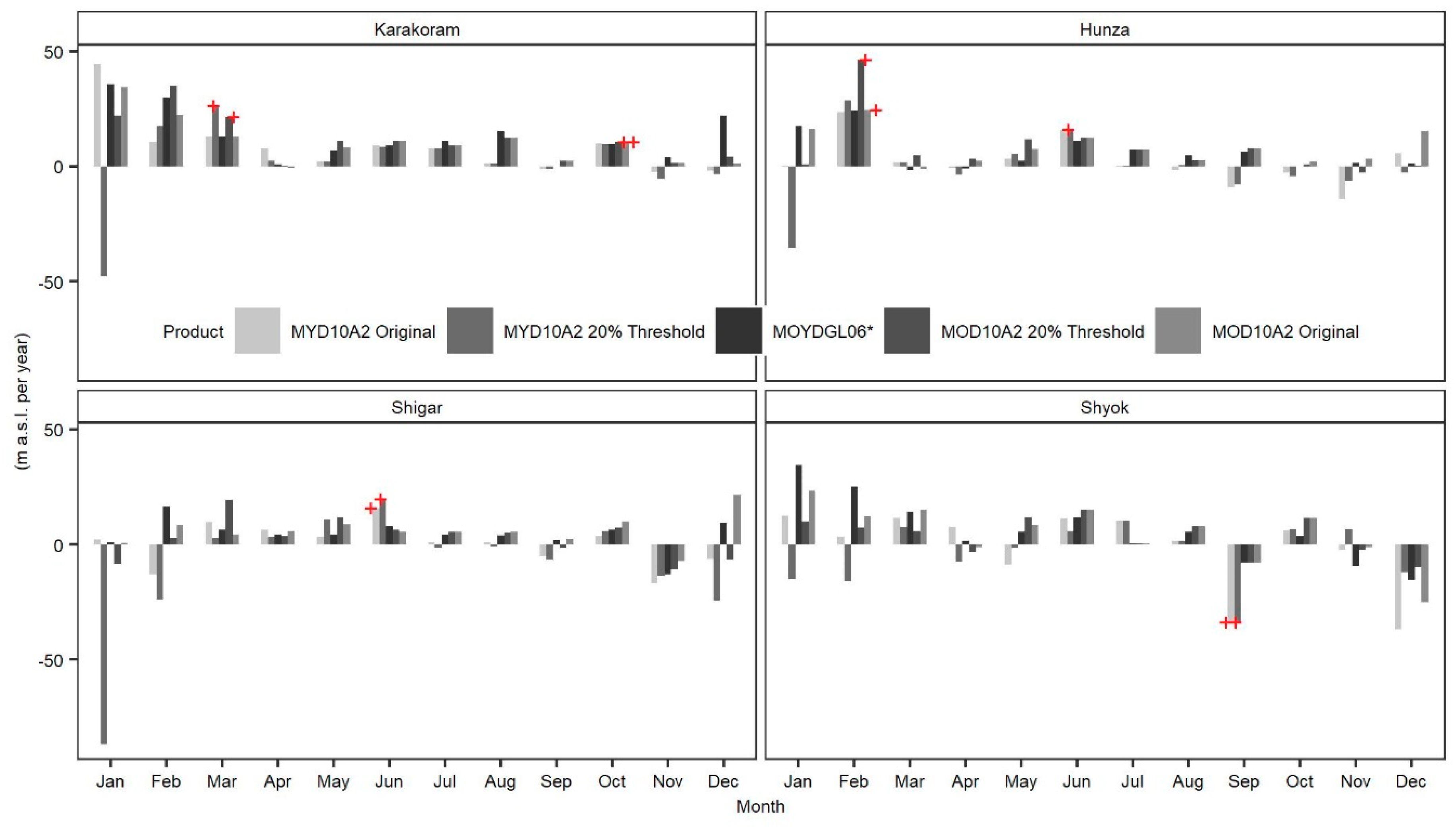
The annual SLA trends suggest that finer temporal resolution data capture the snow dynamics. The monthly trend analysis is presented in Figure 8 and Table S8. A corresponding time series of monthly SLA are plotted in Figures S8–S11. An underestimation of the SLA (lower SLA values) is observed in both original and cloud threshold products. There is a large discrepancy in the trend calculated from the original and cloud threshold products. In particular, the Aqua snow product mostly exhibits a contrasting trend compared with the other products. The improved product shows an increasing tendency in the entire monthly SLA series in the Karakoram region, although the trends are not statistically significant, owing to the relatively short period of analysis. Nonetheless, the trends are stronger in the winter months. Similarly, most of the monthly SLA trends in the individual basin are also negative except March and April for Hunza, November for Shigar and September, November and December for Shyok. The spatial and temporal monthly SLA trend indicates an inconsistent variation.
6. Discussion
We used an improved MODIS snow product (MOYDGL06*) and compared the results with the original M*D10A2, and cloud threshold products to characterize spatiotemporal SCA and SLA variations in the Karakoram region and its major subbasin. Most of the SCA and SLA trends are statistically insignificant in the relatively short observation period which limits the climate-driven physical and statistical explanation of snow dynamics which are often important aspects of climate research. We admit that the derived trend should not be understood as the signal of long term climate trends. However, the analysis of this study does provide the pattern of snow cover area change and highlights the importance of improved products over original and cloud threshold snow products. The annual SCA indicates an insignificant decreasing trend in the Karakoram region and its basins except for Shigar, where the annual maximum SCA increases by 0.22% per year. We also analyzed the monthly mean SCA, indicating a slightly positive trend, especially in the months of November and December throughout the region. However, the trends decrease during spring, particularly in March and April and during summer months. The overall spatiotemporal SCA analysis shows significant heterogeneity in the Karakoram region. In addition, the annual and monthly SLAs show higher snowline altitudes in Shyok compared with Shigar and Hunza. The higher SLA of Shyok is mainly due to weak westerly disturbances compared with the Hunza and Shigar basins. The annual average and maximum SLA of the entire Karakoram region show a statistically significant positive trend in contrast to the monthly insignificant SLA trend.
The quantitative comparison of SCAs in the original products (MYD10A2 and MOD10A2), cloud threshold and improved products (MOYDGL06*) show a large underestimation in the original products on the annual scale (Figure 2). A noticeable difference is observed in the original products with a <20% cloud threshold. This difference is mainly due to the presence of clouds at higher altitudes in the original products. The underestimation is high in the Aqua snow product due to its afternoon revisit time when clouds become dense. In contrast, the seasonal SCA comprises both overestimation and underestimation. The overestimation is mostly found during the summer and early autumn, and the underestimation is found during winter and spring. The summer overestimation is mainly due to the misclassification of clouds as snow at lower altitudes and snow as clouds during winter at higher altitudes. Clouds are a primary constraint in optical remote sensing when estimating snow cover, particularly in mountainous catchments. Additionally, a larger SZA [49] and a wide swath of MODIS cause significant overestimation of snow [50,51]. The presence of clouds in the original products could even alter the trend pattern (e.g., min and mean annual SCA trends, as shown in Table 3). At the monthly scale, the original products show an inverse trend compared with the improved snow product, mostly during winter months.
We compared the annual minimum SCA calculated in this study with the Randolph Glacier Inventory version 6.0 (RGI6.0) glacier boundaries and found that the annual minimum snow cover estimates are higher than the total glacier cover. The snow cover is usually more than the glacier cover, as there are firn and perennial snow at high altitudes. Although the old glacier ice is not necessarily mapped by MODIS, the uncaptured ice is less than the firn and perennial snow at high altitudes. Hasson et al. [52] removed clouds in the snow product and found a decreasing trend in Hunza, Shigar and Shyok’s annual average snow cover analysis. Despite the increasing trend in winter precipitation in the region [18,29], the annual SCA is decreasing according to the results of this study. This finding could be explained by enhanced melting from the observed warming during winter [53,54]. The Khunjerab climate station in Hunza, which is located at 4710 m a.s.l., also shows an increasing trend in both annual and seasonal temperatures [21,55]. On the other hand, earlier studies have shown an increasing trend in the SCA [18,24,33]. The difference could be associated to the method used for removing clouds and the observation period. We used different filters to remove clouds and convert cloudy pixels to snow or not snow, whereas many studies adopted the threshold method (cloud <10%, 20%) to avoid cloudy images. The 20% threshold method provides a similar trend as the improved product in annual SCA series in most cases but the magnitude of the trend differs. The threshold method is susceptible to missing important snow information because the original products have significant uncertainity. Our analysis shows that 122 Terra images and 189 Aqua images (out of 735) have more than 20% clouds persisting on eight consecutive days in the Karakoram region during our study period. The cloudy images are even more abundant in the individual basins (Table S1). A comparison of the annual average SCA and SLA trends between the two different temporal windows shows heterogeneous snow characteristics (Table S7). In the Karakoram region, the annual average SCA shows a slightly increasing trend during 2003–2010 and 2011–2018 in contrast to the SLA upward trend. Similarly, the SCA in Shigar decreases (moving upward) during 2003–2010 and 2011–2018. A possible explanation for this difference in SLA and SCA is the key assumption made in the snowline altitude algorithm. The snowline is a theoretical line above which all areas are considered to be snow-covered and all areas below are snow-free. Actually, this is not always realized on the ground, particularly during the melting season. Thus, the snowline is often explained as a natural surrogate value because it represents an average snow line in a predefined region. However, the Karakoram region exhibited downward SCA and upward SLA trends from 2003 to 2018. Similarly, the SCA in the Shyok Basin exhibits a consistent pattern between the SLA and SCA during 2003–2010 and 2011–2018 with an increase in the SCA when the SLA moves downward and vice versa from 2003 to 2018.
The improved product indicates a slight rise in the annual SLA across the Karakoram region from 2003 to 2018. The mean annual maximum SLA is 5259, 4636, 4637, and 5603 m a.s.l. in the Karakoram, Hunza, Shigar, and Shyok, respectively. These values are close to the range identified by an earlier study [23]. However, our improved MODIS-based mean annual maximum SLA for Hunza is slightly lower than those of [22] (average ELA = 5176 m a.s.l.), estimated from Landsat. The slight difference is due to the spatial resolution and methodology used for snowline estimation. The annual maximum SLA shows a rising pattern over the entire Karakoram region. Huss and Hock [56] also projected an upward trend in the regionally average glacier ELAs between 100 and 500 m during 2010 to 2100 for southwest Asia. The magnitude of the SLA trend is high in Hunza and low in Shigar and Shyok. These findings suggest significant spatial variability in the SLA. In addition, the ELA in Hunza and Shigar are comparatively lower, mainly due to the influence of strong westerly disturbances and steep terrain. Our results agree with earlier studies [22,57], who also identified a strong east–west gradient in precipitation patterns and the ELA in this region. No trend is statistically significant in the individual basin, whereas the Karakoram region shows a significant positive trend. Our snow cover estimates from 2003 to 2018 in the Karakoram region are in line with the recent slight mass loss of glaciers [27,48,58,59]. The short-term estimates during 2003–2010 and 2011–2018 mostly indicate an increase in the SCA. Our areal expansion of snow cover may not necessarily represent glacier mass changes because thickness and surface elevation change is the most reliable estimate of glacier mass balance [60,61]. Although the annual snowline is useful to approximate the ELA and characterize the glacier mass balance, for an improved understanding of the accumulation and melt processes of snow, more field-based observations of the variables, e.g., snow depth and snow water equivalent, should be carried out.
Our analysis shows that the original NSIDC snow cover product (M*D10A2) contains significant uncertainty, which is mainly due to the cloud coverage and overestimation in the original products because of the larger SZA. The twenty percent threshold method also shows some uncertainty at all monthly, seasonal and annual scales. The summer overestimation is due to the larger SZA and the winter underestimation is the result of the misclassification of snow as cloud. The underestimation of snow during winter will result in a reduced snowmelt during the spring season when it is the major discharge source. Similarly, this underestimation may result in undercatching the enhanced snowmelt. Additionally, summer snow overestimation leads to more river runoff and meltwater generation. The improved product reduces these uncertainties and will eventually improve the snowmelt estimation when used in glaciohydrological modeling. The improved product uses spatial and temporal filters to recover the snow pixels from the adjacent before and after images. This criterion may lead to some uncertainty in snowmelt simulations from the improved product, particularly in the peak ablation season. However, the uncertainty in glaciohydrological modeling is expected to be negligible because the snow underestimation (recovered in our improved product) is insignificant on average by 3.66% in the region [12]. In addition, only part of the 3.66% snow recovered in lower altitudes may cause some uncertainty as the high altitude areas are usually snow-covered until the late ablation season. Therefore, we suspect a significant uncertainty in water resource planning based on the original snow data. Although the MOYDGL06* product has significantly improved the snow dynamics in the region, for better understanding, we suggest observing the snow depth, snowmelt, and snow water equivalent. It is important to mention that the SCA does not provide information about the water content in the snowpack. Thus, in addition to SCA and SLA assessments, we also recommend the assessment of the snow water equivalent to investigate the change in the water content of snowpacks and understand the change in water availability in the region. The MOYDGL06* product may be useful to improve the quality of the existing coarser snow water equivalent products by reducing overestimation in the extent and underestimation due to cloud cover.
7. Conclusions
This study assesses the variability in SCA and snowline altitude in the Karakoram region and its major river basins. In comparison to the previous snow studies, we examined the monthly and annual snow cover patterns using the improved MODIS snow product MOYDGL06* in the Karakoram region. Our results show that there is a significant difference in SCA and SLA statistics derived from original, <20% cloud threshold and improved products. The annual SCA in the improved product exhibits an overall decreasing pattern except for the annual minimum SCA series in Shigar, whereas the original product shows mixed trends. However, none of the trends are statistically significant in the improved product except for the annual maximum SCA of 0.22% per year in Shyok. The negative trend of the snow cover area is also verified by the rising pattern of the snowline altitude. Thus, it is found that the simultaneous assessment of the SCA and SLA provides a more robust estimate of the snow cover change. The cloud threshold Terra product successfully captured the annual SCA trend in most cases. The improved product reveals that the highest snow coverage was during February–March and the lowest snow coverage was in August. In contrast, the original and cloud threshold products overestimated the SCA during summer and underestimated the SCA during winter, which may constrain seasonal snow cover changes and associated glaciohydrological studies. The annual SLA analysis shows a decreasing trend throughout all of the study regions. In particular, the annual maximum SLA for the entire Karakoram region shows a statistically significant upward trend of 13 m a.s.l. per year, indicating a negative glacier balance. The seasonal SLA exhibits a minimum median value in January and February and a maximum median in August. The evolution of the SLA in the original product, cloud threshold and improved products is more similar than the SCA analysis.
From the overall assessment, we conclude that the SCA and SLA in the Karakoram are highly heterogeneous in space and time. A comparative analysis reveals a significant uncertainty in the original snow products. Additionally, the 20% cloud threshold product remained uncertain at the monthly, seasonal and annual scale. The SCA trend during 2003–2018 does not exhibit any significant variations; however, a noticeable difference is found in the subdivided temporal windows of 2003–2010 and 2011–2018. Despite the global spatial coverage of the MODIS, its relatively short observation period limits the comprehensive assessment of snow in response to climate change. We believe that our SCA and SLA estimates and analysis using the improved product (MOYDGL06*) are more robust than using the original and the cloud threshold snow products. We recommend improving the NSIDC MODIS snow cover product to remove clouds and overestimation before using it for any snow hydrology and climatology applications.
Supplementary Materials
The following are available online at https://www.mdpi.com/2073-4441/12/10/2681/s1, Figure S1: Time series of the annual maximum SCA from 2003 to 2018 using all the snow products, Figure S2: Time series of the annual minimum SCA from 2003 to 2018 using all the snow products, Figure S3: Monthly average snow cover area for the Karakoram region from 2003 to 2019, Figure S4: Monthly average snow cover area for Hunza subbasin from 2003 to 2019, Figure S5: Monthly average snow cover area for Shigar subbasin from 2003 to 2019, Figure S6: Monthly average snow cover area for Shyok subbasin from 2003 to 2019, Figure S7: Annual maximum ELA in improved product from 2003–2018. The dashed black line shows the linear trend, Figure S8: Time series of monthly average SLA for Karakoram region from 2003 to 2019, Figure S9: Time series of monthly average SLA for Hunza subbasin from 2003 to 2019, Figure S10: Time series of monthly average SLA for Shigar subbasin from 2003 to 2019, Figure S11: Time series of monthly average SLA for Shyok subbasin from 2003 to 2019, Table S1: Cloud cover in the original M*D10A2 products. Number in the table represents the images. A total of 735 images are analyzed, Table S2: Mean and standard deviation of annual minimum and maximum SCA (%) of the Karakoram region and subbasins using all the snow products, Table S3: Annual minimum and maximum snow cover trends (% per year) in the Karakoram region and subbasins. Italic bold numbers are statistically significant at the 90% confidence level, Table S4: Trend analysis of monthly mean SCA (% per year) from 2003 to 2018. Numbers in italicized bold are statistically significant at 90% confidence level, Table S5: Mean and standard deviation of annual minimum and maximum SLA (m a.s.l.) for the Karakoram region Table S6: Annual average SLA trend analysis (m a.s.l. per year) using all the products. Italic bold numbers are statistically significant at the 90% confidence level, Table S7: Trend analysis of annual average SLA (m a.s.l. per year) for the different temporal windows, Table S8: Trend analysis of monthly mean SLA (m a.s.l. per year) from 2003 to 2018. Numbers in italicized bold are statistically significant at 90% confidence level.
Author Contributions
A.T.: conceptualization, methodology, data analysis, original draft preparation, and revision. S.M.: conceptualization, methodology, supervision, editing, and revision. All authors have read and agreed to the published version of the manuscript.
Funding
This research has been supported by the International Centre for Integrated Mountain Development (ICIMOD; grant no. 3-939-242-0-P).
Acknowledgments
The views and interpretations in this publication are those of the authors. They are not necessarily attributable to ICIMOD and do not imply the expression of any opinion by ICIMOD concerning the legal status of any country, territory, city or area of its authority, or concerning the delimitation of its frontiers or boundaries, or the endorsement of any product. This work was supported by ICIMOD’s Cryosphere Initiative funded by Norway and by core funds of ICIMOD contributed by the governments of Afghanistan, Australia, Austria, Bangladesh, Bhutan, China, India, Myanmar, Nepal, Norway, Pakistan, Sweden, and Switzerland.
Conflicts of Interest
The authors declare that they have no competing interest.
References
- Shean, D.E.; Bhushan, S.; Montesano, P.M.; Rounce, D.; Arendt, A.; Osmanoglu, B. A systematic, regional assessment of High-Mountain Asia glacier mass balance. Front. Earth Sci. 2019, 7, 363. [Google Scholar] [CrossRef] [Green Version]
- Scott, C.A.; Zhang, F.; Mukherji, A.; Immerzeel, W.; Mustafa, D.; Bharati, L. Water in the Hindu Kush Himalaya. In The Hindu Kush Himalaya Assessment; Springer: Cham, Switzerland, 2019; pp. 257–299. [Google Scholar]
- Immerzeel, W.W.; Droogers, P.; De Jong, S.M.; Bierkens, M.F.P. Large-scale monitoring of snow cover and runoff simulation in Himalayan river basins using remote sensing. Remote Sens. Environ. 2009, 113, 40–49. [Google Scholar] [CrossRef]
- Smith, T.; Bookhagen, B. Changes in Seasonal Snow Water Equivalent Distribution in High Mountain Asia (1987 to 2009). Available online: https://advances.sciencemag.org/content/4/1/e1701550 (accessed on 14 September 2020).
- Saloranta, T.M.; Thapa, A.; Kirkham, J.; Koch, I.; Melvold, K.; Stigter, E.; Litt, M.; Møen, K. A model setup for mapping snow conditions in High-Mountain Himalaya. Front. Earth Sci. 2019, 7, 129. [Google Scholar] [CrossRef] [Green Version]
- Dietz, A.J.; Kuenzer, C.; Gessner, U.; Dech, S. Remote sensing of snow—A review of available methods. Int. J. Remote Sens. 2012, 33, 4094–4134. [Google Scholar] [CrossRef]
- Shrestha, M.; Koike, T.; Hirabayashi, Y.; Xue, Y.; Wang, L.; Rasul, G.; Ahmad, B. Integrated simulation of snow and glacier melt in water and energy balance-based, distributed hydrological modeling framework at Hunza River Basin of Pakistan Karakoram region. J. Geophys. Res. Atmos. 2015, 120, 4889–4919. [Google Scholar] [CrossRef] [Green Version]
- Muhammad, S.; Tian, L. Changes in the ablation zones of glaciers in the western Himalaya and the Karakoram between 1972 and 2015. Remote Sens. Environ. 2016, 187, 505–512. [Google Scholar] [CrossRef] [Green Version]
- Muhammad, S.; Tian, L.; Nüsser, M. No significant mass loss in the glaciers of Astore Basin (North-Western Himalaya), between 1999 and 2016. J. Glaciol. 2019, 65, 270–278. [Google Scholar] [CrossRef] [Green Version]
- Hall, D.K.; Riggs, G.A.; Salomonson, V.V.; DiGirolamo, N.E.; Bayr, K.J. MODIS snow-cover products. Remote Sens. Environ. 2002, 83, 181–194. [Google Scholar] [CrossRef] [Green Version]
- Dong, C.; Menzel, L. Improving the accuracy of MODIS 8-day snow products with in situ temperature and precipitation data. J. Hydrol. 2016, 534, 466–477. [Google Scholar] [CrossRef]
- Muhammad, S.; Thapa, A. An improved Terra–Aqua MODIS snow cover and Randolph Glacier Inventory 6.0 combined product (MOYDGL06*) for high-mountain Asia between 2002 and 2018. Earth Syst. Sci. Data 2020, 12, 345–356. [Google Scholar] [CrossRef] [Green Version]
- Parajka, J.; Blöschl, G. Spatio-temporal combination of MODIS images–potential for snow cover mapping. Water Resour. Res. 2008, 44, 1–13. [Google Scholar] [CrossRef]
- Krajčí, P.; Holko, L.; Perdigão, R.A.; Parajka, J. Estimation of regional snowline elevation (RSLE) from MODIS images for seasonally snow covered mountain basins. J. Hydrol. 2014, 519, 1769–1778. [Google Scholar] [CrossRef]
- Li, X.; Jing, Y.; Shen, H.; Zhang, L. The recent developments in cloud removal approaches of MODIS snow cover product. Hydrol. Earth Syst. Sci. 2019, 23, 2401–2416. [Google Scholar] [CrossRef] [Green Version]
- Consortium, R.G.I.; Inventory, R.G. A Dataset of Global Glacier Outlines: Version 6.0: Technical Report, Global Land Ice Measurements from Space, Colorado, USA. Digit. Media 2017, 10. [Google Scholar] [CrossRef]
- Muhammad, S.; Thapa, A. Improved MODIS TERRA/AQUA composite Snow and glacier (RGI6.0) data for High Mountain Asia (2002–2018). PANGAEA 2019. [Google Scholar] [CrossRef]
- Tahir, A.A.; Chevallier, P.; Arnaud, Y.; Neppel, L.; Ahmad, B. Modeling snowmelt-runoff under climate scenarios in the Hunza River basin, Karakoram Range, Northern Pakistan. J. Hydrol. 2011, 409, 104–117. [Google Scholar] [CrossRef]
- Tahir, A.A.; Chevallier, P.; Arnaud, Y.; Ashraf, M.; Bhatti, M.T. Snow cover trend and hydrological characteristics of the Astore River basin (Western Himalayas) and its comparison to the Hunza basin (Karakoram region). Sci. Total Environ. 2015, 505, 748–761. [Google Scholar] [CrossRef]
- Bibi, L.; Khan, A.A.; Khan, G.; Ali, K.; ul Hassan, S.N.; Qureshi, J.; Jan, I.U. Snow cover trend analysis using modis snow products: A case of Shayok river basin in Northern Pakistan. J. Himal. Earth Sci. 2019, 52, 145. [Google Scholar]
- Hussain, D.; Kuo, C.Y.; Hameed, A.; Tseng, K.H.; Jan, B.; Abbas, N.; Kao, H.C.; Lan, W.H.; Imani, M. Spaceborne satellite for snow cover and hydrological characteristic of the Gilgit river basin, Hindukush–Karakoram mountains, Pakistan. Sensors 2019, 19, 531. [Google Scholar] [CrossRef] [Green Version]
- Racoviteanu, A.E.; Rittger, K.; Armstrong, R. An automated approach for estimating snowline altitudes in the Karakoram and eastern Himalaya from remote sensing. Front. Earth Sci. 2019, 7, 220. [Google Scholar] [CrossRef] [Green Version]
- Khan, A.; Naz, B.S.; Bowling, L.C. Separating snow, clean and debris covered ice in the Upper Indus Basin, Hindukush-Karakoram-Himalayas, using Landsat images between 1998 and 2002. J. Hydrol. 2015, 521, 46–64. [Google Scholar] [CrossRef] [Green Version]
- Tahir, A.A.; Adamowski, J.F.; Chevallier, P.; Haq, A.U.; Terzago, S. Comparative assessment of spatiotemporal snow cover changes and hydrological behavior of the Gilgit, Astore and Hunza River basins (Hindukush–Karakoram–Himalaya region, Pakistan). Meteorol. Atmos. Phys. 2016, 128, 793–811. [Google Scholar] [CrossRef]
- Shrestha, S.; Nepal, S. Water Balance Assessment under Different Glacier Coverage Scenarios in the Hunza Basin. Water 2019, 11, 1124. [Google Scholar] [CrossRef] [Green Version]
- Hall, D.K.; Riggs, G.A.; Salomonson, V.V. MODIS/Terra Snow Cover Daily L3 Global 500m Grid; Version 6; NASA National Snow and Ice Data Center Distributed Active Archive Center: Boulder, CO, USA, 2016.
- Muhammad, S.; Tian, L.; Khan, A. Early twenty-first century glacier mass losses in the Indus Basin constrained by density assumptions. J. Hydrol. 2019, 574, 467–475. [Google Scholar] [CrossRef]
- Hakeem, S.A. Remote sensing data application to monitor snow cover variation and hydrological regime in a poorly gauged river catchment—Northern Pakistan. Int. J. Geosci. 2014, 5, 27. [Google Scholar] [CrossRef] [Green Version]
- Young, G.J.; Hewitt, K. Hydrology research in the upper Indus basin, Karakoram Himalaya, Pakistan. IAHS Publ. 1990, 190, 139–152. [Google Scholar]
- Young, G.J.; Hewitt, K. Glaciohydrological features of the Karakoram Himalaya: Measurement possibilities and constraints. IAHS Publ. 1993, 218, 273–284. [Google Scholar]
- Hewitt, K. The Karakoram anomaly? Glacier expansion and the ‘elevation effect,’Karakoram Himalaya. Mt. Res. Dev. 2005, 25, 332–340. [Google Scholar] [CrossRef] [Green Version]
- Hewitt, K. Tributary glacier surges: An exceptional concentration at Panmah Glacier, Karakoram Himalaya. J. Glaciol. 2007, 53, 181–188. [Google Scholar] [CrossRef] [Green Version]
- Tahir, A.A.; Hakeem, S.A.; Hu, T.; Hayat, H.; Yasir, M. Simulation of snowmelt-runoff under climate change scenarios in a data-scarce mountain environment. Int. J. Digit. Earth 2019, 12, 910–930. [Google Scholar] [CrossRef]
- Unesco. Seasonal Snow Cover: A Guide for Measurement, Compilation and Assemblage of Data; UNESCO/IASH/WMO, 1970. Available online: https://books.google.com.np/books?id=tMaEseiBwSIC (accessed on 14 September 2020).
- Lei, L.; Zeng, Z.; Zhang, B. Method for Detecting Snow Lines From MODIS Data and Assessment of Changes in the Nianqingtanglha Mountains of the Tibet Plateau. IEEE J. Sel. Top. Appl. Earth Obs. Remote Sens. 2012, 5, 769–776. [Google Scholar] [CrossRef]
- Ghadimi, M.; Moghbel, M.; Gholamnia, M.; Pellikka, P. Snow line elevation variability under the effect of climate variations in the Zagros Mountains: Case study of Oshtorankooh. Environ. Earth Sci. 2019, 78, 348. [Google Scholar] [CrossRef]
- Parajka, J.; Bezak, N.; Burkhart, J.; Hauksson, B.; Holko, L.; Hundecha, Y.; Jenicek, M.; Krajčí, P.; Mangini, W.; Molnar, P.; et al. Modis Snowline Elevation Changes During Snowmelt Runoff Events in Europe. J. Hydrol. Hydromech. 2019, 67, 101–109. [Google Scholar] [CrossRef] [Green Version]
- Tang, Z.; Wang, X.; Wang, J.; Wang, X.; Wei, J. Investigating Spatiotemporal Patterns of Snowline Altitude at the end of Melting Season in High Mountain Asia, Using Cloud-Free MODIS Snow Cover Product, 2001–2016. Available online: https://d-nb.info/1188823310/34 (accessed on 14 September 2020).
- Hüsler, F.; Jonas, T.; Riffler, M.; Musial, J.P.; Wunderle, S. A satellite-based snow cover climatology (1985–2011) for the European Alps derived from AVHRR data. Cryosphere 2014, 8, 73–90. [Google Scholar] [CrossRef] [Green Version]
- Hu, Z.; Dietz, A.J.; Kuenzer, C. Deriving Regional Snow Line Dynamics during the Ablation Seasons 1984–2018 in European Mountains. Remote Sens. 2019, 11, 933. [Google Scholar] [CrossRef] [Green Version]
- Singh, M.K.; Thayyen, R.J.; Jain, S.K. Snow cover change assessment in the upper Bhagirathi basin using an enhanced cloud removal algorithm. Geocarto Int. 2019, 1–24. [Google Scholar] [CrossRef]
- Redpath, T.A.N.; Sirguey, P.; Cullen, N.J. Characterising spatio-temporal variability in seasonal snow cover at a regional scale from MODIS data: The Clutha Catchment, New Zealand. Hydrol. Earth Syst. Sci. 2019, 23, 3189–3217. [Google Scholar] [CrossRef] [Green Version]
- Chattopadhyay, S.; Edwards, D.R. Long-term trend analysis of precipitation and air temperature for Kentucky, United States. Climate 2016, 4, 10. [Google Scholar] [CrossRef]
- Sen, P.K. Estimates of the regression coefficient based on Kendall’s tau. J. Am. Stat. Assoc. 1968, 63, 1379–1389. [Google Scholar] [CrossRef]
- Mann, H.B. Non-Parametric Tests against Trend. Econmetrica 1945, 13, 245–259. [Google Scholar] [CrossRef]
- Kendall, M.G. Rank Correlation Methods; Charles Griffin Book Series; Oxford University Press: London, UK, 1975; p. 202. [Google Scholar]
- Gurung, D.R.; Maharjan, S.B.; Shrestha, A.B.; Shrestha, M.S.; Bajracharya, S.R.; Murthy, M.S.R. Climate and topographic controls on snow cover dynamics in the Hindu Kush Himalaya. Int. J. Climatol. 2017, 37, 3873–3882. [Google Scholar] [CrossRef] [Green Version]
- Bolch, T.; Pieczonka, T.; Mukherjee, K.; Shea, J.M. Brief communication: Glaciers in the Hunza catchment (Karakoram) have been nearly in balance since the 1970s. Cryosphere 2017, 11, 531–539. [Google Scholar] [CrossRef] [Green Version]
- Li, H.; Li, X.; Xiao, P. Impact of sensor zenith angle on MOD10A1 data reliability and modification of snow cover data for the Tarim River Basin. Remote Sens. 2016, 8, 750. [Google Scholar] [CrossRef] [Green Version]
- Zeng, S.; Parol, F.; Riedi, J.; Cornet, C.; Thieuleux, F. Examination of POLDER/PARASOL and MODIS/Aqua cloud fractions and properties representativeness. J. Clim. 2011, 24, 4435–4450. [Google Scholar] [CrossRef]
- Zhang, T.; Wooster, M.J.; Xu, W. Approaches for synergistically exploiting VIIRS I-and M-Band data in regional active fire detection and FRP assessment: A demonstration with respect to agricultural residue burning in Eastern China. Remote Sens. Environ. 2017, 198, 407–424. [Google Scholar] [CrossRef] [Green Version]
- Hasson, S.; Lucarini, V.; Khan, M.R.; Petitta, M.; Bolch, T.; Gioli, G. Early 21st century snow cover state over the western river basins of the Indus River system. Hydrol. Earth Syst. Sci. 2014, 18, 4077–4100. [Google Scholar] [CrossRef] [Green Version]
- Fowler, H.J.; Archer, D.R. Conflicting Signals of Climatic Change in the Upper Indus Basin. J. Clim. 2006, 19, 4276–4293. [Google Scholar] [CrossRef] [Green Version]
- Khattak, M.S.; Babel, M.S.; Sharif, M. Hydro-meteorological trends in the upper Indus River basin in Pakistan. Clim. Res. 2011, 46, 103–119. [Google Scholar] [CrossRef]
- Latif, Y.; Yaoming, M.; Yaseen, M.; Muhammad, S.; Wazir, M.A. Spatial analysis of temperature time series over the Upper Indus Basin (UIB) Pakistan. Theor. Appl. Climatol. 2020, 139, 741–758. [Google Scholar] [CrossRef] [Green Version]
- Huss, M.; Hock, R. A new model for global glacier change and sea-level rise. Front. Earth Sci. 2015, 3, 54. [Google Scholar] [CrossRef] [Green Version]
- Mukhopadhyay, B.; Khan, A. Altitudinal variations of temperature, equilibrium line altitude, and accumulation-area ratio in Upper Indus Basin. Hydrol. Res. 2017, 48, 214–230. [Google Scholar] [CrossRef] [Green Version]
- Kääb, A.; Treichler, D.; Nuth, C.; Berthier, E. Brief Communication: Contending estimates of 2003–2008 glacier mass balance over the Pamir–Karakoram–Himalaya. Cryosphere 2015, 9, 557–564. [Google Scholar] [CrossRef] [Green Version]
- Brun, F.; Berthier, E.; Wagnon, P.; Kääb, A.; Treichler, D. A spatially resolved estimate of High Mountain Asia glacier mass balances from 2000 to 2016. Nature Geosci. 2017, 10, 668–673. [Google Scholar] [CrossRef] [PubMed]
- Mukhopadhyay, B.; Khan, A. Rising river flows and glacial mass balance in central Karakoram. J. Hydrol. 2014, 513, 192–203. [Google Scholar] [CrossRef]
- Muhammad, S.; Tian, L. Mass balance and a glacier surge of Guliya ice cap in the western Kunlun Shan between 2005 and 2015. Remote Sens. Environ. 2020, 244, 111832. [Google Scholar] [CrossRef]
Figure 1.
Location map of the Karakoram region.

Figure 2.
Time series of the mean annual snow cover area (SCA) from 2003 to 2018 using the original M*D10A2 and improved MOYDGL06* snow products.
Figure 2.
Time series of the mean annual snow cover area (SCA) from 2003 to 2018 using the original M*D10A2 and improved MOYDGL06* snow products.

Figure 3.
Monthly 8-day SCA variations from 2003 to 2018. The horizontal line inside the rectangular box represents the median, whereas the dotted line represents the mean values, the bottom of the box indicates the first quartile, the top is the third quartile, and the whiskers indicate the range (minimum and maximum values). The dots represent values higher than 1.5 times the upper quartile and usually considered as outliers.

Figure 4.
Monthly mean SCAs in the Hunza, Shigar, and Shyok basins.

Figure 5.
Monthly mean SCA trends in the Hunza, Shigar, Shyok, and Karakoram. Bars with plus signs represent statistically significant trends at the 90% confidence level.
Figure 5.
Monthly mean SCA trends in the Hunza, Shigar, Shyok, and Karakoram. Bars with plus signs represent statistically significant trends at the 90% confidence level.

Figure 6.
Boxplots illustrating interannual 8-day snowline altitude (SLA) variability derived from original products (M*Y10A2) and improved products (MOYDGL06*) in the Karakoram region and its subbasins. The dots represent values higher than 1.5 times the upper quartile and usually considered as outliers.

Figure 7.
Boxplots illustrating the monthly SLA estimates derived from three different snow products. The median snowline value for each month is represented by the thick black solid line.
Figure 7.
Boxplots illustrating the monthly SLA estimates derived from three different snow products. The median snowline value for each month is represented by the thick black solid line.

Figure 8.
Bar plot illustrating monthly SLA trend. Bars with plus signs represent a statistically significant trend at the 90% confidence level.
Figure 8.
Bar plot illustrating monthly SLA trend. Bars with plus signs represent a statistically significant trend at the 90% confidence level.


Table 1.
Topographic characteristics of the Karakoram region and its river subbasin.
| Domain | Karakoram | Hunza | Shigar | Shyok | Source |
|---|---|---|---|---|---|
| Area (km2) | 104,010 | 13,745 | 7050 | 33,419 | RGI06 |
| Min. elevation (m a.s.l.) | 1236 | 1405 | 2169 | 2274 | HydroSHED DEM |
| Mean elevation (m a.s.l.) | 4709 | 4446 | 4504 | 5043 | HydroSHED DEM |
| Max. elevation (m a.s.l.) | 7535 | 7402 | 7535 | 7464 | HydroSHED DEM |
| Glaciated area (km2) | 22,862 | 4262 | 2985 | 7313 | RGI06 |
Table 2.
Mean and standard deviation of annual average SCA (%) of the Karakoram region and subbasins using all the snow products.
Table 2.
Mean and standard deviation of annual average SCA (%) of the Karakoram region and subbasins using all the snow products.
| Area/Product | MYD10A2 Original | MYD10A2 20% Threshold | MOYDGL06* | MOD10A2 20% Threshold | MOD10A2 Original |
|---|---|---|---|---|---|
| Karakoram | 61 ± 2 | 67 ± 2 | 65 ± 3 | 64 ± 2 | 61 ± 2 |
| Hunza | 69 ± 2 | 78 ± 1 | 77 ± 2 | 75 ± 2 | 70 ± 3 |
| Shigar | 61 ± 4 | 76 ± 2 | 77 ± 2 | 74 ± 2 | 66 ± 3 |
| Shyok | 59 ± 3 | 65 ± 2 | 64 ± 3 | 62 ± 3 | 59 ± 3 |
Table 3.
Annual average snow cover trends (% per year) in the Karakoram region and subbasins. Italic bold numbers are statistically significant at the 90% confidence level.
Table 3.
Annual average snow cover trends (% per year) in the Karakoram region and subbasins. Italic bold numbers are statistically significant at the 90% confidence level.
| Area/Product | MYD10A2 Original | MYD10A2 20% Threshold | MOYDGL06* | MOD10A2 20% Threshold | MOD10A2 Original |
|---|---|---|---|---|---|
| Karakoram | −0.42 | −0.19 | −0.13 | −0.14 | 0.04 |
| Hunza | −0.03 | −0.08 | −0.1 | −0.16 | 0.29 |
| Shigar | −0.28 | −0.09 | −0.08 | −0.14 | 0.24 |
| Shyok | −0.41 | −0.08 | −0.05 | −0.13 | 0.09 |
Table 4.
Mean and standard deviation of annual average SLA (m a.s.l.) for the Karakoram region.
| Area/Product | MYD10A2 Original | MYD10A2 20% Threshold | MOYDGL06* | MOD10A2 20% Threshold | MOD10A2 Original |
|---|---|---|---|---|---|
| Karakoram | 3652 ± 114 | 3807 ± 91 | 3991 ± 148 | 3968 ± 112 | 3817 ± 146 |
| Hunza | 3147 ± 89 | 3260 ± 75 | 3593 ± 100 | 3511 ± 110 | 3391 ± 120 |
| Shigar | 3446 ± 100 | 3632 ± 95 | 3651 ± 102 | 3692 ± 76 | 3524 ± 101 |
| Shyok | 4149 ± 138 | 4335 ± 114 | 4486 ± 143 | 4513 ± 120 | 4332 ± 152 |
Table 5.
Annual average SLA trend analysis (m a.s.l. per year) using all the snow products. Italic bold numbers are statistically significant at the 90% confidence level.
Table 5.
Annual average SLA trend analysis (m a.s.l. per year) using all the snow products. Italic bold numbers are statistically significant at the 90% confidence level.
| Area/Product | MYD10A2 Original | MYD10A2 20% Threshold | MOYDGL06* | MOD10A2 20% Threshold | MOD10A2 Original |
|---|---|---|---|---|---|
| Karakoram | 5.95 | −0.19 | 8.03 | 0.42 | 10.27 |
| Hunza | −0.83 | −0.7 | 3.91 | 1.4 | 8.15 |
| Shigar | −1.04 | −2.28 | 2.15 | 0.47 | 4.57 |
| Shyok | −6 | −1.99 | 4.29 | 1.39 | 1.16 |
© 2020 by the authors. Licensee MDPI, Basel, Switzerland. This article is an open access article distributed under the terms and conditions of the Creative Commons Attribution (CC BY) license (http://creativecommons.org/licenses/by/4.0/).
Share and Cite
MDPI and ACS Style
Thapa, A.; Muhammad, S. Contemporary Snow Changes in the Karakoram Region Attributed to Improved MODIS Data between 2003 and 2018. Water 2020, 12, 2681. https://doi.org/10.3390/w12102681
AMA Style
Thapa A, Muhammad S. Contemporary Snow Changes in the Karakoram Region Attributed to Improved MODIS Data between 2003 and 2018. Water. 2020; 12(10):2681. https://doi.org/10.3390/w12102681
Chicago/Turabian StyleThapa, Amrit, and Sher Muhammad. 2020. "Contemporary Snow Changes in the Karakoram Region Attributed to Improved MODIS Data between 2003 and 2018" Water 12, no. 10: 2681. https://doi.org/10.3390/w12102681
Note that from the first issue of 2016, this journal uses article numbers instead of page numbers. See further details here.