
Abstract
The paper proposes a multi-domain approach to the optimization of the dynamic response of an underactuated vibrating linear system through eigenstructure assignment, by exploiting the concurrent design of the mechanical properties, the regulator and state observers. The approach relies on handling simultaneously mechanical design and controller synthesis in order to enlarge the set of the achievable performances. The underlying novel idea is that structural properties of controlled mechanical systems should be designed considering the presence of the controller through a concurrent approach: this can considerably improve the optimization possibilities. The method is, first, developed theoretically. Starting from the definition of the set of feasible system responses, defined through the feasible mode shapes, an original formulation of the optimality criterion is proposed to properly shape the allowable subspace through the optimal modification of the design variables. A proper choice of the modifications of the elastic and inertial parameters, indeed, changes the space of the allowable eigenvectors that can be achieved through active control and allows obtaining the desired performances. The problem is then solved through a rank-minimization with constraints on the design variables: a convex optimization problem is formulated through the “semidefinite embedding lemma” and the “trace heuristics”. Finally, experimental validation is provided through the assignment of a mode shape and of the related eigenfrequency to a cantilever beam controlled by a piezoelectric actuator, in order to obtain a region of the beam with negligible oscillations and the other one with large oscillations. The results prove the effectiveness of the proposed approach that outperforms active control and mechanical design when used alone.
1 Introduction
1.1 Performance optimization through concurrent mechanical and control design
Dynamic structural optimization in mechanisms and structures, often denoted as dynamic response topology optimization, aims at finding the optimal mass and stiffness distribution for obtaining the desired dynamic performances, by optimizing a cost function while satisfying constraints on the feasible parameters. The crux is defining such a cost function, or performance index, that properly represents the physical problem and its relationship with the desired performances and should be easily solvable (Yan and Wang 2020). Other features, such as convexity to ensure that global optimal solutions can be found regardless of the initial guess (Belotti et al. 2016), are also valuable to ensure meaningful results and actual optimal results. A reliable definition of the cost function imposes considering the presence of the controller too, whenever the structure operates with closed-loop controllers. Indeed, the ever-growing integration between mechanical systems and active devices, such as actuators, imposes a new multidisciplinary and control-oriented design approach. Design choices must handle the tight interactions between the mechanical design (e.g. the mass and stiffness properties) and the synthesis of its controller, which also comprises the definition of the actuated and sensed variables and the development of state observers. In practice, choices should be made with respect to the mechanical parameters needed to achieve the desired performances of the controlled system and the cost function adopted in the optimization should therefore represent this relation. The use of sequential, or even worse, decoupled design approaches that separately consider the mechanical and the control domains, does not tackle effectively these critical interactions and imposes trial-and-error iterations that might converge to less effective solutions. The recent literature on design of actuated mechanical systems has, in contrast, highlighted the need for concurrent and multi-domain approaches (Hehenberger et al. 2013), since the knowledge of the controller limits and achievable performances allows for optimizing mechanical constructions and obtaining cost effective solutions. The idea of concurrent design exploiting both active and passive design variables has been recently proved to be very effective in other field of multi-objective optimization for engineering, such as in building engineering (Lee 2019) and control of sound radiation (Zhai et al. 2017). There is, however, still a lack of methods to be used in control-oriented design of underactuated mechanical systems, especially when flexible components are employed either to exploit their resonance features (e.g. resonators) or to reduce the overall mass, at the expense of a stiffness reduction.
Most of the approaches proposed so-far are “direct methods” that evaluate different solutions obtained by changing some system parameters. For example, these methods often rely on co-simulation–based integrated optimization methods, which iterate by simulating different solutions and by predicting the effect of the imposed modifications or the selected controller. An opposite strategy is the one of “inverse” methods whose aim is to compute the modifications necessary to obtain the prescribed dynamic behaviour by solving some mathematical problems, such as inverse eigenvalue problems. The development of inverse, concurrent approaches for the design of actuated mechanical systems requires the explicit definition of the performance targets, e.g. through some metrics of measurable properties, and of numerical methods for achieving such performances.
Among the different approaches, a common and effective approach for defining the desired dynamic properties in vibrating systems is through the shapes, natural frequencies and damping of their vibrational modes, i.e. the eigenstructure. A less investigated field is the assignment of antiresonances (see e.g. Belotti et al. 2020; Richiedei et al. 2019) or antiresonances together with natural frequencies (Richiedei et al. 2020). Natural frequencies and damping, i.e. the eigenvalues of the eigenvalue problem, set stability and speed of response, while the mode shapes, i.e. the eigenvectors, define the spatial shape of the vibration and set the sensitivities of the corresponding eigenvalues to model parameters. Even though the control theory is usually focused on just the assignment of eigenvalues, as proved by the several approaches developed in the recent literature, assigning the eigenvectors too can be more advantageous (Moore 1976). Hence, several approaches have been proposed to solve the task of eigenstructure assignment (EA), by exploiting either passive modifications of the system parameters (such as masses or stiffnesses) through dynamic structural modification (see e.g. Jihong and Weihong 2006; Hernandes and Suleman 2014; Belotti et al. 2016; Belotti et al. 2018b; Thomas et al. 2020), or active control (see e.g. Schulz and Inman 1994, Triller and Kammer 1997, Kim et al. 1999, Zhang et al. 2014). The ever-growing integration between mechanical systems and active devices, such as actuators, imposes however a more integrated approach that takes advantage of the features of both active and passive approaches to boost the achievable performances. Hence, design choices must handle the tight interactions between the mechanical design of a system and the synthesis of its controller, which also comprises the development of state observers (Caracciolo et al. 2008).
In the light of this need, the use of “hybrid design approaches” (i.e. combined active and passive approaches) to eigenstructure assignment is very promising, as it has been already proved in other similar applications, such as pole placement in asymmetric systems (Ouyang 2011) or vibration damping through mechanical (Corr and Clark 2002) or piezoelectric dampers (Tang and Wang 2004). The idea of applying hybrid approaches to assign eigenvalues and the related eigenvectors has been originally proposed in Richiedei and Trevisani (2017) and then extended in Belotti and Richiedei (2018) to overcome the limitations of using either passive modifications or active control alone in the challenging task of EA. On the one hand, the performances achievable through dynamic structural modification are limited by the symmetric nature of the modifications and by the constraints on their feasible values. On the other hand, the set of eigenvectors that can be achieved through state-feedback active control is severely restricted: system controllability does not allow assigning any arbitrary eigenvector, unless the system is fully actuated. Indeed, all the achievable eigenvectors lie in a subspace which depends on the “mechanical properties” of the system (i.e. stiffness, mass and damping matrices) and of the topology of the actuation system (Moore 1976). Hence, EA is very challenging for underactuated systems, and especially in the presence of rank-one control (i.e. in the presence of just one independent control force). As previously mentioned, hybrid control allows achieving better results in EA: the modification of inertial and elastic parameters is exploited to change the allowable subspace in such a way that the desired eigenpairs can be assigned through closed-loop control.
1.2 Objectives and contributions of the paper
By taking advantage of the theoretical formulation introduced by Belotti and Richiedei (2018), this paper proposes an integrated approach to EA for a cantilever beam controlled through a piezoelectric actuator and validates it experimentally. Beams are widely used as structural elements in many engineering problems, and the optimal design of these systems is still investigated in the very recent literature in the field of structural optimization, such as for example in Aydin et al. (2020) or Hauser and Wang (2018). A different goal is investigated in this paper, and a new design method is proposed through a concurrent and multi-domain approach. The target of the design assumed in this work to show the need of a concurrent optimization approach is to modify both the shape and the frequency of a vibrational mode of the beam to reduce vibrations near the clamped end, while magnifying the oscillations near the free end. This is an example of vibration confinement, i.e. shaping vibrations so that they have much smaller amplitude in concerned area than in the remaining part of the structure, which is an application where EA is very attractive (see e.g. Tang and Wang 2004; Andry et al. 1983). Such a beam optimization might be useful, for example, for designing compliant mechanisms which often are based on cantilever beams. Despite its apparent simplicity, such a task is difficult to solve if passive control or active control are used alone. Indeed, the presence of rank-one control in a multi-dimensional system does not allow the control specifications to be achieved. The analysis of this limitation through the definition of an “allowable subspace” leads to the formulation of a new optimality criterion for the structural optimization. The problem is then solved as a rank-minimization with constraints on the design variables. A benefit of this formulation is that a convex problem is obtained, and there is no need to perform repetitious solution of the generalized eigen-problem, which is usually recognized as a cumbersome calculation in topology optimizations (see e.g. the discussion provided in Zheng et al. 2017).
The application of the method to a real device introduces another critical issue: since no direct measurement of the whole state vector is possible, a state observer must be implemented for the real-time estimation of the state to be fed back. The control and observation spillover (Caracciolo et al. 2008) and the perturbation of the mode shapes due to the use of reduced-order observers are therefore handled in the paper, and an approach to evaluate their impact is proposed. Hence, the observer synthesis can be also included in this improved integrated approach, since the separation principle between controller and observer does not hold anymore in cases like the one discussed here. Some preliminary results of this research have been presented in the conference paper (Belotti et al. 2017). Here, both an improved theory and a new experimental campaign are proposed, to include the observer synthesis within the design process in a more integrated way and hence extend the idea of concurrent and multidisciplinary design to the observer synthesis. A more effective approach for the numerical optimization through the rank-minimization is exploited too.
The paper develops the theory with reference to the mentioned cantilever beam controlled through a piezoelectric actuator: the models (Section 2), the EA method (Sections 3 and 4) and the issues related to the observer (Section 5) will be discussed with reference to such a system, which can be assumed as a meaningful example and for which detailed experimental results are reported in Section 6. However, all the methods and models can be extended and applied to other underactuated vibrating systems, with an arbitrary number of control forces and in the presence of damping too.
2 System model
2.1 Model of the beam
Let us assume that the cantilever beam is modelled through a suitable number of finite elements, such as beam elements, leading to a model with N degrees of freedom (DOFs), collected in vector q. The finite element model of the beam is represented by the beam mass (M ∈ ℝN × N), stiffness (K ∈ ℝN × N) and damping (C ∈ ℝN × N) matrices, where fC(t) is the vector of the external control forces (or torques), B the distribution matrix of the control forces, fD(t) the vector of the external disturbance forces (or torques) and BD the distribution matrix of the disturbance forces. Finally, t is the time. Hence, the system is represented through the following linear, time-invariant model:
Two obvious assumptions are made on B: it is a full rank matrix, with NB being its rank, and it ensures that the system is fully controllable, i.e. rank([Mλi2 + Cλi + K B]) = N for any open-loop eigenfrequencies λi. The latter requirements ensure that any set of desired eigenfrequencies can be obtained, and it is a necessary (but not sufficient) requirement in the case of active control. Additionally, since underactuated systems are discussed here, NB < N.
In the case of lightly damped systems, it is a common practice in the literature to represent the system through an undamped model and then to formulate the structural modification problem with real eigenvectors and eigenvalues. This assumption, which is assumed in the following of the paper, drastically simplifies the design problem and improves its numerical conditioning since real functions are obtained. Nonetheless, the theory proposed can be extended to dissipative systems where damping cannot be neglected, as shown in Belotti and Richiedei (2018).
2.2 Model of the piezoelectric actuator
The control force fC(t) is assumed to be exerted by one or more piezoelectric actuators, which are here modelled through linear theory proposed by Gaudenzi et al. (2000). Nonlinearities, such as hysteresis or gain variability, are neither modelled nor accounted for, and hence are just regarded as uncertainties that cause minor deviations from the theoretical results.
The force distribution vector for each actuated finite element (denoted Bactuated), which is assumed to be actuated by just one actuator, is computed by integrating the shape function of the Euler-Bernoulli beam over the length l of the finite element, which equals the length of the piezoelectric patch:
The remaining entries of B are zero.
By integrating (2), each actuator is modelled as two opposite torques of magnitude FC applied at both ends of the piezoelectric patch, as represented in Fig. 1. These torques are, in turn, modelled as proportional to the applied voltage (Preumont 2011), with a gain whose value can be identified through experimental analysis or through data provided by the patch manufacturer.

Model of the experimental setup (cantilever beam and slip-table)
Finally, the inertial and elastic contributions of the actuator have been also represented through additive mass and stiffness matrices Gaudenzi et al. (2000) based on the Euler-Bernoulli linear theory, named MPZ and KPZ, respectively:
The following properties of the piezoelectric patch have been introduced: mpz is the overall mass, Epz is the Young modulus, hpz is the thickness, and heq has been defined as follows:
In (4), δ denotes the perturbation of the neutral axis due to the presence of the actuator bonded to the beam, compared with the one of the beam without piezoelectric patch.
3 Mode shape assignment through state-feedback control
The aim of EA through state-feedback control is to calculate the gain matrices F and G leading to the desired eigenpairs, henceforth denoted as \( {\left(\overset{\sim }{\lambda },\overset{\sim }{\boldsymbol{u}}\right)}_i \):
State-feedback, as well as sometimes state derivative feedback (see e.g. Araújo et al. 2016), are widely adopted in assigning the system poles whenever the system is controllable. The controllability assumption is, in contrast, not sufficient for EA, since the necessary condition for obtaining an arbitrary mode shape is more restrictive. Indeed, the pair \( {\left(\overset{\sim }{\lambda },\overset{\sim }{\boldsymbol{u}}\right)}_i \) is an eigenpair of the controlled system if and only if it satisfies the following eigenvalue problem:
By defining vector \( {\boldsymbol{\phi}}_i=\left[{\overset{\sim }{\lambda}}_i{\mathbf{F}}^T+{\mathbf{G}}^T\right]{\overset{\sim }{\boldsymbol{u}}}_i \), (6) is equivalent to the following condition:
\( {\boldsymbol{\phi}}_i\in {\mathbb{C}}^{N_b} \) is an arbitrary vector, since the gain matrices are arbitrary. Hence \( {\overset{\sim }{\boldsymbol{u}}}_i \) is an assignable eigenvector if and only if \( \left[\begin{array}{c}{\overset{\sim }{\boldsymbol{u}}}_i\\ {}{\boldsymbol{\phi}}_i\end{array}\right] \) belongs to the null-space (represented through the operator \( \mathcal{N} \)) of \( \left[\mathbf{M}{{\overset{\sim }{\lambda}}_i}^2+\mathbf{C}{\overset{\sim }{\lambda}}_i+\mathbf{K}\kern0.75em \mathbf{B}\right] \):
The space \( \Psi \left({\overset{\sim }{\lambda}}_i\right)=\mathcal{N}\left(\left[\mathbf{M}{{\overset{\sim }{\lambda}}_i}^2+\mathbf{C}{\overset{\sim }{\lambda}}_i+\mathbf{K}\kern0.5em \mathbf{B}\right]\right) \) is named the allowable subspace and spans all the eigenvectors, associated to \( {\overset{\sim }{\lambda}}_i \), that can be achieved through active control for the system under investigation.
If the system is controllable, then \( \dim \Psi \left({\overset{\sim }{\lambda}}_i\right)=\operatorname{rank}\left(\mathbf{B}\right) \). Hence, the number of arbitrary terms of the eigenvectors is equal to the number of independent control forces. Hence, any arbitrary eigenvector cannot be usually obtained through active control in the case of underactuated systems (i.e. rank(B) < N). In contrast, any arbitrary eigenvector can be obtained in the case of fully-actuated system (i.e. rank(B) = N). Equation (8) clearly corroborates that the achievable performances of the controlled system are constrained by the features of the mechanical construction, as stated in Section 1. Hence, this limitation should be accounted in the stages of the mechanical design.
4 Dynamic structural modification oriented to state-feedback control
In the following developments, velocity feedback and damping matrix are not considered, to represent the case in which it is not desired to damp a lightly-damped system. Hence, real eigenvectors and eigenvalues are adopted. However, the theory can be also extended in the case of damped systems, as shown by Belotti and Richiedei (2018).
Let us assign a set of Ne eigenpairs \( {\left(\overset{\sim }{\lambda },\overset{\sim }{\boldsymbol{u}}\right)}_i \). Hybrid control consists in modifying the allowable subspace \( \Psi \left({\overset{\sim }{\lambda}}_i\right) \) through ΔM and ΔK to obtain a new subspace \( \hat{\Psi}\left({\overset{\sim }{\lambda}}_i\right) \) to which the desired eigenvector belongs:
for some arbitrary \( {\boldsymbol{\phi}}_i\in {\mathbb{C}}^{N_b} \).
The calculation of ΔM and ΔK satisfying (9) can be solved as a rank-minimization problem. This formulation is advantageous since several effective numerical algorithms problems have been recently developed. Additionally, it is not necessary to compute the allowable subspace.
In order to adopt the rank-minimization formulation, the eigenvalue problem of the modified system is written as the following linear system:
that can be expressed in the following form, with the obvious meaning of di:
Equation (11) has a solution if and only if the following condition holds:
By introducing matrix \( \mathbf{D}=\left[{\boldsymbol{d}}_1|\dots |{\boldsymbol{d}}_{N_e}\right]\in {\mathbb{R}}^{N\times {N}_e} \), the system in (11) can be solved for any i = 1, …, Ne if and only if:
Since rank([B| D]) = rank(B) + rank([I − BB+]D), such a rank condition, in turn, holds if and only if
where B+ is the pseudoinverse of matrix B. The unique exact solution of (14) is [I − BB+]D = 0. However, given the presence of several requirements on the desired eigenvectors, which are not ensured to be achievable especially when highly underactuated systems are handled, an approximate solution of (14) should be sought. The difficulties in achieving an exact solution are exacerbated by the presence of constraints on the topologies of ΔM and ΔK and on the allowable system modifications, due to constraints. Hence, it is proposed to transform the exact problem to an optimization-based formulation aimed at finding ΔM and ΔK that solve the following rank-minimization problem:
Γ is the set of the allowable modifications of the mass and stiffness parameters in ΔM and ΔK. In this way, the existence of a solution that optimally approximates the desired eigenvectors is assured for any non-empty Γ. The modification problem of the allowable subspaces can therefore be thought as finding the modification matrices, such that (15) holds.
The solution of the rank-minimization problem (15) can be performed through some heuristic algorithms for rank-minimization. In particular, the semidefinite embedding lemma proposed by Fazel et al. (2003) can be adopted to solve the problem, by taking advantage of the so-called trace heuristics which replaces the rank with the trace, as often done in solving several optimization problem (see e.g. Fazel et al. (2001)). This formulation leads to a convex minimization problem. Following such a theoretical result, problem in (15) is further recast as follows:
for two arbitrary symmetric matrices Y ∈ ℝm × m and Z ∈ ℝn × n. The inequality ≽0 denotes that the matrix on the left-hand side should be positive semidefinite. The optimization problem obtained is convex if the feasibility constraint set Γ is chosen as a convex set. This is a very important feature of the proposed problem.
Once the modifications matrices have been computed by solving numerically the rank-minimization problem in (16), the gains of the controller should be calculated through one of the several methods for eigenstructure assignment. If the desired eigenvector \( {\overset{\sim }{\boldsymbol{u}}}_i \) does not belong to the allowable subspace of the modified system, it should be replaced with its orthogonal projection onto the allowable subspace of the modified system (Richiedei and Trevisani 2017–Andry et al. 1983), named \( {\overset{\sim }{\boldsymbol{u}}}_{ip} \):
Ψi (for any index i) is a matrix whose columns span the allowable subspace of the modified system. \( {\overset{\sim }{\boldsymbol{u}}}_{ip} \) is the allowable eigenvector that provides the tightest approximation of the desired one \( {\overset{\sim }{\boldsymbol{u}}}_i \), whenever \( {\overset{\sim }{\boldsymbol{u}}}_i \) is unfeasible. The projection of the desired eigenvector onto the allowable subspace of the modified system provides a better approximation than the projection onto the allowable subspace of the original system, thanks to the clever synthesis of ΔM and ΔK.
5 Introduction of a state-observer
In the implementation of state-feedback control, it is a common need to replace the measured, actual state (\( \dot{\boldsymbol{q}} \) and q) with the estimated one (Caracciolo et al. 2008). Indeed, measurement of all the state variables in structures or in multibody systems is usually very difficult (Palomba et al. 2017; Sanjurjo et al. 2018). Estimation is provided by a state observer (or state estimator), which reconstructs missing state variables by merging the model, expressed as a first-order state-space model, and a meaningful set of measurements with a prediction-correction logic (Palomba et al. 2017). In the light of a concurrent design, the effect of the state observer should be included in the overall approach too, and the limitations due to the computational effort required for real time estimation should be investigated.
To develop a state observer, a first-order formulation of the system model in (1) is needed, by writing it in the following form:
The state-space model in (18) can be written in the more compact form of (19), with the obvious definition of matrices Aχ, BCχ, BDχ and Cχ and of the state vector \( \boldsymbol{\upchi} =\left\{\begin{array}{c}\overset{\cdot }{\boldsymbol{q}}\\ {}\boldsymbol{q}\end{array}\right\} \):
An effective approach to the synthesis of state observers for linear vibrating systems is the use of a linear Luenberger observer, such as the Kalman filter, based on a reduced-order model on a modal base. Such a choice is motivated by the need of reducing the computational effort for the real-time solution of the observer differential equations, by reducing the number of the equations, i.e. the size of the model adopted for state estimation. The use of reduced model is widely proposed in the literature for simplifying both the model-based design (Palomba et al. 2015; Xiao et al. 2020; Delissen et al. 2020) and the control synthesis (Caracciolo et al. 2008). The model in (19) is therefore recast in the modal canonical form by using the linear transformation
where vector z denotes the modal coordinates of the first-order model and T ∈ ℝ2N × 2N is the transformation matrix, leading to the following linear system:
The new model matrices are obtained as follows: AZ = TAχT−1, BCZ = TBCχ, BDZ = TBDχ and CZ = CχT−1.
Reduction consists in partitioning the modal base z into a set of less relevant modes zN, that are usually the highest frequency ones, and a set of dominant ones zR, that are usually the lowest frequency ones or those with the greatest contribution to the system response (Palomba et al. 2015):
The matrices in (22) are partitions of matrices in (21). The reduced order model is obtained by discarding zN (the so-called “neglected modes”) and hence by just considering the subsystem made by states zR (the so-called “retained modes”):
The neglected modes are those with the lowest observability and controllability, that are in practice weakly excited in the range of frequency of interest. Additionally, the low-pass filtering of the sensor measurements and the actuator bandwidth further reduce their contribution in the system response. Hence, their time trajectory can be effectively approximated as equal to zero and they can be discarded in the state observer (Caracciolo et al. 2008). The impact of such a choice can be evaluated through the relations proposed in Section 5.1.
Starting from the reduced model in (23), the following scheme of continuous-time state observer can be implemented for estimating zR and hence χ (the hat is adopted to mark the estimated quantities):
Matrix L is the observer gain, that can be for example computed through the Kalman’s theory, and aims at optimally trading between the prediction (i.e. \( {\mathbf{A}}_R{\hat{\mathbf{z}}}_R(t)+{\mathbf{B}}_{CR}{\boldsymbol{f}}_C(t)+{\mathbf{B}}_{DR}{\boldsymbol{f}}_D(t) \)) and the correction (i.e. \( \mathbf{y}(t)-\hat{\mathbf{y}}(t) \)).
Finally, the estimated values of the physical coordinates are computed through the inverse of the transformation matrix:
Since the neglected modes are those that do not significantly participate in the system response, they are, in practice, estimated as zero: \( {\hat{\mathbf{z}}}_N(t)=\mathbf{0} \) and \( {\hat{\dot{\mathbf{z}}}}_N(t)=\mathbf{0}\forall t \) (Caracciolo et al. 2008). Hence, the following relation is established for the control force, where GR denotes the control gain matrix expressed in the modal base z:
5.1 Evaluation of the spillover due to the observer
A correct tuning of the observer gain matrix L and a wise selection of the number of retained modes have a crucial role in ensuring the achievement of the desired eigenpair. Indeed, the presence of neglected modes, whose amplitude is not negligible, causes control and observation spillover of the closed-loop system poles and perturbates the associated mode shapes. The impact of model truncation on the overall solution can be evaluated through the analysis of the perturbation on the eigenvalues and eigenvectors of interest due to the reduced order observer. These effects can be evaluated by defining the estimation error e(t) on the modes retained in the state observer:
and then by evaluating the eigenstructure of the augmented system. The model of the closed-loop system, with augmented state to include e(t), is the following one:
As a first effect, it can be noticed that separation principle between the poles of the observer and of the controller system does not hold anymore since the transition matrix in (28) is a not block triangular matrix because of the control spillover (−BCNGR, BCNGR) and observation spillover (LCN) terms. These terms depend on both the contribution of the residual modes in the system response (represented through BCN and CN) and on the gains of the controller and the observer. It should be noticed that the separation principle, that is usually formulated with reference to the eigenvalues (Franklin et al. 2015), has a counterpart also for the eigenvectors. If the set of neglected vibrational modes zN is assumed empty, for simplicity, then a block triangular matrix is obtained:
Ωcontr and Ucontr are the eigenvalue and eigenvector matrices of the system controlled through state feedback, obtained by solving the eigenvalue problem for the controlled system alone, usually denoted as “the control roots” (Franklin et al. 2015):
Ωobs and Uobs are the eigenvalue and eigenvector matrices of the observer eigenvalue problem, usually denoted as “the observer roots” (Franklin et al. 2015):
Finally, ψ is defined as follows:
The eigenvectors of the “control roots” are \( \left\{\begin{array}{c}{\mathbf{U}}_{contr}\\ {}\mathbf{0}\end{array}\right\} \), despite the presence of the (full-order) observer. Therefore, the observer would not perturbate the mode shape of the vibrational modes under these hypotheses.
The effect of the spillover terms (LCN and BCNGR) is to perturbate all the entries of such vectors, whose upper part will differ from Ucontr and Uobs, and to introduce non-zero entries in the lower part of the eigenvectors of the “control roots”. This results in a perturbation of the mode shape of the vibrational modes. Hence, an accurate selection of the retained modes is of primary importance to ensure the achievement of the theoretical expectations with negligible perturbation of both the natural frequencies and of the mode shapes. This evaluation should be done in accordance with the gain matrices. As far as observation spillover is concerned, it can be reduced also through a careful selection of a low-pass filter that partially removes the contribution of the neglected modes in the sensed output, without delaying the measurements in the observer bandwidth. Secondly, sensor placement has also a meaningful contribution in observation spillover because of the presence of matrix CN: good locations of the sensors used for the filter correction are those ensuring large displacements for the retained modes and smaller contributions of the neglected ones. As far as control spillover is concerned, the presence of high gains makes the term BNGR more severe. Hence, the suitable number of retained modes is also affected by the control gains.
All the above-mentioned statements corroborate that the achievable performances can be maximized only if all the mutual relations between the mechanical system, the controller and the observer are accounted for.
6 Experimental application
6.1 Description of the experimental setup
The experimental application of the hybrid control is proposed through the cantilever beam shown in Fig. 2 whose main physical parameters are sketched in Fig. 1. The beam is clamped on a slip-table actuated by an electrodynamic shaker to provide external base excitation for the identification of the system dynamic model and of the experimental modal analysis. The base excitation behaves as the disturbance force fD of (1). The control force fC is exerted by an off-the-shelf piezoelectric actuator PI DuraAct Patch Transducer (with size 61 × 35 × 0.8 mm, blocking force 775 N, and minimum bending radius 70 mm). The actuator patch fits the sixth finite element from the free end of the finite element model of the beam, as shown in Fig. 1. Indeed, this position ensures high controllability for the vibrational modes of interest. A PI E-413.D2 power amplifier has been used to supply power to the actuator. Off-the-shelf components have been chosen to demonstrate the ease of implementation of the proposed method, while the optimization of the features of the actuators is out of the scope of this paper.

Picture of the experimental setup
The control scheme, which includes the controller and the observer, has been implemented on a PC where a real-time kernel interfacing with the operating system is installed through the MathWorks Real-Time Windows Target.
As for the allowable modifications, it is assumed that only two additional lumped masses can be placed in the 2nd and 7th nodes of the FE model (see Fig. 1), since other nodes are not accessible because of the presence of the actuator and the sensors. These masses are the design variables of the dynamic structural modification whose values should be computed through the method proposed in Section 4. The values of the feasible modifications are constrained by tight lower and upper bounds, i.e. (0, 200 g). Clearly, the larger the constraints, the better the allowable eigenvector is. However, setting tight constraints is common in design practices.
6.2 Dynamic model
Eight Euler-Bernoulli beam elements have been adopted to model the clamped beam, leading to 14 DOFs collected in vector q:
The obvious meaning of the variables introduced in (33) can be inferred from Fig. 1.
The damping matrix C is modelled as a linear combination of M and K, in accordance with the Rayleigh model and has been adopted just for the state observer. In contrast, it has been neglected in the synthesis of both the active control and the parameter modifications.
The model of the complete experimental setup, which also includes the slip-table exploited for the identification of the vibrational mode of interest, requires an additional coordinate, that is the position of the slip-table. Such a coordinate, denoted as xs, can be notionally thought of as the “rigid-body DOF” and defines a moving reference from which small elastic displacements are defined (Belotti et al. 2018a). In Fig. 1, the roller constraints represent the translation of the slip-table adopted for modal analysis and this is the model adopted for the observer too, to account for the external shaker excitation. Since the beam is clamped on the slip-table, the vibrational modes of the cantilever beam with clamped constraint are the same of those of the beam with roller constraint (except for the one at the zero frequency, that represents the “rigid-body motion” of the roller, which is however not of interest). Hence, the motion of the whole experimental setup is modelled by the N + 1-dimensional system of linear differential equations:
S is the vector of the nodal sensitivity coefficients with respect to xs:
The scalar variable fA is the force exerted by the actuator that drives the slip-table, whose mass is MC, on the electrodynamic shaker. The scalar variable fC is the nodal torque exerted by the piezoelectric actuator, i.e. the control force.
6.3 Statement of the control specifications
It is wanted to control the beam in such a way that it features a vibrational mode at 50 Hz whose shape is pictured in Fig. 3, where it is also compared with the closest mode of the original system design (i.e. the second one). Such a value of the desired frequency has been selected as a sample, while the requirement on the mode shape aims at confining the oscillations of this vibrational mode to the parts of the beam near the free end, while isolating the parts of the beam near the clamped end. This is an ambitious target, which can be easily achieved with a large number of independent actuators that lead to a multi-dimensional allowable subspace. In contrast, it is very difficult to obtain with just one actuator since the desired eigenvector does not belong to the allowable subspace of the original system. The projection of the desired mode shape onto such a subspace approximates the target very roughly, as shown in Fig. 4: the cosine of the angle between the desired eigenvector and the one obtained is just 0.524. Thus, it fairly misses the target value 1. This cosine is worse than the one of the uncontrolled (open-loop) original system, whose mode shape ensures a cosine between the desired eigenvector and the actual one that is 0.867. As for the eigenfrequency, since the system is controllable, the closed-loop pole at 50 Hz can be obtained exactly, by modifying the original eigenfrequency that is 79.9 Hz.

Comparison between the desired mode (50 Hz) and the original one (cosine between the two vectors: 0.867)

Comparison between the desired mode (50 Hz) and the one obtained with active control (cosine between the two vectors: 0.524)
If dynamic structural modification is applied alone, the result obtained is, again, far from being satisfactory. Indeed, the very small set of allowable modifications leads to a mode shape that differs significantly from the desired one, as corroborated by Fig. 5 and by the cosine between the desired eigenvector and the one obtained that is just 0.865, while the natural frequency is 60.8 Hz.

Comparison between the desired mode and the one obtained with dynamic structural modification alone (cosine between the two vectors: 0.865)
Since both state-feedback control and dynamic structural modification significantly miss the control specifications when used alone, the use of the proposed hybrid control is a reasonable way to boost the achievement of the desired performances.
6.4 Numerical solution
The application of dynamic structural modification shapes effectively the allowable subspace by means of the two additional lumped masses stated in Table 1. If the actual state is supposed to be fed back, the closed-loop pole at 50 Hz can be exactly obtained, because of controllability, and the projection of the desired eigenvector onto the new allowable subspace provides a significantly better approximation of the target. The achievable mode shape is almost parallel to the desired one, as depicted in Fig. 6, and the cosine reaches 0.997. The overall improvement can be also inferred from Table 2, which compares the mode shapes, the natural frequencies and the cosines in the cases of original system, passive modifications alone, active control alone and hybrid control.

Comparison of the desired mode and the one obtained with hybrid control and nominal value of the system model (cosine between the two vectors: 0.997)
6.5 Experimental implementation of the passive modifications
Two masses made of steel have been manufactured to approximate the optimal masses computed by solving the constrained rank-minimization problem. Since lumped masses do not provide a true representation of the actual construction, it has been chosen to include in the model the nodal rotational moment of inertia of the two masses (see Table 1), even if moments of inertia have not been included among the design variables. Hence, they can be seen as perturbations of the ideal model. By accounting for the actual features of the mass modifications, the best assignable eigenvector slightly worsens, as shown in Fig. 7, and the cosine with the desired one is 0.995. This value is clearly still very satisfactory, and the improvement compared with the sole active control is meaningful. A different design of the two masses, e.g. with high-density materials, might allow the actual system to better fit the theoretical expectations. However, the result obtained is accurate enough for the goals of this experimental validation.

Comparison between the desired mode and the one obtained with hybrid control and actual value of the system model (cosine between the two vectors: 0.995)
6.6 Synthesis of the state observer
Given the difficulties in measuring all the 14 variables of the displacement vector, the control force is computed as
in lieu of the theoretical relation fC = − GTq, where \( \hat{\boldsymbol{q}} \) is the estimated value of the actual displacement vector q. The speed gain F is set to zero since it is not wanted to modify the mode damping.
The two following measurements have been chosen as the sensed output, to ensure adequate observability and hence the existence of reliable estimates even in the presence of modelling errors and measurement noises:
-
a pair of resistive strain gauges, in a half-bridge configuration, to measure the local strain. The strain ε is defined through the shape function of the Euler-Bernoulli beam and is a linear combination of the displacements of the nodes of the finite element where the strain gauges are placed (whose length is denoted as l), as depicted in Fig. 8:
Fig. 8 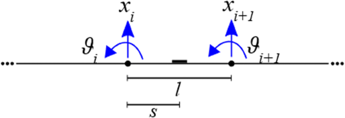
Definition of the sensed strain

The two strain gauges have been placed at 175 mm from the free-end of the beam since this location ensures a good observability and a good signal-to-noise ratio, in particular for the vibrational mode of interest.
-
a laser doppler vibrometer to get direct measurement of the velocity of a point near the free end of the beam, which is the part of the system that vibrates the most.
Other sensor configurations could be adopted provided that they ensure adequate system observability.
In the light of all the critical issues discussed in Section 5, an accurate tuning of the state observer has been performed in this experimental campaign both through a wise synthesis of the system model and the tuning of the state observer gain.
Since the beam has negligible effect on the slip-table, the table acceleration \( {\ddot{x}}_s \) has been assumed as the exogenous input for the model of the state observer, rather than force fA driving the slip-table (which is also difficult to measure). \( {\ddot{x}}_s \) has been measured through an ICP accelerometer placed on the moving table (see Fig. 1). Hence, the state-space model for the observer synthesis, that fits the one in (18) is the following one:
Model reduction has been then performed by retaining the 2 lowest-frequency vibrational modes (i.e. retaining 4 coordinates in the reduced order model), while discarding the 5 higher frequency ones. A first-order, low-pass filter with a cut-off frequency at 350 Hz has been also adopted to further reduce observation spillover.
As for the observer gain matrix L (see (24)), it has been computed through the Kalman’s theory as follows:
Matrix P is the solution of the time-infinite Riccati’s equation, matrices Q and R are parameters representing the expected measurement and process noise covariance matrices:
The sampling time adopted is 1 ms, for trading-off between the needs of high-rate control and estimation, numerical stability and low computational effort, while the numerical integration of the differential equations of the state observer has been done by means of the explicit 4th order Runge-Kutta scheme.
An example of the effectiveness of the estimator is shown in Fig. 9, which compares the estimated and the actual values measured by the vibrometer (upper figure) and the strain (lower figure) during a frequency sweep (only an excerpt is shown to provide a clearer representation). The measured and the estimated signals are almost overlapped, and the estimation error is negligible. Additionally, it can be noticed that the state observer filters measurement noise, such as for example the spike recorded in the speed measurement at about time 1.3 s, thanks to the model used in the prediction phase.

Comparison of actual and estimated quantities
All these choices lead to an expected natural frequency of the desired mode that is 49.9 Hz, as computed through the model in (28). The same model reveals that the cosine between the theoretical expected eigenvector (i.e. the one assuming feedback of the actual and full state vector, computed through the corrected model that includes moment of inertia of the added masses) and the one perturbed by the observer (i.e. the one computed through the dynamic matrix in (28)) is higher than 0.9999 for both the real and the imaginary part. The differences with respect to the target values (i.e. without observer and with the full order model) are clearly negligible and therefore the choice of the reduced model has negligible impact on the overall solution. Hence, the proposed methodology is an effective approach for the integrated design and for forecasting the effect of the state observer.
6.6.1 Experimental assessment of the eigenstructure assignment
The control gains have been computed through the method proposed by Ram and Mottershead (2007), and subsequently extended in Ouyang (2011) and Ouyang et al. (2013) for asymmetric systems, which provides an effective and reliable solution for the case of rank-one control. However, any method could be used.
The experimental results obtained show that the control scheme employed succeeded in boosting the achievement of the control specifications. Indeed, the desired mode shape of the closed-loop pole at 50 Hz is very close to the desired one. Figure 10 shows the mode shape identified experimentally (only the translational components of the eigenvector has been identified, and hence it is represented with a linear interpolation) and compares it with the desired one. The cosine of the angle between the obtained mode and the desired one is 0.966. This is an excellent result that approximates very tightly the theoretical expectations. The difference is mainly due to the approximation of the lumped masses through two masses with finite moment of inertia (as already discussed and shown in Fig. 7) and to the unavoidable presence of unmodeled and uncertain dynamics (especially because of the piezoelectric actuator and his nonlinearities and deviation from the ideal model). Indeed, the cosine of the angle between the experimental mode and the best achievable eigenvector, i.e. the “numerical with actual model” depicted through a black line in Fig. 11, is 0.997. This result fits very closely the theoretical expectations since the cosine between the best achievable eigenvector and the one computed from the augmented model in (28), which included the controlled system and the observer, is 0.999. Hence, just a negligible downgrade of the result (i.e. from 1 to 0.999) is due to the observer because of a wise design of the observer itself, that has allowed reducing spillover. Again, this result proves that the observer and the reduced model has negligible impact on the overall solution, due to a wise synthesis of the observer in accordance with the theory proposed in Section 5.1.

Comparison between the desired mode and the one obtained experimentally (cosine between the two vectors: 0.966)

Analysis of the spillover effects with hybrid control: comparison between the theoretical expected eigenvector (with actual state feedback) and the one obtained experimentally (cosine between the two vectors: 0.997)
Table 3 summarizes the cosine improvement due to the proposed hybrid control, by comparing the main results of the numerical and experimental investigation. Overall, a great improvement has been obtained, by proving the effectiveness of theory developed and of the comprehensive method proposed, that includes the synthesis of the controller, of the observer and of the physical modifications.
7 Conclusions
This paper introduced a hybrid method for structural optimization through eigenstructure assignment in an active cantilever beam by exploiting the concurrent design of the physical modifications of the system elastic and inertial parameters, and the synthesis of the state-feedback controller. The optimal physical modifications shape the allowable subspace in such a way that it spans a closer approximation of the desired eigenvector compared with the one achievable by the original system. The method is suitable for underactuated systems, such as the studied one, where the size of the set of achievable eigenvectors makes EA challenging: the concurrent use of both the techniques overcome the limitations of the use of either passive modifications or active control alone, by enlarging the set of assignable eigenpairs.
The optimal solution is computed by solving a rank-minimization problem with constraints on the design variables, that arises from the definition of the allowable subspace. A convex optimization problem is formulated through the semidefinite embedding lemma and the so-called trace heuristics, and reliable numerical solution can be performed.
The paper covers all the issues for the implementation of this control approach in a real system, including the synthesis of a state observer for replacing the actual state with the estimated one. The use of a reduced-order observer, to allow for real time computation, causes spillover of the closed-loop poles and perturbation of the mode shapes that might severely downgrade the achievable performances. A model to cope with this issue is therefore presented and the coupling with the controller is shown.
The experimental results obtained are very satisfactory. First of all, the proposed method succeeded in achieving a tight approximation of the desired performances both in terms of mode shape and natural frequency: the cosine between the desired mode shape and the achieved one is 0.966, while active control alone leads to 0.524. Secondly, the theoretical expectations closely fit the experimental results, thanks to a careful design of the state observer introducing negligible perturbation of the desired eigenpair: the perturbation due to the observer is small and the cosine between the expected eigenvector and the one obtained in the testbed is 0.997.
References
Andry AN, Shapiro EY, Chung JC (1983) Eigenstructure assignment for linear systems. IEEE Trans Aerosp Electron Syst 5:711–729
Araújo JM, Dórea CE, Gonçalves LM, Datta BN (2016) State derivative feedback in second-order linear systems: a comparative analysis of perturbed eigenvalues under coefficient variation. Mech Syst Signal Process 76:33–46
Aydin E, Dutkiewicz M, Öztürk B, Sonmez M (2020). Optimization of elastic spring supports for cantilever beams. Struct Multidiscip Optim 62:55–81. https://doi.org/10.1007/s00158-019-02469-3
Belotti R, Richiedei D (2018) Dynamic structural modification of vibrating systems oriented to eigenstructure assignment through active control: a concurrent approach. J Sound Vib 422:358–372
Belotti R, Richiedei D, Trevisani A (2016) Optimal design of vibrating systems through partial eigenstructure assignment. J Mech Des 138(7):071402 (8 pages)
Belotti R, Richiedei D, Trevisani A (2017) Concurrent design of active control and structural modifications for eigenstructure assignment on a cantilever beam. In ASME 2017 International design engineering technical conferences and computers and information in engineering conference. American Society of Mechanical Engineers Digital Collection
Belotti R, Caracciolo R, Palomba I, Richiedei D, Trevisani A (2018a) An updating method for finite element models of flexible-link mechanisms based on an equivalent rigid-link system. Shock Vib 2018:1–14. https://doi.org/10.1155/2018/1797506
Belotti R, Ouyang H, Richiedei D (2018b) A new method of passive modifications for partial frequency assignment of general structures. Mech Syst Signal Process 99:586–599
Belotti R, Richiedei D, Tamellin I (2020) Antiresonance assignment in point and cross receptances for undamped vibrating systems. J Mech Des 142(2):022301 (7 pages. https://doi.org/10.1115/1.4044329
Caracciolo R, Richiedei D, Trevisani A (2008) Robust piecewise-linear state observers for flexible link mechanisms. J Dyn Syst Meas Control 130(3). https://doi.org/10.1115/1.2909600
Corr LR, Clark WW (2002) Active and passive vibration confinement using piezoelectric transducers and dynamic vibration absorbers. J Mech Behav Mater 13(2):117–134
Delissen A, van Keulen F, Langelaar M (2020) Efficient limitation of resonant peaks by topology optimization including modal truncation augmentation. Struct Multidiscip Optim 61:2557–2575. https://doi.org/10.1007/s00158-019-02471-9
Fazel M, Hindi H, Boyd SP (2001) A rank minimization heuristic with application to minimum order system approximation. In Proceedings of the 2001 American Control Conference 6:4734–4739
Fazel M, Hindi H, Boyd SP (2003) Log-det heuristic for matrix rank minimization with applications to Hankel and Euclidean distance matrices. In Proceedings of the 2003 American Control Conference 3:2156–2162
Franklin GF, Powell JD, Emami-Naeini A, Sanjay HS (2015) Feedback control of dynamic systems. Pearson, London
Gaudenzi P, Carbonaro R, Benzi E (2000) Control of beam vibrations by means of piezoelectric devices: theory and experiments. Compos Struct 50(4):373–379
Hauser BR, Wang BP (2018) Optimal design of a parallel beam system with elastic supports to minimize flexural response to harmonic loading using a combined optimization algorithm. Struct Multidiscip Optim 58(4):1453–1465
Hehenberger P, Follmer M, Geirhofer R, Zeman K (2013) Model-based system design of annealing simulators. Mechatronics 23(3):247–256
Hernandes JA, Suleman A (2014) Structural synthesis for prescribed target natural frequencies and mode shapes. Shock Vib, Article ID 173786 2014 https://doi.org/10.1155/2014/173786
Jihong Z, Weihong Z (2006) Maximization of structural natural frequency with optimal support layout. Struct Multidiscip Optim 31(6):462–469
Kim Y, Kim HS, Junkins JL (1999) Eigenstructure assignment algorithm for mechanical second-order systems. J Guid Control Dyn 22(5):729–731
Lee J (2019) Multi-objective optimization case study with active and passive design in building engineering. Struct Multidiscip Optim 59(2):507–519
Moore B (1976) On the flexibility offered by state feedback in multivariable systems beyond closed loop eigenvalue assignment. IEEE Trans Autom Control 21(5):689–692
Ouyang H (2011) A hybrid control approach for pole assignment to second-order asymmetric systems. Mech Syst Signal Process 25(1):123–132
Ouyang H, Richiedei D, Trevisaniv AV (2013) Pole assignment for control of flexible link mechanisms. J Sound Vib 332(2013):2884–2899
Palomba I, Richiedei D, Trevisani A (2015) Energy-based optimal ranking of the interior modes for reduced-order models under periodic excitation. Shock Vib 2015:1–10. https://doi.org/10.1155/2015/348106
Palomba I, Richiedei D, Trevisani A (2017) Kinematic state estimation for rigid-link multibody systems by means of nonlinear constraint equations. Multibody Syst Dyn 40(1):1–22
Preumont A (2011) Vibration control of active structures, an introduction, 3rd edn. Springer International Publishing, Cham. https://doi.org/10.1007/978-94-007-2033-6
Ram YM, Mottershead JE (2007) Receptance method in active vibration control. AIAA J 45(3):562–567
Richiedei D, Trevisani A (2017) Simultaneous active and passive control for eigenstructure assignment in lightly damped systems. Mech Syst Signal Process 85:556–566
Richiedei D, Tamellin I, Trevisani A (2019) A general approach for antiresonance assignment in undamped vibrating systems exploiting auxiliary systems. In: Uhl T (ed) Advances in mechanism and machine science. IFToMM WC 2019. Mechanisms and machine science, vol 73. Springer, Cham, pp 4085–4094. https://doi.org/10.1007/978-3-030-20131-9_407
Richiedei D, Tamellin I, Trevisani A (2020) Simultaneous assignment of resonances and antiresonances in vibrating systems through inverse dynamic structural modification. J Sound Vib 485, 27 October 2020, 115552:19. https://doi.org/10.1016/j.jsv.2020.115552
Sanjurjo E, Dopico D, Luaces A, Naya MÁ (2018) State and force observers based on multibody models and the indirect Kalman filter. Mech Syst Signal Process 106:210–228
Schulz MJ, Inman DJ (1994) Eigenstructure assignment and controller optimization for mechanical systems. IEEE Trans Control Syst Technol 2(2):88–100
Tang J, Wang KW (2004) Vibration confinement via optimal eigenvector assignment and piezoelectric networks. J Vib Acoust 126(1):27–36
Thomas S, Li Q, Steven G (2020) Topology optimization for periodic multi-component structures with stiffness and frequency criteria. Struct Multidiscip Optim 61:2271–2289. https://doi.org/10.1007/s00158-019-02481-7
Triller MJ, Kammer DC (1997) Improved eigenstructure assignment controller design using a substructure-based coordinate system. J Guid Control Dyn 20(5):941–948
Xiao M, Lu D, Breitkopf P, Raghavan B, Dutta S, Zhang W (2020) On-the-fly model reduction for large-scale structural topology optimization using principal components analysis. Struct Multidiscip Optim 62:209–230. https://doi.org/10.1007/s00158-019-02485-3
Yan K, Wang BP (2020) Two new indices for structural optimization of free vibration suppression. Struct Multidiscip Optim 61:2057–2075. https://doi.org/10.1007/s00158-019-02451-z
Zhai J, Zhao G, Shang L (2017) Integrated design optimization of structural size and control system of piezoelectric curved shells with respect to sound radiation. Struct Multidiscip Optim 56(6):1287–1304
Zhang J, Ouyang H, Yang J (2014) Partial eigenstructure assignment for undamped vibration systems using acceleration and displacement feedback. J Sound Vib 333(1):1–12
Zheng S, Zhao X, Yu Y, Sun Y (2017) The approximate reanalysis method for topology optimization under harmonic force excitations with multiple frequencies. Struct Multidiscip Optim 56(5):1185–1196
Acknowledgments
Open access funding provided by Università degli Studi di Padova within the CRUI-CARE Agreement.
Author information
Authors and Affiliations
Corresponding author
Ethics declarations
Conflict of interest
The authors declare that they have no conflict of interest.
Replication of the results
The Appendix proposes the Matlab code for the computation of the optimal structural modifications for hybrid control, by implementing the rank-minimization method in (16). It requires the toolbox YALMIP (https://yalmip.github.io). The data for replicating the test can be obtained from the description of the test rig provided in Section 6.
Additional information
Responsible Editor: Somanath Nagendra
Publisher’s note
Springer Nature remains neutral with regard to jurisdictional claims in published maps and institutional affiliations.
Appendix
Appendix

Rights and permissions
Open Access This article is licensed under a Creative Commons Attribution 4.0 International License, which permits use, sharing, adaptation, distribution and reproduction in any medium or format, as long as you give appropriate credit to the original author(s) and the source, provide a link to the Creative Commons licence, and indicate if changes were made. The images or other third party material in this article are included in the article's Creative Commons licence, unless indicated otherwise in a credit line to the material. If material is not included in the article's Creative Commons licence and your intended use is not permitted by statutory regulation or exceeds the permitted use, you will need to obtain permission directly from the copyright holder. To view a copy of this licence, visit http://creativecommons.org/licenses/by/4.0/.
About this article

Cite this article
Belotti, R., Richiedei, D. & Trevisani, A. Multi-domain optimization of the eigenstructure of controlled underactuated vibrating systems. Struct Multidisc Optim 63, 499–514 (2021). https://doi.org/10.1007/s00158-020-02709-x
Received:
Revised:
Accepted:
Published:
Issue Date:
DOI: https://doi.org/10.1007/s00158-020-02709-x