


1. Introduction
Sea ice, atmospheric and oceanic circulation patterns in the Arctic have a complex, coupled relationship that manifests across multiple spatial and temporal scales. Recent anthropogenic climate change has increased air temperatures in the Arctic at a faster rate than the global average and as such, has created a phenomenon called Arctic amplification (Serreze and Barry, Reference Serreze and Barry2011). Arctic amplification is characterized by multiple positive feedback loops associated with the redistribution of oceanic and atmospheric heat owing to the lack of a high-albedo sea ice and snow cover (Bhatt and others, Reference Bhatt2014). Furthermore, Arctic amplification has been connected to global-scale processes including alteration of the mid-latitude jet-stream and extreme weather events (Cohen and others, Reference Cohen2014), and therefore, directly affects the latitudes across which the majority of the world's population resides. Understanding the nuanced interactions among Arctic ocean-ice-atmosphere environmental systems is of utmost importance, as they play a critical role in governing weather patterns throughout the entire Northern Hemisphere.
Sea-ice cover in the Arctic has been declining in thickness, extent and seasonal duration since the late 1970s (e.g., Perovich and Richter-Menge, Reference Perovich and Richter-Menge2009; Stroeve and others, Reference Stroeve2012) and the Arctic is expected to be sea-ice-free in summer by 2030 (Overland and Wang, Reference Overland and Wang2013). These declines in sea-ice extent and thickness are known to be affected by atmospheric conditions, such as cloud cover and cloud type. Specifically, thicker spring clouds increase downward longwave radiation flux and accelerate sea-ice loss (Huang and others, Reference Huang2019). However, this presents a positive-feedback relationship whereby cloud changes may also be forced by the variability of sea ice (Francis and Hunter, Reference Francis and Hunter2006; Eastman and Warren, Reference Eastman and Warren2010). For example, across the broader Arctic, there has been a general increase in cloud cover during years with particularly low ice owing to the opportunity for increased heat exchange between an open ocean surface with the atmosphere (Eastman and Warren, Reference Eastman and Warren2010).
Local scale declines in sea ice, or increases in the duration of an open water season, serve an important role in the transfer of heat and moisture to surrounding regions (Rennermalm and others, Reference Rennermalm, Smith, Stroeve and Chu2009; Stroeve and others, Reference Stroeve2017). Specifically, declines in sea-ice cover along the coast of West Greenland, have been directly linked to increased surface melt of the ice sheet through the onshore advection of sensible and latent heat from Baffin Bay (Rennermalm and others, Reference Rennermalm, Smith, Stroeve and Chu2009; Stroeve and others, Reference Stroeve2017), and as such, sea ice plays an indirect role in increasing global sea levels. While it may remain difficult to grasp how changes in Arctic sea ice may directly influence global populations, rises in ocean temperature observed around Greenland are known to destabilize the termini of marine glaciers (Holland and others, Reference Holland and Thomas2008; Straneo and others, Reference Straneo2012), and in turn, raise global sea levels. Previous work has shown that such changes in marine glacier terminus position have a strong relationship with seasonal fjord ice mélange and sea-ice conditions, whereby a rigid winter mélange may act as a buttress inhibiting glacier flow (Joughin and others, Reference Joughin2008; Howat and others, Reference Howat, Box, Ahn, Herrington and McFadden2010; Moon and others, Reference Moon, Joughin and Smith2015). Given that ice mélange is simply a mixture of icebergs and stabilized by sea-ice formation in winter (Joughin and others, Reference Joughin2008), the future sea-ice decline indicated by projections (Overland and Wang, Reference Overland and Wang2013) may have a dramatic effect on the buttressing stability of ice mélange. Therefore, this creates the potential of increased rates of glacier terminus retreat and an indirect contribution to sea-level rise from sea-ice loss.
Around the southern tip of Greenland, there has been a documented increase in glacial meltwater discharge at the end of summer which has coincided with the occurrence of late-season phytoplankton blooms (Arrigo and others, Reference Arrigo2017; Oliver and others, Reference Oliver2018). Previous work suggests that glacial meltwater has enhanced bioavailability of the micronutrient iron (Fe) (Bhatia and others, Reference Bhatia2013). Iron in particular, has been found to be a co-limiting factor for nitrogen fixation, and hence, marine productivity and additions of the micronutrients iron and phosphorus into an ocean system have been found to stimulate production (Mills and others, Reference Mills, Ridame, Davey, La Roche and Geider2004). Nutrient availability for blooms in the Arctic has also increased owing to delays in autumnal sea-ice freeze-up, which allows for increased wind-driven vertical mixing of nitrogen and in turn, the occurrence of a secondary fall bloom (Ardyna and others, Reference Ardyna2014). While the spatial extent of nutrients from glaciers has been debated in terms of either being restricted to individual fjords (Meire and others, Reference Meire2015, Reference Meire2017) or distributed across a broader region (Arrigo and others, Reference Arrigo2017), introduction of fresh glacial meltwater into the circulation system alters water stratification and can redistribute nutrient-rich waters at depth to the surface (Arrigo and others, Reference Arrigo2017; Oliver and others, Reference Oliver2018). Changes in the timing and magnitude of primary production at the base of the food chain can trickle-up to higher trophic levels and ultimately, may impact migration patterns of larger animals, such as those that are relied on by Arctic Inuit communities for subsistence-based livelihoods.
Previous work has largely been limited to the investigation of Arctic-wide trends in sea-ice cover, sea surface temperatures, chlorophyll-a concentration and primary production or regional studies that investigated averages of only individual or couplings of these cryospheric-oceanographic systems. To gain a more holistic understanding of the ice–ocean system, in this study, we utilized multiple satellite data products to analyze timeseries of seasonal and annual sea-ice concentration, sea surface temperatures and ocean color and contextualize these in terms of broader climate indices over the 20-year period between 1998 and 2017. We focus on the Baffin Bay, Davis Strait and the Labrador Sea region located between the northeast coast of Canada and the west coast of Greenland spanning the Northwest Atlantic Ocean and Southern Arctic Ocean (Fig. 1), as it has shown dynamic oceanographic behavior in recent years (e.g., Heide-Jørgensen and others, Reference Heide-Jørgensen, Stern and Laidre2007; Frey and others, Reference Frey, Comiso, Cooper, Grebmeier and Stock2018), particularly related to the location of the southernmost winter sea-ice edge.

Fig. 1. The Baffin Bay, Davis Strait and Labrador Sea study area. Background image from the IBCAO dataset (Jakobsson and others, Reference Jakobsson2012) which we note does not extend to the southwest region of the study area.
2. Methods
2.1. Study area
Maximum bathymetric depths range from ~3000 m in the Labrador Sea, 2000 m in the central portion of Baffin Bay and 500 m in the narrow Davis Strait region that connects them (Fig. 1; Jakobsson and others, Reference Jakobsson2012). These regions are characterized by both cold Arctic water inputs from the north through the Nares Strait, Lancaster Sound (Rudels, Reference Rudels2011) and Jones Sound, as well as warmer Atlantic waters of the West Greenland Current that flow north along the west coast of Greenland (Cuny and others, Reference Cuny, Rhines and Kwok2005; Straneo and others, Reference Straneo2012). These waters converge in northern Baffin Bay and move southward as the Baffin Island Current along the east coast of Canada back into the north Atlantic (Tang and others, Reference Tang2004).
Previous work has indicated strong east-west gradients in surface air temperature in winter and less variability across the study area in summer (Tang and others, Reference Tang2004). Since the 1940s, similar magnitudes of ~2 °C surface air temperature increases have been documented in both winter and summer seasons (Peterson and others, Reference Peterson and Pettipas2015). Wind stresses in the study area also show a strong seasonal signal: summer stresses are generally weak throughout the region, while stronger stresses in the south in winter and weaker stresses in the north drive much of the movement of sea ice from Baffin Bay to the sea-ice edge in the Labrador Sea (Tang and others, Reference Tang2004). In general, this southern sea-ice edge in winter does not follow a single line of latitude, but rather crosses the Labrador Sea moving from ~55°N along the east coast of Canada northwest to ~65°N along the west coast of Greenland.
Many glaciers along the West Greenland and eastern Canadian coast outlet into this region of the Northwest Atlantic and Southern Arctic oceans. Particularly along the central west coast of Greenland, marine-terminating glaciers have shown increased velocities (Moon and others, Reference Moon, Joughin, Smith and Howat2012), increased frontal retreat (Catania and others, Reference Catania2018) and decreased surface elevation (Felikson and others, Reference Felikson2017) over recent decades. Given the potential influence of regional sea ice decline on ice-sheet surface melt (Rennermalm and others, Reference Rennermalm, Smith, Stroeve and Chu2009; Stroeve and others, Reference Stroeve2017) and ice mélange on marine-terminating glacier front stability (Joughin and others, Reference Joughin2008; Howat and others, Reference Howat, Box, Ahn, Herrington and McFadden2010; Moon and others, Reference Moon, Joughin and Smith2015), understanding sea-ice changes in our study area is of utmost importance, owing to the potential indirect influences on sea-level rise through these interactions with the Greenland ice sheet and peripheral glaciers.
2.2. Data and processing
Gaps exist in the remotely sensed data products used in the study due to cloudiness, sea-ice cover, or other satellite retrieval errors. To address the issue of missing data created by such gaps and because our study period is relatively short, we calculated trends using the nonparametric Theil–Sen median slope estimator (Sen, Reference Sen1968), which has proven robust for assessing change in these types of noisy time series (Hoaglin and others, Reference Hoaglin, Mosteller and Tukey2000; Frey and others, Reference Frey, Moore, Cooper and Grebmeier2015). We maintained a resistant statistic defined by a 29% breakdown bound (Hoaglin and others, Reference Hoaglin, Mosteller and Tukey2000), where under this rule, only those pixels that have 71% of existing data values were included in the trend calculations discussed throughout the following Data and Processing sections of the paper. Therefore, up to 29% of data in the Theil-Sen calculations can be random before the statistic breaks down. In this case, we required at least 15 years of observations and no more than five missing data values over the 20 years (1998–2017) for our calculations. Pixels with 5 years or fewer observations were masked out from analyses. Further investigation into those pixels defined as not meeting the breakdown bound requirement of minimum observations suggested there were no temporal biases in missing values or apparent clustering during particular years throughout the study period. We then tested the statistical significance (p < 0.05) of each valid pixel's trend using the nonparametric Mann–Kendall test for monotonic trends (Mann, Reference Mann1945; Kendall, Reference Kendall1975).
2.2.1. Sea ice
We used daily imagery from the Scanning Multi-channel Microwave Radiometer (SMMR), Special Sensor Microwave Imager (SSM/I) and Special Sensor Microwave Imager/Sounder (SSMIS) (25 km) passive microwave instruments carried on the Nimbus-7 satellite between 1998 and 2017. Sea-ice concentration (%) was derived using the Goddard Bootstrap SB2 algorithm (Comiso and others, Reference Comiso, Meier and Gersten2017). Remotely sensed sea-ice concentration algorithms are generally in good agreement of overall trends, however, maximum and minimum extents of Arctic sea ice calculated using the SB2 algorithm most closely matched the average extent calculated by four different sea-ice algorithms (Comiso and others, Reference Comiso, Meier and Gersten2017). Following Frey and others (Reference Frey, Moore, Cooper and Grebmeier2015), we calculated both annual and monthly sea-ice persistence as the summed number of days within a year or month, respectively, for which a pixel was determined as present based on the standard 15% threshold (Cavalieri and others, Reference Cavalieri, Parkinson, Gloersen and Zwally2008). Sea-ice breakup was defined as having occurred between March 15 and September 15 and the breakup day of year (DOY) was determined by the first occurrence a pixel was calculated as having sea ice absent (<15%) for 2 consecutive days (Frey and others, Reference Frey, Moore, Cooper and Grebmeier2015). Similarly, sea-ice freeze-up was defined as occurring between September 15 and March 15 of consecutive years, and freeze-up DOY was determined by the first occurrence a pixel registered 2 consecutive days of sea-ice presence (>15%) (Frey and others, Reference Frey, Moore, Cooper and Grebmeier2015). While freeze-up is more of a synoptic climatological process in this region, we note that sea ice may become present again after the assigned break-up date under this rule; however, this rule serves as a good estimate of when a sea-ice pixel transitions into the annual break-up phase based on the seasonal progression observed through the monthly persistence calculations. We calculated the spatial trends in the three different sea-ice conditions using the nonparametric Theil–Sen median slope estimator (Sen, Reference Sen1968) and tested the statistical significance (p < 0.05) of each trend using the nonparametric Mann–Kendall test for monotonic trends (Mann, Reference Mann1945; Kendall, Reference Kendall1975).
Finally, we calculated the linearly detrended Pearson's correlation coefficients (R) between the mean summer (JAS) and winter (JFM) Arctic Oscillation (AO) Index, the North Atlantic Oscillation (NAO) Index (http://www.cpc.ncep.noaa.gov/), and the Greenland Blocking Index (GBI) (https://psl.noaa.gov/data/timeseries/daily/GBI/; Hanna and others, Reference Hanna, Cropper, Hall and Cappelen2016), with the total days of sea-ice persistence over the same seasonal months.
2.2.2. Sea surface temperatures and ocean color
For the three open-ocean phenomena: sea surface temperature, chlorophyll-a concentration and primary productivity, we chose to focus on the months of March–September for which there was sufficient data owing to decreased sea-ice cover and increased sunlight, as well as being the time of year when we observed the majority of change in these ocean variables between 1998 and 2017. It is important to note that these serve as only estimates of monthly averages, taken under clear-sky and open-ocean conditions. As described above, by maintaining the 29% breakdown bound, only those pixels with at least 15 years of observations over the study period were included in monthly trend calculations and pixels with five or fewer years of valid data were masked out.
Sea surface temperature (SST; °C) monthly averages were calculated using the daily Optimum Interpolation Sea Surface Temperature dataset (OISSTv2). This dataset combines in-situ observations with satellite measurements from the Advanced Very High-Resolution Radiometer (AVHRR) instrument (Reynolds and others, Reference Reynolds2007).
Chlorophyll–a monthly concentrations (mg m–3) were derived from a combination of the Sea-Viewing Wide Field-of-View Sensor (SeaWiFS) (1997–2010) and Aqua Moderate Resolution Imaging Spectroradiometer (Aqua MODIS) (2003–17) data utilizing the OCx band ratio algorithm (O'Reilly and others, Reference O'Reilly1998) combined with the color index of Hu and others (Reference Hu, Lee and Franz2012), available from the NASA Goddard Space Flight Center Ocean Biology Processing Group. To create the hybrid time series, Aqua MODIS data were calibrated to SeaWiFS data by applying a linear regression across the Arctic region for corresponding data, with subsequent averaging of values where coincident data occurred. Chlorophyll–a monthly averages solely reflect clear-sky (i.e., based on the embedded cloud mask associated with the ocean color data) and ice-free (i.e., <15% sea-ice concentration) conditions (e.g., Smith and Comiso, Reference Smith and Comiso2008).
Net primary productivity (gC m–2) monthly estimates between 1998 and 2017 were derived from the AVHRR SST and SeaWiFS/MODIS chlorophyll-a data described above, as well as photosynthetically active radiation (PAR) extracted as part of the SeaWiFS/MODIS data (provided by J. Comiso and L. Stock, NASA Goddard). The equation for the calculation of primary productivity, described in detail in Smith and Comiso (Reference Smith and Comiso2008), is based on temperature's control on the rate of photosynthesis within the water column estimated using the AVHRR SST in the polynomial equation described in Behrenfeld and Falkowski (Reference Behrenfeld and Falkowski1997), as well as the daily surface PAR and surface chlorophyll-a concentration determined from SeaWiFS/MODIS. Finally, for each pixel with at least 15 years of data, we calculated the monthly Theil-Sen trends and the Mann–Kendall significance (p < 0.05) of the three open-ocean phenomena: SST, chlorophyll–a, and primary productivity.
3. Results
3.1. Sea-ice persistence
Based on climatology, sea ice was present within the study region from November through July (Fig. 2). We found a positive trend in the days per month sea-ice persisted along the sea-ice edge in the majority of winter months (Fig. 3). Specifically, there were positive trends along the western edge of Greenland in December and along southeastern Canada in March, April and May. However, we also saw a significant negative trend in the number of days sea ice was present in northern Baffin Bay in June and central Baffin Bay in July. On average, sea ice persisted for >180 days in the northwest portion of the study area along Baffin Island, and ~30–60 days along the southeastern sea-ice edge (Fig. 4a). Similarly, annual sea-ice persistence showed significant positive trends in the western Labrador Sea of ~5 days a–1, while there were significant decreases of ~3 days a–1 throughout the northern portion of the study area in Baffin Bay (Fig. 5a).

Fig. 2. Mean monthly sea-ice persistence (days per month) based on 15% presence/absence threshold.

Fig. 3. Thiel-Sen median trends in monthly sea-ice persistence (days per month). Hatching indicates significant trends (p < 0.05) using the Mann–Kendall test.

Fig. 4. (a) Mean annual sea-ice persistence (days a–1); (b) mean timing of sea-ice break-up (DOY) between 15 March and 15 September; (c) mean timing of sea-ice freeze-up (DOY) between 15 September and 15 March.

Fig. 5. Thiel-Sen median (a) trends in annual sea-ice persistence (days a–1); (b) trends in the timing of sea-ice break-up (days a–1); (c) trends in the timing of sea-ice freeze-up (days a–1). Hatching indicates significant trends (p < 0.05) using the Mann–Kendall test.
We found a significant positive correlation (p < 0.05) with both the AO and the NAO and monthly sea-ice persistence along the southernmost sea-ice edge in winter (JFM) (Figs 6b and e). Summer (JAS) monthly sea-ice persistence also showed a significant negative correlation with the AO along the east coast of Baffin Island (Fig. 6a). Opposite to the relationship between sea-ice persistence and the AO and NAO, we also found a significant positive correlation with the GBI along eastern Baffin Island in summer and a significant negative correlation along the southern sea-ice edge with the GBI in winter (Figs 6c and f).
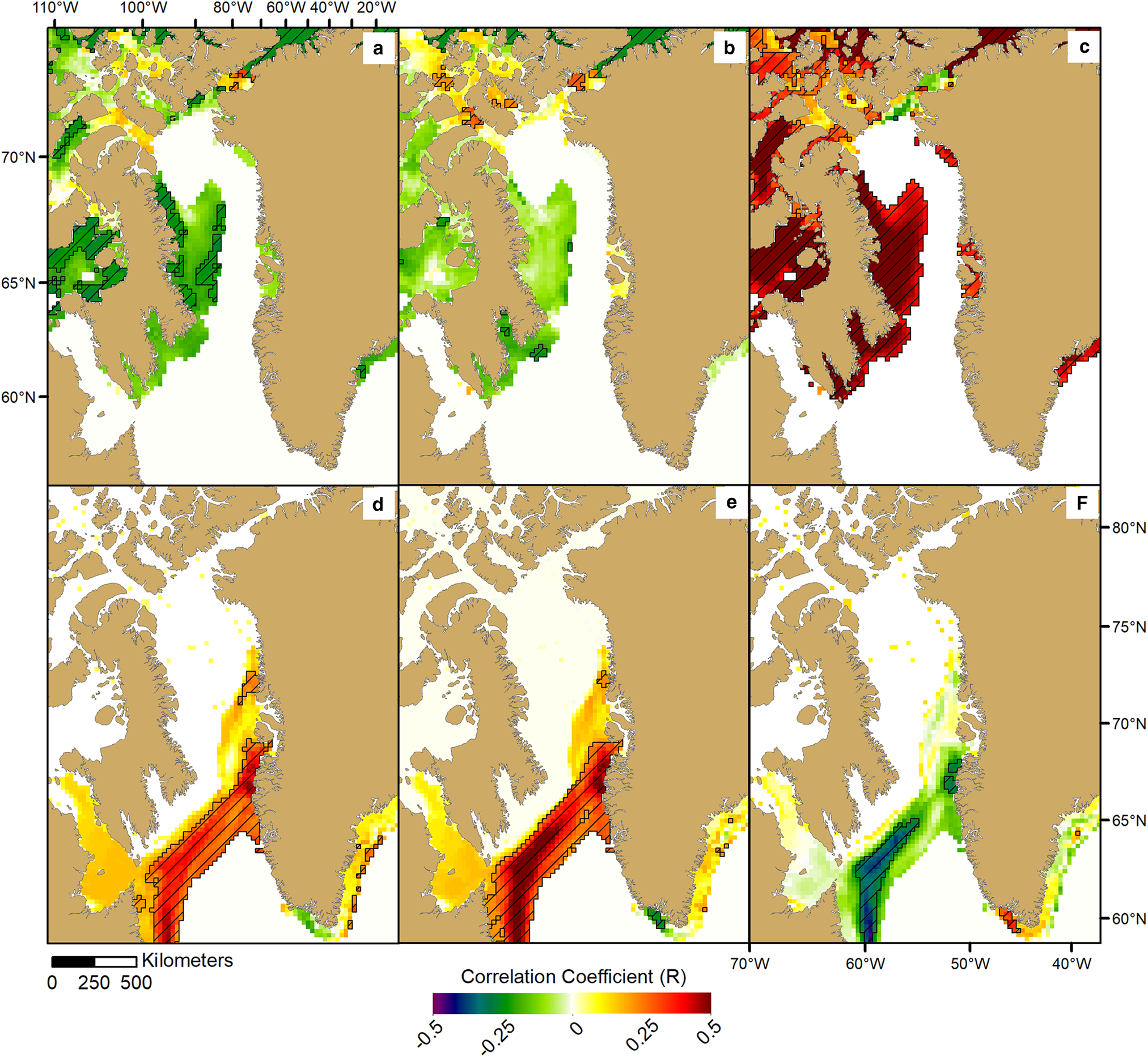
Fig. 6. Detrended correlation coefficients (R) calculated between monthly summer (JAS) and monthly winter (JFM) sea-ice persistence (days per month) and the Arctic Oscillation (AO) and North Atlantic Oscillation (NAO) climate indices, as well as the Greenland Blocking Index (GBI) (Hanna and others, Reference Hanna, Cropper, Hall and Cappelen2016). (a) Summer sea-ice persistence and the AO; (b) summer sea-ice persistence and the NAO; (c) summer sea-ice persistence and the GBI; (d) winter sea-ice persistence and the AO; (e) winter sea-ice persistence and the NAO; and (f) winter sea-ice persistence and the GBI. Hatching indicates significant trends (p < 0.05).
3.2. Sea-ice break-up and freeze-up
Sea-ice freeze-up (defined by our algorithm to be restricted to 15 September–15 March 15) generally began in October in the northwest Baffin Bay and advanced to the southeast Labrador Sea where formation generally occurred in February (Fig. 4c). Spring sea-ice break-up (defined as occurring between 15 March and September 15) generally followed the reverse path of freeze-up progression, beginning in the southeast in May and progressing northwestward with the latest sea-ice break-up taking place along the east coast of Baffin Island in July (Fig. 4b). This reinforces our monthly sea-ice persistence observations of the southernmost sea-ice edge in March and April and lack of sea ice during August–October. The significant negative trends in persistence that occurred in Baffin Bay are primarily because of the earlier sea-ice break-up, as we observed a significant change of ~2 days a–1 and only a small area of significant later sea-ice freeze-up (Figs 5b and c). Yet, we also observed significant trends towards later sea-ice break-up of ~1 day a–1 along the southwestern edge and significant earlier freeze-up of ~1 day a–1 near Disko Island. These break-up and freeze-up observations account for some of the spatial variability in the trends of annual sea-ice persistence (Fig. 6a).
3.3. Sea surface temperatures
On average sea surface temperature ranged from −1 to + 7 °C and exhibited both a strong positive north-south and west-east gradient (Fig. 7). Colder waters generally followed the sea-ice edge decay beginning in March and ultimately reached the highest ocean temperatures throughout the study area in August. Opening of the North Water Polynya became apparent in May when sea surface temperatures in this area are first detected. We found small areas of significant decreases in sea surface temperatures along the southwestern sea-ice edge in April and May, associated with the increased sea-ice edge persistence we observed in these months (Fig. 8). However, we observed areas of significantly increased sea surface temperatures in all months between March and September, particularly in the southeast portion of the Labrador Sea study area along the west coast of Greenland. There was a distinct west-east difference in April–June, potentially pointing to increased influence of the Irminger Current over recent decades (Holland and others, Reference Holland and Thomas2008). In summer (JAS), we found significant positive trends in sea surface temperature of 0.2 °C a–1 across the entire study area, with the largest increase over the period occurring in central Baffin Bay in July and August. The small area in Disko Bay, West Greenland showed the largest increases in sea surface temperature in July of >0.5 °C a–1. Also, during these summer months, there was a consistent area along the southeast coast of Greenland that showed significant negative trends in sea-surface temperature.

Fig. 7. Mean monthly sea surface temperatures (SSTs; °C) for March–September.

Fig. 8. Thiel-Sen median trends in monthly sea surface temperatures (SSTs; °C) for March–September. Hatching indicates significant trends (p < 0.05) using the Mann–Kendall test.
3.4. Ocean color
We observed the highest mean chlorophyll-a concentration (mg m–3) in May, southeast of the sea-ice edge and along the west coast of Greenland (Fig. 9). Despite on average having a high chlorophyll-a concentration in April relative to other months, we found a significant negative trend in these concentration over 1998–2017 (Fig. 10). Proximal to the location where we observed this negative trend in concentration in April, we see a subsequent significant positive trend in chlorophyll-a concentration in May in the eastern Labrador Sea. In June, we observed a small area of increased chlorophyll-a concentration in the Labrador Sea, as well as a decreasing chlorophyll-a concentration in the North Water Polynya. Significant positive trends in concentration of ~0.03 mg m–3 a–1 occurred in September across the majority of the Labrador Sea.

Fig. 9. Mean monthly chlorophyll-a concentration (mg m–3) for March–September.
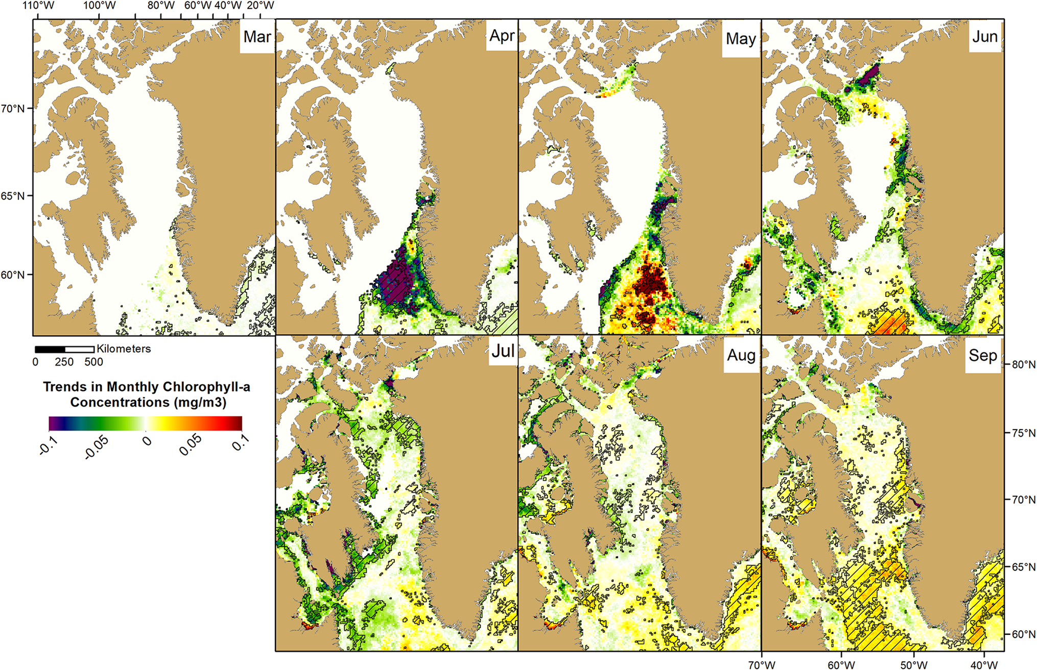
Fig. 10. Thiel-Sen median trends in monthly chlorophyll-a concentration (mg m–3) for March–September. Hatching indicates significant trends (p < 0.05) using the Mann–Kendall test.
Similar to chlorophyll-a concentration, the highest average estimates of primary production (gC m–2) over the 1998–2017 study period occurred in May along the west coast of Greenland (Fig. 11). Trends indicated significant decreases in primary production in April in the Labrador Sea and in June in the North Water Polynya (Fig. 12). However, proximal to this same location within the Labrador Sea that underwent negative trends in April, primary production significantly increased in both May and June. As seen with chlorophyll-a concentration, primary production also showed significant positive trends of ~10 gC m–2 a–1 in September across the majority of the study region.

Fig. 11. Mean monthly primary production (gC m–2) for March–September.

Fig. 12. Thiel–Sen median trends in monthly primary production (gC m–2) for March–September. Hatching indicates significant trends (p < 0.05) using the Mann–Kendall test.
4. Discussion and conclusions
4.1. Sea ice
We observed spatial variability in the trends of annual sea-ice persistence owing to declines in persistence in northern Baffin Bay and increasing persistence causing later spring break-up along the southern sea-ice edge in the Labrador Sea. Observations of positive trends in sea-ice persistence in recent years are anomalous relative to the Arctic-wide trends of sea ice, which is generally declining in thickness, extent and seasonal cover (Stroeve and others, Reference Stroeve2012). However, we observed a large region of significant decreased sea-ice persistence in central and northern Baffin Bay, with the majority of this change caused by earlier spring break-up. As such, we suggest that once break-up had been initiated along the southernmost sea-ice edge, the rate of the northward progression increased over the 1998–2017 period. Using an algorithm based on emissivity to detect melt and freeze onset, Markus and others (Reference Markus, Stroeve and Miller2009) also found significant trends of ~3 days decade–1 of sea ice shifting towards both later fall freeze-up and earlier spring break-up, when regionally averaged across Baffin Bay, Davis Strait and Labrador Sea region between 1979 and 2007. However, using the same algorithm with an extended record from 1979 to 2013, Stroeve and others (Reference Stroeve and Markus2014) found that while the trend towards earlier spring break-up increased to 4.6 days decade–1, the trend of later fall freeze-up was closer to 1 day decade–1. Ballinger and others (Reference Ballinger2018b) found sea-ice melt onset in this region occurred 8 days decade–1 earlier from 1979 to 2015, specifically linking the GBI to an anomalous 2013 melt onset event which occurred almost 50 days earlier than average. Here, by using a different methodology than previous work on melt and freeze onset studies (e.g. Markus and others, Reference Markus, Stroeve and Miller2009; Stroeve and others, Reference Stroeve and Markus2014; Ballinger and others, Reference Ballinger2018b), we shed light on local variability in sea ice across this region of the Northwest Atlantic-Southern Arctic Oceans. Specifically, we found a significant positive correlation between the GBI and sea-ice persistence along the east coast of Baffin Island in summer (JAS), and a significant negative correlation between the GBI and sea-ice persistence along the southern sea-ice edge in winter (JFM) (Fig. 6c). This is generally in agreement with the findings of Hanna and other (Reference Hanna, Cropper, Hall and Cappelen2016), who investigated the monthly and seasonal GBI between 1851 and 2015. They found the largest increases in GBI values occurred in July and August, in addition to a more recent clustering of high GBI values since 2007 (Hanna and others, Reference Hanna, Cropper, Hall and Cappelen2016). Variability in GBI values also increased in May and December, which the authors suggest is similar behavior observed in the NAO (Hanna and others, Reference Hanna, Cropper, Hall and Cappelen2016). Correlations have also been found between the timing of freeze onset with both ocean surface and atmospheric temperatures across the study region. Specifically, later fall freeze-up in Baffin Bay was found to be significantly correlated with surface air temperatures in autumn months (Ballinger and others, Reference Ballinger2018a). Here, we have shown the spatial trends of both seasonal and annual sea-ice persistence, break-up and freeze-up, in order to attribute the overall decline in sea-ice persistence in this region between 1998 and 2017. We found the majority of the region underwent negative trends in sea ice, dominated by earlier spring break-up in Baffin Bay, despite the anomalous trends of increased persistence along the southern sea-ice edge in the Labrador Sea (Fig. 5). Finally, we found sea-ice persistence across the study area was significantly correlated with multiple climate indices (AO, GBI, NAO), suggesting variability in the associated atmospheric circulation patterns may play a driving role in the timing of fall sea-ice freeze-up and spring sea-ice break-up.
Rigor and others (Reference Rigor, Wallace and Colony2002) calculated that ~64% of Arctic sea-ice concentration variance could be explained by the AO. In the past, the AO has shown a strong correlation with Northern Hemisphere surface air temperatures, until the 1990s when the rate of warming increased and the AO index became increasingly negative: a divergence Nagato and Tanaka (Reference Nagato and Tanaka2012) suggestion was caused by Arctic Amplification. Stern and Heide-Jørgensen (Reference Stern and Heide-jørgensen2003) found that the present year's NAO index could be used to predict the following winter's sea-ice concentration in Davis Strait. Specifically in the Labrador Sea, previous studies pointed to the existence of a positive correlation between the extent of the southernmost winter sea-ice edge and the winter index of the AO and the NAO over the 1979–2002 period (Heide-Jørgensen and others, Reference Heide-Jørgensen, Stern and Laidre2007). As identified by previous work in this region, we also found the strong positive relationship between these broader climate indices and the southernmost winter sea-ice edge continued between 1998 and 2017. Surface winds associated with fluctuation of the AO impacts sea-ice motion, and this motion in turn affects not only regional surface air temperatures, but also the thickness and extent of the sea ice itself (Rigor and others, Reference Rigor, Wallace and Colony2002). Wang and others (Reference Wang, Mysak and Ingram1994) found that specifically westerly winds associated with the NAO lead to negative anomalies in surface air temperature, and in turn, positive anomalies in sea ice across the Baffin Bay and Labrador Sea region. Wind may provide an efficient mechanism to drive the southward movement of thinner, annually formed ice that we observed here as the strong positive relationship between increases in sea-ice concentration along the southernmost sea-ice edge in the Labrador Sea with the winter index of the AO and NAO. These findings point to a particularly complex relationship between the recent trends in air temperature, climate indices, and sea-ice concentration and as feedbacks associated with Arctic warming continue to take place, such a direct climate index–sea-ice relationship may become increasingly less predictable in the future.
4.2. Sea surface temperatures and ocean color
In agreement with previous studies on this region (e.g. Ballinger and others, Reference Ballinger2018a), we found significant positive trends in sea surface temperatures, with the greatest trends occurring in August and September in central Baffin Bay. During the summer months (JAS), we observed a consistent area along the southeast coast of Greenland that showed significant negative trends in sea surface temperature, which may be a signal of increased meltwater runoff from regional marine-terminating glaciers. The micronutrient iron (Fe) is a known co-limiting factor on nitrogen fixation, and therefore, on primary production (Mills and others, Reference Mills, Ridame, Davey, La Roche and Geider2004). As such, it has been suggested that iron inputs from the increased glacial meltwater runoff in summer months may provide enough bioavailable iron to stimulate a secondary bloom (Bhatia and others, Reference Bhatia2013; Arrigo and others, Reference Arrigo2017). Other research has suggested such nutrient transport may be more spatially limited, and primary production associated with glacial meltwater input occurs only at the individual fjord-scale of marine-terminating glaciers in Greenland (Meire and others, Reference Meire2015, Reference Meire2017). By utilizing time series analysis to display the spatial trends in both of these oceanographic factors, this study was able to show coincident decreases sea surface temperature potentially from glacial meltwater runoff, while also showing increased chlorophyll-a and primary production in the Labrador Sea in September. A fall bloom in the Arctic such as this has also been attributed to seasonal sea-ice changes. For example, Ardyna and others (Reference Ardyna2014) suggested that delayed sea-ice freeze-up in autumn allowed for enough increased wind-driven vertical mixing of nutrients to initiate a secondary bloom. However, investigating at the regional-scale, here, we found trends moved towards earlier rather than later fall freeze-up along the southeastern sea-ice edge. The increased September chlorophyll-a and primary production observed in the Labrador Sea region by this study is therefore unlikely to have been caused by later sea-ice freeze-up. In combination with observed decreases in summer sea surface temperature along the Greenland coast, our observations point more towards glacial meltwater as a viable nutrient source for bloom initiation at this time of year, such as found by previous studies (e.g. Bhatia and others, Reference Bhatia2013; Arrigo and others, Reference Arrigo2017).
In addition to our findings that indicated the occurrence of a secondary fall bloom, we found an apparent shift in the timing towards a later spring bloom, with negative trends of both chlorophyll-a and primary production in April, followed by positive trends in May. Previous studies have also indicated that on average, April and May are the peak months for chlorophyll-a and primary production in the Labrador Sea (Wu and others, Reference Wu, Platt, Tang and Sathyendranath2008; Arrigo and others, Reference Arrigo2017) and our study elucidates the long-term trends and spatial variability of these ocean color phenomena. Perrette and others (Reference Perrette, Yool, Quartly and Popova2011) suggested that chlorophyll-a blooms can occur up to 100 km from the ice edge as it retreats northward across the Arctic in spring. However, in the western Baffin Bay region specifically, they found chlorophyll-a in July closely followed the decline of the sea-ice edge as it moves northwestward towards Baffin Island, peaking after ~20 days of ice retreat (Perrette and others, Reference Perrette, Yool, Quartly and Popova2011). As such, our observation of extended persistence of sea ice along the southernmost edge in the Labrador Sea in spring, serves as a reasonable cause for delayed peaks in chlorophyll-a and primary production from April until May, as blooms would only be initiated after the northward retreat of ice began.
Over recent years, previous work has also shown that cloud cover has increased in the Arctic associated with the increased heat flux to the atmosphere from the open ocean due to decreased seasonal sea-ice cover (Bélanger and others, Reference Bélanger, Babin and Tremblay2013). Despite Arctic-wide averages of sea-ice cover decline leading to increasing light availability to the marine ecosystem, associated increases in cloud cover can dampen the primary production potential that may otherwise be expected (Bélanger and others, Reference Bélanger, Babin and Tremblay2013). In general, total cloud cover appears to be greater within years of lower sea-ice concentration (Eastman and Warren, Reference Eastman and Warren2010). Modeled summer (JJA) cloud content (%) by Noël and others (Reference Noël, Jan van de Berg, Lhermitte and van den Broeke2019), suggests spatial variability, with decreased cloud content over the southern portion of the Greenland ice sheet and increased cloud cover in the northwest sector of the ice sheet owing to warm air advection from Baffin Bay. Their findings indicate this increased cloud cover subsequently increased downward longwave radiation, leading to observations of increased runoff by this northwest region of the ice sheet between 1991 and 2017 (Noël and others, Reference Noël, Jan van de Berg, Lhermitte and van den Broeke2019). Here, we found the majority of the Baffin Bay study region underwent declines in sea-ice persistence, primarily owing to earlier spring break-up. Furthermore, we found sea ice in Baffin Bay had a significant positive relationship with the GBI in summer (JAS). Such a lack of Baffin-wide ice cover offers the possibility for a longer season of opportunity for increased heat flux from the open ocean to increase cloudiness during spring, and therefore, increase downward longwave radiation that contributes to regional Greenland ice sheet surface melt. This ice/ocean/atmosphere relationship also holds true in the Labrador Sea, where we found a trend of increased sea-ice persistence had a significant negative correlation with the GBI and Noël and others (Reference Noël, Jan van de Berg, Lhermitte and van den Broeke2019) found regional decreases in cloud content and decreased contribution from the southern region of Greenland to total ice sheet runoff. Our research suggests this ice-ocean-atmosphere variability is also contributing to changes in oceanic biology and serves as a contributor towards the chlorophyll-a and primary production trends observed by this study in April and May over the 1998–2017 period.
Extracted time series of primary production (gC m–2) from a sample area of significant negative/positive trends in April/May point to the observed increases in May having been largely attributable to anomalously high primary production values in 2014 and 2015 (Fig. 13). Upon further look into sea-ice behavior in the same sample area, we also found a greater number of days of monthly sea-ice persistence in April of 2014 and 2015. Specifically, 2014 and 2015 April sea-ice persistence in the sample region was >20 days, compared to an average of ~4 days over the 1998–2017 study period. Previous work has shown that the winters of 2013/14 through 2015/16 were characterized by anomalously cold air masses and subsequent ocean cooling, resulting in increased production of denser Labrador Sea Water (Rhein and others, Reference Rhein2017). Colder ocean-atmosphere conditions lend cause towards the observed increased in April sea-ice persistence in 2014 and 2015. Furthermore, we found the sample area of highest primary production in May was significantly positively correlated with the number of days of sea-ice persistence in April (Fig. 13). We suggest this increased April persistence of sea ice along the southernmost edge in the Labrador Sea in 2014 and 2015 drove the negative trends in primary production observed in this month, and subsequently, the positive trends in primary production observed in the following month of May. Because the timing of primary production occurred a later month of the year in 2014 and 2015, this resulted in increased latitudinal light availability and, ultimately, allowed for higher May primary production totals compared to those observed in an average April. We note our analysis may be limited by the use of monthly observations, for example, if the changes in timing we suggest here may be less prominent if the observed primary production peaks were concentrated in the last days of April and simply moving to the first days of May. However, notably, we find that not only was there a significant positive trend in primary production quantities during the month of May, in particular, but there was also a significant positive long-term trend in total annual (March–September) primary production along this region of the dynamic sea-ice edge in the Labrador Sea over the 1998–2017 period.

Fig. 13. Correlation coefficients (R) calculated between May primary production (gC m–2) and April sea-ice persistence (days per month). Hatching indicates significant trends (p < 0.05) using the Mann–Kendall test. Graph lines represent the annual average of April (purple) and May (red) primary production, summed annual (March–September) primary production (orange), and average April sea-ice persistence (blue), within the black circle sample region. Correlation (R) between April sea-ice persistence and May primary production is 0.82. Trend lines shown indicate significance using the Mann–Kendall test (p < 0.05).
4.3. Conclusions
The Baffin Bay, Davis Strait and Labrador Sea region of the Northwest Atlantic Ocean and Southern Arctic Ocean presents an interesting study site for cryospheric, oceanographic and biologic changes between 1998 and 2017. Indeed, this region has shown spatial variability in trends of sea-ice cover with the northern Baffin Bay region adhering to the Arctic-wide patterns of decline, while the southern sea-ice edge in the Labrador Sea showed a contrasting trend of increased sea-ice persistence. Future work should assess the role of wind, in the movement of sea ice from northern Baffin Bay south to the Labrador Sea, particularly as it relates to larger-scale climate indices. For example, here we find the AO and NAO have a strong positive correlation with the persistence of sea ice along the southernmost edge in winter, while the GBI has a significant negative correlation. Ocean temperatures have significantly increased across the study region, primarily in summer months. These ocean temperature trends are particularly worrisome as they offer a potential source for the destabilization of the many regional marine-terminating glaciers from the subaqueous melt (Straneo and others, Reference Straneo2012). We observed the occurrence of a secondary fall bloom, as has been documented in other regions of the Arctic (Ardyna and others, Reference Ardyna2014) and suggest this fall bloom may exist owing to increased nutrient input from glacial meltwater (e.g. Bhatia and others, Reference Bhatia2013; Arrigo and others, Reference Arrigo2017; Oliver and others, Reference Oliver2018). Additionally, between 1998 and 2017 there was a greater number of days of sea-ice persistence along the southernmost winter edge in the Labrador Sea in April in 2014 and 2015, which we found had a significant positive correlation with primary production totals in the following month of May. These increases in May primary production were large enough to drive a significant positive trend in the long-term total annual (March–September) production over the 1998–2017 study period.
Recent anthropogenic climate change has led to dynamic response of the Northwest Atlantic and Southern Arctic ice-ocean system over recent decades. The types of changes observed by this research have impacts, for example: (1) at the local-scale with respect to alterations in the timing of annual peak primary production quantities, which can trickle-up the food chain and affect migration patterns of animals that are relied on for subsistence hunting by regional Inuit communities; (2) at the regional-scale with decreases in sea-ice cover being linked to enhanced melt of the Greenland ice sheet, in combination with increases in ocean temperatures causing regional marine-terminating glacier instability; and (3) at the global-scale, whereby increased heat flux to the atmosphere from an ice-free, low-albedo ocean has knowingly altered the Northern Hemisphere jet stream and influenced mid-latitude weather extremes, directly affecting the latitudes across which the majority of the world's population resides.
Acknowledgements
We thank the journal editor Dr David Babb and two anonymous reviewers who greatly improved the quality of the manuscript. We also thank NASA, NOAA and Hanna and others (Reference Hanna, Cropper, Hall and Cappelen2016), for providing the remotely sensed and/or atmospheric index datasets. Additional datasets are available upon request. This work was funded in part NASA Earth and Space Science Fellowship Award NNX12AO01H, and National Science Foundation Awards 1205018, 1702137 and 1917434 to K. E. Frey.


 Open access