Adaptation of Selected Formulas for Local Scour Maximum Depth at Bridge Piers Region in Laboratory Conditions


Department of Hydrotechnics and Technology, Institute of Civil Engineering, Warsaw University of Life Sciences WULS—SGGW, 02-787 Warsaw, Poland
*
Author to whom correspondence should be addressed.
Water 2020, 12(10), 2663; https://doi.org/10.3390/w12102663
Submission received: 31 August 2020
/
Revised: 18 September 2020
/
Accepted: 21 September 2020
/
Published: 23 September 2020
(This article belongs to the Section Hydraulics and Hydrodynamics)
Abstract
:The study aimed to adapt selected formulas for the estimation of the maximum depth of local scour in the area of the bridge pillar model: Begam formula, Laursen and Toch equation and the equation included in the Regulation of the Polish Minister of Transport and Marine Economy of 30 May 2000 on technical requirements for road engineering structures and location of these structures. The results of own laboratory tests were used for the adaptation. A total of 19 series of measurements with different durations, water flow rates and water depths were performed. The tests were carried out on a model of a washable flume model with a sandy bed, with a single cylindrical bridge pier. The formulas were optimized using the Monte Carlo sampling method. The best match among the original formulas was obtained for Laursen and Toch’s formula (mean relative error 15.3%). For Begam’s formula, an average relative error of 21.6% was received, and for calculations using the Regulation equation, a relative error of 30.1% was obtained. Optimization of formulas using the Monte Carlo sampling method resulted in a formula that describes laboratory data with a mean relative error of 8.8% based on the Begam equation, a mean relative error of 13.8% based on the Laursen–Toch equation, and 28.5% for the formula based on equation included in the Regulation.
1. Introduction
Water passageways’ safety depends on the parameters of the transport routes and on the conditions in the crossed watercourse. Road safety and flood risk reduction are connected by bridge supports: abutments and pillars. These constructions combine the load-bearing structure of a bridge with the ground through foundations set in a valley section, located in river channels or in valley floodplains. The location of the bridge abutments determines the length of the bridge span which, taking into account characteristic discharges, is determined under conditions of stability of the riverbed with or without considering the erosive processes of the riverbed. Hydraulic calculations of bridges include determining of the minimum bridge span, determining of expected bed deepening in the bridge section due to local erosion, water lever estimation in front of the bridge and local scouring at the piers. Local scouring in the area of a point obstacle, that is the bridge pier, can be continuously deepened. This process is more intense the higher the velocity of the stream is. Simultaneously, the stream velocity determines the stream’s ability to separate and to transport soil particles. The increasing dilatation of the scour hole threatens hydraulic structure elements’ stability, especially in the conditions of intensive transformation of the riverbed during the passage of the floods. These hazards are also caused by the damming up of water by the plant-based and cobblestone rubble retained on piers and railings [1].
Water stream flowing around an obstacle, which may be a bridge pier, creates forms challenging to research on physical models. Therefore, many research attempts have been made based on the numerical modelling of the studied phenomenon [2,3,4]. Despite numerous experiments, mostly made in laboratory conditions, no clear theoretical basis for local bottom scouring formation has been formulated so far. Due to the variety of bridge pier structures used, it is difficult to generalize the derived formulas, and the results of the research cannot be directly translated into field conditions due to the scale effect. There are problems in field studies resulting mainly from incomprehension of initial conditions and variability of discharges that generate scouring around the piers.
The formation and dimensions of local scouring around the bridge piers depend on several factors. The bridge’s geometry crossing, hydraulic parameters of the stream, and granulometric features of the sediment present in the riverbed could be listed among them [2,4,5,6]. The geometry of the crossing is determined by the construction of the obstacles (shape, number, and geometrical dimensions) and their location in relation to the stream direction that indicates the angle of the stream’s attack on the pier. The lengths of the pier and its longitudinal axis angle with regard to the direction of flow determine the contraction of the stream that flows under the bridge. The most important hydraulic features are the depth of the water jet, the velocity, and the spatial distribution and pulsation of the water flow rate. The initiation, development, and formation of the final bottom shape around the bridge piers are also influenced by the type of riverbed, granulation, stratification, and arrangement of the bed sediment grains.
The current research direction of scouring around the bridge pillars is to conduct simulations using 3D numerical models, taking into account the turbulent nature of water flow [7,8]. Performing numerical simulations is related to the long duration of calculations conducted in real time [9]. Currently applied, also under Polish law, formulas for forecasting bridge scouring are based on parameters whose measurement is simple, and they are usually: the ground grain size, average flow velocity, shape, and dimensions of the pillar. Proven formulas for forecasting scour depths are: in Poland Begam’s formula [5] also proposed by Breusers et al. [10], as well as the formula contained in the Regulation of the Polish Minister of Transport and Maritime Economy of 30 May 2000 on technical conditions to be met by road engineering structures and their location [11]; in the USA, it is the formula of Laursen and Toch [12].
The article covers the analysis of local scouring tests in laboratory conditions on a model with a single cylindrical pier placed in a flume with a sandy bed. The results obtained from own laboratory tests were compared with the geometrical parameters of the scour hole calculated according to Begam’s formula [5], the formula contained in the Regulation of the Polish Minister of Transport and Marine Economy [11] and Laursen and Toch formula [12,13].
Stream Parameters
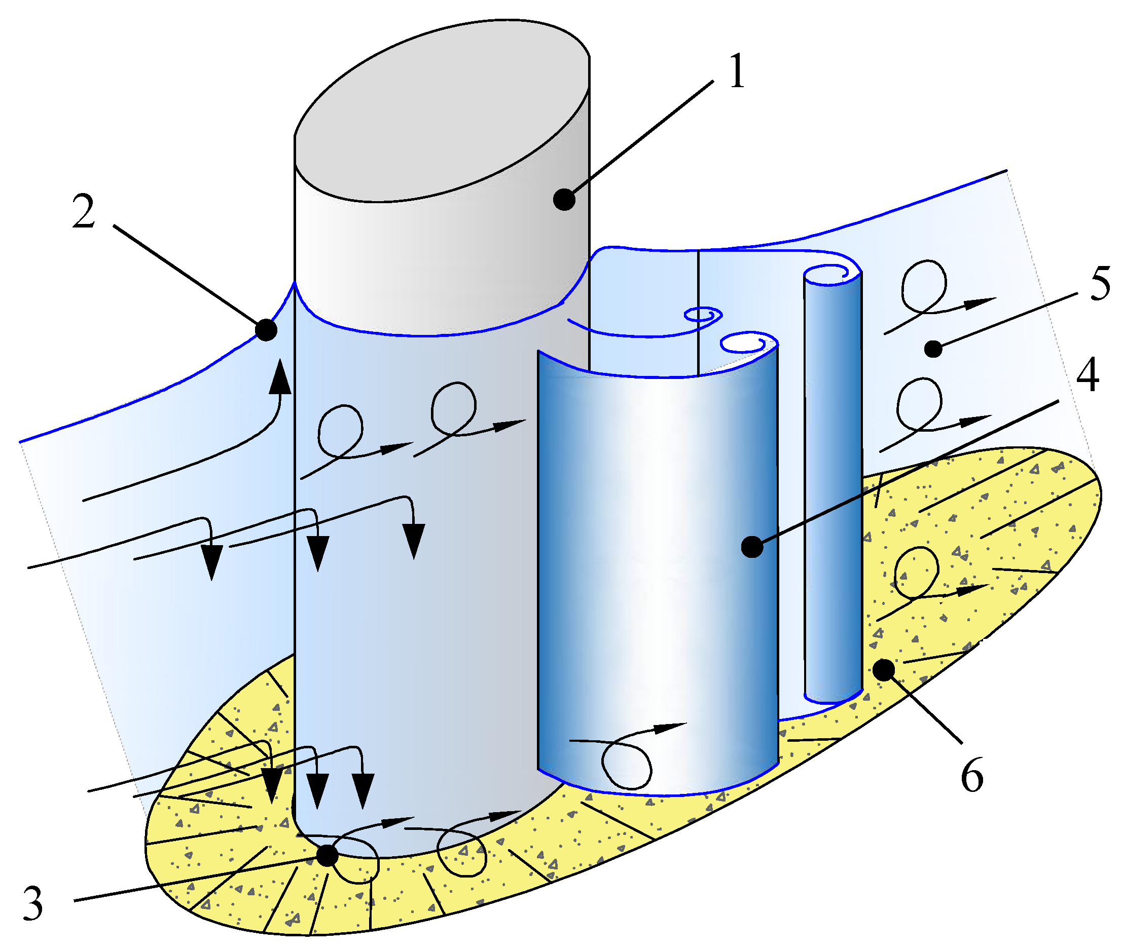
When the stream flows through the bridge section, the water level is piled up upstream the crossing. On the inflow side, in front of the pillar face, the subsurface stream flows upwards towards the free water surface, and the bottom stream heads towards the bottom (Figure 1). Simultaneously, the water masses flow down the pier (1 in Figure 1). These two mutually interacting phenomena cause the form of water movement to gain the features of three-dimensional turbulent flow. The masses of water directed upwards create a frontal wave in front of the pillar (2 in Figure 1). The stream hitting the bottom creates a horseshoe vortex (3 in Figure 1) [2,14]. From the upstream cross-section of the contracted stream, initial vortices are formed at its depth, which, as they flow around the pier, take the form of a lee-wake vortex (4 in Figure 1). Vertical vortices moving around the pier downstream create a run-off whirlpool zone with farwater vortices occurring downstream the bridge section (5 in Figure 1). The vortices’ intensity decreases rapidly as they diverge from the pier, which causes the sediment settling on the outflow side, especially in the case of long piers [4,15].
To initiate sediment transport, the water velocity, named non-washable velocity, is needed. Below this velocity, the sediment is not exposed to displacement, and after exceeding this velocity, the movement of grains begins. However, in laboratory practice, it is impossible to measure water flow velocity at the bottom in the zone of direct stream influence on the soil particles. Therefore, a vertical or cross-sectional velocity distribution is assumed.
According to Melville and Chiew [16], a horseshoe vortex increases the flow velocity in the bottom area by flowing down the river while lifting whirls carry the eroded material downstream. When the soil loss is greater than the amount of incoming sediment in the pier’s area, the stream’s bottom washes out to form a scour hole. The increasing depth of the scour hole is accompanied by a decrease of horseshoe vortices, which reduces the ability to lift the soil from the pier’s vicinity. Under live-bed conditions, when the hole is filled with the sediment transported from the upstream, there is a balance between removing and delivering the soil and then, the process of forming the scour hole impounds. Under clear-water conditions, when the shear stress on the bed, caused by horseshoe vortices, becomes less than the critical shear stress, the scour hole stabilizes its dimensions [2,4].
2. Materials and Methods
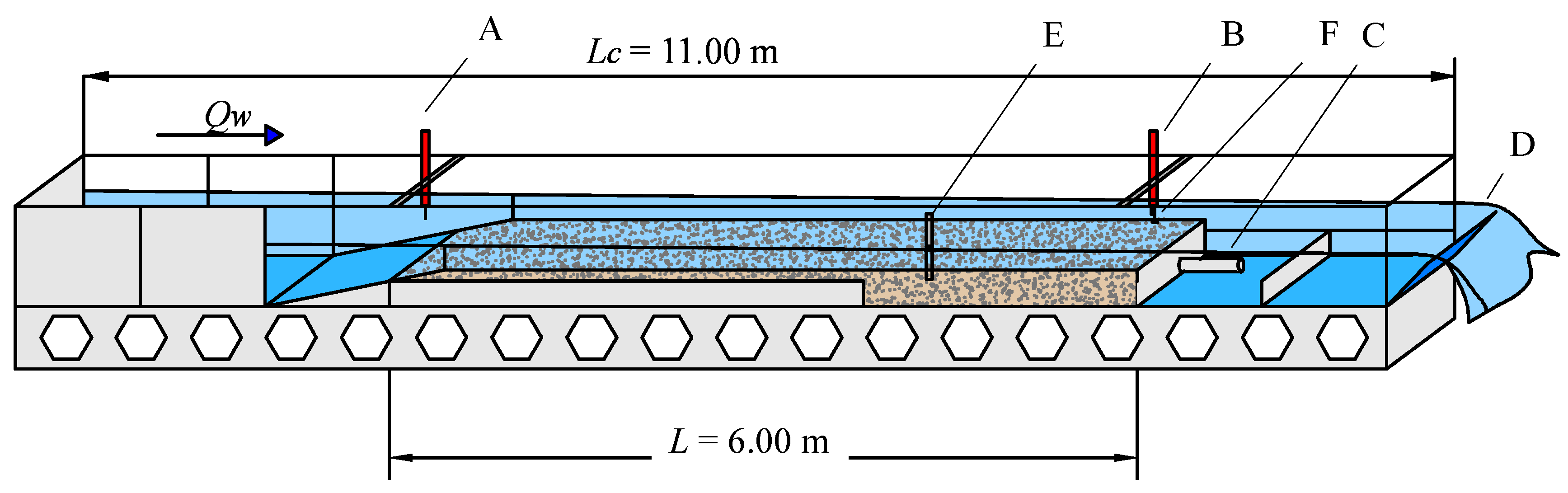
The research was carried out on a physical model with a sandy bottom in a rectangular flume with a total length Lc = 11.00 m and width W = 0.58 m (Figure 2 and Figure 3).
A movable pin water level gauge (B in Figure 2) was used to measure the level of water surface and was moved along the test flume. The water surface level was regulated by a gate (D in Figure 2) located at the end of the laboratory flume. The sandy bottom shape was measured with a moving sound probe (B in Figure 2) integrated with a movable pin gauge, traversed along and across the flume. A closed water circulation system is used in the laboratory. This system’s main element is an underground reservoir, from which water is piped by a lift-and-force pump to the upper equalizing tank.
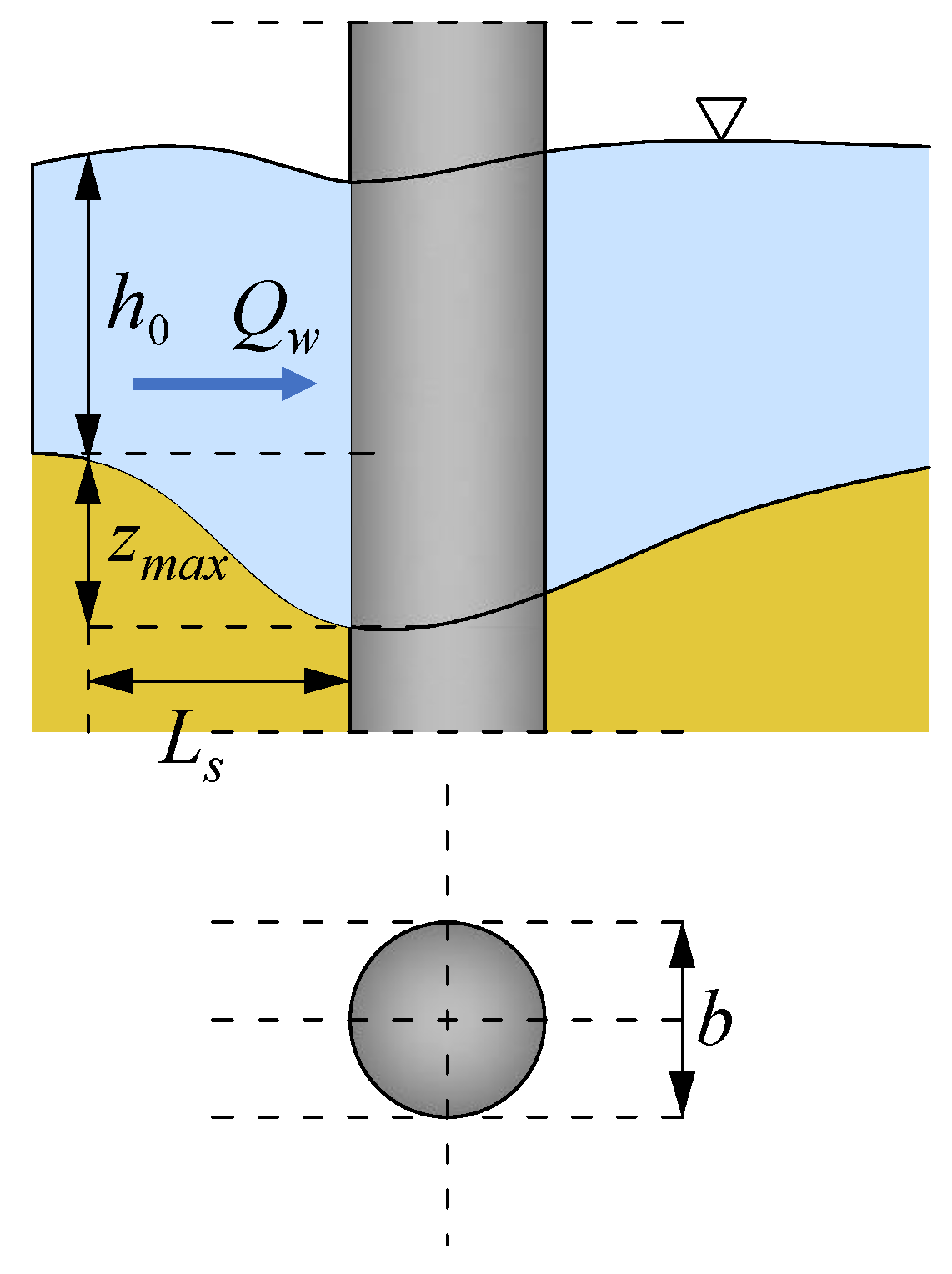
Measurements were taken under the sediment transport maintenance conditions: sediment transport was ensured by providing hydraulic conditions that cause a bed shear exceeding the critical stress. Then grains were lifted by the water stream and moved downstream by the flowing water to the pier’s area. The bottom material was coarse, uniform, well-sorted sand with characteristic diameters d50 = 0.91 mm and d90 = 0.99 mm. The density index ID was equal to 0.77–0.82, i.e., the soil was compacted. Before each measurement, the sand after leveling the bottom surface was compacted with a 3.5 kg hand compactor, lowered to the bottom surface with an energy of about 5 J. The local scour scheme and characteristic geometry properties measured near the pier model during research are shown in Figure 4. The maximum depth of the scour hole zmax and its total length Ls was measured upstream the pier.
Laboratory tests were carried out under steady flow conditions, in the range of Qw = 0.020–0.043 m3 s−1 and water depth established before scouring h0 = 0.07–0.15 m, was measured in the distance of 50 cm upstream the pier. Table 1 displays the main parameters of 19 test series.
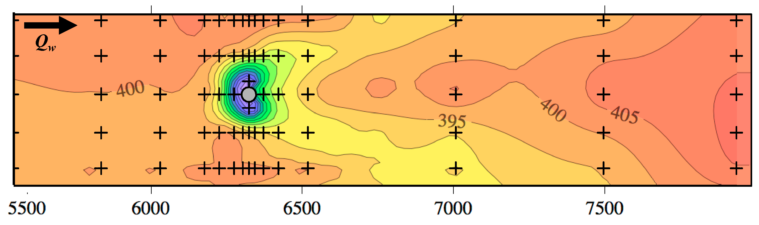
Measurements of the bed shape at selected points were made using sound probe. The probe readings were recorded by the researcher providing data in the form of points with (x, y, z) coordinates, where x is flume width, y is flume length and z is the bed level. The initial studies on the bed shape were carried out before the water flow was introduced into the model, then the bed shape measurements were performed in established time steps (1–2 h). The final shape of the bottom was read after 7.5–10 h of measurement, directly after draining the water from the model. The arrangement of measurement points on the test section surface of the flume is shown in Figure 5, where the local scour shape measured in a case of test series No. 14, characterized by Qw = 0.036 m3 s−1 and h0 = 0.10 m is presented. The symmetry of the resulting scour hole with respect to the longitudinal axis of the flume can be observed. The length of the scour upstream is greater than the progressive scour downstream of the pier. The accumulation of sediment in the pier axis from the outflow side in the farwater vortex area is also visible (see also Figure 6). In these particular hydraulic conditions, with water depth-to-width of pier ratio h0/b = 0.172 experimental pier type could be considered as wide.
Selected empirical formulas used to estimate the local scour’s maximum depth in the ridge pier area were verified. The formulas were chosen on the basis of their applicability ranges. The article compares the results of its own measurements of the scour’s hole depth in the vicinity of a single pier with depths calculated by the use of Begam’s formula [5], a formula included in the Regulation of the Polish Minister of Transport and Maritime Economy of 30 May 2000 on technical conditions to be met by road engineering structures and their location [11] and Laursen and Toch formula [12].
2.1. Begam Formula
Begam’s formula takes into account the granulometric parameters of the sediment, represented by non-washable velocity vn (the velocity not causing the intensive sediment transport according to Dąbkowski et al. [5]), hydraulic characteristic w, dimensions and position of a pier or piers in relation to the stream, described by coefficients α, β, M and K. The general form of Begam’s formula is follows:
where:
—correction coefficient including the size of the examined hydraulic, for laboratory experiments ;
—the constant value of the regression equation determined by Begam for laboratory tests, describing the water depth h0 magnitude, = 7.83;
—coefficient, dependent on the pier width-to-water depth in the direct vicinity of a pier before scouring (b/h0), calculated as following:
b—pier width, m;
h0—water depth in the direct vicinity of a pier before the scouring (m);
k—the constant value of the regression equation determined by Begam for laboratory tests, describing pier width b magnitude, k = 0.0177;
v—incoming stream velocity (m s−1);
vn—non-washable velocity, for non-cohesive soils calculated according to Studeničnikow (m s−1) after Dąbkowski et al. [5]:
—particle fall velocity of medium size grains (m·s−1), calculated according to Gončarov [5] the grain size range of 0.15 mm < d < 1.5 mm, including medium water temperature during measurement t and the specific weight of sediment and water (N m−3):
M—coefficient depending on pier shape and construction, for a single cylindrical pier M = 1.0;
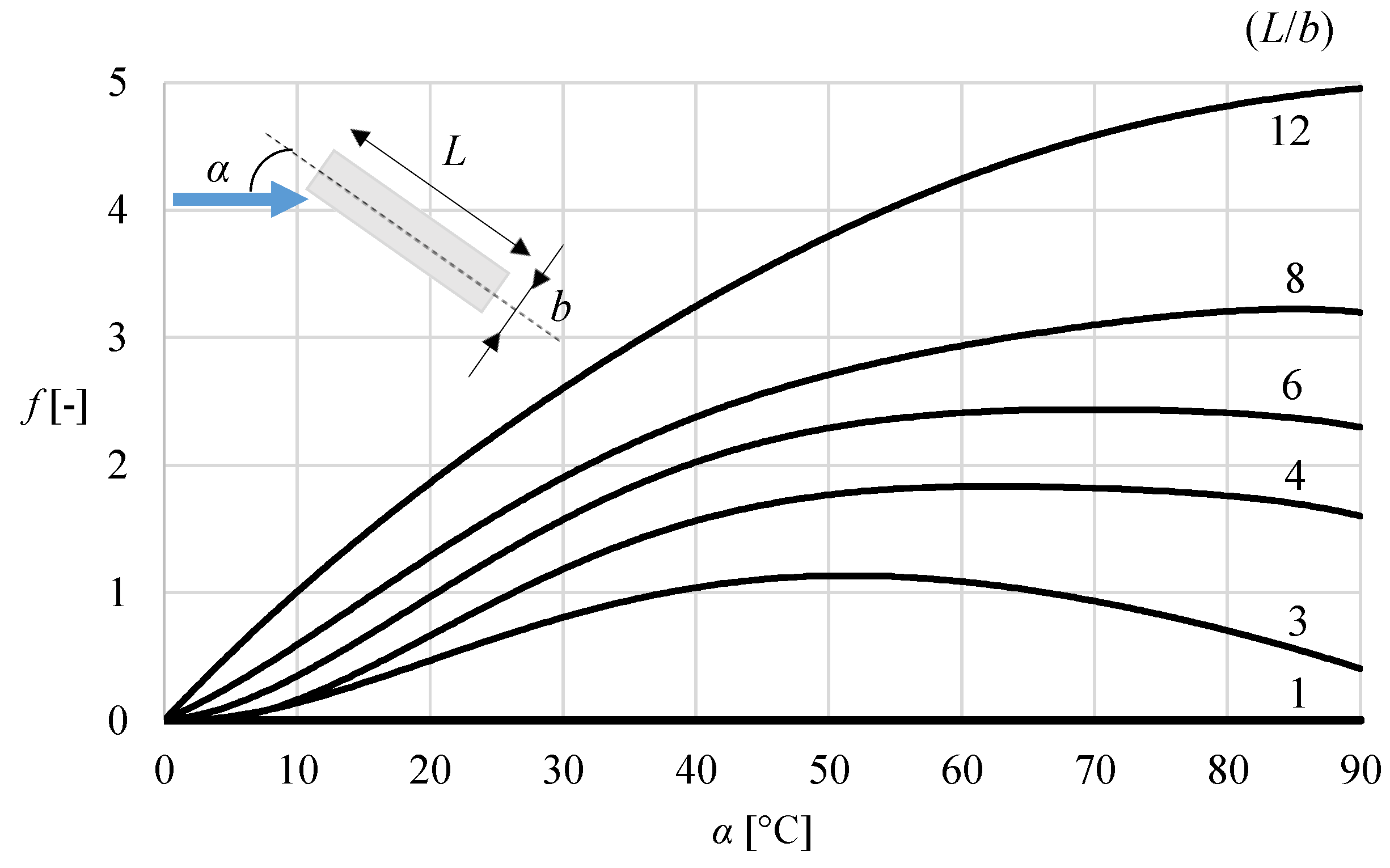
K—coefficient depending on pier dimensions and the angle between pier longitudinal axis and the main stream direction, calculated as:
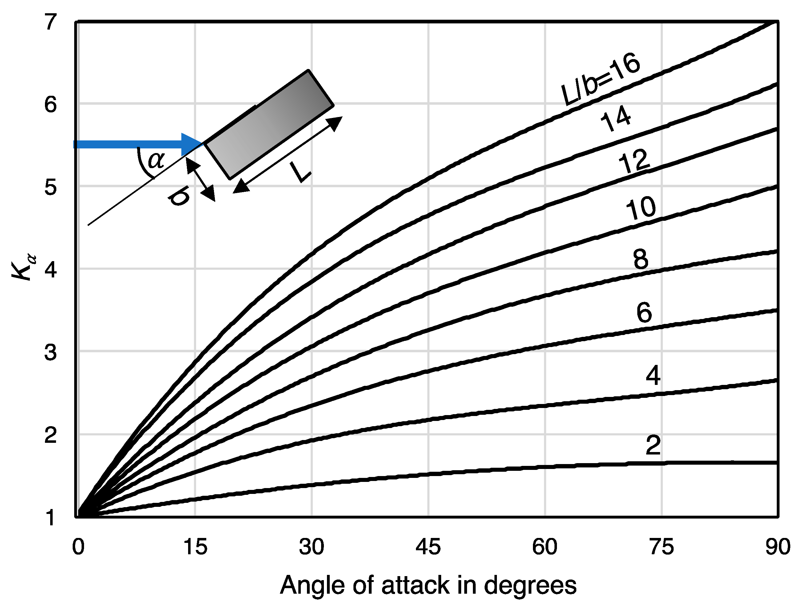
where f is the coefficient dependent on an angle α between the pier longitudinal axis and the main stream direction and the pier length-to-width (L/b) ratio. The values of f coefficient can be read from the nomogram included in the Figure 7. For α < 10° K = 1.0 can be assumed [5]. Calculated parameters of the Equation (1) are in Table 2.
2.2. The Regulation of the Polish Minister of Transport and Maritime Economy Formula
The Regulation contains a formula for calculating the maximum depth of local scour underneath a bridge, referring it to the shape of a pier, stream velocity upstream the bridge, type of soil and the direction of water inflow to the pier:
where:
K1—coefficient dependent on the pier shape, in the present case of a single cylindrical pier K1 = 10.0; K1 coefficient values for most common pier shapes are given in Table 3.
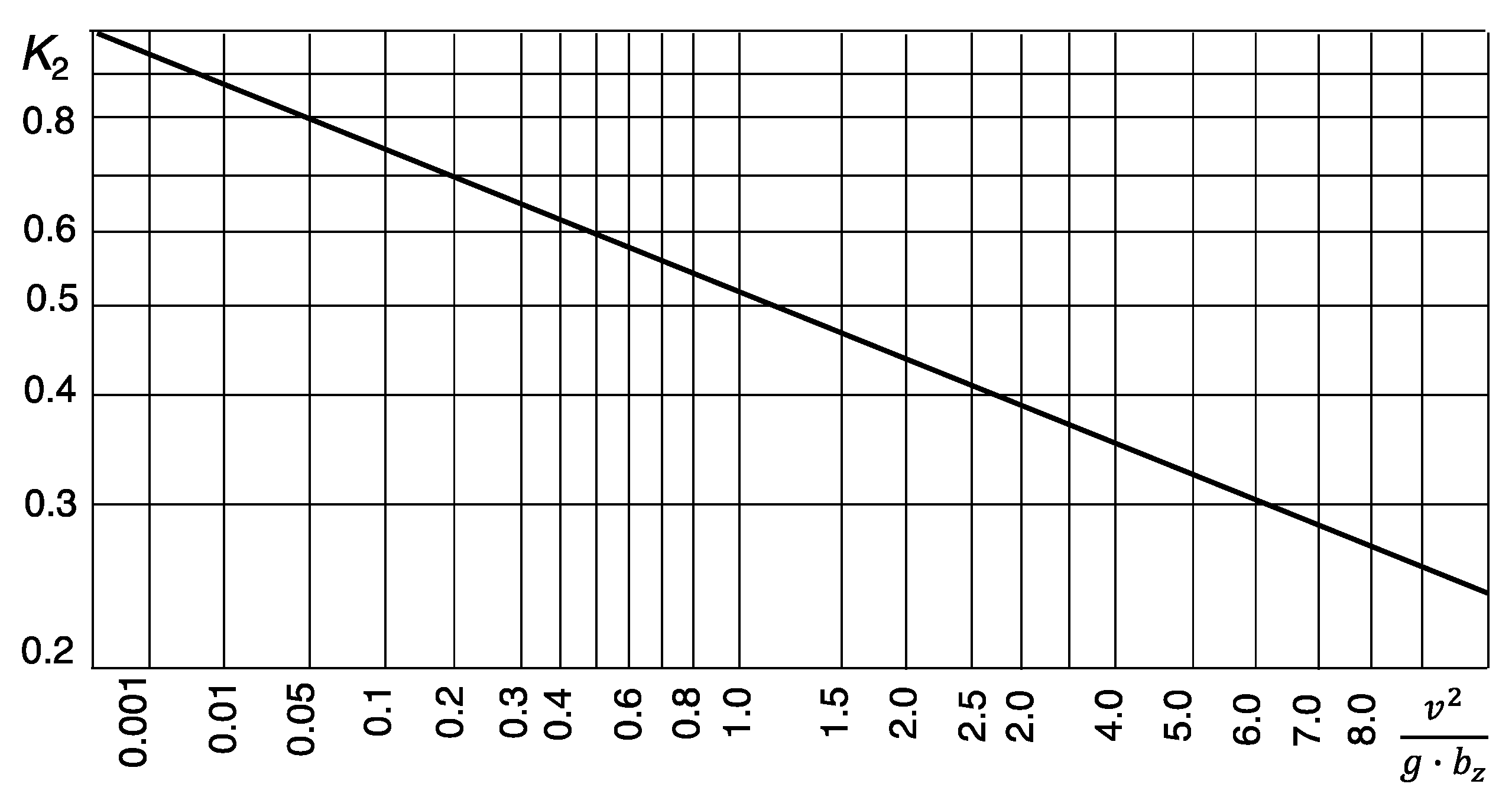
K2—coefficient being the function of equivalent pier width bz in a form of v2/gbz, presumed as:
- for A, B and D pier shape types, with bz = b;
- for A, B and D pier shape types, with bz = L sin + b cos;
- for C pier shape types, with any bz = b.
where is the angle of the axis of the pier with the direction of the flow, L is a pier length or a group of piers’ length. For the present case of single cylindrical pier with C shape type, the equivalent pier width bz is equal to the actual pier width b. K2 parameter values for any test series were read from the Figure 8.
a—coefficient including the velocity distribution in a cross-section field, for the main riverbed a = 0.6 (-),
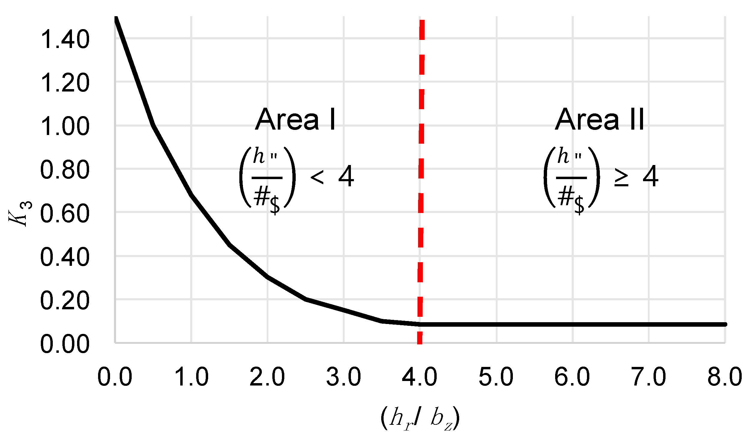
K3—coefficient depending on the ratio of the water depth over the scour hole to equivalent pier width hr/bz (-). The magnitude of bottom lowering due to local erosion is expressed by the degree of scouring of bridge section P. P is the ratio of the average water depth over eroded riverbed hr and before the scour formation h0. Permissible values of the degree of a scouring, depending on the method of support foundations, are given in Table 4.
The analyzed model of a cylindrical pier was classified as a support with a semi-streamlined foundation shape within the scour boundaries, founded directly in the ground, therefore P = 1.0 and hr = h0 (row 4 in Table 4).
To determine K3 Figure 9 was used, depicted in accordance with the Regulation of Polish Minister (Journal of Laws of 2000 No. 63, item 735). The following function described the curve:
which allows for the calculation of parameter K3 = f (hr/bz) without requiring each time the values from the charts to be read. The results of the readings are summarized in Table 5.
c—coefficient depending on bedload soil granulation. For loose soil can be applied. In researched laboratory conditions for d90 = 0.0099 m, c = 0.297 m. Computational parameters of the Equation (6) are shown in Table 5.
In river valleys with an insignificant bed inclination within the watercourse, where water stream turbulence is reduced, the zmax value calculated according to Equation (6) must be decreased by 20%. Therefore, for the research flume, the final value of the local scour was determined as 0.80 of the value calculated according to the Equation (6). Considering constant values, the final Equation (6) for the conditions prevailing on the tested model of the bridge pier has the form:
2.3. Laursen & Toch Formula
The formula developed by Laursen and Toch [12] has been used to estimate the forecasted scour hole dimensions on all intermediate bridge pillars since the early 1970s. Despite its simplicity, it has gained great popularity and acceptance among engineering communities in the United States. It is used for piers founded in riverbeds with a uniform bedload. The general form of the equation is as follows:
where:
—coefficient depending on the shape of a pier. The value of this coefficient for different pier shapes is given in Table 6. For the analyzed case of a cylindrical pier, the value of coefficient = 0.9.
—coefficient depending on the orientation of the longitudinal axis of a pier in relation to main stream direction, selected from the diagram in Figure 10. Its value for conditions occurring in laboratory tests was = 1.0.
2.4. Monte Carlo Sampling Method Application
The analyses were based on the formulas given in individual sources. Formulas optimized by authors also include parameters given in each source formulas. Using the Monte Carlo method [17], the authors verified only constant coefficients of the equations. For individual formulas, these were: th and k of the Equation (1) describing Begam equation and m and n describing the Equation (9) developed by Laursen & Toch [12]. Equation (8) according to the Regulation of the Polish Minister of Transport and Marine Economy of 30 May 2000 [11] does not contain constant coefficients; therefore, a correction factor K0 was introduced to consider the laboratory testing conditions.
The measure of coefficients’ value adjustment to laboratory results was the average relative error δ for all 19 measurement series as a ratio of the absolute error of an estimation to the measurement being taken—the smaller the function, the more accurately it describes the results of laboratory tests. The aim of the applied procedure was to obtain optimized forms of equations describing the results of laboratory measurements. The dimensionless parameters of the function were generated within the accepted ranges of values by Monte Carlo method application, involving multiple sampling of random numbers and calculation of the average error for all test series, using the equation described by a given set of parameters. The analyses were carried out under the following assumptions:
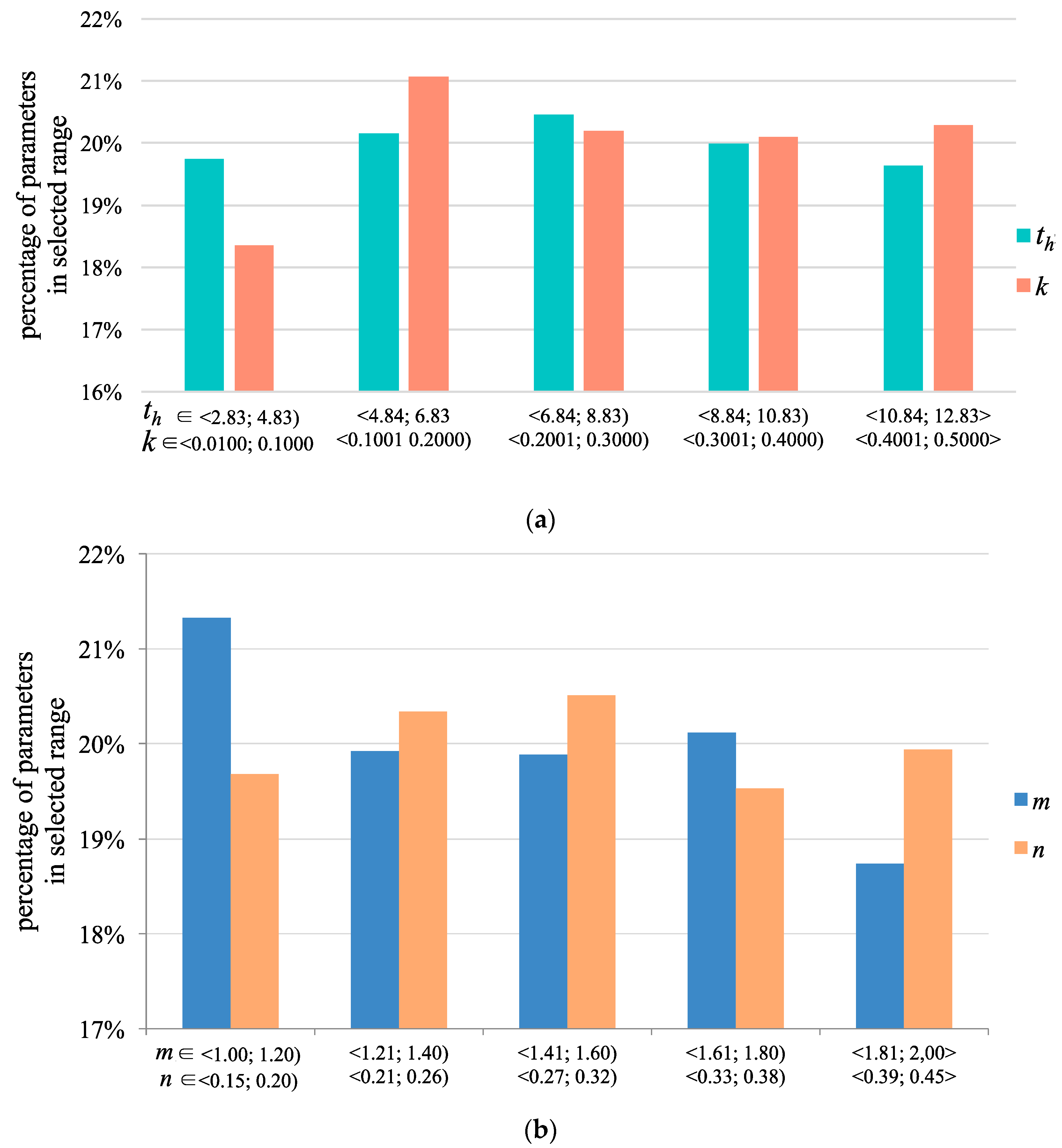
- for Begam’s formula [5] 10,000 combinations of parameters describing the Equation (1) were randomized, i.e., the function coefficient th describing the water depth h0 magnitude (in the original form of the formula this coefficient is equal to 7.83) and the function coefficient k, describing the pier width b magnitude (in the original form of equation coefficient k = 0.0177). The parameter th was range 1.30 ± 33% and the exponent of n function in the range 0.30 ± 50%. The results are listed in Table 7 and their geometric interpretation is shown in Figure 12b.
3. Results
For the original form of Begam’s equations (Equation (1)), the Regulation’s equation (Equation (8)) and Laursen’s and Toch’s equations (Equation (9)), average relative errors δ are obtained:
- δ = 21.6% for Begam function described with th and k parameters proposed with the original form of equation; th = 7.83; k = 0.0177.
- δ = 30.1% for the formula included within Regulation of the Polish Minister of Transport and Marine Economy of 30 May 2000 with coefficient K0 proposed in the original form of equation; K0 = 1.00.
- δ = 15.3% for Laursen and Tochand Toch function described with m, n parameters proposed with the original form of equation; m = 1.5; n = 0.3.
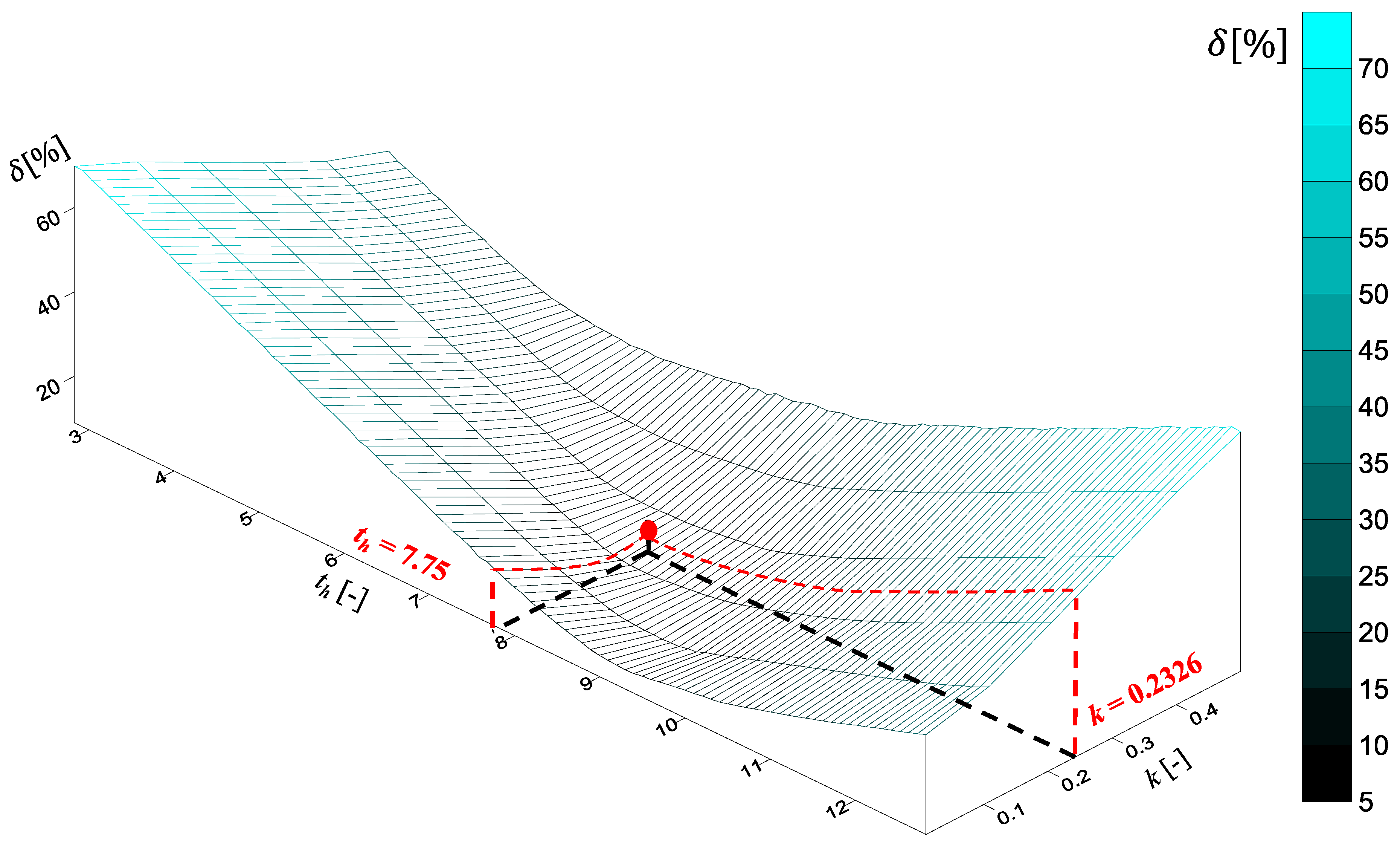
In the case of Begam’s formula, the results of the Monte Carlo sampling analysis showed the best fit to the laboratory data using the specific parameters of the adopted Equation (1) of th = 7.75 and k = 0.2326. The derived formula can be presented in the following way:
The average relative error for the whole set of 19 test series was 8.8%. The variability of the magnitude of medium relative errors δ was between 8.8 and 69.9% for the group of parameters in the tested range th ∈ <2.83; 12.83> and k ∈ <0.01; 0.50>. The variability of the parameters of Equation (1) in the analysis of matching to laboratory data is shown graphically in Figure 13. The kriging geostatic interpolation method [18,19] was used to present graphical results.
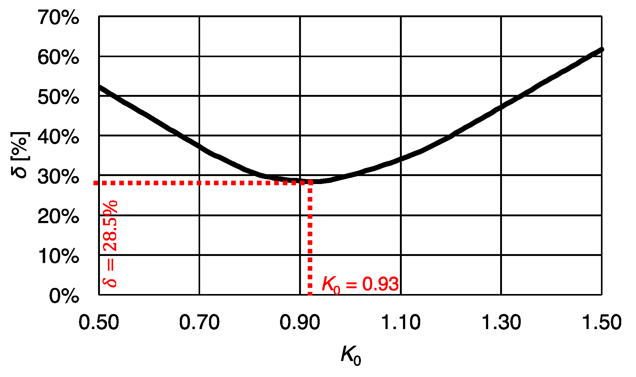
In case of the formula included in the Regulation of the Polish Minister of Transport and Marine Economy of 30 May 2000 (Journal of Laws 2000 No 63, item 735), to which a correction factor considering laboratory testing conditions K0 was introduced, the best fit of the formula to the laboratory results was obtained at K0 = 0.93. Thus, the form of the formula, based on Begam equation, adapted to the laboratory data takes the form:
Within the assumed range of K0 ∈ <0.50; 1.50> a spread of average relative errors was achieved in the range of 28.5–61.7% (Figure 14).
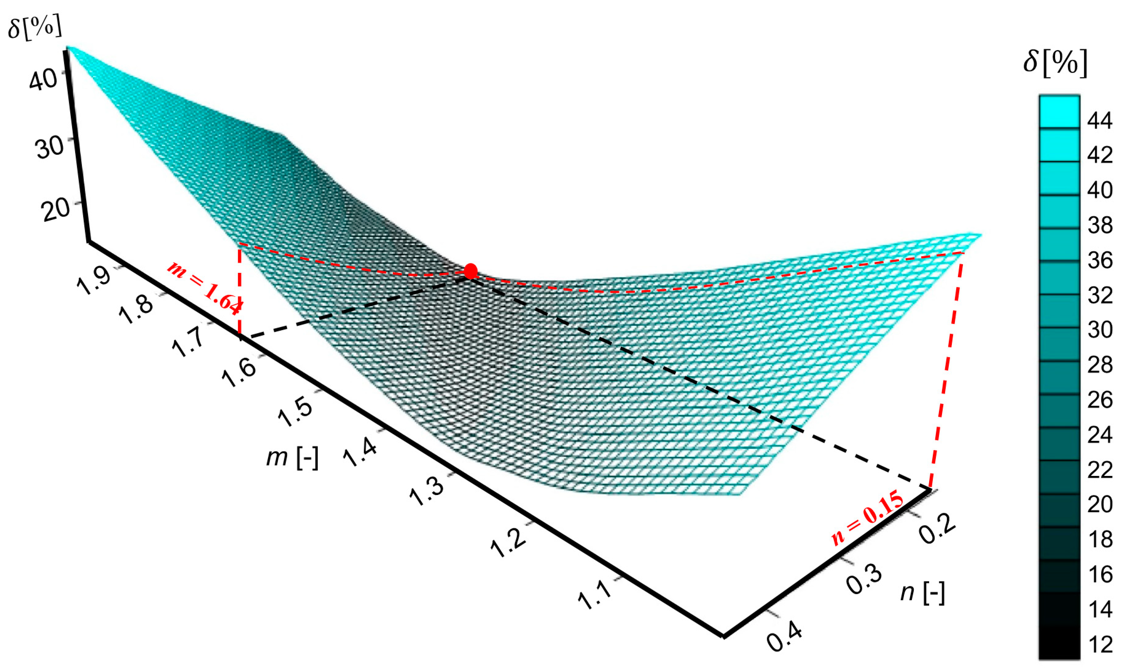
For Laursen and Toch formula, the best fit, measured by the smallest mean relative error δ, for all 19 test series, was obtained for parameters m and n equal to 1.64 and 0.15, respectively, whereas the parameters originally proposed as a function are m = 1.50, n = 0.30. The mean relative error δ for all series of measurements is 13.8%.
The research of function fit to data variability depending on the adopted parameters m and n is shown in Figure 15. For the parameters of the function sampled in the range under consideration, errors in the range 13.8% to 43.6% were obtained. Based on the results of the analysis it is proposed to modify Laursen and Toch formula for the present laboratory conditions, replacing the original values of parameters m = 1.50 and n = 0.30 with values calculated m = 1.64; n = 0.15:
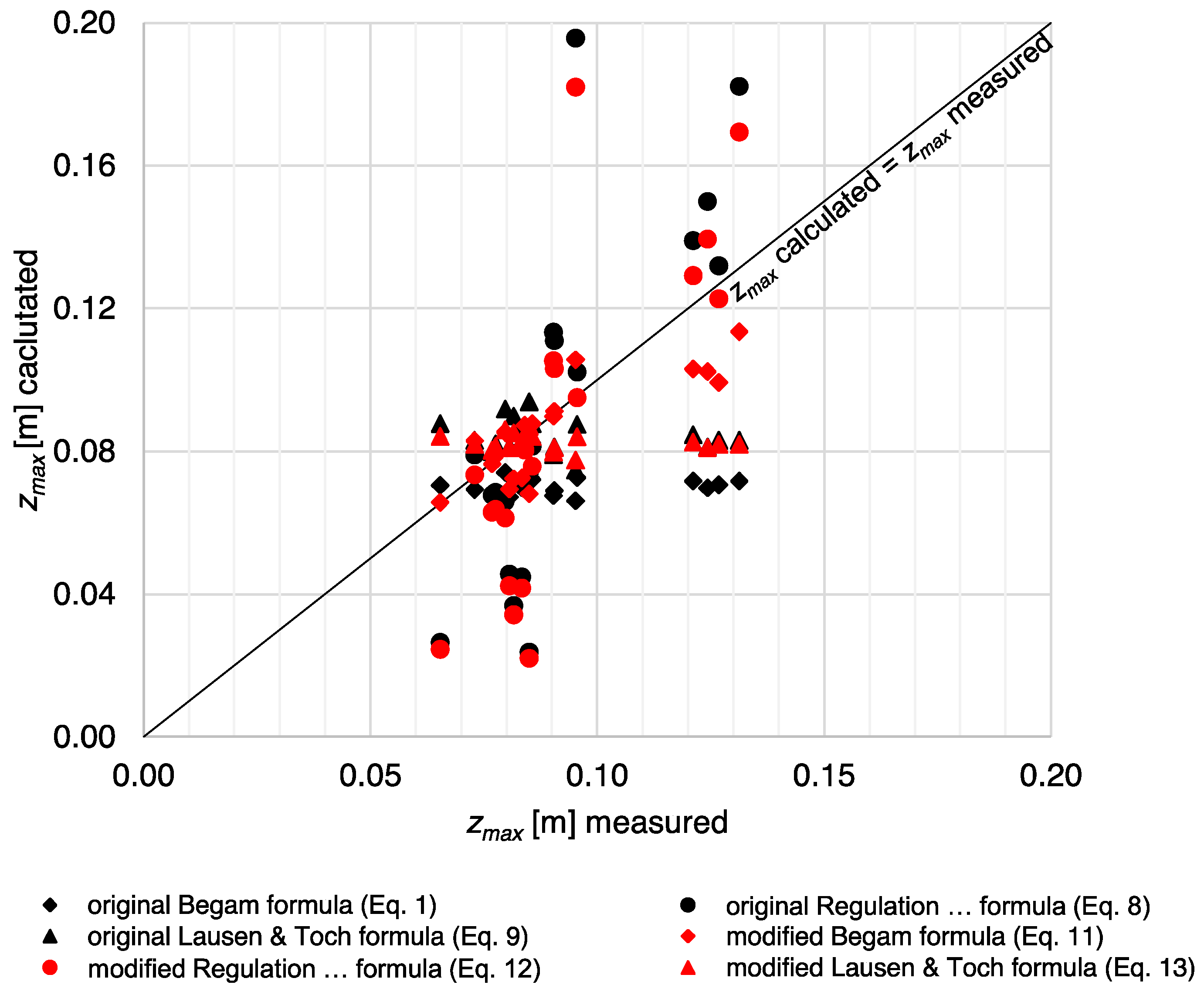
The results of the verification of the formulas described are presented in Table 8 and illustrated graphically in Figure 16. Table 8 shows the mean square error of the MSE, and the mean relative error of each of the δ formulas tested, as well as the mean measurement uncertainty uc(y) of each of the formulas tested. Determining the measurement uncertainty is a necessary part of every measurement procedure and the components of the proposed empirical models are classified as uncorrelated indirect measurements. Taking into account the accuracy of the measurement of each of the elements measured directly during laboratory testing, the complex standard uncertainty of each uc(y) equation was calculated using the formula:
where K is the number of quantities measured directly, symbols x1, x2, x3, …, , means k of directly measured quantities, and u(x1), u(x2), u(x3), …, u() are their standard uncertainties. The standard uncertainties of directly measured quantities can be calculated in two ways:
- where the values show no dispersion or where only one measurement result is available:where n—observation number, —the numerical value of the expected value estimator or:
- when several measurement results are available:where is 10 the units of the decimal place with the lowest value.
4. Conclusions
As part of the laboratory tests, 19 series of flume bed shape and water surface elevation measurements with a duration of 7–10.5 h were carried out to investigate the local scour evolution under given hydraulic conditions. In the area of the bridge pier model in the hydraulic flume, the bottom was locally eroded and a local erosion took place. Its geometrical dimensions and position were determined using a disc probe. The maximum scour hole depth was also calculated using three empirical formulas, taking into account hydraulic, granulometric and geometric parameters of the testing stand, pier shapes and dimensions.
The analyses included Begam’s formula given by Dąbkowski et al. [5], the equation proposed by the Regulation of the Polish Minister of Transport and Marine Economy [11] and Laursen and Toch formula [12]. The comparison of the calculated and directly measured local scour depths in the laboratory indicated that the laboratory test results are best described by Laursen and Toch’s formula (Equation (12)) with an average relative error of 15.3%, despite its simplicity and a small number of considered parameters describing the river bed and bridge development geometry properties, bridge crossing and sediment granulation. Begam’s formula (Equation (1)) provides an adjustment of calculated values to the measured with a medium relative error of 21.6%. The adjustment for Regulation of the Polish Minister of Transport and Marine Economy (Equation (8)) according to the medium relative error of measurement and calculation results was 30.1%.
The Monte Carlo sampling method allowed us to optimize the original formulas to calculate the scour’s depth near the bridge piers. In optimizing the parameters, the criterion of minimizing the relative error of matching the formula to the data was used. In the case of the Begam formula (Equation (11)), optimization allowed to reduce the medium relative error by 12.8%; in the case of the formula from Regulation of the Polish Minister of Transport and Marine Economy (Equation (12)), this reduction was 1.6%, and for Laursen and Toch formula (Equation (13)) by 1.5%. Differentiation of laboratory test conditions of each of the 19 test series resulted from hydraulic conditions, i.e., discharge and water depth. Therefore, water stream velocity determines the conditions of sediment transport. The analyses were carried out on the same construction of the test stand and granulometric conditions of the bottom. For other test conditions, the necessity to verify the obtained Equations (11)–(13) should be performed. Adaptation of the presented or other formulas can be carried out using the Monte Carlo method as presented in this paper.
Author Contributions
Conceptualization, M.K. and S.B.; Methodology, M.K.; Validation, M.K.; Formal analysis, M.K., J.U. and S.B.; Investigation, M.K.; J.U.; Writing—original draft preparation, M.K.; Writing—review and editing, M.K., J.U. and S.B.; Visualization, M.K.; Supervision, S.B.; Funding acquisition, J.U. All authors have read and agreed to the published version of the manuscript.
Funding
This research received no external funding.
Conflicts of Interest
The authors declare no conflict of interest.
References
- Bajkowski, S. Wpływ mostu Siekierka na warunki przepływu wezbrań na rzece Zwoleńka. Wiadomości Melioracyjne i Łąkarskie 2015, 58, 23–29. (In Polish) [Google Scholar]
- Graf, W.H. Fluvial Hydraulics: Flow and Transport Processes in Channels Of Simple Geometry; John Wiley & Sons: Chichester, UK, 1998. [Google Scholar]
- Esmaeili, T.; Dehghani, A.A.; Zahiri, A.R.; Suzuki, K. 3D Numerical simulation of scouring around bridge piers (Case Study: Bridge 524 crosses the Tanana River). World Acad. Sci. Eng. Technol. 2009, 58, 1028–1032. [Google Scholar]
- Jarominiak, A. Zabezpieczenie przed rozmyciem dna cieków przy filarach mostów. Drogownictwo 2016, 10, 303–312. (In Polish) [Google Scholar]
- Dąbkowski, L.; Skibiński, J.; Żbikowski, A. Hydrauliczne Podstawy Projektów O Wodnomelioracyjnych; PWRiL: Warszawa, Poland, 1982. (In Polish) [Google Scholar]
- Tymiński, T. Hydrauliczne badania modelowe filarów mostowych na przykładzie wybranych mostów Opola. Rocznik Ochrona Środowiska 2010, 12, 879–893. (In Polish) [Google Scholar]
- Sturm, T.W. Enhanced Abutment Scour Studies for Compound Channels; Federal Highway Administration: McLean, Virginia, 2004.
- Chandara, M.; Genguang, Z.; Vouchleang, H.; Shuang, Z.; Yulin, F. Assessment of turbulence models on bridge-pier scour using Flow-3D. World J. Eng. Technol. 2019, 7, 241–255. [Google Scholar]
- Lee, F.; Lai, J.; Lin, Y.; Chang, K.; Liu, X.; Huang, C. Prediction of bridge pier scour depth and field scour depth monitoring. In Proceedings of the River Flow 2018-Ninth International Conference on Fluvial Hydraulics, Lyon-Villeurbanne, France, 5–8 September 2018; p. 03007. [Google Scholar]
- Breusers, H.N.C.; Nicollet, G.; Shen, H.W. Local scour around cylindrical piers. J. Hydraul. Res. 1977, 15, 211–252. [Google Scholar] [CrossRef]
- Regulation of the Minister of Transport and Maritime Economy of 30 May 2000 on technical Conditions to be Met by Road Engineering Structures and Their Location; Journal of Laws 2000 No. 63, item 735; Ministry of Transport, Construction and Maritime Economy: Warsaw, Poland, 2000.
- Laursen, E.M.; Toch, A. Scour around Piers and Abutments; Iowa Institute of Hydraulic Research: Iowa City, IA, USA, 1956. [Google Scholar]
- Copp, H.D.; Johnson, J.P.; McIntosh, J.L. Prediction methods for local scour at intermediate bridge piers. Transp. Res. Res. 1988, 1201, 46–53. [Google Scholar]
- Chavan, R.; Gualtieri, P.; Kumar, B. Turbulent flow structures and scour hole characteristics around circular bridge piers over non-uniform sand bed channels with downward seepage. Water 2019, 11, 1580. [Google Scholar] [CrossRef] [Green Version]
- Van Rijn, L. Local Scour Near Structures. Available online: https://www.leovanrijn-sediment.com (accessed on 13 November 2019).
- Chiew, Y.M.; Melville, B.W. Local scour around bridge piers. J. Hydraul. Res. 1987, 25, 15–26. [Google Scholar] [CrossRef]
- Niederreiter, H. Random Number Generation and Quasi-Monte Carlo Methods; Society for Industrial and Applied Mathematics: Philadelphia, PA, USA, 1992. [Google Scholar]
- Davis, J.C. Clarification. In Statistics and Data Analysis in Geology, 3rd ed.; John Wiley & Sons: New York, NY, USA, 1986. [Google Scholar]
- Goldsztejn, P.; Skrzypek, G. Applications of numeric interpolation methods to the geological surface mapping using irregularly spaced data. Przeglad Geol. 2004, 52, 233–236. [Google Scholar]
Figure 1.
Flow pattern and local scour around a cylindrical pier schematic: 1—pier, 2—frontal wave, 3—horseshoe vortex, 4—lee-wake vortex, 5—farwater vortex, 6—local scouring area.
Figure 1.
Flow pattern and local scour around a cylindrical pier schematic: 1—pier, 2—frontal wave, 3—horseshoe vortex, 4—lee-wake vortex, 5—farwater vortex, 6—local scouring area.

Figure 2.
Test flume construction (dimensions in meters), where: Qw – water discharge; A—pin water gauge; B—sound probe equipped with movable pin gauge (F); C—collection chamber with the drainage; D—regulatory gate; E—pier; Lc —total flume length; L—sandy bed length.
Figure 2.
Test flume construction (dimensions in meters), where: Qw – water discharge; A—pin water gauge; B—sound probe equipped with movable pin gauge (F); C—collection chamber with the drainage; D—regulatory gate; E—pier; Lc —total flume length; L—sandy bed length.

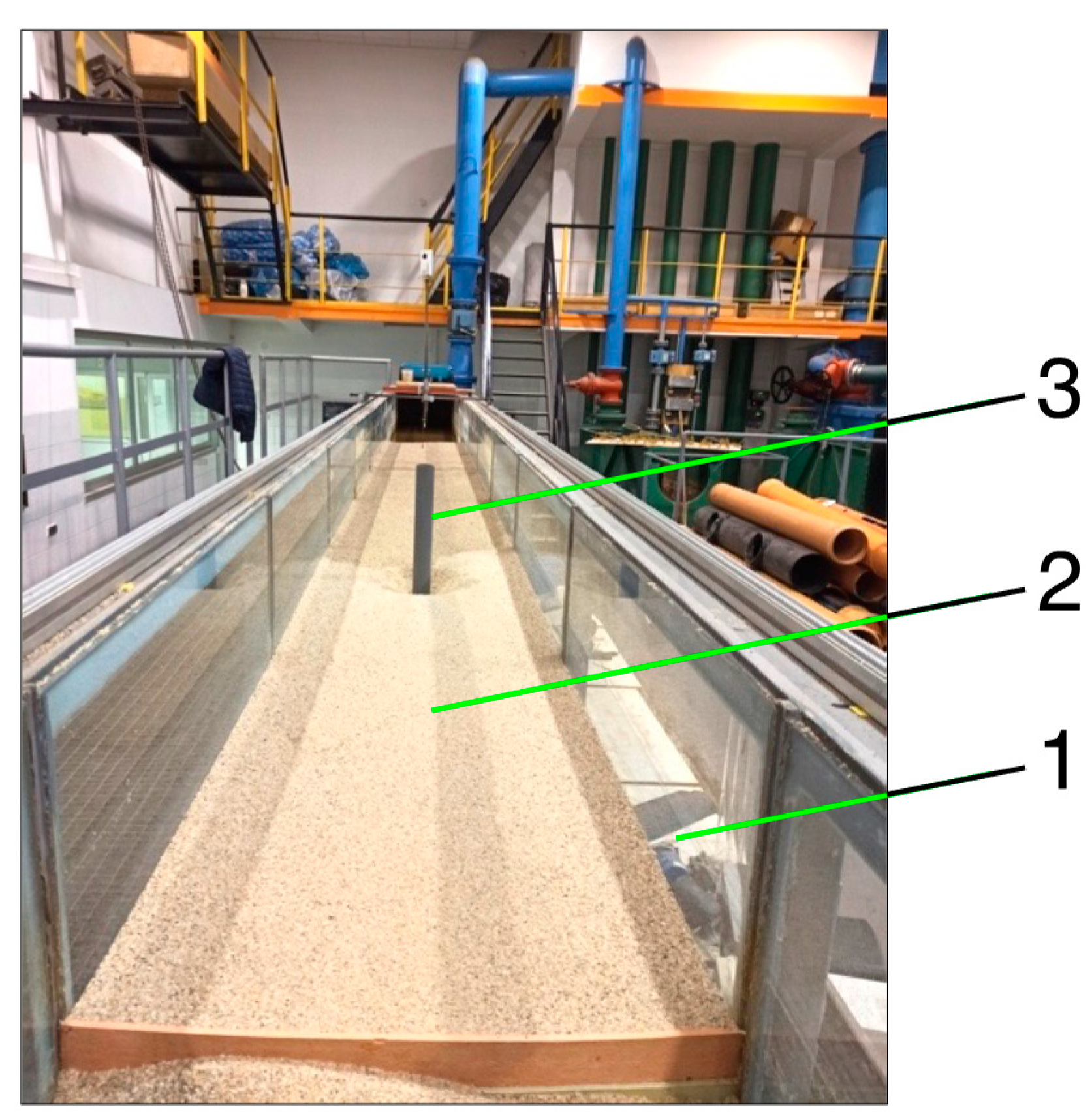
Figure 3.
Laboratory flume—view from downstream: 1—tilting glass flume, 2—erodible bed, 3—bridge pier model.
Figure 3.
Laboratory flume—view from downstream: 1—tilting glass flume, 2—erodible bed, 3—bridge pier model.

Figure 4.
Pier model and scour parameters: h0—water depth, zmax—maximal scour depth, Qw—water discharge, b—pier diameter, Ls—upstream scour length.
Figure 4.
Pier model and scour parameters: h0—water depth, zmax—maximal scour depth, Qw—water discharge, b—pier diameter, Ls—upstream scour length.

Figure 5.
Measuring grid and 2D contour plan of scour for laboratory data for Qw = 0.036 m3 s−1, h0 = 0.10 m (basing on own laboratory data).
Figure 5.
Measuring grid and 2D contour plan of scour for laboratory data for Qw = 0.036 m3 s−1, h0 = 0.10 m (basing on own laboratory data).

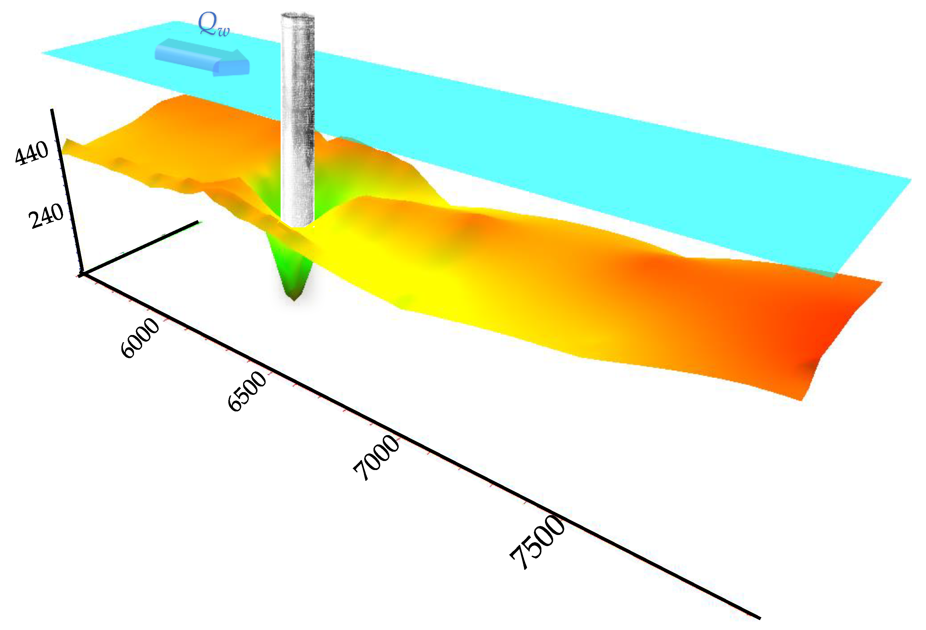
Figure 6.
Local scour and pier model shape for Qw = 0.036 m3 s−1, h0 = 0.10 m (basing on own laboratory data).
Figure 6.
Local scour and pier model shape for Qw = 0.036 m3 s−1, h0 = 0.10 m (basing on own laboratory data).

Figure 7.
Coefficient f dependency on pier length to width ratio (L/b) and the angle the axis of the pier with the direction of the flow α.
Figure 7.
Coefficient f dependency on pier length to width ratio (L/b) and the angle the axis of the pier with the direction of the flow α.

Figure 8.
Coefficient K2 (in accordance with Journal of Laws of 2000 No. 63, item 735 [11]).
Figure 8.
Coefficient K2 (in accordance with Journal of Laws of 2000 No. 63, item 735 [11]).

Figure 9.
Coefficient K3 (in accordance with Journal of Laws of 2000 No. 63, item 735 [11].
Figure 9.
Coefficient K3 (in accordance with Journal of Laws of 2000 No. 63, item 735 [11].

Figure 10.
Design factor Kα (according to Laursen and Toch [12]).
Figure 10.
Design factor Kα (according to Laursen and Toch [12]).

Figure 11.
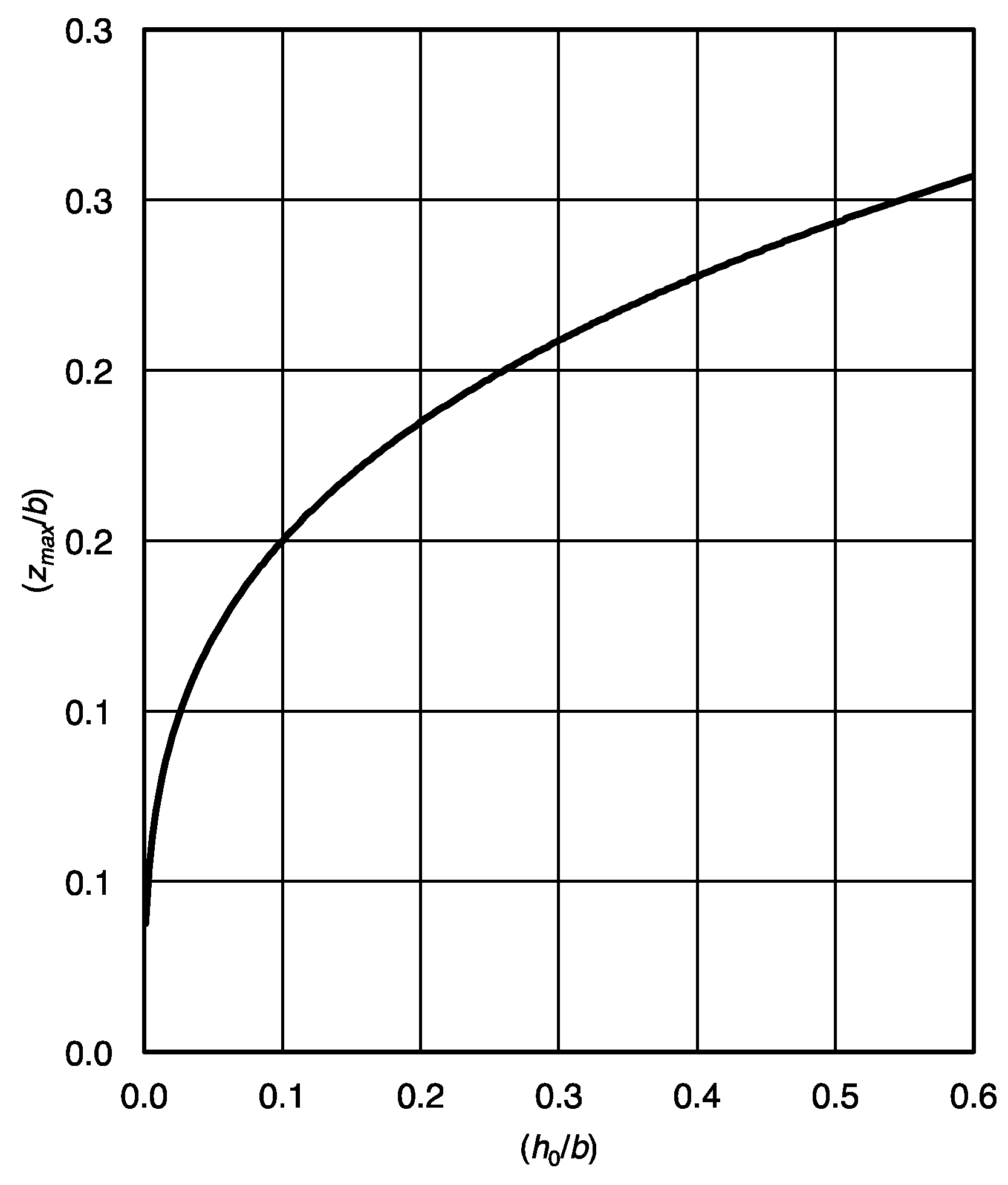
Basic design curve for depth of scour (rectangular piers at zero angle of attack) according to Lausen and Toch [12].
Figure 11.
Basic design curve for depth of scour (rectangular piers at zero angle of attack) according to Lausen and Toch [12].

Figure 12.
Distribution of the numerical value range of the function parameters in Monte Carlo sampling method: (a) Begam (1) formula (Dąbkowski et al. [5]), (b) Laursen & Toch (6) formula [12].

Figure 13.
Mean relative error δ for simulated th and k parameters using Begam formula (Equation (1)).
Figure 13.
Mean relative error δ for simulated th and k parameters using Begam formula (Equation (1)).

Figure 14.
Mean relative error δ for K0 parameter using formula included in Regulation (Journal of Laws 2000 No. 63, item 735) Equation (10).
Figure 14.
Mean relative error δ for K0 parameter using formula included in Regulation (Journal of Laws 2000 No. 63, item 735) Equation (10).

Figure 15.
Mean relative error δ for m and n parameters using Laursen & Toch formula (Equation (9)).
Figure 15.
Mean relative error δ for m and n parameters using Laursen & Toch formula (Equation (9)).

Figure 16.
Calculations results using Begam formula (Equations (1) and (11)), Regulation of the Polish Minister formula (Equations (8) and (12)), Laursen & Toch formula (Equations (9) and (13)).
Figure 16.
Calculations results using Begam formula (Equations (1) and (11)), Regulation of the Polish Minister formula (Equations (8) and (12)), Laursen & Toch formula (Equations (9) and (13)).


Table 1.
Main parameters of test series.
| Test Series | Qw | h0 | q | T | v | I0 | t |
|---|---|---|---|---|---|---|---|
| (m3 s−1) | (m) | (m3 s−1 m−1) | (h) | (m·s−1) | (‰) | (°C) | |
| 1 | 0.020 | 0.09 | 0.034 | 8.00 | 0.371 | 1.4 | 16.0 |
| 2 | 0.022 | 0.09 | 0.038 | 8.00 | 0.433 | 2.0 | 16.1 |
| 3 | 0.023 | 0.12 | 0.040 | 7.00 | 0.330 | 0.7 | 16.0 |
| 4 | 0.025 | 0.10 | 0.043 | 10.50 | 0.449 | 2.7 | 16.4 |
| 5 | 0.025 | 0.11 | 0.043 | 8.50 | 0.392 | 1.5 | 16.0 |
| 6 | 0.027 | 0.09 | 0.047 | 8.00 | 0.548 | 3.4 | 16.0 |
| 7 | 0.028 | 0.07 | 0.048 | 7.50 | 0.690 | 3.7 | 15.9 |
| 8 | 0.028 | 0.10 | 0.048 | 8.00 | 0.483 | 2.1 | 15.8 |
| 9 | 0.029 | 0.13 | 0.050 | 8.50 | 0.385 | 0.8 | 16.1 |
| 10 | 0.030 | 0.09 | 0.052 | 9.50 | 0.556 | 3.4 | 16.0 |
| 11 | 0.030 | 0.15 | 0.052 | 9.50 | 0.345 | 0.7 | 16.0 |
| 12 | 0.033 | 0.11 | 0.057 | 8.00 | 0.517 | 2.9 | 16.1 |
| 13 | 0.035 | 0.09 | 0.060 | 8.50 | 0.649 | 4.7 | 16.0 |
| 14 | 0.036 | 0.10 | 0.062 | 9.50 | 0.621 | 3.3 | 15.6 |
| 15 | 0.036 | 0.12 | 0.062 | 7.50 | 0.517 | 3.1 | 16.5 |
| 16 | 0.040 | 0.11 | 0.069 | 10.00 | 0.651 | 4.8 | 15.5 |
| 17 | 0.040 | 0.12 | 0.069 | 8.00 | 0.580 | 3.2 | 16.0 |
| 18 | 0.040 | 0.14 | 0.069 | 9.50 | 0.493 | 2.3 | 16.0 |
| 19 | 0.043 | 0.10 | 0.074 | 9.50 | 0.741 | 2.4 | 16.0 |
Qw—water discharge (m3 s−1); h0—water depth (m); q—unit discharge (m3 s−1 m−1); T—duration of experimental series (h); v—average water velocity (m·s−1); I0—initial water surface gradient (-); t—medium temperature of water (°C).
Table 2.
Computational parameters of the Equation (1) Begam’s formula after Dąbkowski et al. [5].
Table 2.
Computational parameters of the Equation (1) Begam’s formula after Dąbkowski et al. [5].
| Measurement Series Number | vn | w | K | ||
|---|---|---|---|---|---|
| (-) | (-) | (m s−1) | (m s−1) | (-) | |
| 1 | 0.538 | 0.105 | 0.345 | 0.098 | 1.00 |
| 2 | 0.538 | 0.105 | 0.345 | 0.098 | 1.00 |
| 3 | 0.568 | 0.110 | 0.341 | 0.098 | 1.00 |
| 4 | 0.420 | 0.085 | 0.367 | 0.098 | 1.00 |
| 5 | 0.472 | 0.094 | 0.357 | 0.098 | 1.00 |
| 6 | 0.521 | 0.102 | 0.348 | 0.098 | 1.00 |
| 7 | 0.538 | 0.105 | 0.345 | 0.098 | 1.00 |
| 8 | 0.455 | 0.091 | 0.360 | 0.098 | 1.00 |
| 9 | 0.714 | 0.134 | 0.322 | 0.098 | 1.00 |
| 10 | 0.417 | 0.084 | 0.368 | 0.098 | 1.00 |
| 11 | 0.455 | 0.091 | 0.360 | 0.098 | 1.00 |
| 12 | 0.500 | 0.099 | 0.352 | 0.098 | 1.00 |
| 13 | 0.500 | 0.099 | 0.352 | 0.098 | 1.00 |
| 14 | 0.417 | 0.084 | 0.368 | 0.098 | 1.00 |
| 15 | 0.333 | 0.069 | 0.389 | 0.098 | 1.00 |
| 16 | 0.385 | 0.079 | 0.375 | 0.098 | 1.00 |
| 17 | 0.357 | 0.074 | 0.382 | 0.098 | 1.00 |
| 18 | 0.588 | 0.114 | 0.338 | 0.098 | 1.00 |
| 19 | 0.500 | 0.099 | 0.352 | 0.098 | 1.00 |
b—width of pier (m); h0—water depth (m); —dimensionless coefficient calculated from the formula Equation (2) (-); vn—non-washable velocity, for non-cohesive soil calculated from Studenčníkov’s formula Equation (3) (m s−1); w—hydraulic feature of medium sized grains calculated from the formula Equation (4) (m s−1); K—coefficient calculated from the formula Equation (5) (-).
Table 3.
Chosen pier construction types and K1 parameter value (in accordance with Journal of Laws [11]).
Table 3.
Chosen pier construction types and K1 parameter value (in accordance with Journal of Laws [11]).
| Type | Pier Scheme | K1 | Type | Pier Scheme | K1 |
|---|---|---|---|---|---|
| A |  | 8.5 | C |  | 10.0 |
| B |  | 10.0 | D |  | 6.5 |
h0—water depth (m); zmax—maximal scour depth (m); v—average stream velocity (m s−1); —the angle of deviation of the axis of the support from the direction of water inflow (°); L—the length of a pillar or set of pillars (m); b—the width of the pier (m).
Table 4.
Permissible scour degree [11].
Table 4.
Permissible scour degree [11].
| No. | Type of Support Foundation | Shape within the Scour Boundary | |
|---|---|---|---|
| Non-Streamlined | Semi-Streamlined | ||
| 1 | Massive deep foundations, on large diameter piles and foundation directly on rocks | 1.3 | 1.4 |
| 2 | Foundations on piles in a sheet piling | 1.1 | 1.25 |
| 3 | Foundations on piles without a sheet piling | 1.0 | 1.1 |
| 4 | Foundation directly on the ground | 1.0 | 1.0 |
Table 5.
Computational parameters of the Equation (6) (in accordance with Journal of Laws of 2000 No. 63, item 735 [11]).
Table 5.
Computational parameters of the Equation (6) (in accordance with Journal of Laws of 2000 No. 63, item 735 [11]).
| Measurement Series Number: | (v2/gbz) | K2 | hr | (hr/bz) | K3 |
|---|---|---|---|---|---|
| (-) | (-) | (m) | (-) | (-) | |
| 1 | 0.280 | 0.66 | 0.093 | 1.9 | 0.337 |
| 2 | 0.382 | 0.62 | 0.088 | 1.8 | 0.366 |
| 3 | 0.223 | 0.69 | 0.120 | 2.4 | 0.218 |
| 4 | 0.411 | 0.61 | 0.096 | 1.9 | 0.321 |
| 5 | 0.313 | 0.64 | 0.110 | 2.2 | 0.256 |
| 6 | 0.611 | 0.57 | 0.085 | 1.7 | 0.384 |
| 7 | 0.970 | 0.52 | 0.070 | 1.4 | 0.488 |
| 8 | 0.475 | 0.60 | 0.100 | 2.0 | 0.301 |
| 9 | 0.302 | 0.64 | 0.130 | 2.6 | 0.185 |
| 10 | 0.631 | 0.57 | 0.093 | 1.9 | 0.337 |
| 11 | 0.242 | 0.67 | 0.150 | 3.0 | 0.132 |
| 12 | 0.545 | 0.59 | 0.110 | 2.2 | 0.256 |
| 13 | 0.858 | 0.54 | 0.093 | 1.9 | 0.337 |
| 14 | 0.785 | 0.55 | 0.100 | 2.0 | 0.301 |
| 15 | 0.545 | 0.59 | 0.120 | 2.4 | 0.218 |
| 16 | 0.863 | 0.54 | 0.106 | 2.1 | 0.273 |
| 17 | 0.685 | 0.56 | 0.119 | 2.4 | 0.221 |
| 18 | 0.495 | 0.60 | 0.140 | 2.8 | 0.157 |
| 19 | 1.121 | 0.51 | 0.100 | 2.0 | 0.301 |
v—average stream velocity (m s−1); g—gravity acceleration (m s−2); bz—substitutional pier width (m); K2—coefficient according to Figure 8 (-), hr—water depth over eroded bed (m); K3—coefficient according to Equation (7) (-).
Table 6.
Shape coefficients Ks for various nose pier form [12].
Table 6.
Shape coefficients Ks for various nose pier form [12].
| Nose Pier Form | Length-Width Ratio | Shape | Ks |
|---|---|---|---|
| Rectangular | - |  | 1.00 |
| Semicircular | - |  | 0.90 |
| Elliptic | 2:1 |  | 0.80 |
| Elliptic | 3:1 |  | 0.75 |
| Lenticular | 2:1 |  | 0.80 |
| Lenticular | 3:1 |  | 0.70 |
Table 7.
Monte Carlo sampling assumptions summary table.
| Formula Parameters Summary Set: | |||||
|---|---|---|---|---|---|
| Begam Equation (1) | Regulation of the Polish Minister Equation (6) | Laursen & Toch Equation (9) | |||
| th | k | K0 | m | n | |
| Parameter default value | 7.83 | 0.0177 | 1.00 | 1.50 | 0.30 |
| Range (%) | 7.83 ± 64% | (56%–2727%) | 1.00 ± 50% | 1.30 ± 33% | 0.30 ± 50% |
| Range (-) | 2.83–12.83 | 0.01–0.50 | 0.50–1.50 | 1.00–2.00 | 0.15–0.45 |
| No. of combinations | 10,000 | 101 | 10,000 | ||
Table 8.
Measured and calculated scour depth results.
| No. of Measurement Series | zmax Value | ||||||
|---|---|---|---|---|---|---|---|
| Begam Formula | Regulation of the Polish Minister Formula | Laursen & Toch Formula | |||||
| Laboratory Measurement | Equation (1) th = 7.83 k = 0.0177 | Equation (11) th = 7.75 k = 0.2326 | Equation (8) K0 = 1.00 | Equation (12) K0 = 0.93 | Equation (9) m = 1.50 n = 0.30 | Equation (13) m = 1.64 n = 0.15 | |
| (m) | (m) | (m) | (m) | ||||
| 1 | 0.0806 | 0.0673 | 0.0694 | 0.0456 | 0.0424 | 0.0813 | 0.0810 |
| 2 | 0.0767 | 0.0671 | 0.0765 | 0.0678 | 0.0630 | 0.0800 | 0.0803 |
| 3 | 0.0653 | 0.0705 | 0.0657 | 0.0265 | 0.0246 | 0.0878 | 0.0842 |
| 4 | 0.0776 | 0.0684 | 0.0788 | 0.0686 | 0.0638 | 0.0821 | 0.0814 |
| 5 | 0.0833 | 0.0698 | 0.0726 | 0.0449 | 0.0417 | 0.0855 | 0.0831 |
| 6 | 0.0903 | 0.0676 | 0.0899 | 0.1134 | 0.1054 | 0.0791 | 0.0799 |
| 7 | 0.0952 | 0.0662 | 0.1057 | 0.1957 | 0.1820 | 0.0747 | 0.0776 |
| 8 | 0.0729 | 0.0693 | 0.0830 | 0.0790 | 0.0735 | 0.0831 | 0.0819 |
| 9 | 0.0816 | 0.0721 | 0.0724 | 0.0368 | 0.0343 | 0.0899 | 0.0852 |
| 10 | 0.0905 | 0.0690 | 0.0913 | 0.1110 | 0.1032 | 0.0813 | 0.0810 |
| 11 | 0.0849 | 0.0737 | 0.0681 | 0.0238 | 0.0221 | 0.0939 | 0.0870 |
| 12 | 0.0840 | 0.0710 | 0.0874 | 0.0865 | 0.0804 | 0.0855 | 0.0831 |
| 13 | 0.1243 | 0.0698 | 0.1023 | 0.1500 | 0.1395 | 0.0813 | 0.0810 |
| 14 | 0.1268 | 0.0706 | 0.0993 | 0.1320 | 0.1227 | 0.0831 | 0.0819 |
| 15 | 0.0856 | 0.0722 | 0.0878 | 0.0815 | 0.0758 | 0.0878 | 0.0842 |
| 16 | 0.1211 | 0.0717 | 0.1031 | 0.1390 | 0.1293 | 0.0846 | 0.0826 |
| 17 | 0.0955 | 0.0727 | 0.0951 | 0.1022 | 0.0951 | 0.0876 | 0.0841 |
| 18 | 0.0797 | 0.0741 | 0.0854 | 0.0661 | 0.0614 | 0.0919 | 0.0861 |
| 19 | 0.1313 | 0.0717 | 0.1135 | 0.1823 | 0.1695 | 0.0831 | 0.0819 |
| Measurement uncertainty uc(y) | 4.63% | 4.63% | 14.5% | 14.5% | 0.54% | 0.54% | |
| Mean Squared Error MSE | 0.00081 | 0.00014 | 0.01609 | 0.01388 | 0.00037 | 0.00035 | |
| Average relative error δ | 21.6% | 8.8% | 30.1% | 28.5% | 15.3% | 13.8% | |
© 2020 by the authors. Licensee MDPI, Basel, Switzerland. This article is an open access article distributed under the terms and conditions of the Creative Commons Attribution (CC BY) license (http://creativecommons.org/licenses/by/4.0/).
Share and Cite
MDPI and ACS Style
Kiraga, M.; Urbański, J.; Bajkowski, S. Adaptation of Selected Formulas for Local Scour Maximum Depth at Bridge Piers Region in Laboratory Conditions. Water 2020, 12, 2663. https://doi.org/10.3390/w12102663
AMA Style
Kiraga M, Urbański J, Bajkowski S. Adaptation of Selected Formulas for Local Scour Maximum Depth at Bridge Piers Region in Laboratory Conditions. Water. 2020; 12(10):2663. https://doi.org/10.3390/w12102663
Chicago/Turabian StyleKiraga, Marta, Janusz Urbański, and Sławomir Bajkowski. 2020. "Adaptation of Selected Formulas for Local Scour Maximum Depth at Bridge Piers Region in Laboratory Conditions" Water 12, no. 10: 2663. https://doi.org/10.3390/w12102663
Note that from the first issue of 2016, this journal uses article numbers instead of page numbers. See further details here.