Global Cyclone and Anticyclone Detection Model Based on Remotely Sensed Wind Field and Deep Learning


Navigation College, Dalian Maritime University, Dalian 116026, China
*
Author to whom correspondence should be addressed.
Remote Sens. 2020, 12(19), 3111; https://doi.org/10.3390/rs12193111
Submission received: 8 September 2020
/
Revised: 21 September 2020
/
Accepted: 21 September 2020
/
Published: 23 September 2020
(This article belongs to the Special Issue Artificial Intelligence for Weather and Climate)
Abstract
:Cyclone detection is a classical topic and researchers have developed various methods of cyclone detection based on sea-level pressure, cloud image, wind field, etc. In this article, a deep-learning algorithm is incorporated with modern remote-sensing technology and forms a global-scale cyclone/anticyclone detection model. Instead of using optical images, wind field data obtained from Mean Wind Field-Advanced Scatterometer (MWF-ASCAT) is utilized as the dataset for model training and testing. The wind field vectors are reconstructed and fed to the deep-learning model, which is built based on a faster-region with convolutional neural network (faster-RCNN). The model consists of three modules: a series of convolutional and pooling layers as the feature extractor, a region proposal network that searches for the potential areas of cyclone/anticyclone within the dataset, and the classifier that classifies the proposed region as cyclone or anticyclone through a fully-connected neural network. Compared with existing methods of cyclone detection, the test results indicate that this model based on deep learning is able to reduce the number of false alarms, and at the same time, maintain high accuracy in cyclone detection. An application of this method is presented in the article. By processing temporally continuous data of wind field, the model is able to track the path of Hurricane Irma in September, 2017. The advantages and limitations of the model are also discussed in the article.
1. Introduction
Cyclone detection is a classical yet still actively developing topic, since it provides the theoretical foundation for the responses of extreme weather condition, as well as studies of the Earth’s climate system. As the development of modern (especially satellite-based) remote sensing, detecting cyclones in the larger temporal and spatial scale has become a trend of relevant studies [1]. Traditional cyclone detection methods focus on the characteristics of a pressure gradient, and detect the cyclones by locating the low-pressure centers [2,3,4]. Rudeva and Gulev analyzed sea-level pressure (SLP) data over the northern hemisphere, based on which they detected cyclones by locating the minimum points of SLP [5]. Based on this method, Simmonds et al. proposed an automatic cyclone detection algorithm by comparing the Laplacian operator of SLP at each grid point to those at neighboring grid points [6]. Hanley and Caballero also developed an identification and tracking method that specifically recognized multicenter cyclones by examining the gradient of SLP and finding minimum points [7]. Although the minimum SLP method can effectively detect an ideal cyclone, the accuracy of the detection result is limited due to the lack of in situ data and ambiguities in satellite presentation.
Because the wind field of a cyclone has strong characteristics in geometric symmetry, the vector field formed by the wind speed certainly has the potential for detecting cyclones. Fluid dynamicists developed various methods of identifying a vortex core in the fluid field [8,9]. The Okubo–Weiss (OW) approach is one of the most well-known methods of distinguishing high vorticity zone within the flow field by calculating OW parameter using strain and vorticity of the velocity field as follows [10,11]:
where Ss and Sn are the shear and normal components of strain, and ω is the relative vorticity. They can be calculated using the following equations:
where U’ and V’ are the zonal and meridional components of the flow velocity; x and y represent the coordinates.
The OW parameter quantitatively describes the significance of rotation compared with deformation in the flow field. Generally, the vortex core is characterized as strong rotation, and has an OW parameter of negative value; while vortex ring is characterized as strong deformation, and has an OW parameter of positive value. The OW parameter that is close to 0 indicates the background with no vortex-shape events. By defining a threshold value W0, vortex core can be identified by searching for the areas with OW parameter that is smaller than the predefined threshold. This method has been widely used in oceanography and meteorology. For example, numerous studies have applied the OW approach on sea-level anomaly (SLA) data and developed identification models for oceanic eddies [12,13,14,15,16,17,18]. Similarly, a cyclone could be detected by examining the vorticity of the wind field, since the cyclone eyes usually have high vorticity [19]. Wong et al. studied the patterns of a spiraling vector field and developed a method of identifying a circulating center. They suggested that this method could potentially be applied to detect cyclone eyes [20]. Following this method, Inatsu proposed a cyclone identification method by comparing the vorticity field of the cyclone eyes with that of the neighborhoods [21]. With the data collected by modern remote-sensing techniques, researchers are able to identify cyclones in larger spatial scale. Zou et al. proposed an automatic cyclone detection algorithm using the wind vector obtained from the Quick Scatterometter (QuikSCAT) satellite [22]. Warunsin and Chitsobhuk further combined the wind data with cloud shape and developed a fuzzy inference system for cyclone detection [23]. However, such studies usually focus on a regional area, even with the data obtained at global scale [14,15,16,17]. This is partly because of the difficulties in determining the appropriate threshold W0 for the OW parameter at the global scale. In practice, the threshold W0 needs to be adjusted for different location and time when identifying vortex cores in large-scale [24] or time series [25] data. Other approaches are proposed by researchers in order to avoid using the regional threshold and overcome this limitation. For examples, Williams et al. simulated the physics and geometry of idealized vortex, and presented the R2 method, which determines how well an eddy confirms to the characteristics of an ideal Gaussian vortex through linear regression [26]. Peterson et al. conducted a large-scale simulation on oceanic eddies, and identified the simulated eddies using the R2 method [27]. Li et al. proposed an iterative algorithm for eddy detection, in which the eddy regions are separated from non-eddy regions through data segmentation, and then recognized using a density clustering method [28].
As in the development of artificial intelligence (AI) technology in the last decade, machine learning algorithm has been successfully applied in the subjects of object detection and pattern recognition owing to its ability to efficiently extract imagery information. In the subjects of oceanography and meteorology, state-of-the-art machine-learning algorithms have been applied to recognize the circulating pattern in a spiraling fluid field [29]. Moreover, deep convolutional neural network (DCNN) has been utilized to detect and classify objects in remote-sensing images [30,31]. Based on DCNN, researchers have successfully developed object detection models for land-use and land-cover [32,33], vegetation [34,35], urban commerce [36,37], transportation vehicles [38,39], etc. Similarly, attempts are made to detect cyclones based on cloud images. Lee and Liu classified the appearance of tropical cyclones in remote-sensing images into eight possible categories, and then trained the neural network based on this classification [40]. The drawback of using remote-sensing images as the training dataset of cyclone detection is that the appearance of some non-cyclone clouds is similar to those of cyclones. That fact negatively affects the accuracy of the identification model [41,42]. Bai et al., constructed and trained a deep-learning model for oceanic eddy detection using enhanced maps of a streampath, which are produced using ocean velocity field data [43]. Ho and Talukder conducted a series of studies and proposed automatic cyclone identification methods based on a support vector machine (SVM) and dominant wind direction (DOWD) classifier using the wind data from the QuikSCAT satellite [1,44,45]. They further combined the wind data from QuikSCAT and precipitation data from the Tropical Rainfall Measurement Mission (TRMM), and built a Cyclone Discovery Module (CDM) that was able to achieve accurate detection results [1,45]. These successful applications of machine learning illustrate its ability of analyzing complex systems that are not well understood, but with plenty of observations. With the extensive data collected by modern remote-sensing technology, obviously, the machine-learning method could be potentially applied to study the complex climate system, including cyclone and anticyclone.
In this study, a cross-boundary research is achieved by applying a state-of-the-art deep learning model into a classical research field. The wind field vector in the global scale is reconstructed to form the training and testing dataset for the deep-learning model, and the model is modified in order to work with wind field data. The deep-learning technology is expected to accomplish a large-scale cyclone/anticyclone detection that is difficult to achieve with traditional methods.
2. Methodology
2.1. Dataset Acquisition and Reconstruction
Instead of using optical remote-sensing images, wind speed data is utilized to construct the dataset. Specifically, mean wind fields (MWF) data obtained by the Advanced Scatterometer (ASCAT) is applied in this study. MWF-ASCAT wind field data cover the Earth’s surface between 80°N~80°S and 180°W~0°~180°E, with the spatial resolution of 0.25° × 0.25°. Their temporal coverage starts from March 2007. The daily average series data are used in this study. The MWF-ASCAT dataset contains 15 variables including: longitude, latitude, surface wind speed (m/s), eastward wind (m/s), northward wind (m/s), surface wind stress (Pa), horizontal surface wind divergence (1/s), horizontal wind stress curl (Pa/m), etc. Four of these variables are used in the study: northward wind and eastward wind are used to form the 2-layer dataset; latitude and longitude are used to locate the cyclone/anticyclone in the dataset.
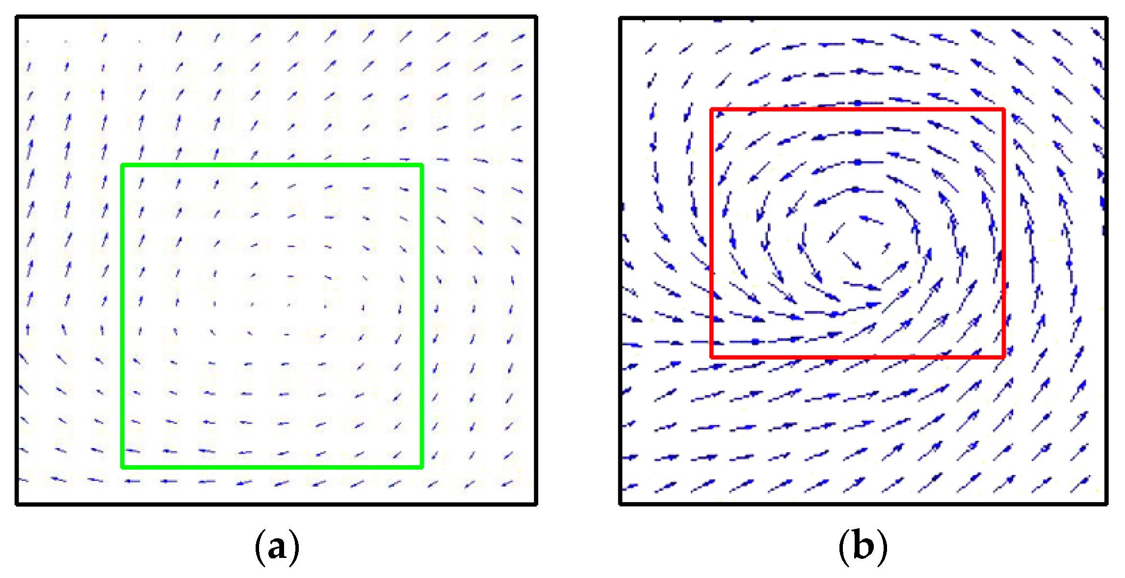
The training dataset is constructed by manually labelling the clockwise and anticlockwise cyclone within the dataset. Because the wind fields of cyclone and anticyclone rotate in the opposite directions in the northern and southern hemisphere, it is easier for the model to classify the wind fields as a clockwise or anticlockwise cyclone, and then determine whether they are cyclone or anticyclone based on their locations (clockwise cyclones in the southern hemisphere and anticlockwise cyclones in the northern hemisphere are classified as cyclones, and vice versa). Thus, the training dataset are classified into two categories: (1) Class 1: wind field of clockwise rotation; (2) Class 2: wind field of anticlockwise rotation. The examples of the wind fields that belong to the two categories are shown in Figure 1.
The cyclones and anticyclones in the dataset are selected from March 2007 to December 2014. The reconstructed dataset includes 700 examples from Class 1, and 800 examples from Class 2. We tried to avoid including the same cyclone that appeared in two consecutive days in the dataset. Moreover, we tried to balance the number of cyclones and anticyclones (828 cyclones and 672 anticyclones), as well as their locations (766 from the northern hemisphere and 734 from the southern hemisphere). The Visual Object Tagging Tool (VoTT) is used to label cyclones in the dataset (the code can be accessed from: https://github.com/microsoft/VoTT). Because it is much easier for human eyes to find rotational flow field on the figures of vector field rather than the 2-layer dataset of northward and eastward wind speed, the clockwise and anticlockwise cyclones are labelled on the image of the vector field (Figure 1) first. Then the labelling boxes are mapped onto the 2-layer dataset of the same dimension based on latitude and longitude information. The time and location of cyclones in the dataset are confirmed with the hurricane data from Unisys Weather.
2.2. Model Structures
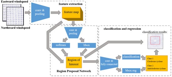
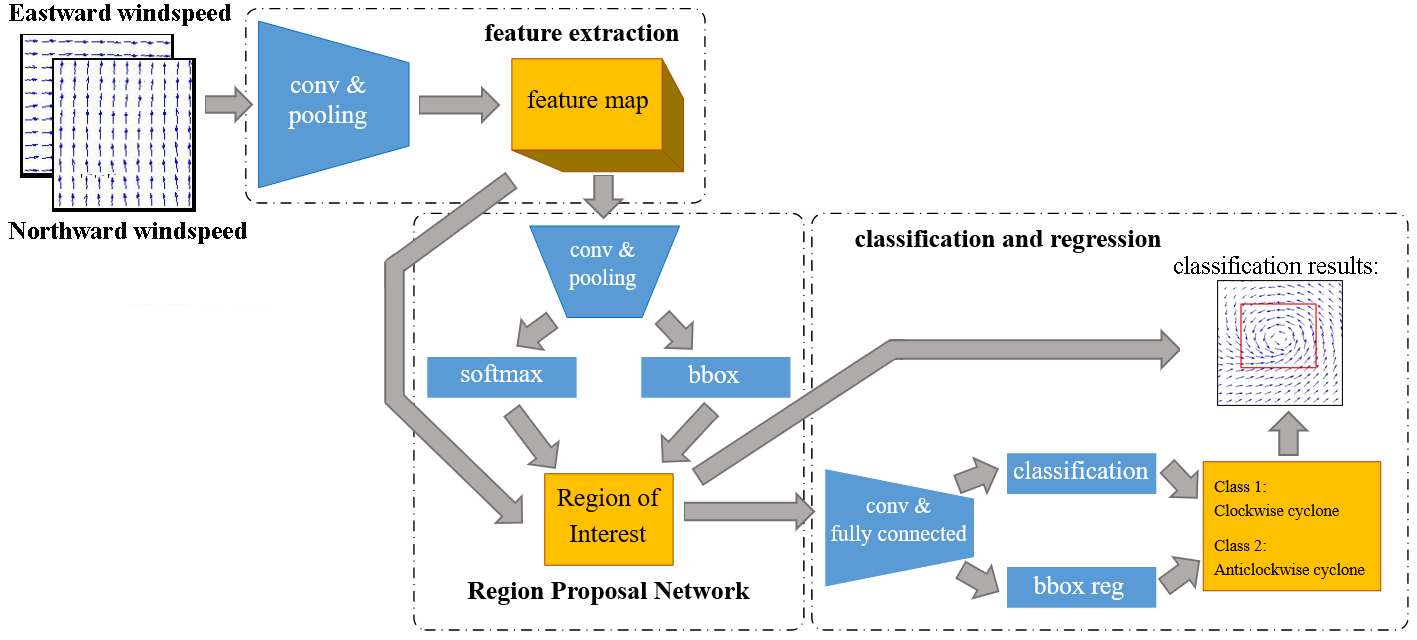
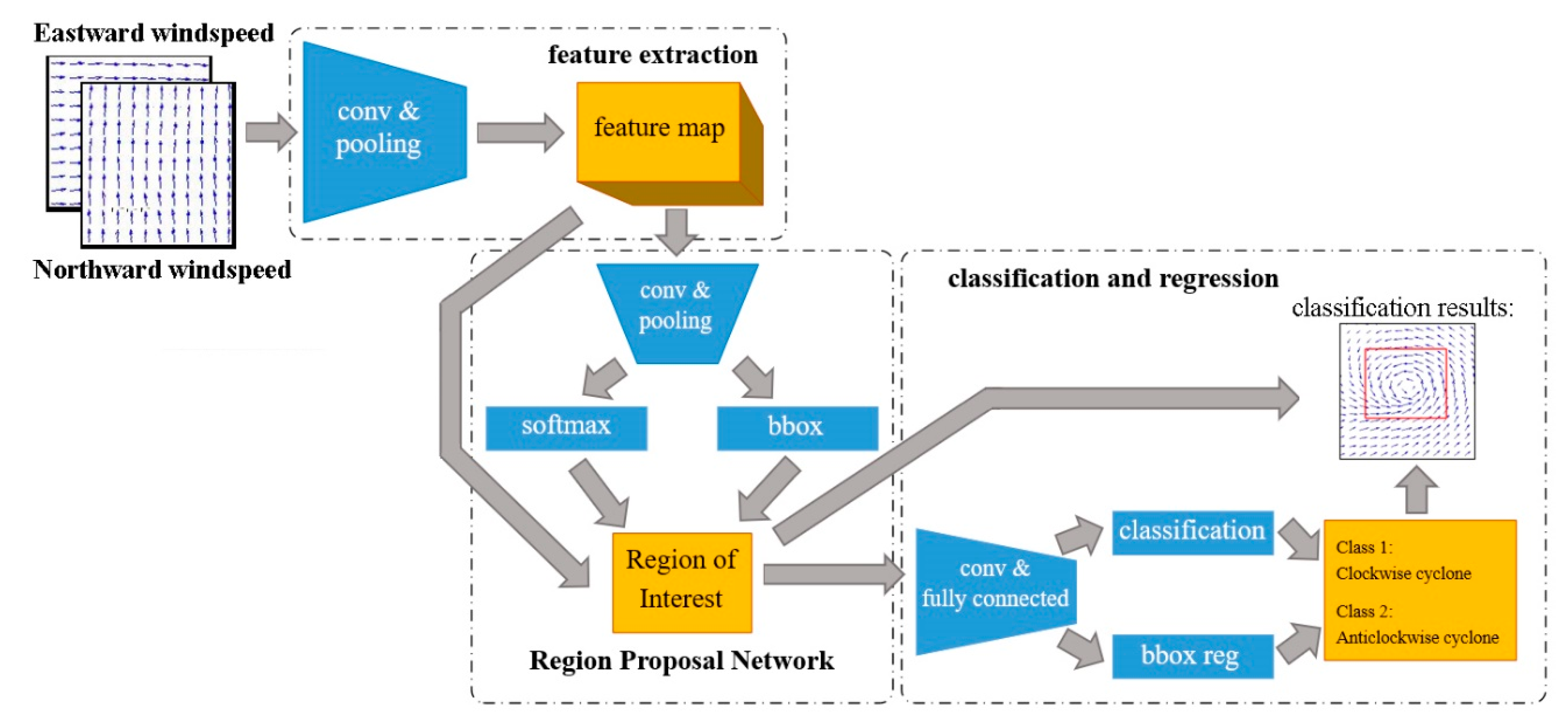
Various deep-learning models have been developed for object detection, including YOLO (you only look once) [46], SSD (single shot multibox detector) [47], and faster-RCNN (faster-region with convolutional neural network) [48]. In this study, we adopted the faster-RCNN algorithm to construct the model. As shown in Figure 2, the algorithm includes three parts: (1) the first part is a feature extractor, which is similar to the VGG-16 model [49] and consists of 5 convolutional layers and 5 pooling layers; (2) the second part is a region proposal network (RPN) that seeks for potential areas with cyclone and anticyclone in the wind field; (3) the third part is a classifier that classifies the proposed region into two categories (cyclone and anticyclone).
Because the faster-RCNN model is intended to detect objects in a red, green and blue (RGB) image, while the wind field dataset constructed in this study has a different structure from a RGB image, the feature extraction part needs to be modified in order to work with the wind field dataset. Unlike an RGB image that has the depth of three (representing the value of red, green, and blue, respectively), the wind field dataset has the depth of two, which represents northward wind and eastward wind respectively. Therefore, the input dimension of the convolutional layers in the feature extractor is adjusted in order to process the wind field data.
As shown in Figure 2, five convolution layers and pooling layers are applied on the reconstructed dataset and produce the feature maps. Rectified linear unit (ReLU) [50] is applied as the activation function between the convolutional and pooling layers. Based on these feature maps, RPN proposes candidate cyclone/anticyclone regions, of which the probability is estimated on a fixed set of anchors on different positions of the feature maps. According to the size of the cyclone/anticyclone, three types of anchor size are applied in the model: 4, 8, and 16, which represent 1°, 2°, and 4° on the Earth’s surface. For the anchor ratio, only 1:1 square is applied in the model because the shapes of cyclone/anticyclone are mostly close to a circle, and can be enclosed in a square region.
Softmax function is used to determine whether the region is positive or negative, and bounding box regression function is used to calibrate the location of the anchor. The calibrated positive regions of different sizes are then processed through another pooling layer and normalized as 5 × 5 feature maps. The feature maps are further processed through 2 convolutional layers and turned into vectors with a dimension of 1024 × 1 × 1. These vectors, together with the locations of the candidate regions, are fed to the classifier for cyclone/anticyclone classification.
In the classifier, the feature vectors (1024D) are sent to the fully-connected (FC) layers to make the prediction for each proposed region. The FC layers consist of an input layer, two hidden layers (each of which consists of 256 units), and an output layer. The activation function of hidden layers is also ReLU, while that of output layers is a sigmoid function.
2.3. Implementation Details
The model in this study is constructed and trained with Keras in the Tensorflow backend [51] and Python 3.6 environment. In terms of hyperparameter settings, the initial learning rate is set at 0.0001, and reduces at a factor of 10 after 10,000 iterations. The maximum number of iterations is set at 20,000. Non-maximum suppression (NMS) [48] is applied in the classifier to decide the prediction, and the intersection-over-union (IoU) thresholds of NMS are 0.75 and 0.25 for training and testing, respectively. The model is trained using the dataset built in the previous section. 70% of the wind field data are used for training, 10% of the data are used for validation, and 20% of the data are used for testing.
3. Results
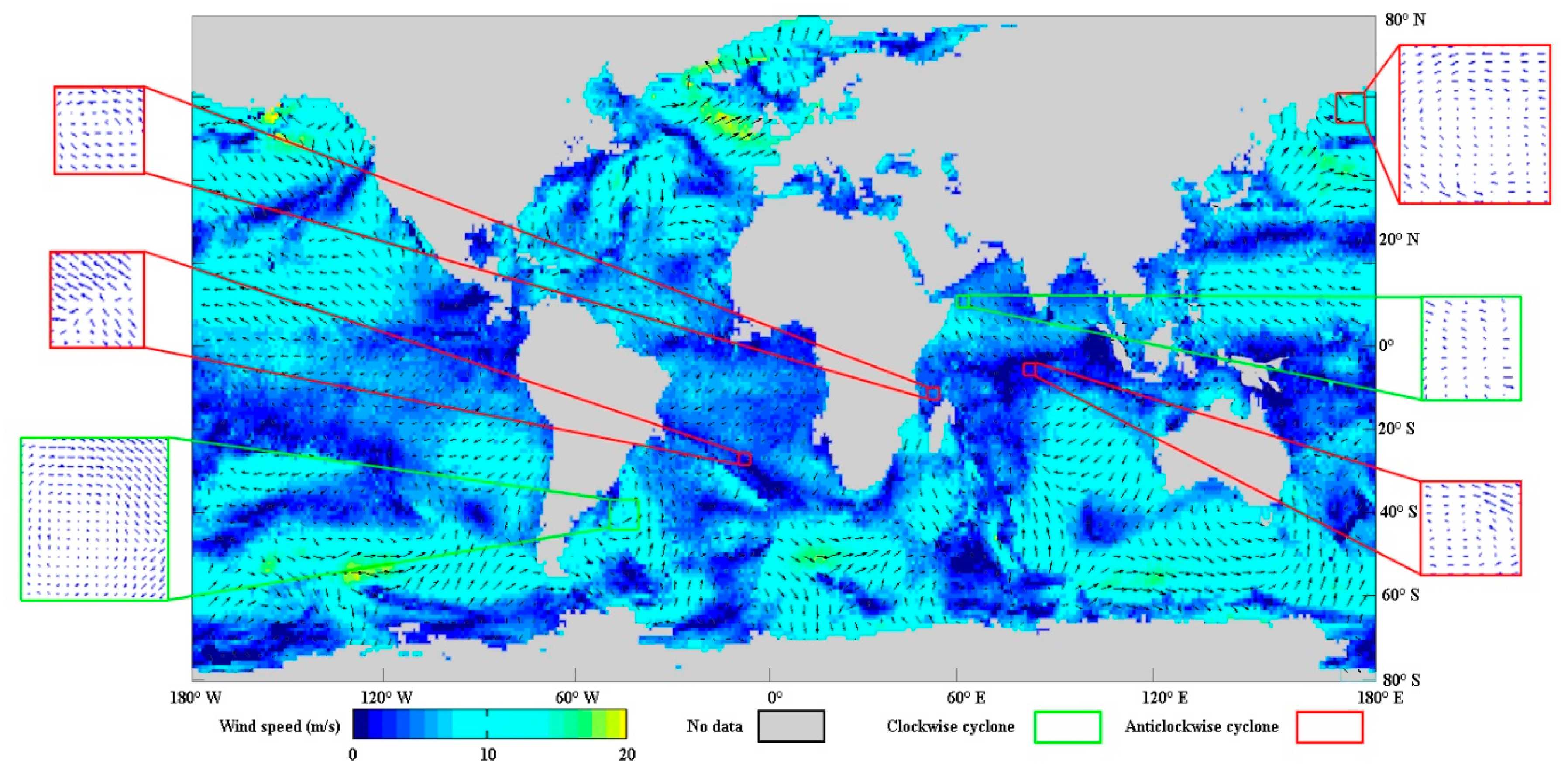
A performance experiment is conducted based on the global MWF-ASCAT data collected from 25 February 2020 to 5 March 2020 (these data are not included in the training or testing dataset). Figure 3 shows the clockwise and anticlockwise cyclones detected at a global scale on 25 February 2020. The results show the model is able to detect cyclones and anticyclones at different latitude.
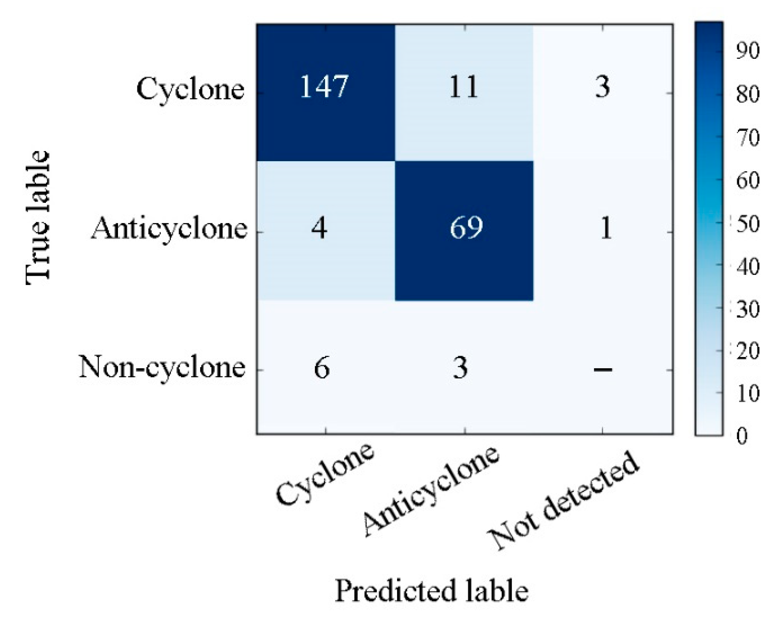
In order to verify the accuracy of the model, the results are evaluated by the standard performance measurements: true positive rate (TPR), true negative rate (TNR), false positive rate (FPR), and false negative rate (FNR). According to the wind field data of these 10 days, there are totally 161 cyclones and 74 anticyclones. The confusion matrix of the detection result is shown in Figure 4. Based on the confusion matrix, the corresponding performance measurements for cyclones and anticyclones are calculated in Table 1.
Typical examples of missing reports and false alarms are found and analyzed. Because MWF-ASCAT only provides wind field over the ocean surface, when the cyclone landed (Figure 5a), its wind field is not completely recorded in the dataset. As a result, the model fails to detect the cyclone. For the same reason, it can be inferred that when the cyclone or anticyclone locates at the boundary of the dataset (part of the wind field is cut off), it may not be detected by the model. This problem may be overcome by some data preprocessing techniques. For example, the missing wind field in the areas of small island may be filled with objectively-mapped wind vectors, or spatial interpolation of neighboring wind field; and the wind field that is cut off by the 180° meridian may be supplied by duplicating part of the wind field (e.g., 2° to 4° in longitude) on the boundary of the other side of the dataset. However, the cyclones and anticyclones within the duplicated zone are likely to be detected twice.
According to the false alarm shown in Figure 5b, some cyclone-like turbulences are recognized as cyclones. Such turbulences are likely to be caused by a tropical depression that is not strong enough to develop (or downgrades from) a cyclone, or a monsoon gyre at a specific time and location. These examples of missing reports indicated that the model may not be able to distinguish the wind rotation with high vorticity causing by non-cyclone event from actual cyclone.
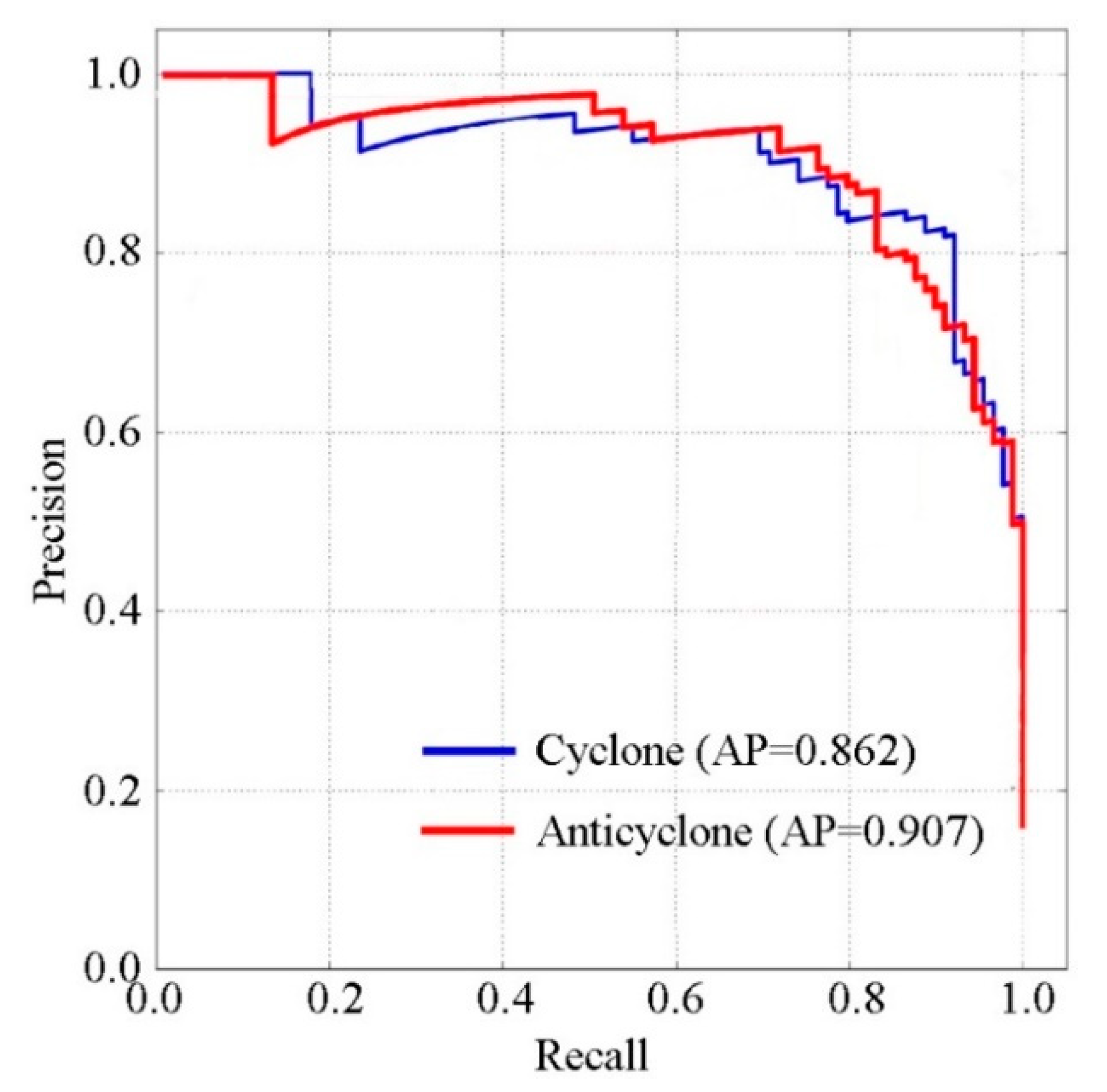
The accuracy of the detection results can also be evaluated through a precision-recall (PR) curve. According to the PR curve shown in Figure 6, it is found that the classification model is able to achieve accurate results on both cyclone and anticyclone—their average precision (AP) values are more than 0.85. It is also found that the high precision and recall values are achieved for both cyclone and anticyclone with the confidence over 0.9. Therefore, the proposed region with a confidence over 0.9 is preserved for the model training.
4. Discussion
4.1. Accuracy Analysis and Comparison
As shown in the PR curve (Figure 6), both cyclones and anticyclones can be effectively distinguished through the deep-learning model. The differences between the AP values of cyclone and anticyclone detection results are not significant, which means the model does not have bias on the detection of either type of cyclone.
The algorithm proposed in this article is compared with the SVM model proposed by Ho and Talukder [44]. As indicated in Table 2, both of these two methods are able to achieve good results in cyclone detection. It should be noted that our method achieves a significantly better performance on TNR compared with that based on the SVM method. This is possibly because the region of interest (ROI) for a potential cyclone is formed by a wind speed threshold in the SVM method, which means that non-cyclone areas with strong wind (these areas are commonly seen in the data) will be picked as a potential cyclone region for the classifier. In our method, the potential cyclone regions are formed from the positive anchors proposed by RPN (see Section 2.2 for details). As a result, less ROI is likely to be formed and tested for the classifier. In that vein, it is expected that the model would be more efficient, and less non-cyclone events would be identified from the dataset. Therefore, compared with the existing cyclone detection model based on machine learning, this method based on deep learning is able to produce fewer false alarms, and at the same time, maintain high sensitivity and accuracy.
4.2. Potential Application of the Model
As a global-scale, programmable tool with high efficiency and accuracy, the cyclone/anticyclone detection model based on deep learning proposed in this article is expected to be applied in large-scale studies on cyclones and climate patterns. For example, by detecting cyclones in the global range with high accuracy and efficiency, it is possible to construct a comprehensive dataset of cyclone occurrences in a large temporal and spatial scale. By statistically analyzing this dataset, further studies on the patterns of cyclone occurrences could be realized.
Another application of this model would be tracking the cyclone path. By processing the temporally continuous data using the cyclone detection model, the locational information of the cyclone can be obtained through the proposed regions and the movement of a cyclone can be captured by the model.
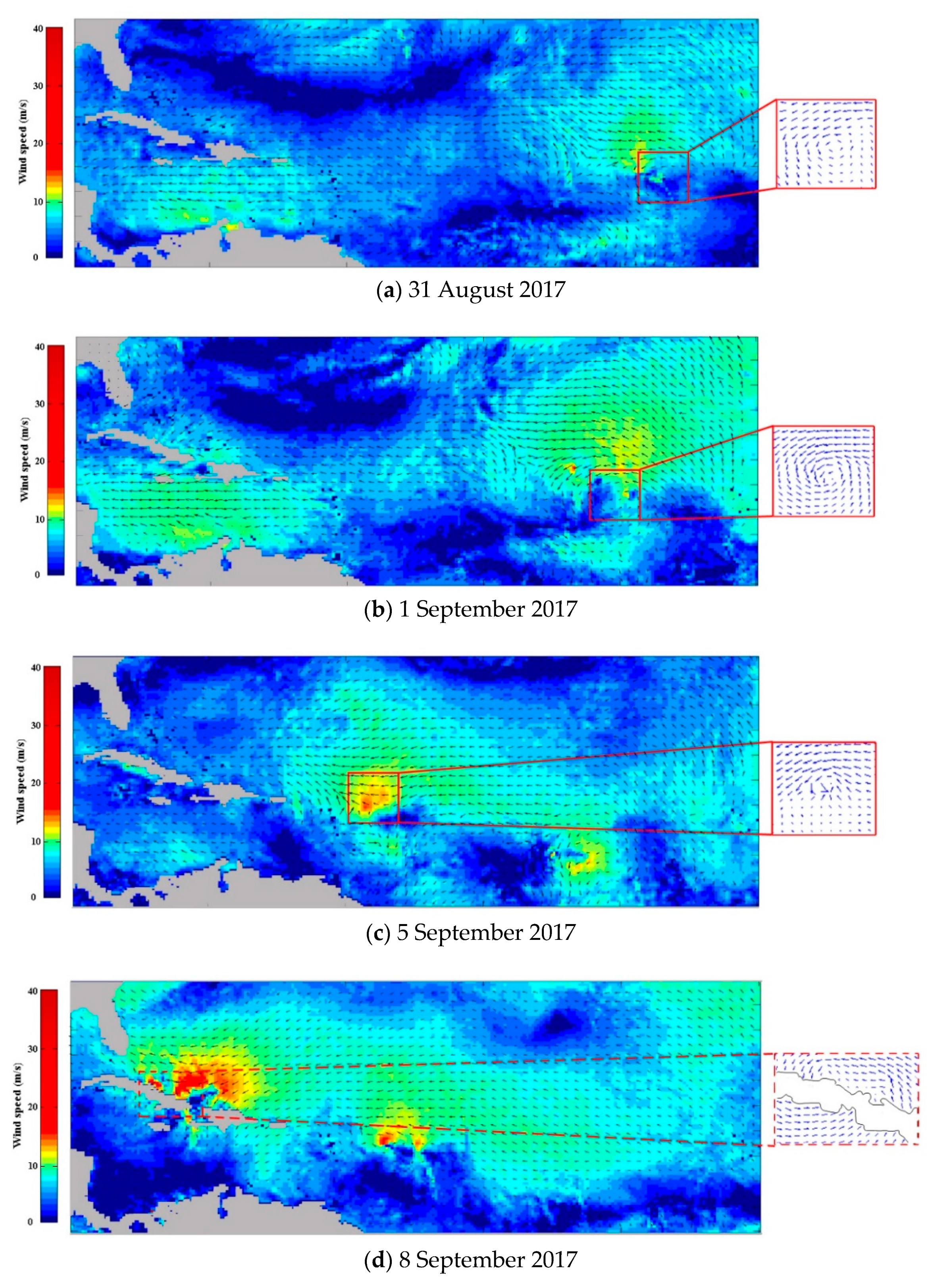
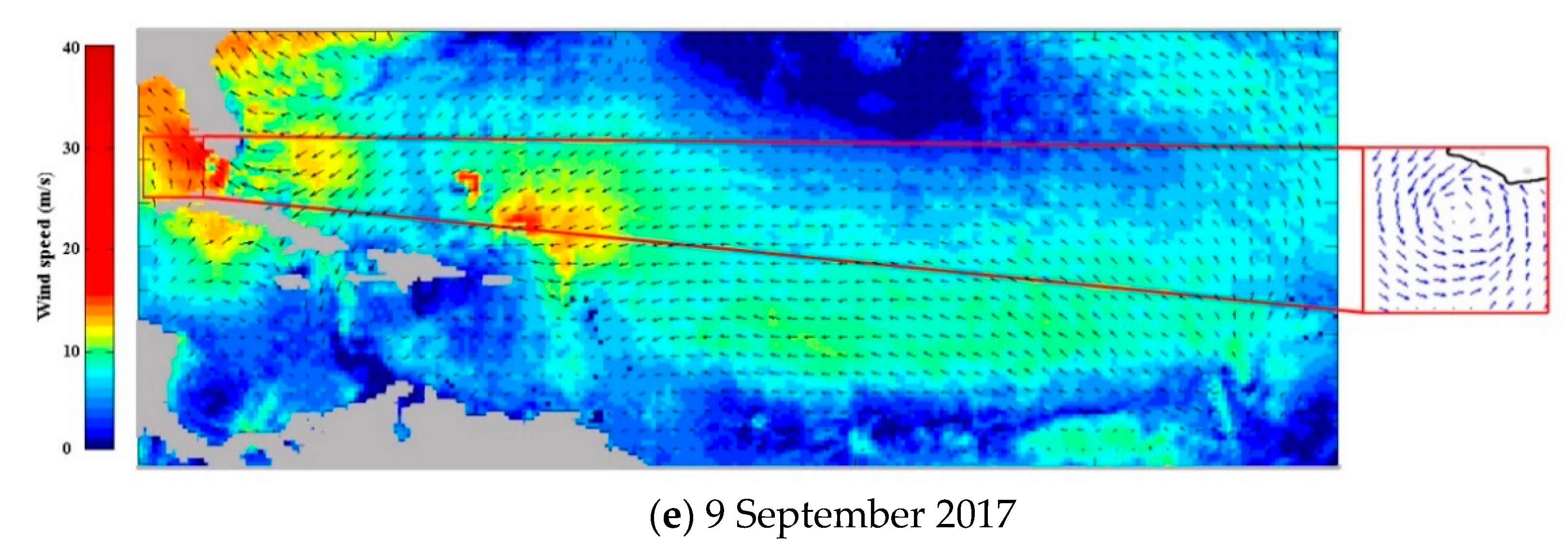
As an example, the path of Hurricane Irma that occurred in September 2017 was tracked with this model. As the results show in Figure 7a, hurricane Irma was detected when it was only a tropical storm. Moreover, its moving path was also tracked: it moved westward from the west Atlantic Ocean, flew over Cuba, turned northward and finally landed on Florida, United States. The cyclone was not detected by the model in Figure 7d, because the hurricane landed on Cuba and the MWF-ASCAT does not include wind field data on land. Therefore, ideally, the wind field dataset that covers both land and ocean area is preferable for accurate cyclone tracking.
It should be noted that although this model is able to detect cyclone regions, it cannot accurately determine cyclone eyes. However, it is more important to identify the location of a cyclone eye for cyclone tracking. Thus, in order to develop a completed cyclone tracking model, an additional algorithm for locating a cyclone eye needs to be integrated in the deep-learning model. Considering the symmetric geometry of the cyclone, one of the easiest algorithms is probably making the center of the proposed region as the location of the cyclone eye. However, this is not tested and may not be very accurate, since the shape of the cyclone could still be irregular. Combining the deep-learning model with an appropriate algorithm for locating cyclone eyes and developing a global cyclone tracking model would be the topic of our near future study.
Moreover, for the purpose of cyclone analysis, the resolution of the satellite data (0.25° × 0.25° in this study) is sometimes too coarse to determine the exact location of the cyclone eyes. Therefore, the model developed in this study is more suitable and effective for the application of cyclone detection in a large spatial and temporal scale without strict requirements on the spatial resolution of the detection result, or some census-type of studies over a large area or long period. This problem is also expected to be solved by providing high-resolution wind field data, which could potentially be achieved through the development of modern remote-sensing technology.
5. Conclusions
A novel approach for cyclone and anticyclone detection based on wind-field data and deep learning is presented in this study. This model learns to search for potential areas of cyclone and anticyclone events through RPN, and then perform the classification based on DCNN. The feature of the wind vector field is extracted by convolutional layers, and the spiral pattern of a cyclone is recognized and captured as proposed regions, which are further classified through FC neural networks.
The model proposed in this study is compared with existing methods of cyclone detection based on machine learning. Unlike the existing methods that generate ROI based on the wind speed threshold, our algorithm adopts faster-RCNN, which proposes ROI using RPN. Because the potential areas of cyclone events are more accurately captured, the efficiency of the model is improved and the number of false alarms is reduced.
In that vein, it is expected that this model is a promising tool for the pattern analysis of cyclone occurrences in a larger temporal and spatial scale. Utilizing the computational power of a state-of-the-art machine-learning algorithm, we hope this cyclone detection model can help propel large-scale studies on cyclone occurrences and climate patterns.
Author Contributions
Conceptualization, Y.L. and M.X.; methodology, M.X.; software, M.X. and K.C.; validation, M.X. and K.C.; formal analysis, M.X.; writing—original draft preparation, M.X.; writing—review and editing, M.X., Y.L., K.C.; supervision, Y.L. All authors have read and agreed to the published version of the manuscript.
Funding
This research was funded in part by China National Key R&D Program grant number 2018YFB1600400 and 2020YFE0201500, and in part by China Postdoctoral Science Foundation, grant number 2020M670730.
Acknowledgments
The authors would like to thank the European Remote Sensing (ERS) program of the European Space Agency for providing free satellite data, and the National Centers for Environmental Prediction (NCEP) for providing free hurricane and storm data. The authors would also like to thank Qinglai Yu, Zhanjun Ma, Wenbo Zheng from Dalian Maritime University for their help in preparing the training dataset. The authors are grateful to the three anonymous reviewers for their constructive comments on this work.
Conflicts of Interest
The authors declare no conflict of interest.
References
- Ho, S.-S.; Talukder, A. Automated cyclone discovery and tracking using multiple knowledge sharing in multiple heterogeneous satellite data. In Proceedings of the 14th ACM SIGKDD International Conference on Knowledge Discovery and Data Mining, Las Vegas, MV, USA, 24–27 August 2009; pp. 928–936. [Google Scholar]
- Barnett, T.P. Variations in near global sea level pressure. J. Atmos. Sci. 1985, 42, 478–501. [Google Scholar] [CrossRef] [Green Version]
- Sinclair, M.R. Objective identification of cyclones and their circulation intensity and climatology. Wea Forecast. 1997, 12, 595–612. [Google Scholar] [CrossRef]
- Pinto, J.G.; Spangehl, T.; Ulbrich, U.; Speth, P. Sensitivities of a cyclone detection and tracking algorithm: Individual tracks and climatology. Meteorol. Z. 2005, 14, 823–838. [Google Scholar] [CrossRef]
- Rudeva, I.; Gulev, S.K. Climatology of cyclone size characteristics and their changes during the cyclone life cycle. Mon. Wea. Rew. 2007, 135, 2568–2587. [Google Scholar] [CrossRef]
- Simmonds, I.; Burke, C.; Keay, K. Arctic climate change as manifest in cyclone behavior. J. Climate 2008, 21, 5777–5796. [Google Scholar] [CrossRef]
- Hanley, J.; Caballero, R. Objective identification and tracking of multicentre cyclones in the ERA-Interim reanalysis dataset. Q. J. R. Meteorol. Soc. 2012, 138, 612–625. [Google Scholar] [CrossRef]
- Theisel, H.; Sahner, J.; Weinkauf, T.; Hega, H.-C.; Seidel, H.-P. Extraction of parallel vector surfaces in 3D time-dependent fields and application to vortex core line tracking. In Proceedings of the IEEE Visualization Conference, Minneapolis, MN, USA, 23–28 October 2005; pp. 631–638. [Google Scholar]
- Liu, S.-D.; Shi, S.-Y.; Liu, S.-K.; Fu, Z.-T.; Liang, F.-M.; Xin, G.-J. Vortex of fluid field as viewed from curvature. Commun. Theor. Phys. 2005, 43, 604–606. [Google Scholar]
- Okubo, A. Horizontal dispersion of floatable particles in the vicinity of velocity singularities such as convergences. Deep Sea Res. Oceanogr. Abs. 1970, 17, 445–454. [Google Scholar] [CrossRef]
- Weiss, J. The dynamics of enstrophy transfer in two-dimensional hydrodynamics. Physica D 1991, 48, 273–294. [Google Scholar] [CrossRef]
- Isern-Fontanet, J.; Garcia-Ladona, E.; Font, J. Identification of marine eddies from altimetric maps. J. Atoms. Ocean. Technol. 2003, 20, 772–778. [Google Scholar] [CrossRef]
- Morrow, R.; Birol, F.; Griffin, D.; Sudre, J. Divergent pathways of cyclonic and anti-cyclonic ocean eddies. Geophys. Res. Lett. 2004, 31, L24311. [Google Scholar] [CrossRef]
- Isern-Fontanet, J.; Garcia-Ladona, E.; Font, J. Vortices of Mediterranean Sea: An altimetric Prospective. J. Phys. Oceanogr. 2006, 36, 87–103. [Google Scholar] [CrossRef] [Green Version]
- Henson, S.A.; Thomas, A.C. A census of oceanic anticyclonic eddies in the Gulf of Alaska. Deep Sea Res. Pt. I 2008, 55, 163–176. [Google Scholar] [CrossRef]
- Xiu, P.; Chai, F.; Shi, L.; Xue, H.; Chao, Y. A census of eddy activities in the South China Sea during 1993–2007. J. Geophys. Res. 2010, 115, C03012. [Google Scholar] [CrossRef] [Green Version]
- Nan, F.; He, Z.; Zhou, H.; Wang, D. Three long-lived anticyclonic eddies in the northern South China Sea. J. Geophys. Res. 2011, 116, C05002. [Google Scholar] [CrossRef]
- Yi, J.; Du, Y.; He, Z.; Zhou, C. Enhancing the accuracy of automatic eddy detection and the capability of recognizing the multi-core structures from maps of sea level anomaly. Ocean. Sci. 2014, 10, 39–48. [Google Scholar] [CrossRef] [Green Version]
- Post, F.H.; Vrolijk, B.; Hauser, H.; Laramee, R.S.; Doleisch, H. The state of the art in flow visualization: Feature extraction and tracking. Comput. Graph. Forum 2003, 22, 1–17. [Google Scholar] [CrossRef] [Green Version]
- Wong, K.-Y.; Yip, C.-L. Identifying centers of circulating and spiraling vector field patterns and its applications. Pattern Recogn. 2009, 42, 1371–1387. [Google Scholar] [CrossRef]
- Inatsu, M. The neighbor enclosed area tracking algorithm for extratropical wintertime cyclones. Atmos. Sci. Lett. 2009, 10, 267–272. [Google Scholar] [CrossRef]
- Zou, J.; Lin, M.; Xie, X.; Lang, S.; Cui, S. Automated typhoon identification from QuikSCAT wind data. In Proceedings of the IEEE International Geoscience and Remote Sensing Symposium, Honolulu, HI, USA, 25–30 July 2010; pp. 4158–4161. [Google Scholar]
- Warunsin, K.; Chitsobhuk, O. Storm eye identification using fuzzy inference system. Int. J. Innov. Comput. Info. Control. 2016, 12, 1333–1349. [Google Scholar]
- Chelton, D.; Schlax, M.; Samelson, R.; de Szoeke, R. Global observations of large oceanic eddies. Geophys. Res. Lett. 2007, 34, L15606. [Google Scholar] [CrossRef]
- Nencioli, F.; Dong, C.; Dickey, T. A vector geometry-based eddy detection algorithm and its application to a high-resolution numerical model product and high-frequency radar surface velocities in the Southern California Bight. J. Atoms. Oceanic Technol. 2010, 27, 564–579. [Google Scholar] [CrossRef]
- Williams, S.J.; Petersen, M.R.; Bremer, P.-T.; Hecht, M.W.; Pascucci, V.; Ahrens, J.; Hlawitschka, M.; Hamann, B. Adaptive extraction and quantification of geophysical vortices. IEEE T. Vis. Comput. Gr. 2011, 17, 2088–2095. [Google Scholar] [CrossRef] [PubMed] [Green Version]
- Petersen, M.R.; Williams, S.J.; Maltrud, M.E.; Hecht, M.W.; Hamann, B. A three-dimensional eddy census of a high-resolution global ocean simulation. J. Geophys. Res. Ocean. 2013, 118, 1759–1774. [Google Scholar] [CrossRef]
- Li, J.; Liang, Y.; Zhang, J.; Yang, J.; Song, P.; Cui, W. A new automatic oceanic mesoscale eddy detection method using satellite altimeter data based on density clustering. Acta Oceanol. Sin. 2019, 38, 134–141. [Google Scholar] [CrossRef]
- Ashkezari, M.D.; Hill, C.N.; Follett, C.N.; Forget, G.; Follows, M.J. Oceanic eddy detection and lifetime forecast using machine learning methods. Geophys. Res. Lett. 2016, 43, 12.234–12.241. [Google Scholar] [CrossRef] [Green Version]
- Zhang, L.-P.; Zhang, L.-F.; Du, B. Deep learning for remote sensing data: A technical tutorial on the state of the art. IEEE Geo. Remote Sens. M. 2016, 4, 22–40. [Google Scholar] [CrossRef]
- Zhu, X.X.; Tuia, D.; Mou, L.; Xia, G.-S.; Zhang, L.; Xu, F.; Fraundorfer, F. Deep learning in remote sensing: A comprehensive review and list of resources. IEEE Geo. Remote Sens. M. 2017, 5, 8–36. [Google Scholar] [CrossRef] [Green Version]
- Luus, F.P.S.; Salmon, B.P.; van den Bergh, F.; Maharaj, B.T. Multiview deep learning for land-use classification. IEEE Geo. Remote Sens. Lett. 2015, 12, 1–5. [Google Scholar] [CrossRef] [Green Version]
- Karalas, K.; Tsagkatakis, G.; Zervakis, M.; Tsakalides, P. Deep learning for multi-label land cover classification. In Proceedings of the SPIE Remote Sensing, Toulouse, France, 21–24 September 2015; pp. 9643–9657. [Google Scholar]
- Almeida, J.; Pedronette, D.C.G.; Alberton, B.C.; Morellato, L.P.C.; Torres, R.D.S. Unsupervised distance learning for plant species identification. IEEE J. Sel. Topics App. Earth Obs. Remote Sens. 2016, 9, 5325–5338. [Google Scholar] [CrossRef]
- Fan, S.; Li, Y.; Yan, Z.; Guo, L.; Wang, X. Vegetation recognition based on deep learning with feature fusion. In Proceedings of the International Conference on Advances in Image Processing, Bangkok, Thailand, 25–27 August 2017; pp. 19–23. [Google Scholar]
- Liu, L.; Silva, E.A.; Wu, C.Y.; Wang, H. A machine learning-based method for the large-scale evaluation of the qualities of the urban environment. Comput. Environ. Urban. Syst. 2017, 65, 113–125. [Google Scholar] [CrossRef]
- Ye, N.; Wang, B.; Kita, M.; Xie, M.; Cai, W. Urban commerce distribution analysis based on street view image and deep learning. IEEE Access 2019, 7, 162.841–162.849. [Google Scholar] [CrossRef]
- Chen, X.; Xiang, S.; Liu, C.-L.; Pan, C.-H. Vehicle detection in satellite image by hybrid deep convolutional neural networks. IEEE Geo. Remote Sens. Lett. 2014, 11, 1797–1801. [Google Scholar] [CrossRef]
- Tang, J.; Deng, C.; Huang, G.-B.; Zhao, B. Compressed-domain ship detection on spaceborne optical image using deep neural network and extreme learning machine. IEEE Trans. Geo. Remote Sens. 2014, 53, 1174–1185. [Google Scholar] [CrossRef]
- Lee, R.S.T.; Liu, J. Tropical cyclone identification and tracking system using integrated neural oscillatory elastic graph matching and hybrid RBF network track mining techniques. IEEE Trans. Neural Networks 2000, 11, 680–689. [Google Scholar] [CrossRef]
- Jaiswal, N.; Kishtawal, C.N. Automatic determination of center of tropical cyclone in satellite-generated IR images. IEEE Geo. Remote Sens. Lett. 2011, 8, 460–463. [Google Scholar] [CrossRef]
- Xu, X.; Liu, C.; Liu, J. A novel algorithm for the objective detection of tropical cyclone centres using infrared satellite images. Remote Sens. Lett. 2016, 7, 541–550. [Google Scholar] [CrossRef]
- Bai, X.; Wang, C.; Li, C. A streampath-based RCNN approach to ocean eddy detection. IEEE Access 2019, 7, 106.336–106.345. [Google Scholar] [CrossRef]
- Ho, S.-S.; Talukder, A. Automated cyclone identification from remote QuikSCAT satellite data. In Proceedings of the IEEE Aerospace Conference, Big Sky, MT, USA, 1–8 March 2008; pp. 1–9. [Google Scholar]
- Ho, S.-S.; Talukder, A. Automated cyclone tracking using multiple remote satellite data via knowledge transfer. In Proceedings of the IEEE Aerospace Conference, Big Sky, MT, USA, 7–14 March 2009; pp. 1–7. [Google Scholar]
- Redmon, J.; Divvala, S.; Girshick, R.; Farhadi, A. You only look once: Unified, real-time object detection. In Proceedings of the IEEE Conference on Computer Vision and Pattern Recognition, Las Vegas, NV, USA, 27–30 June 2016; pp. 779–788. [Google Scholar]
- Liu, W.; Anguelov, D.; Erhan, D.; Szegedy, C.; Reed, S.; Fu, C.-Y.; Berg, A.C. SSD: Single shot multibox detector. In Proceedings of the European Conference on Computer Vision, Amsterdam, The Netherlands, 8–16 October 2016; Springer: Cham, Switzerland, 2016; pp. 21–37. [Google Scholar]
- Ren, S.; He, K.; Girshick, R.; Sun, J. Faster-RCNN: Towards real-time object detection with region proposal networks. In Proceedings of the Neural Information Processing Systems, Montreal, QC, Canada, 7–12 December 2015; pp. 265–283. [Google Scholar]
- Simonyan, K.; Zisserman, A. Very deep convolutional networks for large-scale image recognition. arXiv 2014, arXiv:1409.1556. [Google Scholar]
- Nair, V.; Hinton, G.E. Rectified linear units improve Restricted Boltzmann machines. In Proceedings of the International Conference on Machine Learning, Haifa, Israel, 21–24 June 2010; pp. 807–814. [Google Scholar]
- Abadi, M.; Barham, P.; Chen, J.; Chen, Z.; Davis, A.; Dean, J.; Kudlur, M.; Devin, M.; Ghemawat, S. TensorFlow: A system for large-scale machine learning. In Proceedings of the 12th USENIX Symposium on Operating System Design and Implementation (OSDI), Savannah, GA, USA, 2–4 November 2016; pp. 265–283. [Google Scholar]
Figure 1.
Examples of classified wind fields in the dataset: (a) green box represents Class 1 (clockwise cyclone); (b) red box represents Class 2 (anticlockwise cyclone). Both of the examples are selected from the northern hemisphere.
Figure 1.
Examples of classified wind fields in the dataset: (a) green box represents Class 1 (clockwise cyclone); (b) red box represents Class 2 (anticlockwise cyclone). Both of the examples are selected from the northern hemisphere.

Figure 2.
Flowchart of cyclone/anticyclone detection algorithm.

Figure 3.
Detection result on 25 February 2020 on globe scale. The spatial resolution of the velocity vectors in the insert panel is at 0.25° × 0.25°, while that of the global vectors is sampled down to 4° × 4°.
Figure 3.
Detection result on 25 February 2020 on globe scale. The spatial resolution of the velocity vectors in the insert panel is at 0.25° × 0.25°, while that of the global vectors is sampled down to 4° × 4°.

Figure 4.
Confusion matrix of the test results.

Figure 5.
Examples of missing report and false alarm in the test results: (a) a cyclone lands on island, and is not detected by the model; (b) a turbulence that is recognized as anticlockwise cyclone.
Figure 5.
Examples of missing report and false alarm in the test results: (a) a cyclone lands on island, and is not detected by the model; (b) a turbulence that is recognized as anticlockwise cyclone.

Figure 6.
Precision-recall (PR) curve of cyclone and anticyclone identification.

Figure 7.
Hurricane Irma tracked by the model: (a) appeared as tropical storm and detected by the model; (b) developed into tropical hurricane; (c) moved westward and approached Puerto Rico; (d) landed on Cuba, noting that the cyclone is not detected due to the incomplete wind field; (e) turned northward and landed on Florida, U.S. The spatial resolution of the velocity vectors in the insert panel is at 0.25° × 0.25°, while that of the regional vectors is sampled down to 1° × 1°.


Table 1.
Performance measurements for cyclones and anticyclones detection results.
| True Positive Rate (TPR) | True Negative Rate (TNR) | False Positive Rate (FPR) | False Negative Rate (FNR) | |
|---|---|---|---|---|
| Cyclone | 0.9130 | 0.8795 | 0.1215 | 0.0870 |
| Anticyclone | 0.9324 | 0.9176 | 0.0824 | 0.0676 |
Table 2.
Performance measurements for cyclones detection results using two different methods.
| TPR | TNR | FPR | FNR | |
|---|---|---|---|---|
| Faster- region with convolutional neural network (faster-RCNN) | 0.9130 | 0.8795 | 0.1215 | 0.0870 |
| Support vector machine (SVM) [44] | 0.8759 | 0.7002 | 0.2998 | 0.1241 |
© 2020 by the authors. Licensee MDPI, Basel, Switzerland. This article is an open access article distributed under the terms and conditions of the Creative Commons Attribution (CC BY) license (http://creativecommons.org/licenses/by/4.0/).
Share and Cite
MDPI and ACS Style
Xie, M.; Li, Y.; Cao, K. Global Cyclone and Anticyclone Detection Model Based on Remotely Sensed Wind Field and Deep Learning. Remote Sens. 2020, 12, 3111. https://doi.org/10.3390/rs12193111
AMA Style
Xie M, Li Y, Cao K. Global Cyclone and Anticyclone Detection Model Based on Remotely Sensed Wind Field and Deep Learning. Remote Sensing. 2020; 12(19):3111. https://doi.org/10.3390/rs12193111
Chicago/Turabian StyleXie, Ming, Ying Li, and Kai Cao. 2020. "Global Cyclone and Anticyclone Detection Model Based on Remotely Sensed Wind Field and Deep Learning" Remote Sensing 12, no. 19: 3111. https://doi.org/10.3390/rs12193111
Note that from the first issue of 2016, this journal uses article numbers instead of page numbers. See further details here.