Author Contributions
Conceptualization, H.J.; methodology, H.J., R.M., and M.A.; validation, H.J., R.M., and M.A.; formal analysis, R.M., M.A., and H.J.; investigation, R.M., M.A., and H.J.; resources, H.J., R.M., M.A., and F.G.; data curation, R.M., M.A., and H.J.; writing—original draft preparation, R.M., H.J., and M.A.; writing—review and editing, H.J., M.A., R.M., and F.G.; visualization, R.M.; supervision, H.J. and M.A.; project administration, H.J.; funding acquisition, M.A., F.G., and H.J. All authors have read and agreed to the published version of the manuscript.
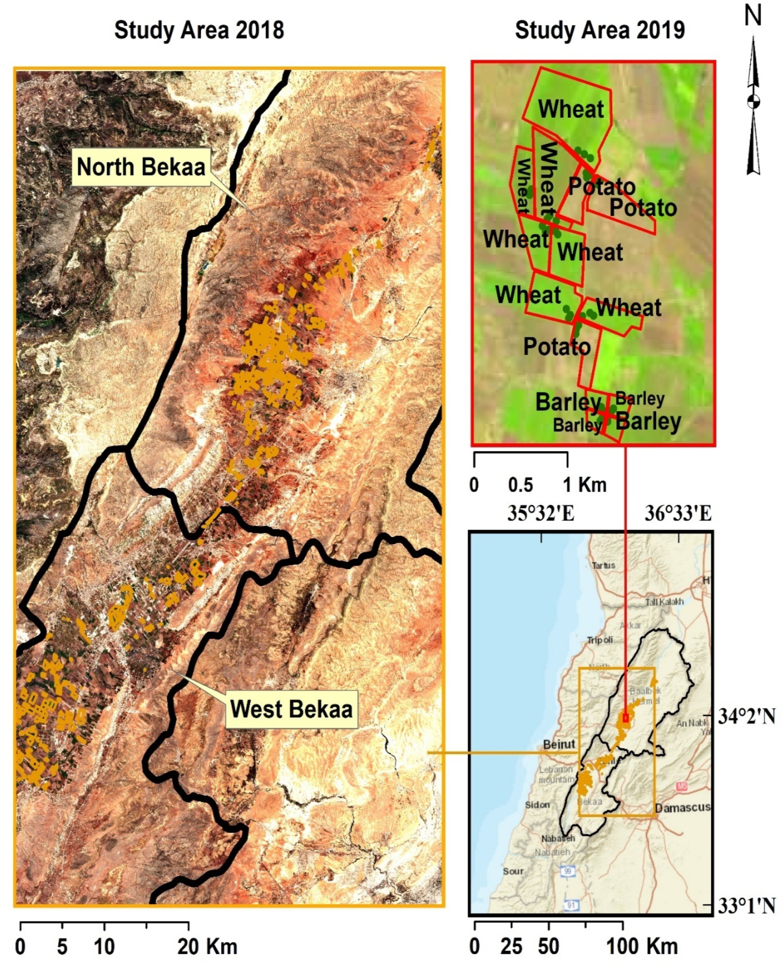
Figure 1.
Location of the study area within the Bekaa Valley. Fields surveyed during the 2018 field campaigns are outlined in light orange, while fields surveyed in 2019 are outlined in red. LAI, canopy height, and above-ground biomass sampling sites (labeled in dark green) for the 2019 growing season, the color version of the study area map is available online.
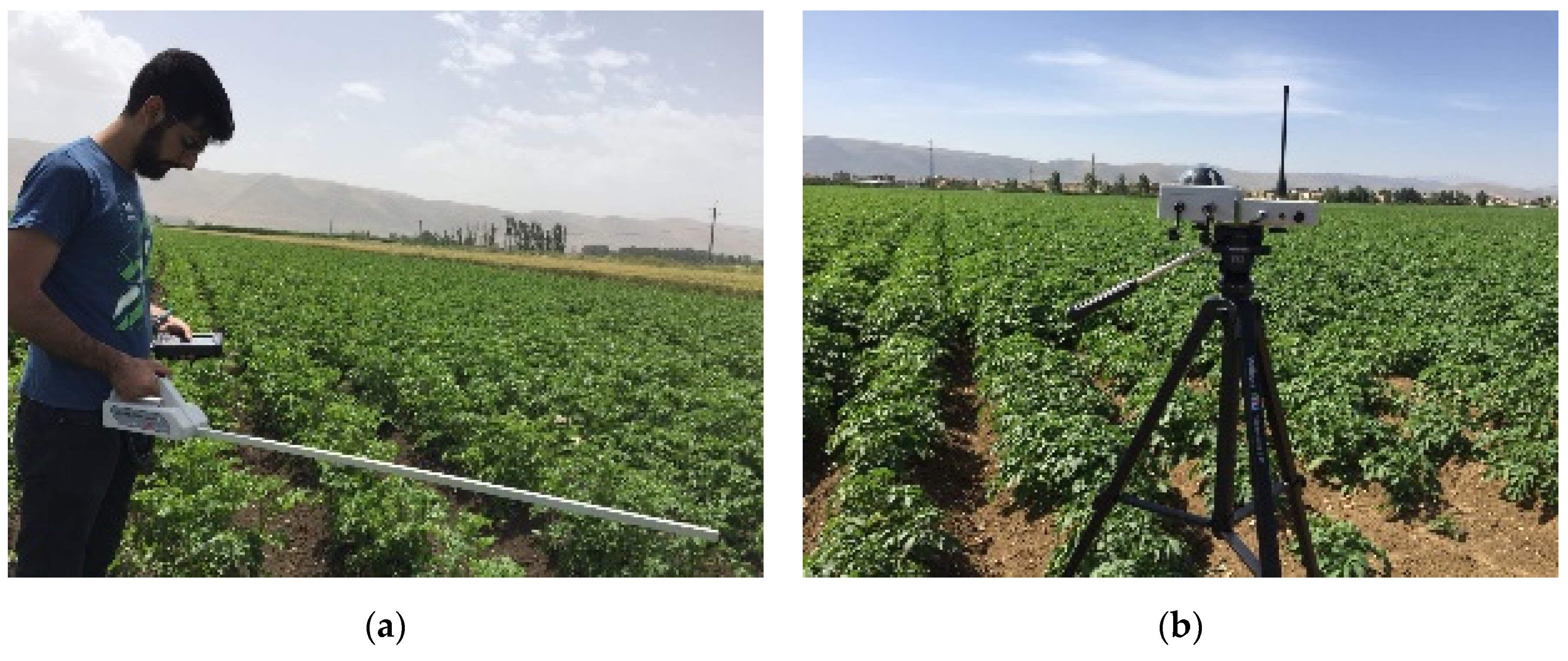
Figure 2.
LAI Measurements: (a) Data inputs to the SS1 SunScan Canopy Analysis System, (b) beam fraction sensor (BFS) installed in a potato field.
Figure 2.
LAI Measurements: (a) Data inputs to the SS1 SunScan Canopy Analysis System, (b) beam fraction sensor (BFS) installed in a potato field.
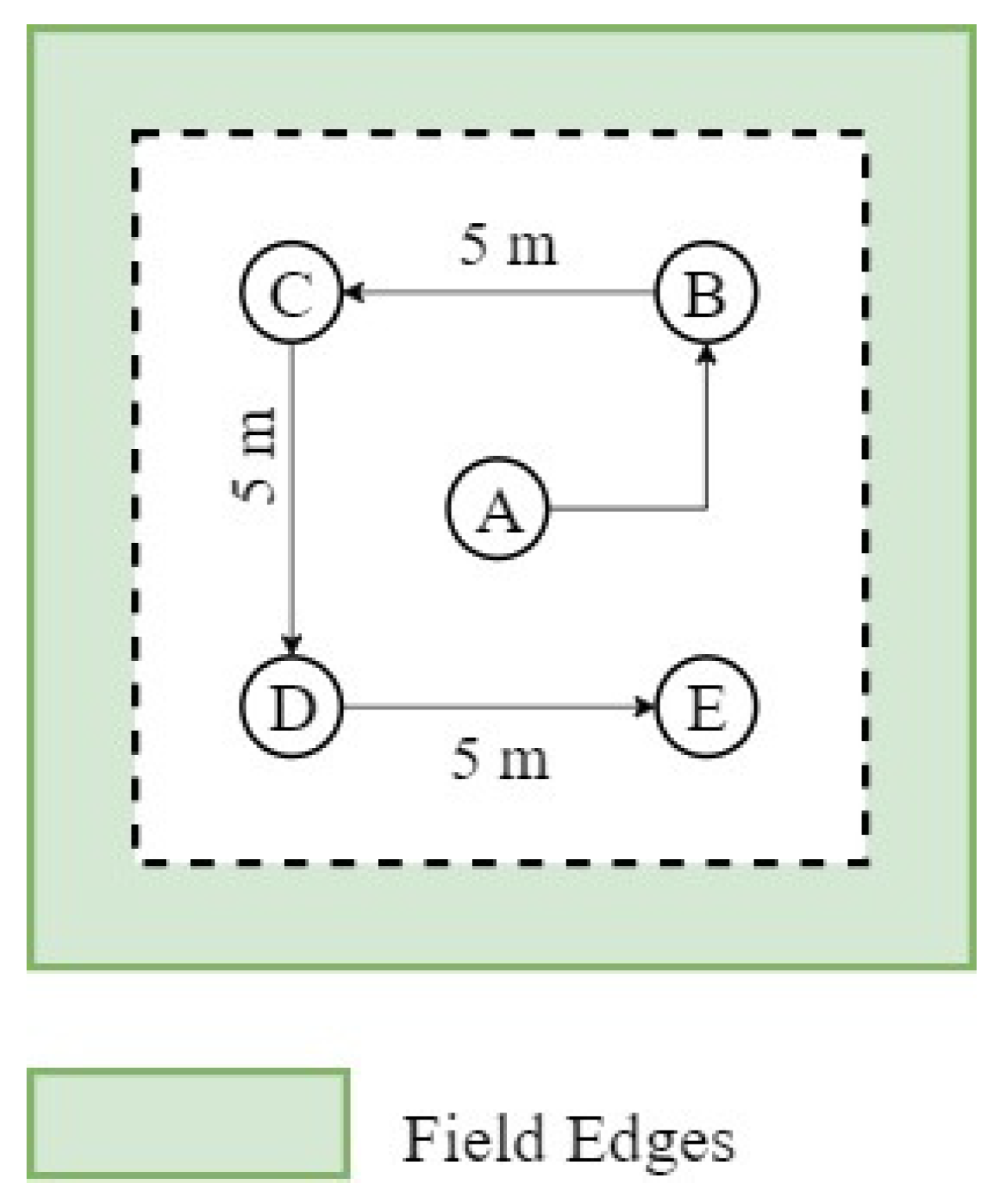
Figure 3.
LAI measurement approach for each visited field during 2018 growing season.
Figure 3.
LAI measurement approach for each visited field during 2018 growing season.
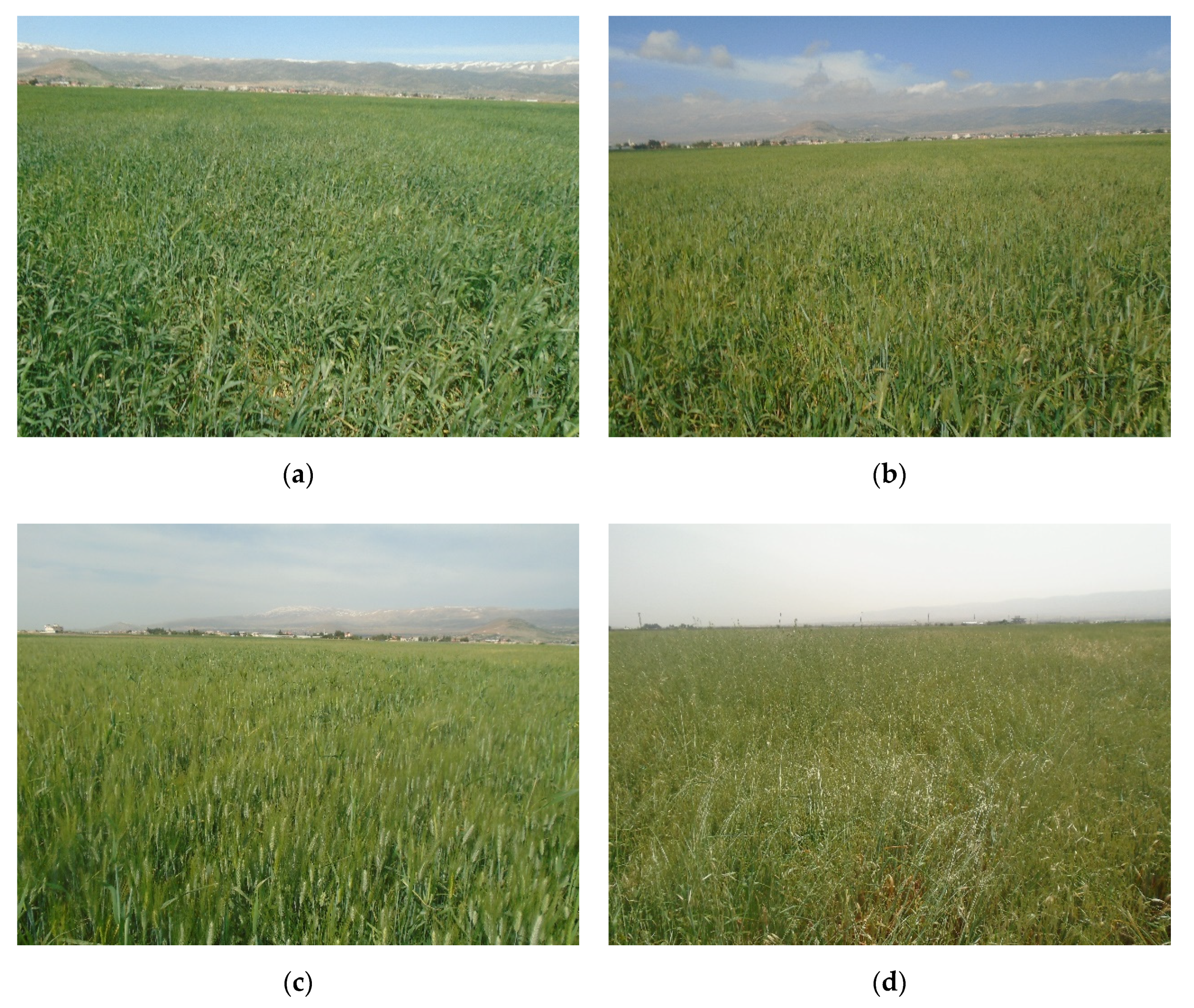
Figure 4.
Crop height and LAI field sampling at different growing stages of a wheat culture studied during the 2019 growing season: (a) DOY: 122, LAI: 2.3, height: 45 cm, (b) DOY: 131, LAI: 2.97, height: 73 cm, (c) DOY: 138, LAI: 3.03, height: 78 cm, (d) DOY: 141, LAI: 3.23, height: 58 cm.
Figure 4.
Crop height and LAI field sampling at different growing stages of a wheat culture studied during the 2019 growing season: (a) DOY: 122, LAI: 2.3, height: 45 cm, (b) DOY: 131, LAI: 2.97, height: 73 cm, (c) DOY: 138, LAI: 3.03, height: 78 cm, (d) DOY: 141, LAI: 3.23, height: 58 cm.
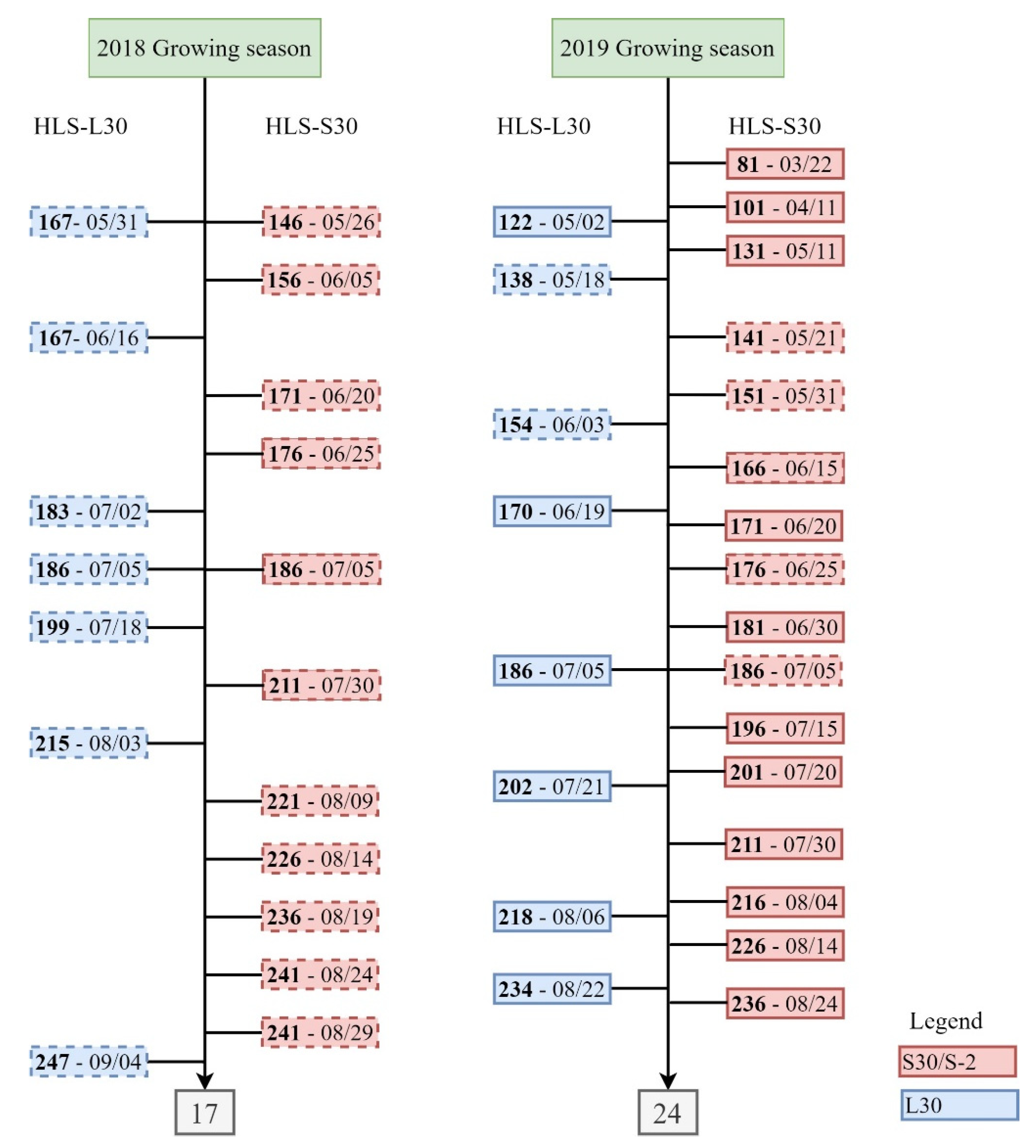
Figure 5.
Harmonized Landsat-8 and Sentinel-2 (HLS) scenes used in the study, showing the day of year (DOY) (in bold) with the respective date of HLS products (Landsat 8 (L30) images blue boxes, Sentinel-2 (S30) red boxes), with the respective number of total images in grey boxes. S2 images from THEIA were also obtained on the S2 dates (red boxes). Dashed boxes represent the HLS scenes used to validate LAI, whereas full boxes indicate scenes used to generate crop biophysical variable time-series during the 2019 growing season.
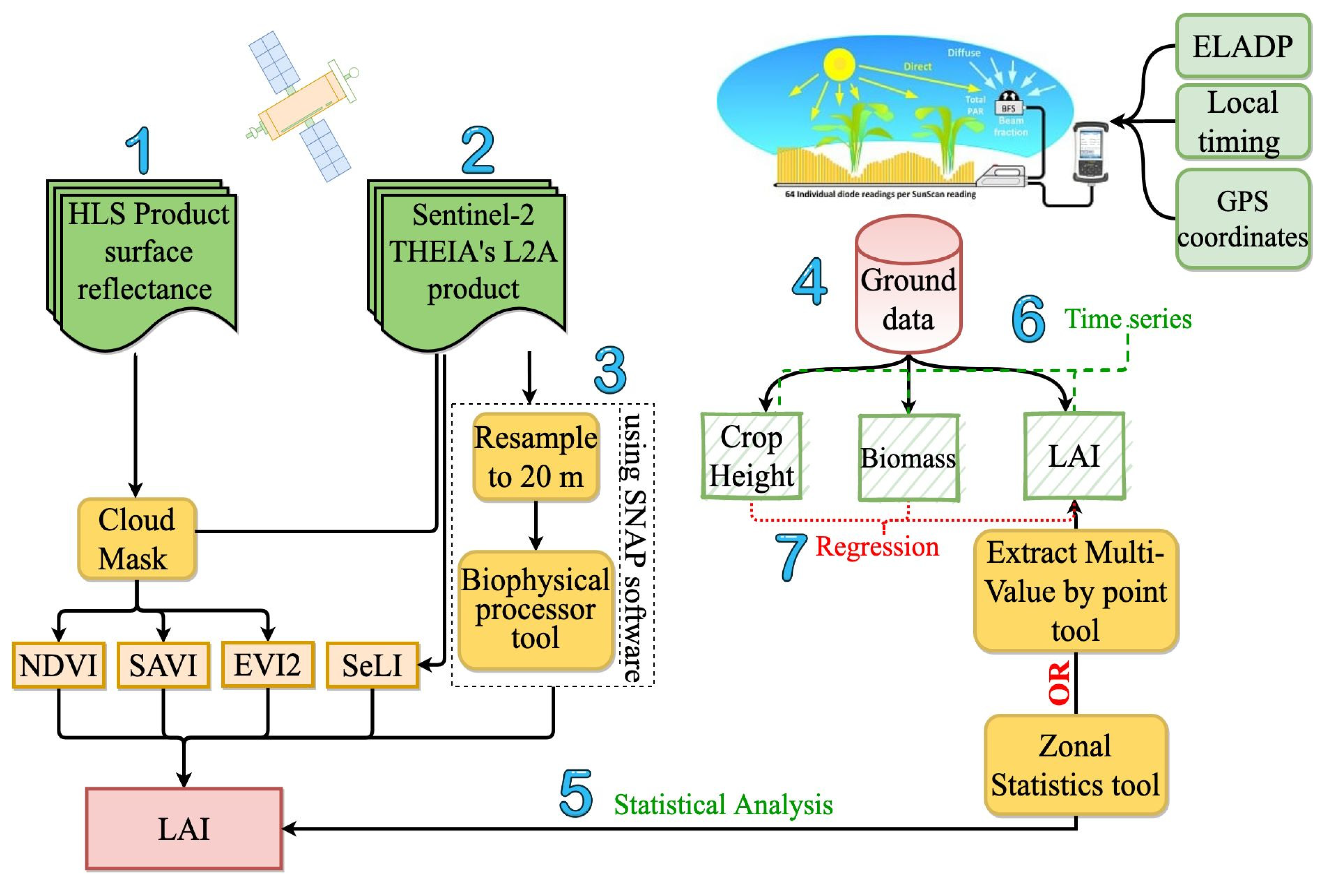
Figure 6.
Step-by-step flow chart for the validation of satellite-derived LAI against the ground measured LAI. Components of the analysis include: (1) existing vegetation index (VI) relationships applied to Harmonized Landsat-8 and Sentinel-2 (HLS) surface reflectance generated by NASA, (2) THEIA L2A surface reflectance products from Sentinel-2, (3) the SNAP biophysical model, (4) ground-truthing, (5) statistical comparison between the measured and the modeled LAI, (6) monitoring crop biophysical parameters during the 2019 growing season, and (7) investigation of crop-specific height and above-ground biomass relationships with LAI.
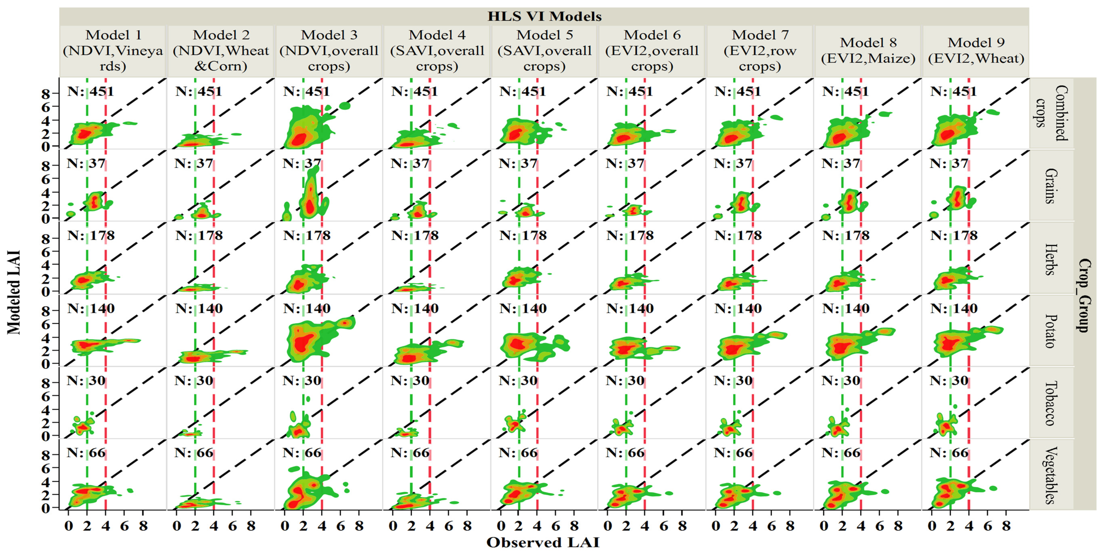
Figure 7.
Comparison between modeled and observed LAI in the 2018–2019 growing seasons for the HLS-VI models. The dashed green vertical lines represent the low observed LAI interval (0–2 m2/m2), the dashed red vertical lines represent the high observed LAI interval (>4 m2/m2), and the region between these two vertical lines represents the medium observed LAI range (2–4 m2/m2), the 2-D density plots represent four color levels with a dark red color at high density to dark green at lower densities, in addition to the orange and light green in representing medium densities.
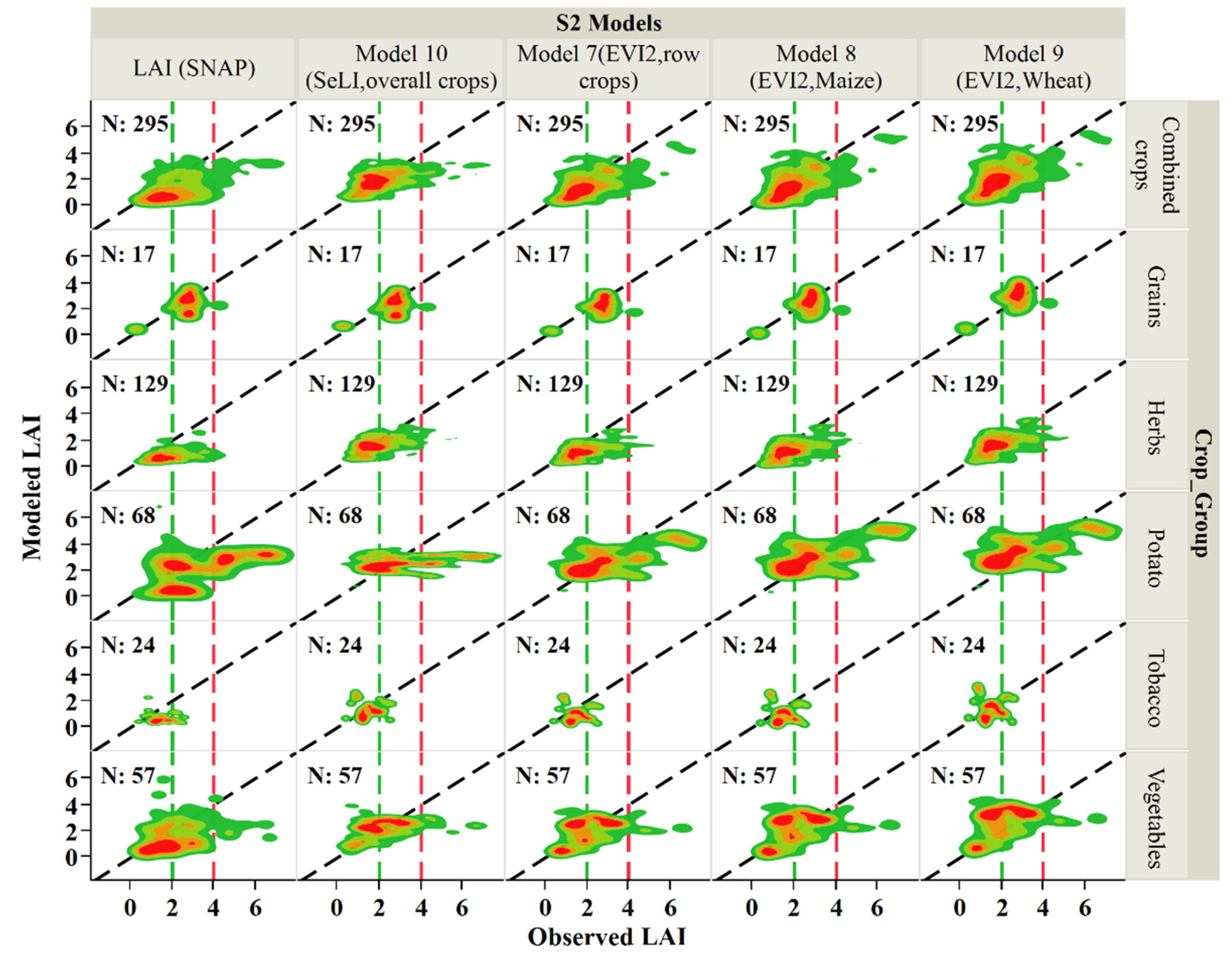
Figure 8.
Comparison between modeled and observed LAI in the 2018–2019 growing seasons for the HLS-VI for the HLS VI best-performing models derived from S30, Model 10 (SeLI, overall crops) and SNAP model derived from S2 THEIA product. The dashed green vertical lines represent the low observed LAI interval (0–2 m2/m2), the dashed red vertical lines represent the high observed LAI interval (>4 m2/m2), and the region between these two vertical lines represents the medium observed LAI range (2–4 m2/m2), the 2-D density plots represent four color levels with a dark red color at high density to dark green at lower densities, in addition to the orange and light green in representing medium densities.
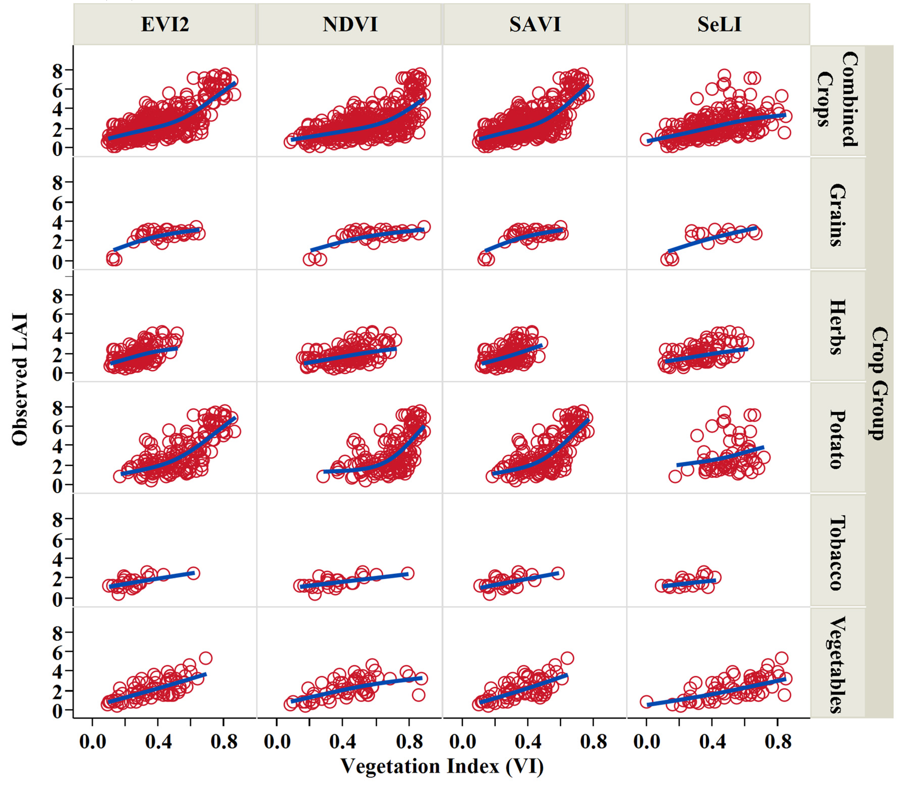
Figure 9.
Measured LAI as a function of vegetation indices (VI) derived from HLS product for the different studied crop groups and all crops combined.
Figure 9.
Measured LAI as a function of vegetation indices (VI) derived from HLS product for the different studied crop groups and all crops combined.
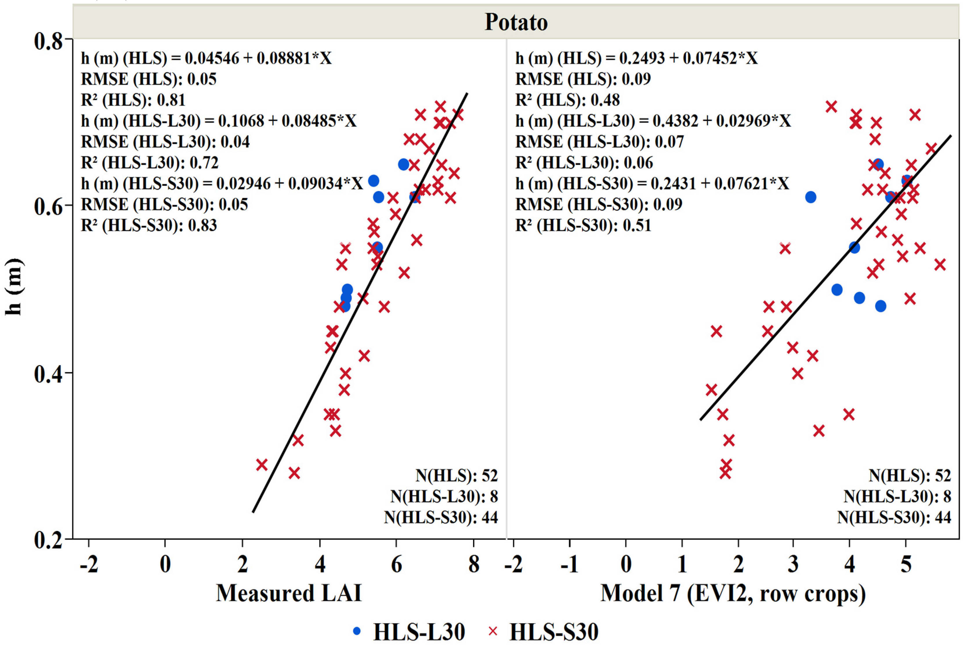
Figure 10.
Crop height (h (m)) as a function of measured LAI (m2/m2) and LAI derived from Model 7 (EVI2, row crops) for potato crop studied during the 2019 growing season. Blue points represent the measurements during Landsat overpass and the red crosses represent the measurements during Sentinel 2 overpass.
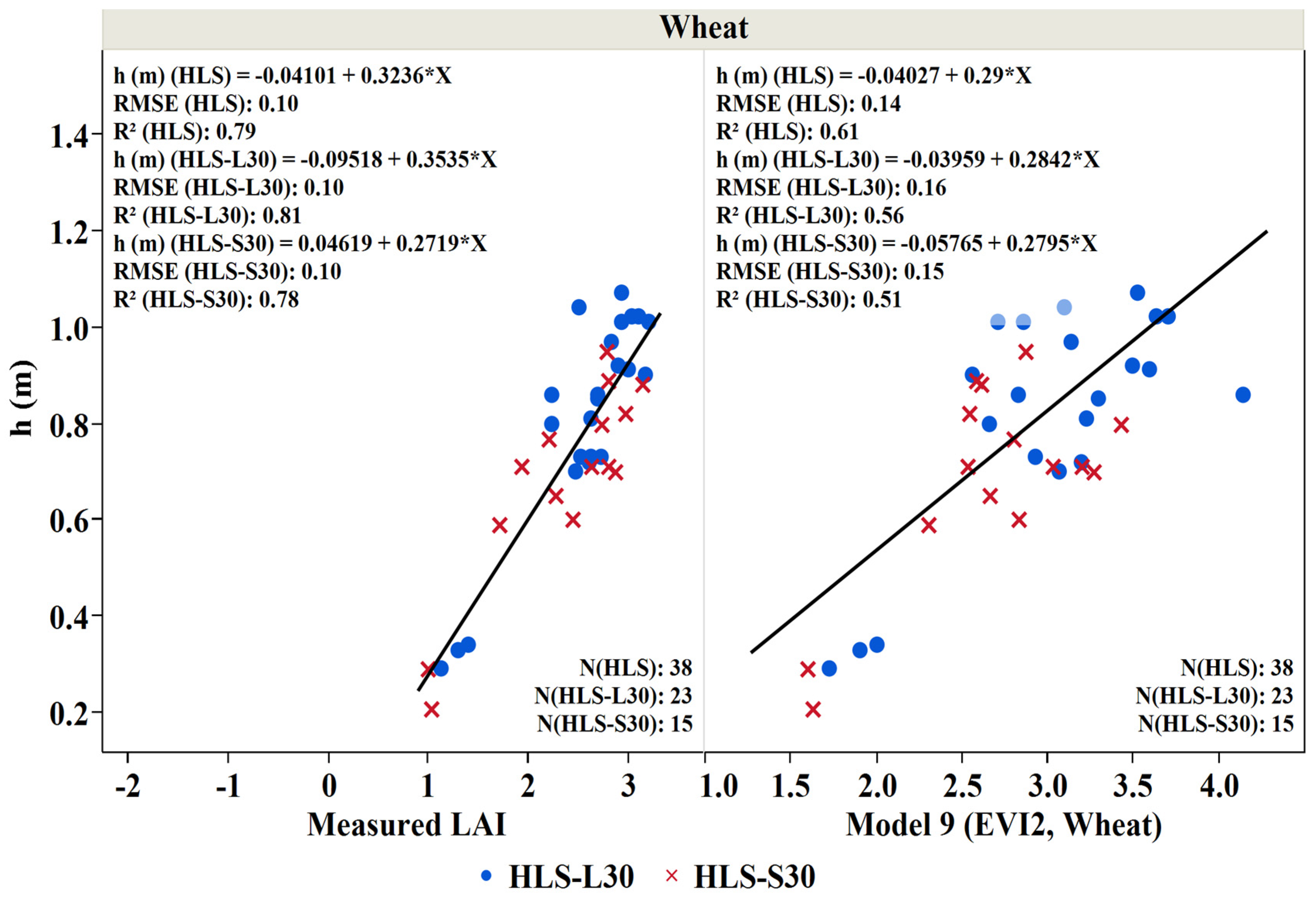
Figure 11.
Crop height (h (m)) as a function of measured LAI (m2/m2) and LAI derived from Model 9 (EVI2, wheat) for wheat crop studied during the 2019 growing season. Blue points represent the measurements during Landsat overpass and the red crosses represent the measurements during Sentinel 2 overpass.
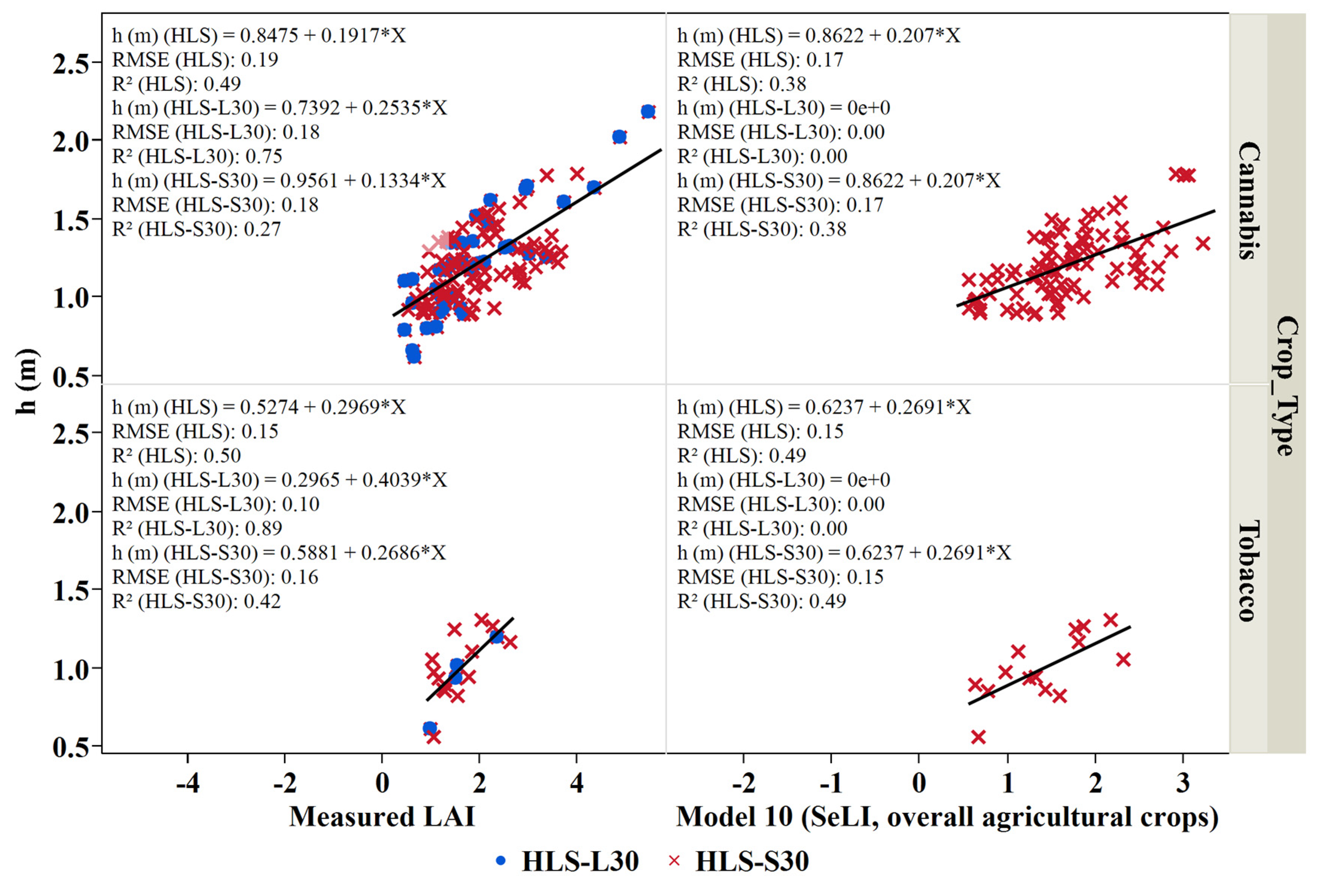
Figure 12.
Crop height (h (m)) as a function of measured LAI (m2/m2) and LAI derived from Model 10 (SeLI, overall agricultural crops) for cannabis and tobacco crops studied during the 2018 growing season. Blue points represent the measurements during Landsat overpass and the red crosses represent the measurements during Sentinel 2 overpass.
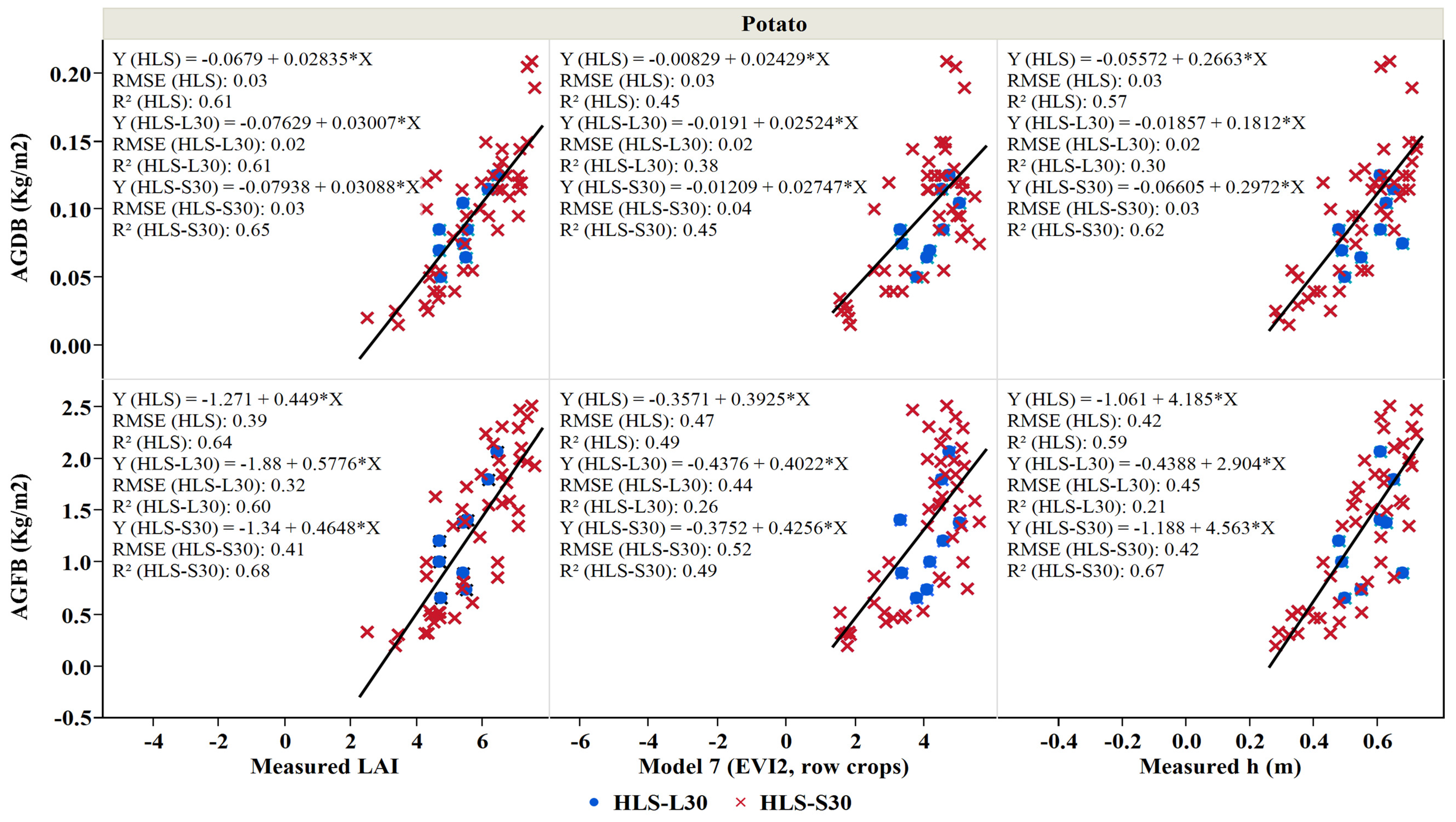
Figure 13.
Above-ground fresh (AGFB) and dry (AGDB) biomass weight as a function of LAI derived from Model 7 (EVI2, row crops), measured LAI, and height (h) for potato fields combined during the 2019 growing season. Blue points represent the measurements during Landsat overpass and the red crosses represent the measurements during Sentinel 2 overpass.
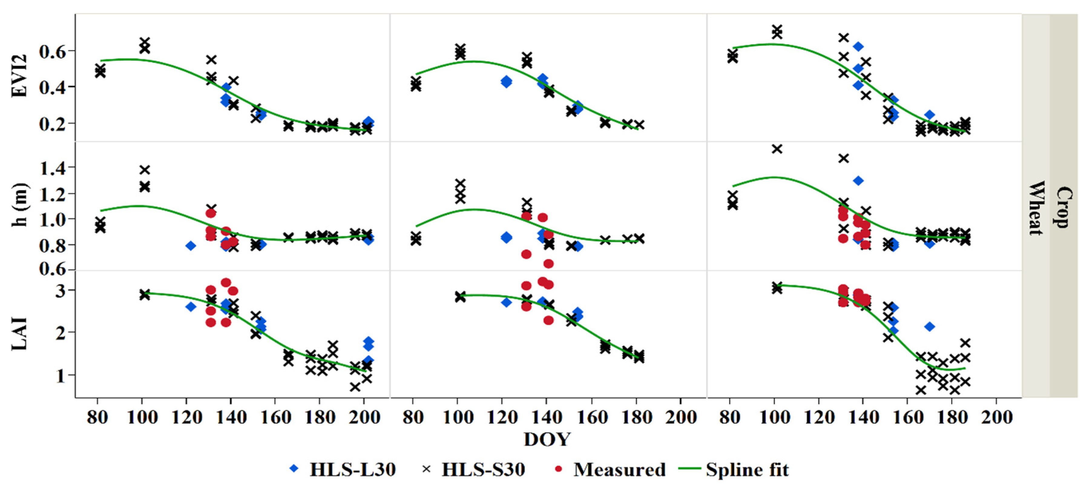
Figure 14.
A combined L30 and S30 derived and measured biophysical parameters (EVI2, h, and LAI) time-series of wheat for three farms during the 2019 growing season, modeled (both L30 and S30) crop biophysical in green spline fit.
Figure 14.
A combined L30 and S30 derived and measured biophysical parameters (EVI2, h, and LAI) time-series of wheat for three farms during the 2019 growing season, modeled (both L30 and S30) crop biophysical in green spline fit.
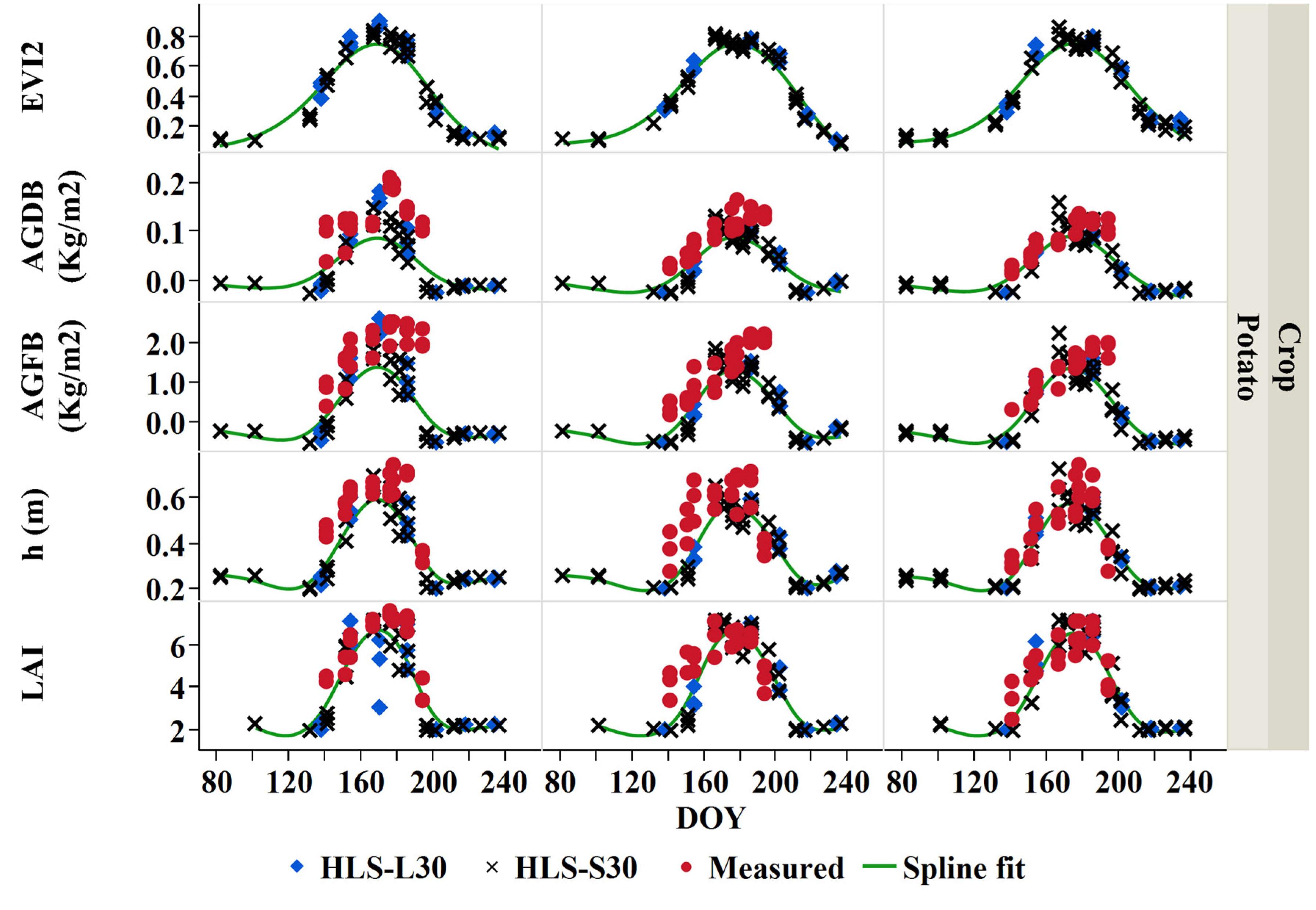
Figure 15.
A combined L30 and S30 derived and measured biophysical parameters (EVI2, above-ground fresh biomass (AGFB), above-ground dry biomass (AGDB), height (h), and leaf area index (LAI) time-series of potato for three farms during the 2019 growing season, modeled (both L30 and S30) crop biophysical in green spline fit.
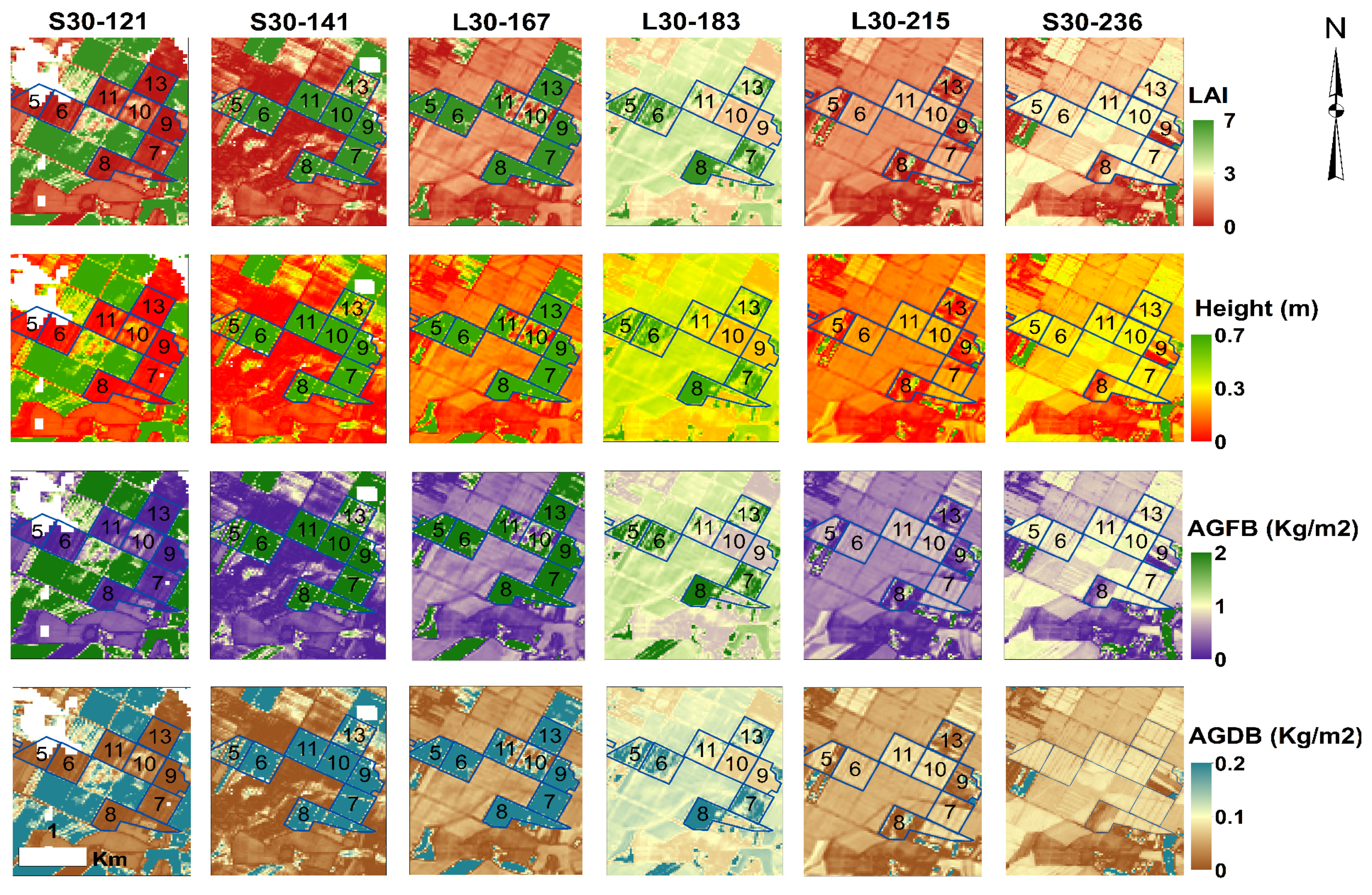
Figure 16.
Spatial and temporal biophysical parameter maps for different satellite (L30 and S30) overpass dates (DOY). The blue delineations indicate the surveyed potato fields during the 2018 season with their corresponding field IDs.
Figure 16.
Spatial and temporal biophysical parameter maps for different satellite (L30 and S30) overpass dates (DOY). The blue delineations indicate the surveyed potato fields during the 2018 season with their corresponding field IDs.
Table 1.
Surveyed crop groups during the 2018–2019 growing seasons, the number of fields and their average areas.
Table 1.
Surveyed crop groups during the 2018–2019 growing seasons, the number of fields and their average areas.
| Crop Group | Average Field Area (ha) | Number of Fields | Number of Leaf Area Index Measurements |
|---|
| Herbs | 9.3 | 178 | 890 |
| (Cannabis: Cannabis sativa, |
| Mint: Mentha, |
| Parsley: Petroselinum crispum) |
| Potato (Solanum tuberosum) | 12.4 | 140 | 700 |
| Tobacco (Nicotiana tabacum) | 5.1 | 30 | 150 |
| Vegetables | 7.3 | 66 | 330 |
| (Bean: Phaseolus vulgaris, |
| Cabbage: Brassica oleracea, |
| Carrot: Daucus carota subsp. sativus, |
| Chickpea: Cicer arietinum, |
| Corn: Zea mays, |
| Cucumber: Cucumis sativus, |
| Lettuce: Lactuca sativa, |
| Eggplant: Solanum melongena, |
| Melon: Cucumis melo var. cantalupensis, |
| Onion: Allium cepa |
| and Pepper: Capsicum annuum) |
| Grains | 9.9 | 37 | 185 |
| (Barley: Hordeum vulgare |
| and Wheat: Triticum aestivum) |
| All Crops | 9.6 | 451 | 2255 |
Table 2.
References and equations of selected VIs to be evaluated in this study.
Table 2.
References and equations of selected VIs to be evaluated in this study.
| Index | Acronym | Equation | Reference |
|---|
| Soil adjusted vegetation index | SAVI | | Huete [21] |
| Normalized difference vegetation index | NDVI | | Rouse Jr., et al. [61] |
| Enhanced vegetation index 2 | EVI2 | | Jiang et al. [23] |
| Sentinel-2 LAI | SeLI | | Pasqualotto et al. [30] |
Table 3.
A summary of the equations for the selected existing vegetation index-based LAI models evaluated in this study, along with the satellite and reflectance type used in the cited references.
Table 3.
A summary of the equations for the selected existing vegetation index-based LAI models evaluated in this study, along with the satellite and reflectance type used in the cited references.
| Model # | Relation | Equation of LAI | Studied Crop | Satellite and Reflectance | Reference |
|---|
| 1 | LAI-NDVI | 4.9NDVI − 0.46 | Vineyard | Multi-spectral imagery obtained from IKONOS, TOA reflectance | Johnson et al. [62] |
| 2 | | Wheat and Corn | Surface Reflectance L5 TM | González Piqueras [63] |
| 3 | | Overall vegetation cover and crops | Surface Reflectance, L5 TM | Myneni et al. [64] |
| 4 | LAI-SAVI | | Overall vegetation cover, woody trees, and agricultural crops | L5 TM and L7 ETM+, TOA reflectance | Pôçaset al. [65] |
| 5 | |
| 6 | LAI-EVI2 | | Overall crops | Surface Reflectance of L5 TM and L7 ETM+ | Kang et al. [58] |
| 7 | 0.58)2 | Row crops |
| 8 | | Maize |
| 9 | | Wheat |
| 10 | SeLI (Sentinel-2 LAI index) | 5.405 × SeLI − 0.114 | Overall crops (potato, artichoke, squash, alfalfa, lettuce, wheat, pumpkin, and others) | Surface Reflectance Sentinel-2 | Pasqualotto et al. [30] |
Table 4.
Statistical analysis summary for the studied crops in both 2018 and 2019 growing seasons for the vegetation indices derived from the HLS product models.
Table 4.
Statistical analysis summary for the studied crops in both 2018 and 2019 growing seasons for the vegetation indices derived from the HLS product models.
| HLS VI Models |
|---|
| LAI Model | Statistical Parameter | Herbs | Potato | Tobacco | Vegetables | Grains | Combined Crops |
|---|
| (n = 178) | (n = 140) | (n = 30) | (n = 66) | (n = 37) | (n = 451) |
|---|
| Model 1 (NDVI, Vineyard) | MAE | 0.82 | 1.28 | 0.64 | 0.98 | 0.74 | 0.97 |
| RMSE | 1.19 | 1.60 | 0.83 | 1.32 | 0.94 | 1.31 |
| RRMSE | 55% | 55% | 54% | 59% | 37% | 55% |
| MAPE | 39% | 64% | 52% | 54% | 66% | 52% |
| MBE | −0.43 | −0.09 | −0.06 | −0.11 | −0.26 | −0.24 |
| d | 0.66 | 0.50 | 0.66 | 0.57 | 0.69 | 0.63 |
| Model 2 (NDVI, Wheat and Corn) | MAE | 1.76 | 1.87 | 1.21 | 1.65 | 1.88 | 1.76 |
| RMSE | 2.07 | 2.40 | 1.35 | 2.09 | 2.10 | 2.16 |
| RRMSE | 97% | 82% | 88% | 94% | 82% | 90% |
| MAPE | 80% | 59% | 76% | 71% | 72% | 71% |
| MBE | −1.74 | −1.81 | −1.21 | −1.60 | −1.86 | −1.72 |
| d | 0.45 | 0.50 | 0.39 | 0.47 | 0.40 | 0.48 |
| Model 3 (NDVI, Overall agricultural crops) | MAE | 1.01 | 1.56 | 1.03 | 1.25 | 1.41 | 1.25 |
| RMSE | 1.35 | 1.95 | 1.26 | 1.67 | 1.77 | 1.64 |
| RRMSE | 63% | 67% | 82% | 75% | 69% | 68% |
| MAPE | 48% | 95% | 75% | 75% | 73% | 70% |
| MBE | −0.66 | 1.99 | −0.34 | 0.12 | 0.09 | 0.05 |
| d | 0.74 | 0.70 | 0.75 | 0.59 | 0.51 | 0.71 |
| Model 4 (SAVI, Overall agricultural crops) | MAE | 1.75 | 1.58 | 1.16 | 1.50 | 1.72 | 1.62 |
| RMSE | 2.06 | 1.97 | 1.30 | 1.95 | 1.96 | 1.97 |
| RRMSE | 96% | 68% | 84% | 88% | 76% | 82% |
| MAPE | 80% | 55% | 75% | 66% | 70% | 69% |
| MBE | −1.75 | −1.39 | −1.12 | −1.41 | −1.70 | −1.54 |
| d | 0.47 | 0.60 | 0.47 | 0.48 | 0.47 | 0.54 |
| Model 5 (SAVI, Overall agricultural crops) | MAE | 0.82 | 1.68 | 0.69 | 1.02 | 1.82 | 1.19 |
| RMSE | 1.12 | 2.09 | 0.88 | 1.40 | 1.97 | 1.59 |
| RRMSE | 52% | 72% | 57% | 63% | 77% | 66% |
| MAPE | 43% | 80% | 80% | 60% | 117% | 64% |
| MBE | −0.13 | −0.05 | 0.34 | 0.09 | −1.58 | −0.16 |
| d | 0.63 | 0.39 | 0.52 | 0.55 | 0.31 | 0.52 |
| Model 6 (EVI2, Overall agricultural crops) | MAE | 0.94 | 1.55 | 0.72 | 1.00 | 1.59 | 1.18 |
| RMSE | 1.33 | 2.08 | 0.88 | 1.37 | 1.76 | 1.62 |
| RRMSE | 62% | 71% | 57% | 61% | 68% | 68% |
| MAPE | 39% | 63% | 53% | 51% | 81% | 53% |
| MBE | −1.46 | −0.61 | −0.77 | −0.38 | −1.47 | −0.71 |
| d | 0.54 | 0.35 | 0.53 | 0.58 | 0.42 | 0.49 |
| Model 7 (EVI2, row crops) | MAE | 0.96 | 1.14 | 0.77 | 1.01 | 0.84 | 1.00 |
| RMSE | 1.35 | 1.42 | 0.92 | 1.38 | 1.10 | 1.34 |
| RRMSE | 63% | 49% | 60% | 62% | 43% | 56% |
| MAPE | 41% | 57% | 55% | 52% | 52% | 49% |
| MBE | −0.85 | −0.12 | −0.38 | −0.37 | −0.52 | −0.5 |
| d | 0.59 | 0.72 | 0.52 | 0.59 | 0.66 | 0.70 |
| Model 8 (EVI2, Maize) | MAE | 0.94 | 1.15 | 0.80 | 1.02 | 0.85 | 1.00 |
| RMSE | 1.31 | 1.41 | 0.99 | 1.38 | 1.08 | 1.32 |
| RRMSE | 61% | 48% | 65% | 62% | 42% | 55% |
| MAPE | 42% | 64% | 58% | 57% | 51% | 53% |
| MBE | −0.78 | 0.16 | −0.33 | −0.21 | −0.35 | −0.34 |
| d | 0.59 | 0.76 | 0.52 | 0.62 | 0.68 | 0.73 |
| Model 9 (EVI2, Wheat) | MAE | 0.80 | 1.29 | 0.76 | 1.05 | 0.85 | 0.99 |
| RMSE | 1.12 | 1.56 | 0.99 | 1.40 | 1.03 | 1.30 |
| RRMSE | 52% | 44% | 65% | 63% | 40% | 54% |
| MAPE | 40% | 78% | 63% | 66% | 67% | 59% |
| MBE | −0.33 | 0.62 | 0.09 | 0.23 | 0.16 | 0.11 |
| d | 0.66 | 0.72 | 0.60 | 0.64 | 0.69 | 0.74 |
Table 5.
Statistical analysis summary for the studied crops in both 2018 and 2019 growing seasons for the HLS VI best-performing models derived from S30, Model 10 (SeLI, overall crops) and SNAP model derived from S2 THEIA products.
Table 5.
Statistical analysis summary for the studied crops in both 2018 and 2019 growing seasons for the HLS VI best-performing models derived from S30, Model 10 (SeLI, overall crops) and SNAP model derived from S2 THEIA products.
| S2 Models |
|---|
| LAI Model | Statistical Parameter | Herbs | Potato | Tobacco | Vegetables | Grains | Combined Crops |
|---|
| (n = 129) | (n = 68) | (n = 24) | (n = 57) | (n = 17) | (n = 295) |
|---|
| Model 10 (SeLI, THEIA S2, Overall agricultural and row crops) | MAE | 0.82 | 1.44 | 0.69 | 1.01 | 0.70 | 0.98 |
| RMSE | 1.21 | 1.85 | 0.86 | 1.40 | 0.89 | 1.38 |
| RRMSE | 55% | 56% | 59% | 59% | 35% | 59% |
| MAPE | 36% | 52% | 58% | 55% | 51% | 46% |
| MBE | −0.49 | −0.69 | −0.11 | −0.19 | −0.36 | −0.44 |
| d | 0.56 | 0.43 | 0.42 | 0.51 | 0.73 | 0.58 |
| LAI-SNAP (THEIA S2) | MAE | 1.24 | 1.80 | 0.93 | 1.28 | 0.65 | 1.32 |
| RMSE | 1.61 | 2.19 | 1.08 | 1.73 | 0.83 | 1.72 |
| RRMSE | 73% | 66% | 73% | 73% | 33% | 70% |
| MAPE | 52% | 63% | 61% | 59% | 37% | 56% |
| MBE | −1.21 | −0.98 | −0.75 | −0.60 | −0.27 | −0.95 |
| d | 0.54 | 0.50 | 0.37 | 0.52 | 0.78 | 0.59 |
| Model 7 (EVI2, HLS VI, row crops) | MAE | 1.00 | 1.17 | 0.83 | 1.10 | 0.65 | 1.02 |
| RMSE | 1.39 | 1.50 | 0.98 | 1.46 | 0.91 | 1.38 |
| RRMSE | 63% | 45% | 66% | 62% | 36% | 57% |
| MAPE | 41% | 46% | 62% | 55% | 31% | 46% |
| MBE | −0.91 | −0.43 | −0.43 | −0.37 | −0.47 | −0.63 |
| d | 0.56 | 0.70 | 0.37 | 0.55 | 0.75 | 0.69 |
| Model 9 (EVI2, HLS VI, Wheat) | MAE | 0.79 | 1.21 | 0.78 | 1.14 | 0.70 | 0.95 |
| RMSE | 1.14 | 1.47 | 1.02 | 1.49 | 0.83 | 1.27 |
| RRMSE | 52% | 37% | 69% | 63% | 33% | 52% |
| MAPE | 36% | 60% | 70% | 68% | 44% | 51% |
| MBE | −0.40 | 0.32 | 0.003 | 0.26 | 0.21 | −0.04 |
| d | 0.64 | 0.73 | 0.40 | 0.60 | 0.79 | 0.74 |
| Model 8 (EVI2, HLS VI, Maize) | MAE | 0.97 | 1.12 | 0.86 | 1.11 | 0.64 | 1.01 |
| RMSE | 1.35 | 1.40 | 1.04 | 1.47 | 0.87 | 1.34 |
| RRMSE | 62% | 42% | 71% | 62% | 35% | 55% |
| MAPE | 42% | 50% | 65% | 60% | 27% | 48% |
| MBE | −0.85 | −0.12 | −0.41 | −0.18 | −0.30 | −0.48 |
| d | 0.60 | 0.76 | 0.37 | 0.57 | 0.79 | 0.73 |
Table 6.
Statistics obtained using regression equations of the form y = (a × VI + b) × (1 + c × exp (d × VI)) for each of the studied index, for the studied crop groups.
Table 6.
Statistics obtained using regression equations of the form y = (a × VI + b) × (1 + c × exp (d × VI)) for each of the studied index, for the studied crop groups.
| Crop Group | VI | Regression Coefficients | | p-Value | RMSE | R2 |
|---|
| | a | b | c | d | | | |
|---|
| Grains (n = 36) | EVI2 | 4.5 | −0.6 | 15.0 | −6.23 | <0.0001 | 0.34 | 0.82 |
| SAVI | −0.02 | 2.9 | −5.5 | −12.57 | <0.0001 | 0.34 | 0.81 |
| NDVI | −0.3 | 3.1 | −5.4 | −7.93 | <0.0001 | 0.37 | 0.78 |
| SeLI | −0.4 | 3.0 | −4.8 | −11.47 | 0.001 | 0.43 | 0.77 |
| Potato (n = 158) | EVI2 | −2.7 | 2.5 | 0.009 | 9.63 | <0.0001 | 1.25 | 0.59 |
| SAVI | −3.4 | 2.7 | 0.003 | 12.36 | <0.0001 | 1.25 | 0.59 |
| NDVI | −3.8 | 3.7 | 0.0001 | 14.10 | <0.0001 | 1.35 | 0.52 |
| SeLI | 0.01 | 0.004 | 306.3 | 0.00 | 0.03 | 1.59 | 0.06 |
| Herbs (n = 136) | EVI2 | −1.1 | 0.8 | 0.3 | 7.34 | <0.0001 | 0.69 | 0.34 |
| SAVI | 1.1 | 0.2 | 1.6 | 1.30 | <0.0001 | 0.74 | 0.23 |
| NDVI | 1.6 | 2.4 | −0.9 | −1.67 | <0.0001 | 0.73 | 0.29 |
| SeLI | 1.0 | 0.3 | 1.3 | 1.12 | <0.0001 | 0.69 | 0.32 |
| Tobacco (n = 25) | EVI2 | 0.01 | 0.0020 | 383.4 | 0.00 | 0.00036 | 0.40 | 0.43 |
| SAVI | 0.01 | 0.0022 | 347.7 | 0.00 | 0.00116 | 0.43 | 0.37 |
| NDVI | 0.01 | 0.0020 | 302.0 | 0.00 | <0.0001 | 0.37 | 0.49 |
| SeLI | 0.01 | 0.0022 | 369.9 | 0.00 | 0.006 | 0.35 | 0.39 |
| Vegetables (n = 70) | EVI2 | 4.0 | 0.5 | 0.0007 | 9.39 | <0.0001 | 0.74 | 0.53 |
| SAVI | 0.02 | 0.004 | 143.9 | 0.88 | <0.0001 | 0.79 | 0.47 |
| NDVI | 0.1 | 0.022 | 20.8 | 0.21 | <0.0001 | 0.85 | 0.38 |
| SeLI | 0.0002 | 0.000 | 19,210.5 | 0.00 | <0.0001 | 0.90 | 0.35 |
| All Crops (n = 425) | EVI2 | 2.9 | 0.8 | 0.01 | 5.46 | <0.0001 | 0.94 | 0.63 |
| SAVI | 3.2 | 0.7 | 0.003 | 7.93 | <0.0001 | 0.97 | 0.61 |
| NDVI | 1.0 | 1.1 | 0.01 | 5.72 | <0.0001 | 1.07 | 0.51 |
| SeLI | 1.1 | 0.032 | 4.94 | −0.56 | <0.0001 | 1.10 | 0.27 |
Table 7.
Regression coefficients obtained by regressing LAI against EVI2 using the equation of the form y = (a × VI + b) × (1 + c × exp (d × VI)), for the studied crop groups, separated by satellite type, L30, and S30.
Table 7.
Regression coefficients obtained by regressing LAI against EVI2 using the equation of the form y = (a × VI + b) × (1 + c × exp (d × VI)), for the studied crop groups, separated by satellite type, L30, and S30.
| Crop Group | VI | L30 | S30 |
|---|
| Regression Coefficients | Regression Coefficients |
|---|
| a | b | c | d | a | b | c | d |
|---|
| Grains | EVI2 | 0.00 | 0.01 | 123.21 | 0.26 | 1.28 | 0.30 | 1.57 | 0.47 |
| Potato | −1.81 | 1.61 | 0.01 | 10.36 | −3.56 | 3.26 | 0.00 | 10.41 |
| Herbs | 7.52 | −0.51 | 0.00 | 0.00 | 4.98 | 0.47 | 0.00 | 0.00 |
| Tobacco | 4.13 | 0.37 | 0.00 | 0.00 | 3.08 | 0.91 | 0.00 | 0.00 |
| Vegetables | 4.34 | 0.22 | 0.01 | 6.77 | 4.04 | 0.50 | 0.00 | 9.39 |
| Combined Crops | 4.07 | 0.35 | 0.00 | 7.93 | 1.34 | 0.99 | 0.11 | 3.63 |
Table 8.
Statistical comparison between modeled and observed LAI separated by satellite type: L30, S30, and L30 and S30 combined, the modeled LAI is obtained using the LAI-EVI2 empirical relationships displayed in
Table 6.
Table 8.
Statistical comparison between modeled and observed LAI separated by satellite type: L30, S30, and L30 and S30 combined, the modeled LAI is obtained using the LAI-EVI2 empirical relationships displayed in
Table 6.
| Crop Group | Statistical Parameter | L30 | S30 | L30 and S30 |
|---|
| Grains (n = 36) | RMSE | 1.46 | 0.60 | 0.32 |
| MAE | 1.41 | 0.48 | 0.25 |
| Potato (n = 158) | RMSE | 1.30 | 1.23 | 1.20 |
| MAE | 0.99 | 0.99 | 0.94 |
| Herbs (n = 136) | RMSE | 0.76 | 0.71 | 0.69 |
| MAE | 0.61 | 0.58 | 0.55 |
| Tobacco (n = 25) | RMSE | 0.46 | 0.41 | 0.40 |
| MAE | 0.37 | 0.32 | 0.31 |
| Vegetables (n = 70) | RMSE | 0.74 | 0.71 | 0.71 |
| MAE | 0.58 | 0.59 | 0.59 |
| Combined Crops (n = 425) | RMSE | 1.05 | 0.92 | 0.89 |
| MAE | 0.80 | 0.71 | 0.66 |
Table 9.
Statistical comparison between modeled and observed height (h(m)) separated by satellite type: L30, S30, and L30 and S30 combined, modeled height is obtained from equations displayed in
Figure 10,
Figure 11 and
Figure 12 as a function of observed LAI.
Table 9.
Statistical comparison between modeled and observed height (h(m)) separated by satellite type: L30, S30, and L30 and S30 combined, modeled height is obtained from equations displayed in
Figure 10,
Figure 11 and
Figure 12 as a function of observed LAI.
| Crop Group | Statistical Parameter | L30 | S30 | L30 and S30 |
|---|
| Wheat | RMSE | 0.104 | 0.113 | 0.101 |
| (n = 38) | MAE | 0.085 | 0.092 | 0.084 |
| Potato | RMSE | 0.065 | 0.053 | 0.052 |
| (n = 52) | MAE | 0.051 | 0.045 | 0.044 |
| Cannabis | RMSE | 0.194 | 0.193 | 0.185 |
| (n = 128) | MAE | 0.163 | 0.161 | 0.157 |
| Tobacco | RMSE | 0.167 | 0.146 | 0.145 |
| (n = 18) | MAE | 0.135 | 0.118 | 0.116 |
Table 10.
Statistical comparison between modeled and observed above-ground dry biomass (AGDB) and above-ground fresh biomass (AGFB) for potato separated by satellite type: L30, S30, and L30 and S30 combined, modeled fresh and dry above-ground biomass is obtained from equations displayed in
Figure 13 as a function of observed LAI.
| Biophysical Parameter | Statistical Parameter | L30 | S30 | L30 and S30 |
|---|
| Potato AGDB | RMSE | 0.026 | 0.026 | 0.026 |
| (n = 146) | MAE | 0.020 | 0.020 | 0.020 |
| RRMSE | 29% | 29% | 29% |
| Potato AGFB | RMSE | 0.424 | 0.390 | 0.390 |
| (n = 146) | MAE | 0.348 | 0.337 | 0.338 |
| RRMSE | 35% | 32% | 32% |


