Joint Use of Spaceborne Microwave Sensor Data and CYGNSS Data to Observe Tropical Cyclones


1
School of Electronic Information, Wuhan University, Wuhan 430072, China
2
School of Remote Sensing and Information Engineering, Wuhan University, Wuhan 430079, China
*
Author to whom correspondence should be addressed.
Remote Sens. 2020, 12(19), 3124; https://doi.org/10.3390/rs12193124
Submission received: 12 August 2020
/
Revised: 14 September 2020
/
Accepted: 21 September 2020
/
Published: 23 September 2020
(This article belongs to the Special Issue Advances of Remote Sensing in Environmental Geoscience)
Abstract
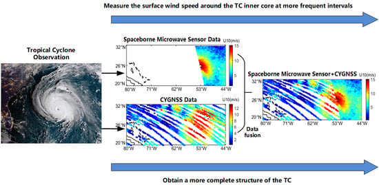
:The joint use of spaceborne microwave sensor data and Cyclone Global Navigation Satellite System (CYGNSS) data to observe tropical cyclones (TCs) is presented in this paper. The Soil Moisture Active and Passive (SMAP) radiometer was taken as an example of a spaceborne microwave sensor, and its data and the CYGNSS data were fused to fix the center of a TC and to measure the maximum wind speed around the TC inner core. This process included data preprocessing, image fusion, determination of the TC center position, and the estimation of the TC’s intensity. For all of the observed hurricanes, the experimental results demonstrated that the proposed method obtains a more complete structure of the TC and can measure the surface wind speed around the TC inner core at more frequent intervals compared to the case where the SMAP radiometer data or the CYGNSS data are employed alone. Furthermore, when comparing the TC tracks obtained by the proposed method with the best tracks provided by the National Hurricane Center (NHC), we found that the mean absolute error values ranged between 18.4 and 46 km, the standard deviation varied between 15.1 and 28.2 km, and both of these were smaller than the values obtained by only using the CYGNSS data. In addition, when comparing the maximum wind speed around the TC inner core obtained by the proposed method with the best track peak winds estimated by the NHC, we found that the mean absolute error values ranged between 7.7 and 15.7 m/s, the root-mean-square difference values varied between 8.6 and 18 m/s, the correlation coefficients varied between 0.1782 and 0.9877, the bias values varied between −8.5 and 4.5 m/s, and all of these values were smaller in most cases, than those obtained by only using the CYGNSS data.
1. Introduction
Tropical cyclones (TCs) cause disasters that lead to the loss of life and property in many parts of the world every year. To minimize the losses caused by TCs and to organize disaster mitigation measures, it is crucial that the center position of the TC is quickly and accurately determined and that it is monitored at frequent intervals [1]. Furthermore, the surface wind speed around the TC’s inner core and its minimum pressure should be measured to estimate its intensity.
Various satellite-borne sensors have been employed to routinely observe TCs such as visible and infrared imagers that are carried by geostationary meteorological satellites [2], microwave radiometers and scatterometers carried by polar orbiting satellites [3,4], and the synthetic aperture radar (SAR) carried by low-earth orbiting satellites [5]. Each has its own benefits and drawbacks. For example, the geostationary meteorological satellite has a high temporal resolution and a large imaging area, but it is unable to directly measure the ocean surface wind speed. In contrast, most spaceborne microwave sensors can measure the global ocean surface wind speed in all weather and time conditions. However, their performance is severely limited by the long revisit period, and this makes it difficult to obtain adequate samples during the rapidly evolving stages of a TC’s life cycle. In addition, the coverage of a microwave radiometer or scatterometer is not continuous because of the gap between its swaths. As a result, the complete structure of a TC cannot be obtained in some cases. For example, the inner core of Hurricane Florence was located outside the coverage of the Soil Moisture Active and Passive (SMAP) satellite at 08:30 Coordinated Universal Time (UTC) on 10 September 2018, as described in Section 3, and hence it is impossible to determine the location of Hurricane Florence by only using the SMAP satellite data. Therefore, the joint use of multiple satellite data to provide more information about TCs is very important to improve the accuracy of TC prediction [6].
The global navigation satellite system-reflectometry (GNSS-R) technique is a new application of satellite navigation systems that was first proposed by Martin-Neira in 1993 and it has attracted a lot of attention within the remote sensing community [7]. GNSS-R is a passive radar system that uses GNSS satellites as transmitters of opportunity, e.g., the Global Position System (GPS), GLONASS, Galileo, and Beidou. In recent years, the GNSS-R technique has been widely studied both at the theoretical and practical level. Various theoretical models have been proposed for GNSS-R [8,9]. In the meantime, numerous experiments have been conducted to evaluate the potential of GNSS-R in applications such as ocean altimetry [10], as well as the detection of sea ice, oil slicks, ocean surface wind fields, snow depth, soil moisture, and vegetation status [11]. In order to demonstrate the potential of spaceborne GNSS-R in monitoring the global environment, several satellites equipped with the GNSS-R payload were launched during the last two decades [12]. One of them is the National Aeronautics and Space Administration (NASA) Cyclone Global Navigation Satellite System (CYGNSS) that was launched on 15 December 2016. The CYGNSS constellation consists of eight low-earth orbiting microsatellites, and its scientific goal is to understand the relationship between ocean surface properties, moist atmospheric thermodynamics, radiation, and convective dynamics in the inner core of TCs [13]. Its primary objectives are to measure ocean surface wind speed in the range of 3–70 m/s with a spatial coverage between 35° N and 35° S latitude, a spatial resolution of 25 × 25 km, and a mean revisit time that is better than 12 h [14]. As a result, more information about TCs can be obtained, which enhances our understanding of their physical processes and helps to forecast their genesis and intensification.
After the launch of CYGNSS, many studies have reported on its data processing, as well as its potential in the observation of TCs. A calibration algorithm used by the CYGNSS mission to produce its Level 1 data products is described in [15]. A wind speed retrieval algorithm to obtain the CYGNSS Level 2 data products and its retrieval error was introduced in [16,17], respectively. In addition, several methods have been proposed to estimate the center location, intensity and integrated kinetic energy of TCs [18,19,20], and the performance of the GNSS constellation was studied at both a theoretical and practical level when it was employed to observe the ocean surface winds within the TC inner core [21,22,23,24,25,26,27,28]. These studies have shown that the assimilation of CYGNSS data can improve the prediction of TC position, intensity, and structure. Nevertheless, as shown in the latter sections of this paper, the tracks of the CYGNSS satellite are narrow and sometimes sparse, which makes it difficult to obtain the complete structure of a TC in order to fix its center and to estimate its intensity when only the CYGNSS data are used.
In this paper, the SMAP radiometer was taken as an example of spaceborne microwave sensor, and its data and the CYGNSS data were used together to obtain a more complete structure of TCs. The goal of this study was to measure the surface wind speed around the TC inner core at more frequent intervals compared to the case in which the SMAP radiometer data or the CYGNSS data are employed alone to observe TCs. This paper is organized as follows. A brief introduction to the observation data employed to monitor TCs is provided in Section 2. The SMAP radiometer data and the CYGNSS data were combined to estimate the center position and maximum wind speed of TCs, and the steps used to process the observation data are described in Section 3. The results are discussed in Section 4 and finally, the main conclusions are summarized in Section 5.
2. Observation Data
2.1. CYGNSS Data
The CYGNSS mission provides five levels of data products, and four of them are available to the public, i.e., Level 1 to 4 data products. The Level 2 data products consist of the mean square slope product and the ungridded wind speed product over a 25 km × 25 km region centered at the specular point. The Level 2 wind speed products are estimated by using the delay-Doppler map (DDM) average and leading-edge slope observables that are derived from the Level 1B DDMs of bistatic radar cross section and the DDMs of effective scattering area [29]. More details about the CYGNSS data products can be found in [29]. In this study, version 2.1 of CYGNSS Level 2 data products (downloaded from https://podaac-tools.jpl.nasa.gov/drive/files/allData/cygnss/L2/V2.1) were used to observe the TCs of interest.
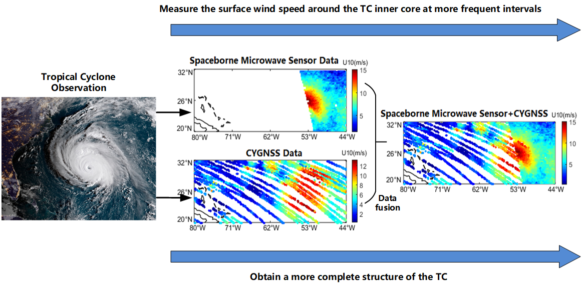
It is worth noting that since the relationship between surface roughness and wind speed is not unique under different sea state conditions, two geophysical model functions (GMFs) were used for the wind speed retrieval to obtain the CYGNSS Level 2 data products. One of them is the fully developed seas (FDS) model, which is suited for the general sea state condition, and the other is the young seas with limited fetch (YSLF) model, which is suited for the sea state near or in a TC. More details about the above two GMFs can be found in [30]. In this study, the Level 2 data products derived by the FDS GMF were used to analyze the central position of TCs because the wind products derived by the FDS GMF highlight the central position of TCs by contrasting low values near the center with surrounding higher values. However, the wind products derived by the FDS GMF were not used to estimate the wind speed around the inner core of TCs. This is because the FDS GMF is restricted at high wind speeds due to the limitations in the dynamic range of wind speeds included in the training dataset [30]. Therefore, we used the Level 2 data products derived by the YSLF GMF to estimate the 10-m-referenced ocean surface wind speed (U10) around the inner core of TCs. This is because the YSLF GMF is based on matchups between measurements made by CYGNSS and the stepped frequency microwave radiometer on hurricane hunter aircraft. These matchups show that the CYGNSS L1 observables are fairly and consistently sensitive to changes in high wind speeds. As a result, the YSLF GMF performs better in estimating wind speed around the inner core of TCs than the FDS GMF [30]. Wind speeds retrieved from version 2.1 of CYGNSS Level 2 data products on 10 September 2018 are shown in Figure 1.
2.2. SMAP Radiometer Data
The NASA SMAP mission, launched on 29 January 2015, is a combination of passive (radiometer operating at 1.41 GHz) and active (scatterometer operating at 1.26 GHz) L-band sensors designed to provide global soil moisture and freeze/thaw classification. It flies in a polar 8-day repeat orbit at an average altitude of 685 km and maps out a contiguous swath of about 1000-km in width. In addition, the spatial resolution of the SMAP radiometer is about 40 km. Although designed for hydrological applications over land surfaces, it also has excellent capabilities to measure ocean surface salinity and ocean winds in storms. The SMAP radiometer can measure wind speeds up to 65 m/s without being affected by rain [31]. Furthermore, for wind speeds in the range of 20–40 m/s, the difference in the root-mean-square of the wind speed retrieved from the SMAP radiometer data compared to the stepped frequency microwave radiometer (SFMR) observations is about 4.6 m/s [32]. More details about SMAP and its radiometer data can be found in [31].
In this study, version 4.3 of SMAP radiometer Level 2 data products (downloaded from https://podaac-tools.jpl.nasa.gov/drive/files/allData/smap/L2/JPL/V4.3), which includes the wind speed and direction for high winds, were adopted to observe the TCs of interest. Wind speeds retrieved from version 4.3 of SMAP radiometer Level 2 data products on 12 September 2018 are shown in Figure 2. A hurricane can be observed in the top right portion of this figure.
3. Data Processing
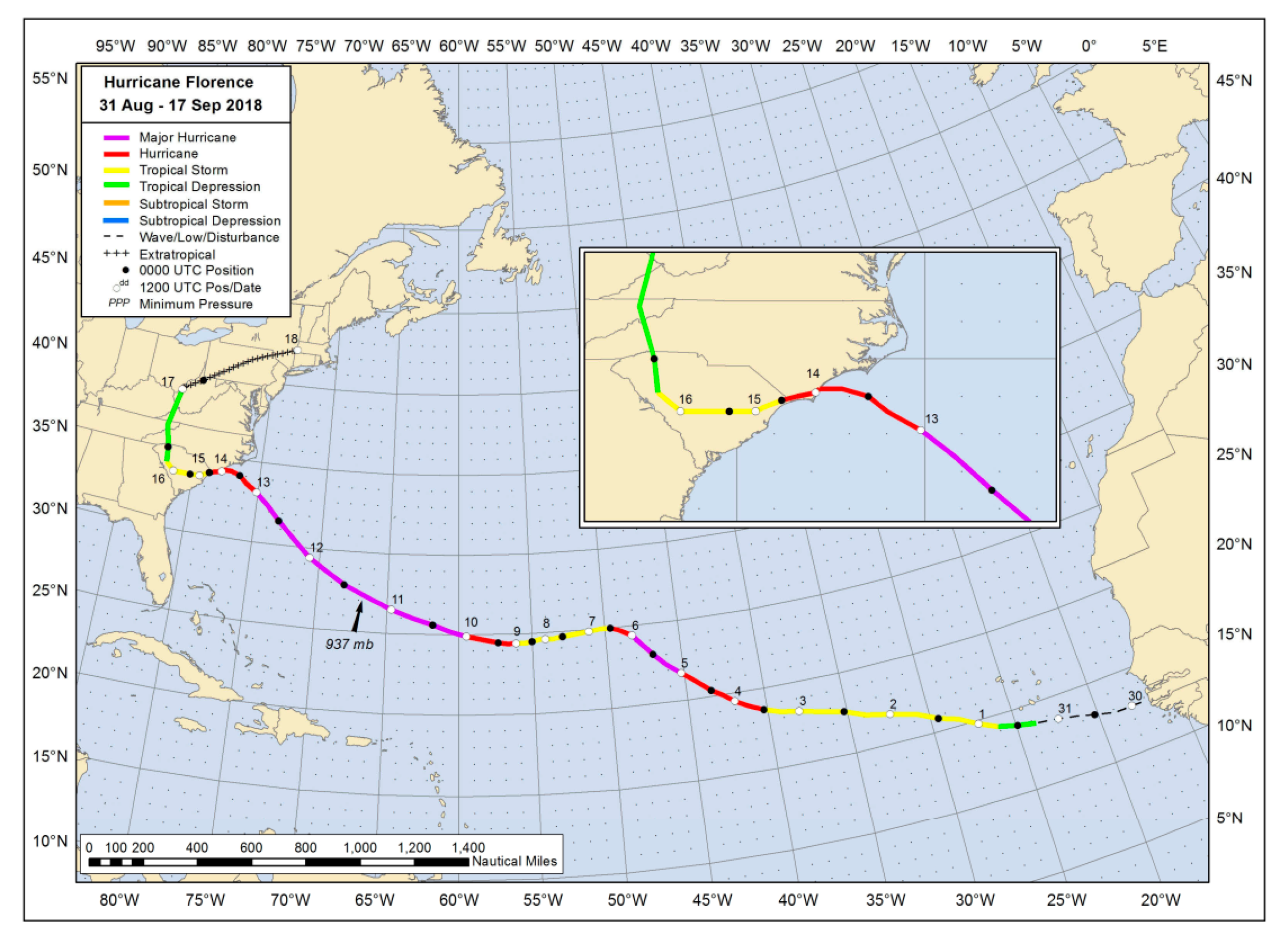
In this section, we take Hurricane Florence as an example to demonstrate how to process the aforementioned observation data to fix the center of a TC and to estimate its intensity. Hurricane Florence originated from a large tropical wave that departed off the west coast of Africa on 30 August, 2018 and reached tropical storm status on 1 September 2018. Its wind speed increased to 33.3 m/s on September 9 and weakened to 30.8 m/s on September 15 [33]. To examine the evolving stage of Hurricane Florence, the SMAP radiometer data and the CYGNSS data that were acquired from 8 to 12 September 2018 were employed for TC observations. The best track of Hurricane Florence was provided by the National Hurricane Center (NHC) [33] and this was used for validation, as shown in Figure 3, and its observation region was chosen as 44° to 80° W longitude and 20° to 32° N latitude.
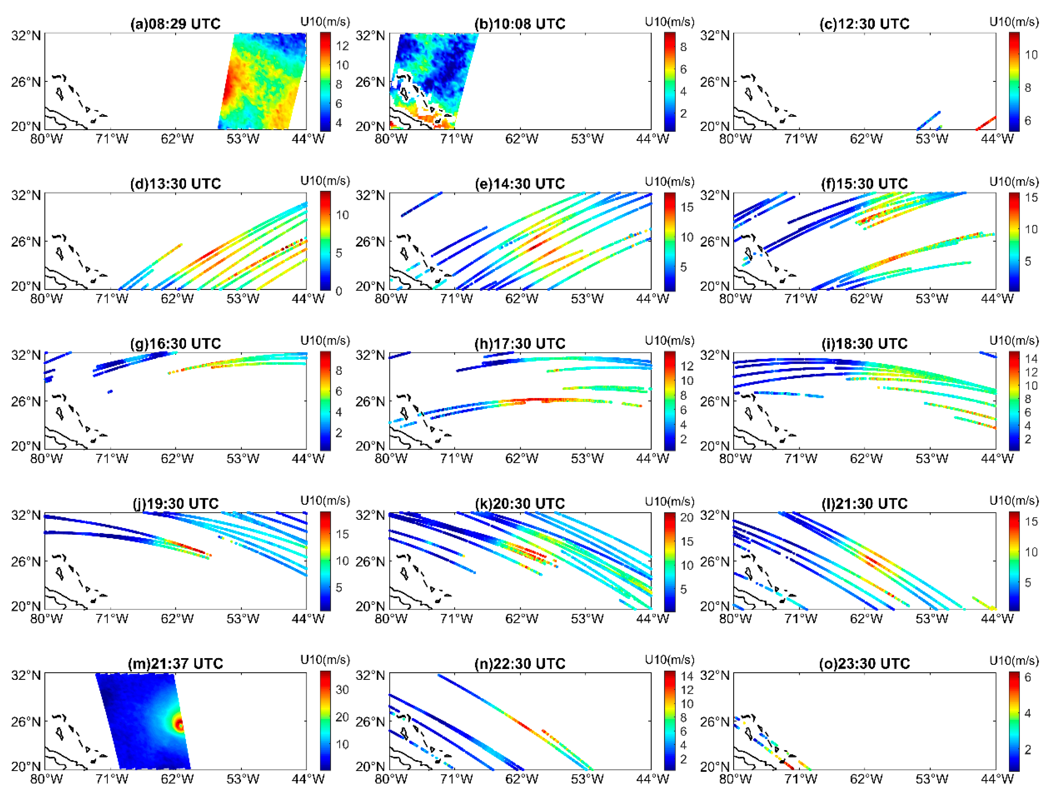
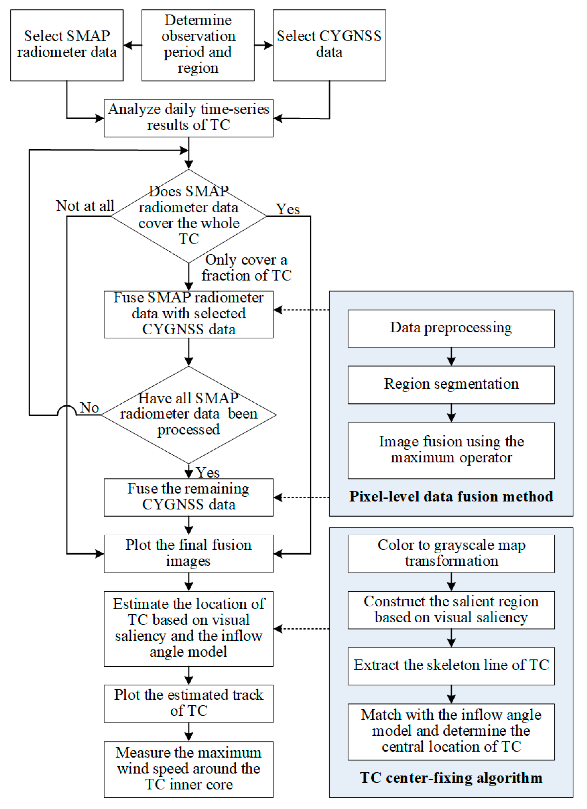
The time-series results for Hurricane Florence, which were obtained over the selected observation region on 10 September 2018 using the SMAP satellite and CYGNSS constellation, are shown in Figure 4. The SMAP radiometer can only acquire two samples over the selected observation area, which correspond to its ascending and descending passes, and the time interval between these two samples is about 12 h. On the other hand, although the SMAP radiometer has a wide swath, it cannot always acquire the complete structure of a TC. For example, as shown in Figure 4b, Hurricane Florence was not captured by the SMAP radiometer. Another example is shown in Figure 4m, where only a fraction of Hurricane Florence was captured by the SMAP radiometer. Since the CYGNSS constellation consists of eight low earth-orbiting microsatellites, the median value of the revisit time is 2.8 h and the mean revisit time is 7.2 h. Furthermore, it can produce 32 specular reflections per second, leading to 32 separate tracks which are 25 km wide and typically hundreds of kilometers long [29]. Thus, compared to the SMAP radiometer, the CYGNSS constellation is able to take more samples (thirteen samples in Figure 4) of a TC over the same region to significantly shorten the observation interval and it can also measure the ocean surface wind speed over a larger observation area. Nevertheless, as can be seen from Figure 4, it is difficult to accurately fix the center of the TC with any CYGNSS sample because of the sparse tracks of CYGNSS satellite. Therefore, a data fusion method was used to obtain a complete structure of the TC. A flowchart of the data processing is shown in Figure 5, and each step is described below.
The first step of data processing is to analyze the daily time-series results for TCs obtained during the observation period. In this step, the following three cases were considered:
- ●
- Case 1. If a result is obtained by the SMAP radiometer and it contains a complete structure of a TC or none at all, it is reserved with no further processing, similar to the two examples shown in Figure 6. This is because the observation results obtained by the SMAP radiometer provide a better visualization to analyze the TC position than those acquired by the CYGNSS constellation.
- ●
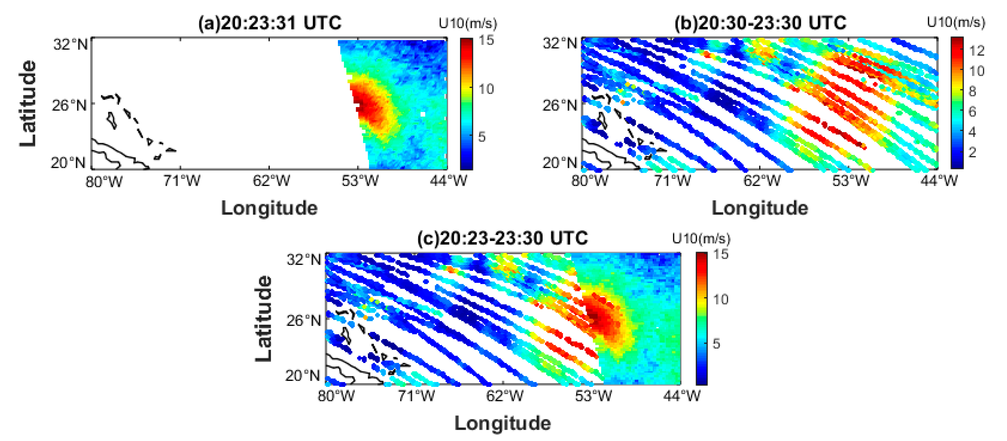
- Case 2. If a result is obtained by the SMAP radiometer and contains only a fraction of the TC, it will be fused with several CYGNSS observation results to obtain the complete structure of the TC. Here, the CYGNSS data used for data fusion were acquired around the time when the aforementioned SMAP radiometer results were obtained. Note that the time interval during which the CYGNSS data were intercepted for data fusion is determined by the movement speed of hurricane. In other words, a faster hurricane speed corresponds to a shorter time interval used for the CYGNSS data interception. For example, only a fraction of Hurricane Florence was captured by the SMAP radiometer at 20:23 UTC on 11 September 2018. Since the central location of the hurricane can be roughly estimated according to the high wind speed region shown in most SMAP radiometer and CYGNSS data, such as Figure 4l–m, the difference in the spatial location of the hurricane between the adjacent SMAP radiometer and CYGNSS data can be obtained. At the same time, the time interval between these two data can also be easily calculated. As a result, the speed of the hurricane can be obtained in terms of the difference in its spatial location and the corresponding time interval. After a rough estimate of Hurricane Florence’s speed, the CYGNSS data acquired from 20:30 to 23:30 UTC were chosen for data fusion, as shown in Figure 7.
- ●
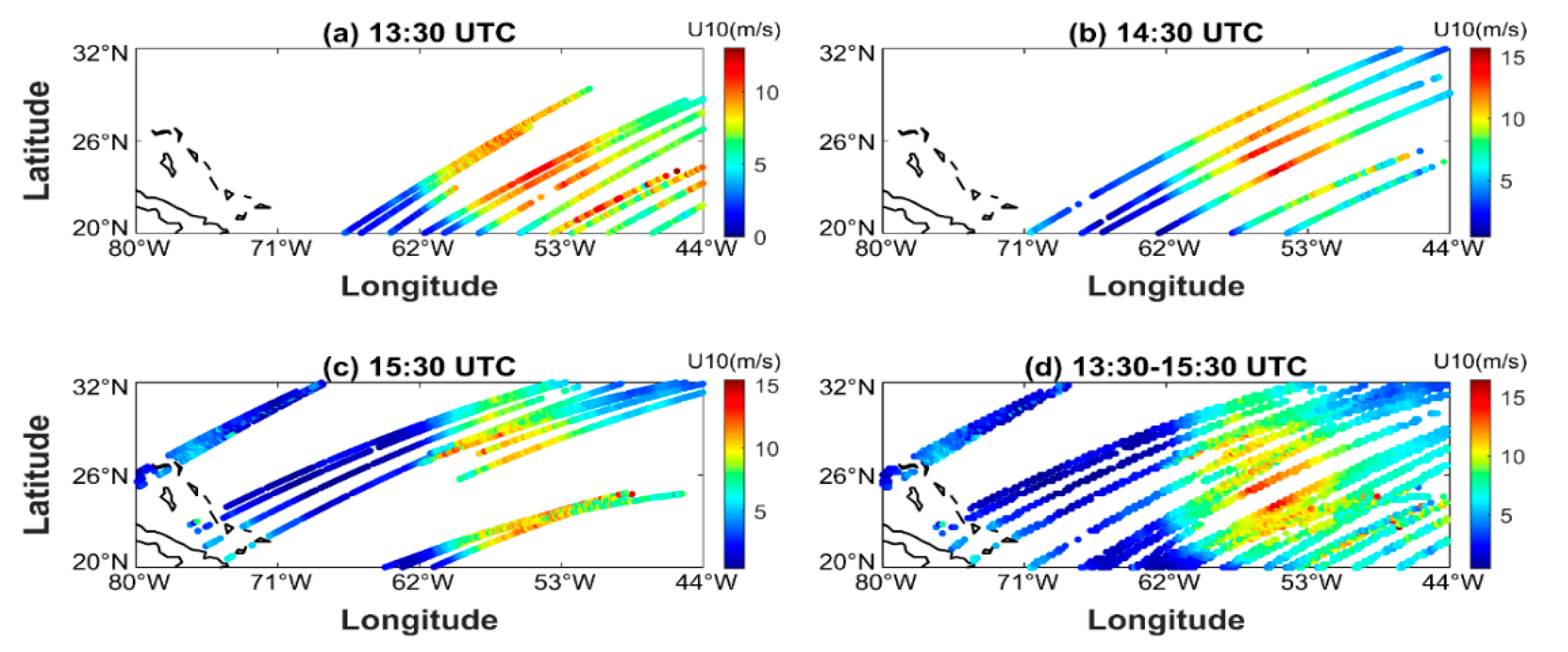
- Case 3. In addition to the observation data already used in the above cases, the remaining CYGNSS data are also fused in terms of the movement speed of the hurricane to provide a better visualization of the TC for fixing its center due to the sparse tracks of CYGNSS satellite. An example is shown in Figure 8. After a rough estimate of Hurricane Florence’s speed on 9 September 2018, we selected the CYGNSS data acquired from 13:30 to 15:30 UTC for data fusion. The method used here to roughly estimate the speed of hurricane is the same as that described in Case 2.
The second step is data fusion, i.e., fusing the SMAP radiometer and CYGNSS data or only the CYGNSS data, as mentioned in the first step. A pixel-level data fusion method, which is similar to the region-based fusion method described in [34], was used in this study. The essential problem of pixel-level fusion can be defined as
where , ,…, represents N images capturing the same region, is the fusion operator, which are typically represented by mean and maximum operators.
Data preprocessing is the first step in data fusion. Here, both SMAP radiometer data and CYGNSS data were averaged in space on a 0.2° latitude and longitude grid, and then the image registration was performed due to the differences in the acquisition time and configuration of each result. In addition, a unified scale was adopted for the surface wind speeds retrieved from the SMAP radiometer and CYGNSS data. After data preprocessing, a single result was divided into two parts using a threshold segmentation, i.e., the region-of-interest (ROI) and non-ROI. Here, ROI was defined as a region with a high pixel value because it may be a TC. The rest of the pixels were defined as a non-ROI because they cannot provide any useful information related to a TC. The minimum wind speed of a TC was set as the threshold used for region segmentation. Following the region segmentation, both the ROI and non-ROI in all images used for data fusion were fused by the maximum operator, and this process can be written as
where represents the final fusion image, denotes the maximum operator, and denotes the position of a pixel.
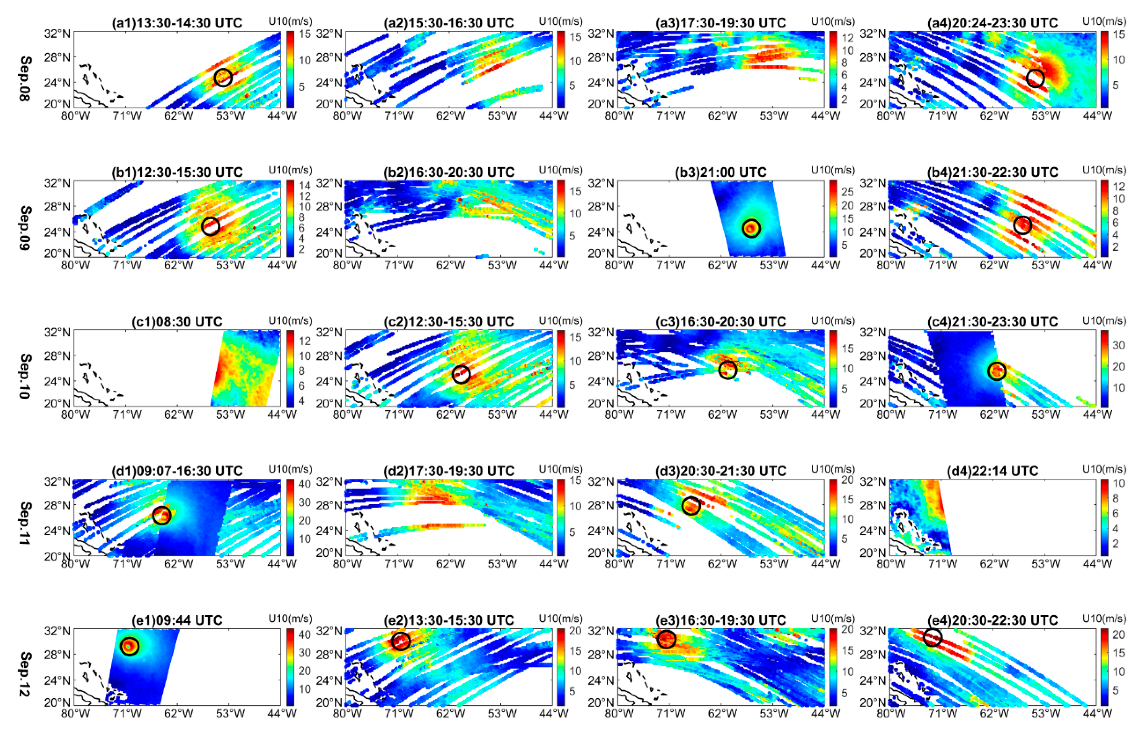
Thus, the final fusion image can be obtained, such as the composite images displayed in Figure 7 and Figure 8. It can be clearly seen from Figure 8 that it is difficult to fix the center of Hurricane Florence using the three results acquired at 13:30 UTC, 14:30 UTC, and 15:30 UTC, respectively. However, the complete structure of Hurricane Florence can be obtained through data fusion. After processing all the observation data, the daily observation results were plotted in turn in each row of the final image, as shown in Figure 9.
The third step involves estimating the TC location. When Hurricane Florence is completely included in the SMAP radiometer data, as shown in Figure 9b, its diameter can be directly measured in terms of its shape. We found that its diameter was about 145 km, and hence a black circle with a radius of 150 km was adopted to fix its center position, similar to the marking method described in [35]. Since the surface winds are always strongest along the margin of the TC eye [36], the location of this black circle was automatically determined in terms of the shape of the high wind-speed region and the movement speed of TC. Here, the automatic TC center-fixing algorithm, which was applied to the SMAP and CYGNSS fusion results, is based on visual saliency and the inflow angle model, similar to the method used for center location of typhoons in SAR images [37]. In this algorithm, each color image shown in Figure 9 was first transformed into a grayscale map to make it similar to SAR images by using the weighted average. Then, with regard to the gray-level feature, the salient region corresponding to the high wind-speed region was constructed in the grayscale map based on the visual saliency. Then, the skeleton line of the TC was extracted according to the shape of the salient region and the movement speed of the TC. Finally, the skeleton line of the TC was matched with the inflow angle model to determine the central position of the TC [37]. Nevertheless, it is still difficult to fix the center of the TC with some fusion results, such as shown in Figure 9(a2), not only due to the sparse and narrow tracks of CYGNSS satellite but also because sometimes the incomplete structure of a TC was included in such fusion results. Finally, the point, which is the center of the black circle, was further extracted to form the estimated track of TC.
The final step includes measuring the maximum wind speed around the TC inner core. If a complete structure of the TC was included in the SMAP radiometer data, the maximum wind speed in the region marked by the black circle was obtained directly from the SMAP radiometer data. If the CYGNSS and SMAP radiometer data were combined to obtain a complete structure of the TC, the black circle contains a fraction of the CYGNSS data and a part of the SMAP radiometer data (see Figure 9(d1)), therefore, the CYGNSS Level 2 data products derived by the YSLF GMF and the SMAP radiometer data were used to search for the corresponding maximum wind speed at the pixel level. Then, these two results were compared with each other to obtain the final maximum wind speed in the region marked by the black circle. If only the CYGNSS data were fused to observe TCs, the maximum wind speed in the region marked by the black circle was obtained directly from the Level 2 data products derived by the YSLF GMF.
4. Results
4.1. TC Track Estimation
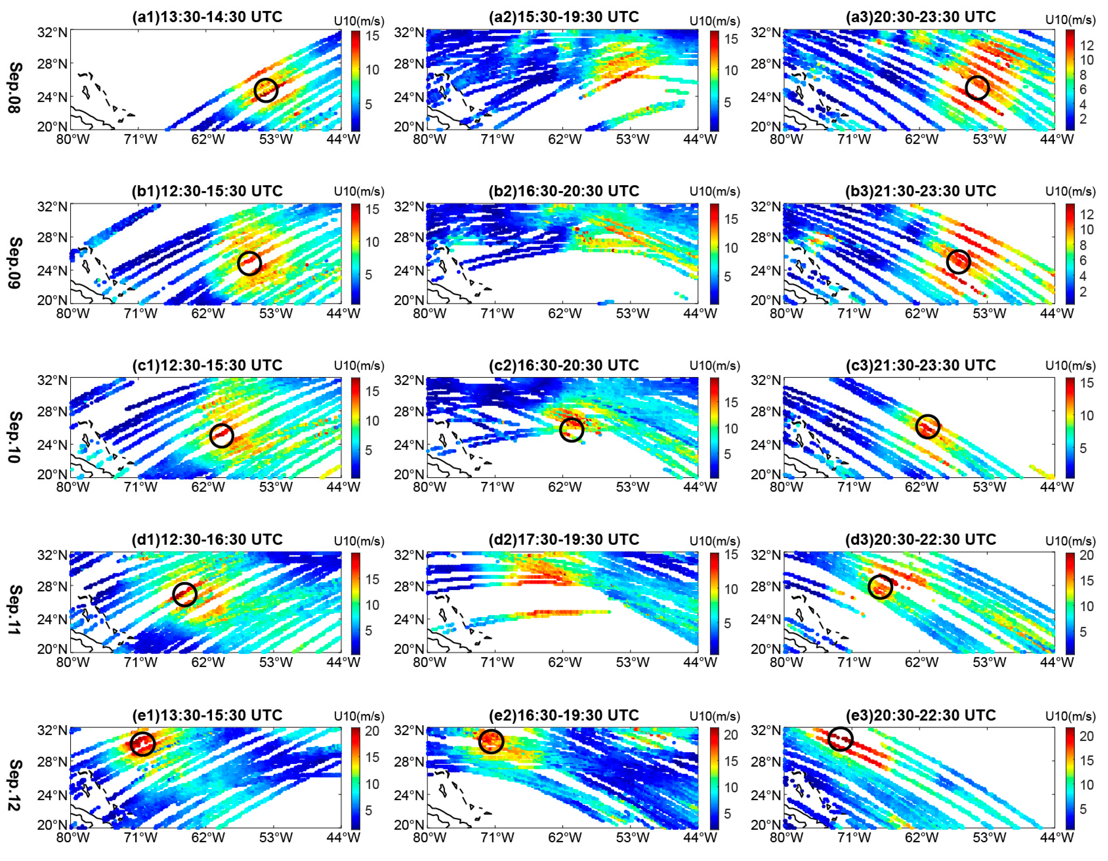
When the SMAP radiometer and CYGNSS data were combined to estimate the position of Hurricane Florence, the final fusion image was obtained and this is shown in Figure 9. To maintain data integrity, the observation results were obtained individually by the SMAP satellite or CYGNSS constellation and did not contain any information about the TC; these are also presented below. As shown in Figure 9, the joint use of the SMAP radiometer and CYGNSS data provides better visualization of TCs, and TCs can be observed with a higher temporal resolution compared to the case where only the SMAP radiometer was used to monitor TCs. The final fusion image, which was obtained by only fusing the CYGNSS data according to the movement speed of the hurricane, is presented in Figure 10. A comparison with Figure 9 shows that the number of fusion results decreased and the visualization of TC also became worse due to the narrow tracks of the CYGNSS satellite. Note that the location of the black circle was automatically determined (see Figure 10) in relation to the shape of high wind-speed region and the movement speed of the TC by using the TC center-fixing algorithm described in Section 3.
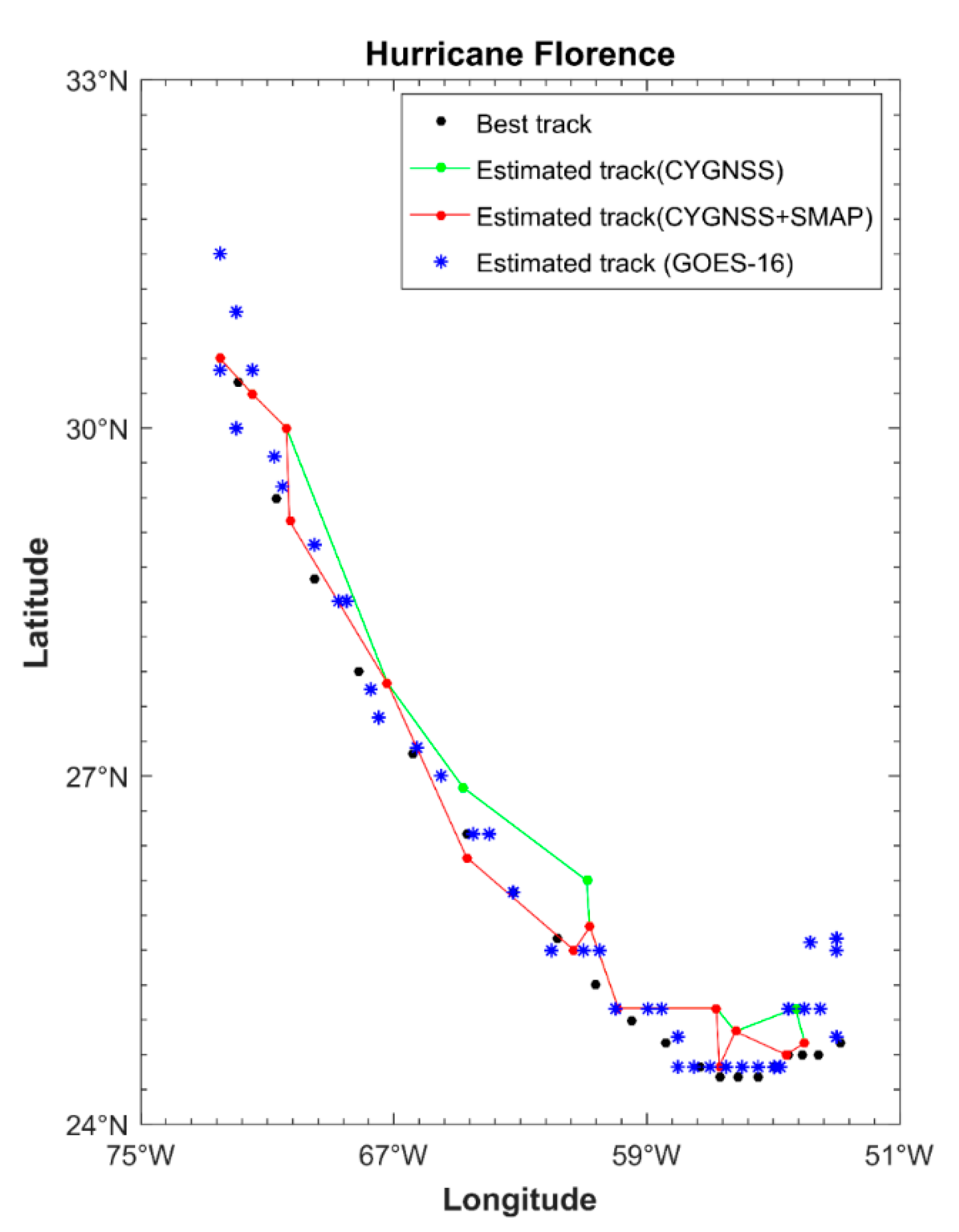
According to the processing method described in Section 3, we estimated the track of Hurricane Florence from Figure 9 and Figure 10. Additionally, a comparison between the estimated and NHC best tracks of Hurricane Florence is illustrated in Figure 11. Figure 11 clearly shows that the TC track obtained by fusing the SMAP radiometer data and the CYGNSS data is more consistent with the NHC best track than that obtained by only fusing the CYGNSS data. A more detailed comparison between the estimated and NHC best tracks of Hurricane Florence is given in Table 1. Furthermore, another nine hurricanes were analyzed in the same way as Hurricane Florence, and the results of this analysis are also listed in Table 1. Here, the mean absolute error (MAE) and the standard deviation (SD) were estimated by calculating the distance between the estimated center of hurricane and that obtained from the NHC best track data. Note that the NHC best tracks for all hurricanes observed can be accessed at https://www.nhc.noaa.gov/data/tcr/.
Table 1 shows the comparison between the TC tracks obtained by fusing the SMAP radiometer and CYGNSS data and the NHC best tracks. The MAE values range between 18.4 and 46 km, the SD values vary between 15.1 and 28.2 km, and both of them are smaller than those obtained by only fusing the CYGNSS data.
4.2. Maximum Wind Speed Measurement
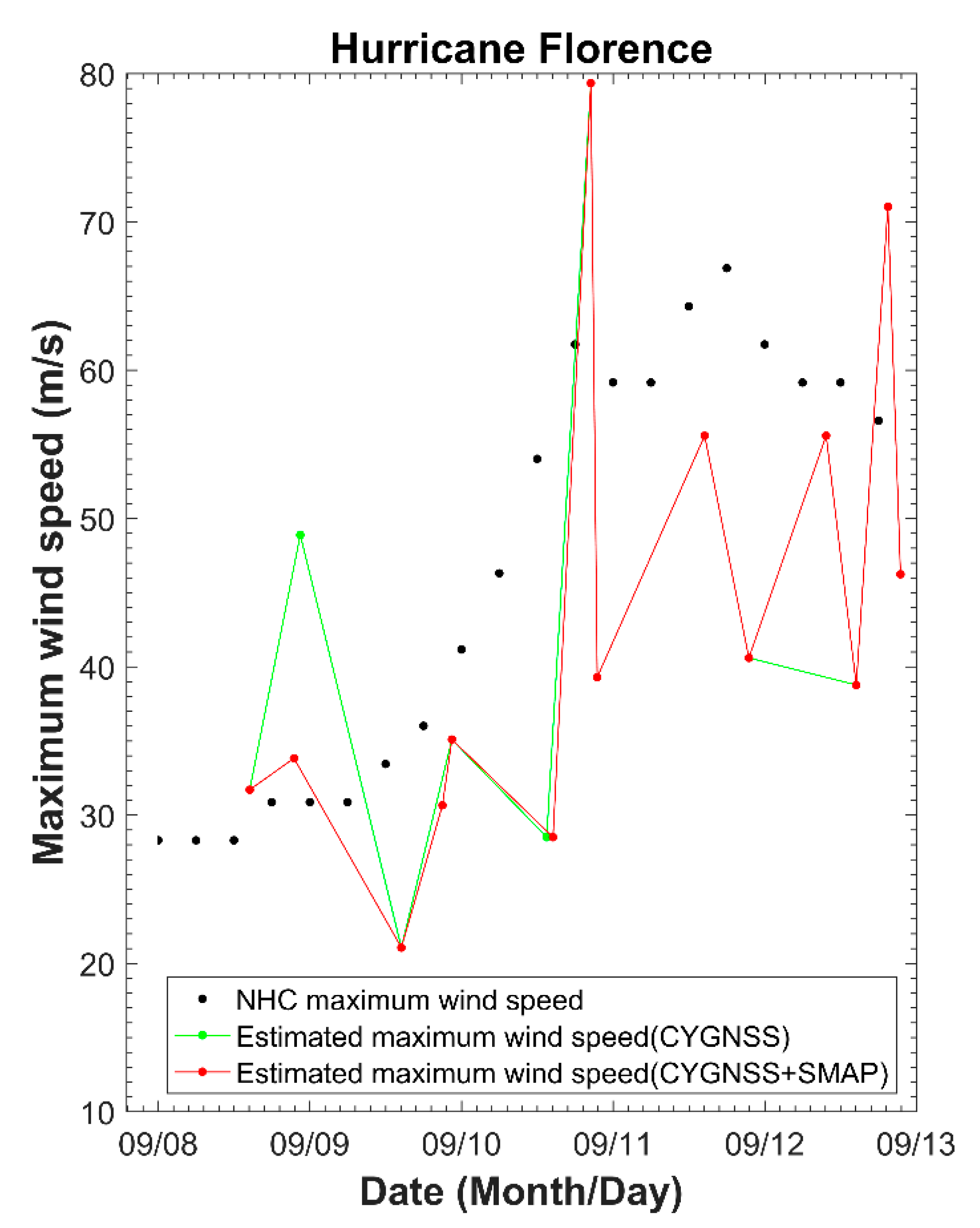
According to the processing method described in Section 3, we estimated the maximum wind speeds of Hurricane Florence from Figure 9 and Figure 10. A comparison between the estimated maximum wind speeds of Hurricane Florence and the best track peak winds estimated by the NHC [33] is shown in Figure 12. Here, a time interpolation method was applied to the estimated maximum wind speeds to ensure that the estimated and NHC wind speeds used for the comparison were obtained at the same time.
It can be clearly seen from Figure 12 that the maximum wind speeds of Hurricane Florence can be measured at more frequent intervals by fusing the SMAP radiometer and CYGNSS data than in the case of only fusing the CYGNSS data. Furthermore, the measured maximum wind speeds are in better agreement with the NHC best track peak wind speeds than those obtained by only fusing the CYGNSS data. A more detailed comparison between the estimated and NHC maximum wind speeds of Hurricane Florence is given in Table 2. The other nine hurricanes were analyzed in the same way as Hurricane Florence, and the results of this analysis are also listed in Table 2. Here, the root-mean-square difference (RMSD), the MAE, the correlation coefficient, and the bias were adopted to analyze the difference between the estimated and NHC maximum wind speeds of each hurricane. Note that the NHC best track peak wind speeds of all observed hurricanes can be accessed at https://www.nhc.noaa.gov/data/tcr/.
As shown in Table 2, when we compared the maximum wind speeds obtained by fusing the SMAP radiometer and CYGNSS data with the best track peak winds estimated by the NHC, we found that the MAE values ranged between 7.7 and 15.7 m/s, the RMSD values varied between 8.6 and 18 m/s, the correlation coefficients ranged between 0.1782 and 0.9877, the bias values varied between −8.5 and 4.5 m/s, and all of these were smaller than those obtained by only fusing the CYGNSS data, except for Hurricanes Dorian and Michael. This is due to the fact that Hurricanes Dorian and Michael made multiple landfalls during the observation period, and the SMAP radiometer can only measure the ocean surface wind speed, which results in a large difference between the estimated and NHC maximum wind speeds.
5. Discussion
When the SMAP radiometer and CYGNSS data were combined to estimate the position of Hurricane Florence, the black circle does not appear in some subfigures of Figure 9, for example, Figure 9(a2). This is due to the fact that the fusion result shown in such subfigures does not contain a complete structure of the TC, mainly because of the sparse tracks of CYGNSS satellites. As a result, the TC center-fixing algorithm cannot determine the center position of the TC. Furthermore, when our method was used to estimate the tracks of the ten hurricanes listed in Table 1 compared to the NHC best tracks, the MAE values range between 18.4 and 46 km, and the SD values vary between 15.1 and 28.2 km. To further evaluate the performance of our method, a comparison of the track of Hurricane Florence estimated with GOES-16 GeoColor images using the Automated Rotational Center Hurricane EYE Retrieval (ARCHER) TC center-fixing algorithm [38] was also made, as shown in Figure 11. We found that the MAE was 40.1 km and the SD was 25.1 km. In addition, compared to the TC center automatic determination method based on HY-2 and QuikSCAT wind vector products that is described in [39], our method achieves higher accuracy in the estimation of the TC track according to the MAE and SD values, and it can also monitor the TC track with a shorter time interval because of the combination of the CYGNSS data. It is worth mentioning here that the wind direction parameter included in the SMAP radiometer data is not added to estimate the center position of TCs at this stage because this parameter has not been provided in the CYGNSS data yet.
The errors produced by fusing the SMAP radiometer and CYGNSS data to track TCs are mainly due to the following reasons.
(1) Although a complete structure of the TC has been included in the final fusion image, it is still difficult to determine the center location of the TC because of the large high-speed region presented in CYGNSS fusion results, such as in Figure 9(b1).
(2) Since the size of a TC eye can vary from a few to tens of kilometers, even up to hundreds of kilometers [40], it is difficult to accurately fix the center of the TC with a point that is the center of black circle and which was used to form the estimated track of the TC in this study.
(3) In terms of the shape of the high wind-speed region and the movement speed of the TC, the automatic TC center-fixing algorithm based on visual saliency and the inflow angle model were applied to the SMAP and CYGNSS fusion results. However, we found that this algorithm introduced errors in the estimation of TC’s center position because sometimes the extracted skeleton line of the TC cannot be well-matched with the inflow angle model.
Besides the aforementioned factors, changes in the spatial-temporal resolution of the observation data can also affect the accuracy of the TC track estimation results, as reported by Omranian et al. [41]. On one hand, observation data with a high temporal resolution are very important for the estimation of the TC track during the rapidly evolving stages of a TC’s life cycle. As shown in Figure 4, the joint use of SMAP radiometer and CYGNSS data significantly improves the temporal resolution compared to the case in which only the SMAP radiometer data are used. However, when the SMAP radiometer and CYGNSS data were fused to obtain a complete structure of the TC to determine its center position, the temporal resolution was reduced to a large extent. On the other hand, observation data with a high spatial resolution are also very helpful for the estimation of the TC’s center position because the fine structure of TCs can be obtained. However, since the grid size of the SMAP radiometer and CYGNSS data used in our study is fixed, more attention was paid to the spatial coverage to obtain a more complete structure of the TCs. As can be seen from Figure 9, the observation data with larger spatial coverage can improve the accuracy of fixing the center position of TCs.
When our method was used to measure the maximum wind speeds of the ten hurricanes listed in Table 2, intensity errors were produced mainly due to the following reasons.
(1) Sometimes a complete structure of the TC was not included in the CYGNSS fusion results due to the narrow and sparse tracks of the CYGNSS satellite, as well as its limited spatial coverage [42]. As a result, the maximum wind speed area was not always sampled by the CYGNSS constellation, for example, Hurricane Lane.
(2) Some of the observed hurricanes, such as Hurricane Harvey, made landfall during the observation period. In other words, the maximum wind speed areas were on land; however, both SMAP radiometer and CYGNSS satellites can only measure the ocean surface wind speed, as mentioned above.
(3) Compared with the moored buoy data, the ocean surface wind speed retrieval algorithms adopted for the SMAP radiometer data [31] and also the CYGNSS data [43] can introduce errors, especially for wind speeds above 20 m/s.
Besides the above factors, the selection of appropriate spaceborne microwave sensor data can also affect the accuracy of the maximum wind speed measurements. Although various spaceborne microwave sensors have been developed to observe the TCs, however, many of them cannot measure Category 1 hurricanes and more powerful storms except for the SMAP radiometer, the Soil Moisture and Ocean Salinity (SMOS) radiometer [44], the CYGNSS satellite, and some spaceborne SARs [45]. For example, when the Metop Advanced SCATterometer (ASCAT) data are used to measure the wind speed above 20 m/s, a reliable estimation of TC intensity cannot be provided [46]. However, these spaceborne microwave sensors can be employed to measure the TC intensity during its early stages. In addition, as pointed out by Omranian et al. [47], heavy rain can also affect the sounding performance of spaceborne microwave sensors except for these operating at a lower frequency.
6. Conclusions
This paper presented the joint use of a spaceborne microwave sensor and the CYGNSS constellation to observe TCs. The observation results demonstrated that compared to the case where only the spaceborne microwave sensor data or the CYGNSS data were used to observe TCs, the proposed method obtains a more complete structure of the TC and can measure the surface wind speed around the TC inner core at more frequent intervals. Furthermore, the TC tracks obtained by the proposed method are in better agreement with the NHC best tracks, and the maximum wind speeds around the TC inner core obtained by the proposed method are more consistent in most cases with the best track peak winds estimated by the NHC. In future work, more observation data from the microwave sensors, such as the SMOS radiometer and the spaceborne SAR, and the wind direction parameter will be combined to further improve the spatial coverage, the temporal resolution, and the measurement accuracy of the maximum wind speed around the TC inner core. Furthermore, for the observation results obtained by fusing the data from the CYGNSS and meteorological satellites, a spatial interpolation method and an automatic TC center-fixing algorithm based on deep learning will be developed to solve the problems related to the sparse tracks of the GYGNSS satellite and to improve the accuracy of tracking TCs.
Author Contributions
Conceptualization, S.S.; methodology, S.S. and S.W.; data collection and data analysis, S.W.; writing—original draft preparation, S.W. and S.S.; writing—review and editing, B.N. All authors have read and agree to the published version of the manuscript.
Funding
This research was supported by the National Natural Science Foundation of China (41504007).
Acknowledgments
The authors would like to thank the anonymous reviewers for their helpful comments and suggestions.
Conflicts of Interest
The authors declare no conflict of interest.
References
- Khalil, G.M. Cyclones and storm surges in Bangladesh: Some mitigative measures. Nat. Hazards 1992, 6, 11–24. [Google Scholar] [CrossRef]
- Zhang, P. The Chinese meteorological satellite and applications. In Proceedings of the International Geoscience and Remote Sensing Symposium (IGARSS), Beijing, China, 10–15 July 2016; pp. 5516–5517. [Google Scholar]
- Gaiser, P.W.; St. Germain, K.M.; Twarog, E.M.; Poe, G.A.; Purdy, W.; Richardson, D.; Grossman, W.; Jones, W.L.; Spencer, D.; Golba, G.; et al. The WindSat spaceborne polarimetric microwave radiometer: Sensor description and early orbit performance. IEEE Trans. Geosci. Remote Sens. 2004, 42, 2347–2361. [Google Scholar] [CrossRef]
- Wang, X.; Liu, L.; Shi, H.; Dong, X.; Zhu, D. In-orbit calibration and performance evaluation of HY-2 scatterometer. In Proceedings of the International Geoscience and Remote Sensing Symposium (IGARSS), Munich, Germany, 22–27 July 2012; pp. 4614–4616. [Google Scholar]
- Shen, H.; Perrie, W.; He, Y. Evaluation of hurricane wind speed retrieval from cross-dual-pol SAR. Int. J. Remote Sens. 2016, 37, 599–614. [Google Scholar] [CrossRef]
- Hu, T.; Zhang, D.; Wang, J.; Zhang, Y. Review of Typhoon monitoring technology based on remote sensing satellite data. Remote Sens. Technol. Appl. 2013, 28, 994–999. [Google Scholar]
- Martin-Neira, M. A passive reflectometry and interferometry system (PARIS): Application to ocean altimetry. ESA J. 1993, 17, 331–335. [Google Scholar]
- Zavorotny, V.U.; Voronovich, A.G. Scattering of GPS signals from the ocean with wind remote sensing application. IEEE Trans. Geosci. Remote Sens. 2000, 38, 951–964. [Google Scholar] [CrossRef] [Green Version]
- Marchan-Hernandez, J.F.; Camps, A.; Rodriguez-Alvarez, N.; Valencia, E.; Bosch-Lluis, X.; Ramos-Perez, I. An efficient algorithm to the simulator of Delay-Doppler maps of reflected global navigation satellite system signals. IEEE Trans. Geosci. Remote Sens. 2009, 47, 2733–2740. [Google Scholar] [CrossRef]
- Martin-Neira, M.; D’Addio, S.; Buck, C.; Floury, N.; Prieto-Cerdeira, R. The PARIS ocean altimeter in-orbit demonstrator. IEEE Trans. Geosci. Remote Sens. 2011, 49, 2209–2237. [Google Scholar] [CrossRef]
- Jin, S.; Feng, G.P.; Gleason, S. Remote sensing using GNSS signals: Current status and future directions. Adv. Space Res. 2011, 47, 1645–1653. [Google Scholar] [CrossRef]
- Gleason, S.; Hodgart, S.; Sun, Y.; Gommenginger, C.; Mackin, S.; Adjrad, M.; Unwin, M. Detection and processing of bistatically reflected GPS signals from low earth orbit for the purpose of ocean remote sensing. IEEE Trans. Geosci. Remote Sens. 2005, 43, 1229–1241. [Google Scholar] [CrossRef] [Green Version]
- Ruf, C.; Lyons, A.; Unwin, M.; Dickinson, J.; Rose, R.; Rose, D.; Vincent, M. CYGNSS: Enabling the future of hurricane prediction. IEEE Geosci. Remote Sens. Mag. 2013, 1, 52–67. [Google Scholar] [CrossRef]
- Ruf, C.; Gleason, S.; Ridley, A.; Rose, R.; Scherrer, J. The NASA CYGNSS mission: Overview and status update. In Proceedings of the International Geoscience and Remote Sensing Symposium (IGARSS), Fort Worth, TX, USA, 23–28 July 2017; pp. 2641–2643. [Google Scholar]
- Gleason, S.; Ruf, C.S.; O’Brien, A.J.; McKague, D.S. The CYGNSS level 1 calibration algorithm and error analysis based on on-orbit measurements. IEEE J. Sel. Top. Appl. Earth Observ. Remote Sens. 2019, 12, 37–49. [Google Scholar] [CrossRef]
- Clarizia, M.P.; Ruf, C.S. Wind speed retrieval algorithm for the cyclone global navigation satellite system (CYGNSS) mission. IEEE Trans. Geosci. Remote Sens. 2016, 54, 4419–4432. [Google Scholar] [CrossRef]
- Ruf, C.S.; Gleason, S.; McKague, D.S. Assessment of CYGNSS wind speed retrieval uncertainty. IEEE J. Sel. Top. Appl. Earth Observ. Remote Sens. 2019, 12, 87–97. [Google Scholar] [CrossRef]
- Morris, M.; Ruf, C.S. Determining tropical cyclone surface wind speed structure and intensity with the CYGNSS satellite constellation. J. Appl. Meteorol. Climatol. 2017, 56, 1847–1865. [Google Scholar] [CrossRef]
- Mayers, D.; Ruf, C. Tropical cyclone center fix using CYGNSS winds. J. Appl. Meteorol. Climatol. 2019, 58, 1993–2003. [Google Scholar] [CrossRef]
- Morris, M.; Ruf, C.S. Estimating tropical cyclone integrated kinetic energy with the CYGNSS satellite constellation. J. Appl. Meteorol. Climatol. 2017, 56, 235–245. [Google Scholar] [CrossRef]
- Said, F.; Soisuvarn, S.; Jelenak, Z.; Chang, P.S. Performance assessment of simulated CYGNSS measurements in the tropical cyclone environment. IEEE J. Sel. Top. Appl. Earth Observ. Remote Sens. 2016, 9, 4709–4719. [Google Scholar] [CrossRef]
- Said, F.; Katzberg, S.J.; Soisuvarn, S. Retrieving hurricane maximum winds using simulated CYGNSS power-versus-delay waveforms. IEEE J. Sel. Top. Appl. Earth Observ. Remote Sens. 2017, 10, 3799–3809. [Google Scholar] [CrossRef]
- Crespo, J.A.; Posselt, D.J.; Naud, C.M.; Bussy-Virat, C. Assessing CYGNSS’s potential to observe extratropical fronts and cyclones. J. Appl. Meteorol. Climatol. 2017, 56, 2027–2034. [Google Scholar] [CrossRef]
- Zhang, S.; Pu, Z.; Posselt, D.J.; Atlas, R. Impact of CYGNSS ocean surface wind speeds on numerical simulations of a hurricane in observing system simulation experiments. J. Atmos. Ocean. Technol. 2017, 34, 375–383. [Google Scholar] [CrossRef]
- Ruf, C.S.; Chew, C.; Lang, T.; Morris, M.G.; Nave, K.; Ridley, A.; Balasubramaniam, R. A new paradigm in earth environmental monitoring with the CYGNSS small satellite. Sci. Rep. 2018, 8, 8782. [Google Scholar] [CrossRef] [PubMed] [Green Version]
- Cui, Z.; Pu, Z.; Tallapragada, V.; Atals, R.; Ruf, C.S. A preliminary impact study of CYGNSS ocean surface wind speeds on numerical simulations of hurricanes. Geophys. Res. Lett. 2019, 46, 2984–2992. [Google Scholar] [CrossRef] [PubMed] [Green Version]
- Ruf, C.; Asharaf, S.; Balasubramaniam, R.; Gleason, S.; Lang, T.; McKague, D.; Twigg, D.; Waliser, D. In-orbit performance of the constellation of CYGNSS hurricane satellites. Bull. Amer. Meteorol. Soc. 2019, 100, 2009–2023. [Google Scholar] [CrossRef]
- Li, X.; Mecikalski, J.R.; Lang, T.J. A study on assimilation of CYGNSS wind speed data for tropical convection during 2018 January MJO. Remote Sens. 2020, 12, 1243. [Google Scholar] [CrossRef] [Green Version]
- Ruf, C.; Chang, P.S.; Clarizia, M.P.; Gleason, S.; Jelenak, Z.; Majumdar, S.; Morris, M.; Murray, J.; Musko, S.; Posselt, D.; et al. CYGNSS Handbook, 1st ed.; Michigan Publishing: Ann Arbor, MI, USA, 2016; pp. 20–108. [Google Scholar]
- Ruf, C.S.; Balasubramaniam, R. Development of the CYGNSS geophysical model function for wind speed. IEEE J. Sel. Topics Appl. Earth Observ. Remote Sens. 2019, 12, 66–77. [Google Scholar] [CrossRef]
- Meissner, T.; Ricciardulli, L.; Wentz, F.J. Capability of the SMAP mission to measure ocean surface winds in storms. Bull. Amer. Meteor. Soc. 2017, 98, 1660–1677. [Google Scholar] [CrossRef]
- Yueh, S.H.; Fore, A.G.; Tang, W.; Hayashi, A.; Stiles, B.; Reul, N.; Weng, Y.; Zhang, F. SMAP L-band passive microwave observations of ocean surface wind during severe storms. IEEE Trans. Geosci. Remote Sens. 2016, 54, 7339–7350. [Google Scholar] [CrossRef]
- National Hurricane Center Tropical Cyclone Report: Hurricane Florence. Available online: http://www.nhc.noaa.gov/data/tcr/AL062018_Florence.pdf (accessed on 22 March 2020).
- Zeng, T.; Ao, D.; Hu, C.; Zhang, T.; Liu, F.; Tian, W.; Lin, K. Multiangle BSAR imaging based on BeiDou-2 navigation satellite system: Experiments and preliminary results. IEEE Trans. Geosci. Remote Sens. 2015, 53, 5760–5773. [Google Scholar] [CrossRef]
- Lu, X.; Yu, H.; Yang, X.; Li, X. Estimating tropical cyclone size in the Northwestern Pacific from geostationary satellite infrared images. Remote Sens. 2017, 9, 728. [Google Scholar] [CrossRef] [Green Version]
- Newnham, E.V. The tropical cyclone. Nature 1926, 118, 524–526. [Google Scholar] [CrossRef]
- Jin, S. Center Location of Typhoons in SAR Images Based on Visual Saliency and Feature Learning. Ph.D. Thesis, XiDian University, Xi’an, China, September 2016. [Google Scholar]
- Wimmers, A.J.; Velden, C.S. Advancements in objective multisatellite tropical cyclone center fixing. J. Appl. Meteorol. Climatol. 2016, 55, 197–212. [Google Scholar]
- Hu, T.; Wu, Y.; Zheng, G.; Zhang, D.; Zhang, Y.; Li, Y. Tropical cyclone center automatic determination model based on HY-2 and QuickSCAT wind vector products. IEEE Trans. Geosci. Remote Sens. 2019, 57, 709–721. [Google Scholar]
- Frank, W.M. The structure and energetics of the tropical cyclone—I. storm structure. Mon. Weather Rev. 1977, 105, 1119–1135. [Google Scholar]
- Omranian, E.; Sharif, H.O. Evaluation of the global precipitation measurement (GPM) satellite rainfall products over the lower Colorado river basin, Texas. J. Amer. Water Resour. Assoc. 2018, 54, 882–898. [Google Scholar]
- Leroux, M.; Wood, K.; Elsberry, R.L.; Cayanan, E.O.; Hendricks, E.; Kucas, M.; Otto, P.; Rogers, R.; Sampson, B.; Yu, Z. Recent advances in research and forecasting of tropical cyclone track, intensity, and structure at landfall. Trop. Cyclone Res. Rev. 2018, 7, 85–105. [Google Scholar]
- NASA Marshall Space Flight Center: Validation of CYGNSS V2 Level 2 Winds. Available online: http://ntrs.nasa.gov/archive/nasa/casi.ntrs.nasa.gov (accessed on 10 October 2019).
- Reul, N.; Tenerelli, J.; Chapron, B.; Vandemark, D.; Quilfen, Y.; Kerr, Y. SMOS satellite L-band radiometer: A new capability for ocean surface remote sensing in hurricanes. J. Geophys. Res. 2012, 117, C02006. [Google Scholar] [CrossRef] [Green Version]
- Xu, Q.; Cheng, Y.; Li, X.; Fang, C.; Pichel, W.G. Ocean surface wind speed of Hurricane Helene observed by SAR. Procedia Environ. Sci. 2011, 10, 2097–2101. [Google Scholar]
- Yang, X.; Zhang, Z. Validation of ASCAT sea surface wind products in the Northern China sea. Mar. Forecast. 2014, 31, 8–12. [Google Scholar]
- Omranian, E.; Sharif, H.O.; Tavakoly, A.A. How well can global precipitation measurement (GPM) capture hurricanes? Case study: Hurricane Harvey. Remote Sens. 2018, 10, 1150. [Google Scholar] [CrossRef] [Green Version]
Figure 1.
Wind speeds retrieved from version 2.1 of Cyclone Global Navigation Satellite System (CYGNSS) Level 2 data products on 10 September 2018. Subplots (a) and (b) were acquired using the fully developed seas (FDS) and young seas with limited fetch (YSLF) geophysical model functions (GMFs), respectively.

Figure 2.
Wind speeds retrieved from version 4.3 of Soil Moisture Active and Passive (SMAP)radiometer Level 2 data products on 12 September 2018.
Figure 2.
Wind speeds retrieved from version 4.3 of Soil Moisture Active and Passive (SMAP)radiometer Level 2 data products on 12 September 2018.

Figure 3.
The National Hurricane Center’s (NHC) best track of Hurricane Florence recorded from 31 August to 17 September 2018 [33].
Figure 3.
The National Hurricane Center’s (NHC) best track of Hurricane Florence recorded from 31 August to 17 September 2018 [33].

Figure 4.
The time-series results for Hurricane Florence acquired by the SMAP satellite and CYGNSS constellation on 10 September 2018. Subfigures (a–o) were obtained by the SMAP radiometer or CYGNSS satellites at specific moments.
Figure 4.
The time-series results for Hurricane Florence acquired by the SMAP satellite and CYGNSS constellation on 10 September 2018. Subfigures (a–o) were obtained by the SMAP radiometer or CYGNSS satellites at specific moments.

Figure 5.
Flow chart of the data processing.

Figure 6.
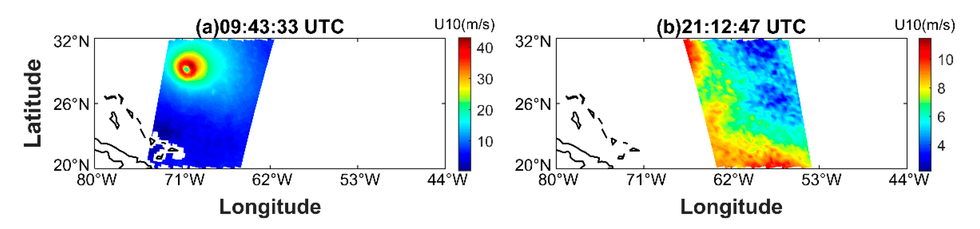
Two observation results for Hurricane Florence acquired by the SMAP radiometer at 09:43 UTC and 21:12 UTC on 12 September 2018, respectively. (a) The observation result contains the complete structure of Hurricane Florence; (b) Hurricane Florence was not observed as it was not covered by the swaths of the SMAP radiometer. Since the observation results obtained by the SMAP radiometer provide a better visualization to analyze the tropical cyclone (TC) position than those acquired by the CYGNSS constellation, these two results were reserved with no further processing.
Figure 6.
Two observation results for Hurricane Florence acquired by the SMAP radiometer at 09:43 UTC and 21:12 UTC on 12 September 2018, respectively. (a) The observation result contains the complete structure of Hurricane Florence; (b) Hurricane Florence was not observed as it was not covered by the swaths of the SMAP radiometer. Since the observation results obtained by the SMAP radiometer provide a better visualization to analyze the tropical cyclone (TC) position than those acquired by the CYGNSS constellation, these two results were reserved with no further processing.

Figure 7.
(a) An observation result for Hurricane Florence acquired by the SMAP radiometer at 20:23 UTC on 11 September 2018. Since this result contains only a fraction of Hurricane Florence, the CYGNSS results from 20:30 to 23:30 UTC (shown in subplot (b)) were used to obtain the complete structure of the TC. The final fusion result is shown in subplot (c).

Figure 8.
Three observation results for Hurricane Florence acquired by the CYGNSS constellation at (a) 13:30 UTC, (b) 14:30 UTC and (c) 15:30 UTC on 9 September 2018. Since it is difficult to fix the center of Hurricane Florence using any of the three results, they were fused to obtain the complete structure of Hurricane Florence. The result of the final fusion is shown in subplot (d).

Figure 9.
The final fusion image of Hurricane Florence observed from 8 to 12 September 2018 using the SMAP radiometer data and the CYGNSS data. (a1)–(a4), (b1)–(b4), (c1)–(c4), (d1)–(d4), and (e1)–(e4) show the daily fusion results from 8 to 12 September 2018, respectively. A black circle with a radius of 150 km was used to mark the location of Hurricane Florence in the fusion image.

Figure 10.
The final fusion image of Hurricane Florence observed from 8 to 12 September 2018 using the CYGNSS data. (a1)–(a3), (b1)–(b3), (c1)–(c3), (d1)–(d3), and (e1)–(e3) show the daily fusion results from 8 to 12 September 2018, respectively. A black circle with a radius of 150 km was used to mark the location of Hurricane Florence in the fusion image.

Figure 11.
Comparison of the estimated and NHC best tracks of Hurricane Florence observed from 8 to 12 September 2018. The track of Hurricane Florence estimated with the geostationary operational environmental satellites (GOES)-16 GeoColor images was also added for comparison.
Figure 11.
Comparison of the estimated and NHC best tracks of Hurricane Florence observed from 8 to 12 September 2018. The track of Hurricane Florence estimated with the geostationary operational environmental satellites (GOES)-16 GeoColor images was also added for comparison.

Figure 12.
Comparison between the estimated maximum wind speeds of Hurricane Florence and the best track peak winds estimated by the NHC from 8 to 12 September 2018.
Figure 12.
Comparison between the estimated maximum wind speeds of Hurricane Florence and the best track peak winds estimated by the NHC from 8 to 12 September 2018.


Table 1.
Comparison between the estimated and NHC best tracks of observed hurricanes.
| Hurricane | Observation Period | Observation Data | MAE (km) | SD (km) | Number of Samples |
|---|---|---|---|---|---|
| Florence | 08 to 12 September 2018 | SMAP + CYGNSS | 38.6 | 28.2 | 14 |
| CYGNSS | 53.7 | 33.8 | 12 | ||
| Dorian | 01 to 04 September 2019 | SMAP + CYGNSS | 30.7 | 15.1 | 13 |
| CYGNSS | 40.1 | 22.7 | 11 | ||
| Michael | 08 to 10 October 2018 | SMAP + CYGNSS | 45.5 | 16.9 | 10 |
| CYGNSS | 49.6 | 23.2 | 8 | ||
| Harvey | 23 to 26 August 2017 | SMAP + CYGNSS | 46.0 | 23.1 | 11 |
| CYGNSS | 54.6 | 28.6 | 9 | ||
| Norman | 30 August to 02 September 2018 | SMAP + CYGNSS | 40.7 | 24.7 | 12 |
| CYGNSS | 50.0 | 26.9 | 9 | ||
| Aletta | 07 to 09 June 2018 | SMAP + CYGNSS | 40.5 | 18.3 | 10 |
| CYGNSS | 47.3 | 27.9 | 7 | ||
| Lane | 20 to 23 August 2018 | SMAP + CYGNSS | 18.4 | 11.6 | 11 |
| CYGNSS | 47.9 | 22.0 | 8 | ||
| Rosa | 27 to 30 September 2018 | SMAP + CYGNSS | 40.5 | 18.9 | 11 |
| CYGNSS | 49.2 | 27.1 | 8 | ||
| Humberto | 16 to 19 September 2019 | SMAP + CYGNSS | 36.7 | 23.3 | 10 |
| CYGNSS | 40.0 | 24.4 | 8 | ||
| Lorenzo | 27 to 29 September 2019 | SMAP + CYGNSS | 38.5 | 20.0 | 10 |
| CYGNSS | 48.7 | 25.9 | 7 |
Table 2.
Comparison between the estimated and NHC maximum wind speeds of observed hurricanes.
| Hurricane | Observation Period | Observation Data | MAE (m/s) | RMSD (m/s) | Correlation Coefficient | Bias (m/s) | Number of Samples |
|---|---|---|---|---|---|---|---|
| Florence | 08 to 12 September 2018 | SMAP + CYGNSS | 13.0 | 15.6 | 0.6031 | 1.5 | 14 |
| CYGNSS | 15.8 | 17.6 | 0.4348 | 2.0 | 12 | ||
| Dorian | 01 to 04 September 2019 | SMAP + CYGNSS | 15.7 | 18.0 | 0.1782 | −3.7 | 13 |
| CYGNSS | 6.4 | 8.8 | 0.8216 | −1.5 | 11 | ||
| Michael | 08 to 10 October 2018 | SMAP + CYGNSS | 15.1 | 16.1 | 0.2496 | 4.5 | 10 |
| CYGNSS | 6.1 | 7.0 | 0.9745 | 1.2 | 8 | ||
| Harvey | 23 to 26 August 2017 | SMAP + CYGNSS | 8.6 | 11.0 | 0.9877 | 1.0 | 11 |
| CYGNSS | 10.0 | 11.9 | 0.9747 | 1.4 | 9 | ||
| Norman | 30 August to 02 September 2018 | SMAP + CYGNSS | 12.2 | 13.4 | 0.7601 | −2.5 | 12 |
| CYGNSS | 12.5 | 13.9 | 0.7423 | −3.0 | 9 | ||
| Aletta | 07 to 09 June 2018 | SMAP + CYGNSS | 10.9 | 12.6 | 0.7385 | −3.3 | 10 |
| CYGNSS | 11.4 | 13.2 | 0.6197 | −4.5 | 7 | ||
| Lane | 20 to 23 August 2018 | SMAP + CYGNSS | 11.3 | 13.4 | 0.3436 | −8.5 | 11 |
| CYGNSS | 12.1 | 14.1 | 0.0572 | −10 | 8 | ||
| Rosa | 27 to 30 September 2018 | SMAP + CYGNSS | 11.6 | 13.1 | 0.5229 | −6.4 | 11 |
| CYGNSS | 12.9 | 13.6 | 0.4040 | −8.9 | 8 | ||
| Humberto | 16 to 19 September 2019 | SMAP + CYGNSS | 7.7 | 8.6 | 0.9034 | −1.8 | 10 |
| CYGNSS | 9.6 | 11.1 | 0.2471 | −8.8 | 8 | ||
| Lorenzo | 27 to 29 September 2019 | SMAP + CYGNSS | 13.3 | 14.7 | 0.6040 | −5.1 | 10 |
| CYGNSS | 15.3 | 16.6 | 0.5603 | −5.7 | 7 |
© 2020 by the authors. Licensee MDPI, Basel, Switzerland. This article is an open access article distributed under the terms and conditions of the Creative Commons Attribution (CC BY) license (http://creativecommons.org/licenses/by/4.0/).
Share and Cite
MDPI and ACS Style
Wang, S.; Shi, S.; Ni, B. Joint Use of Spaceborne Microwave Sensor Data and CYGNSS Data to Observe Tropical Cyclones. Remote Sens. 2020, 12, 3124. https://doi.org/10.3390/rs12193124
AMA Style
Wang S, Shi S, Ni B. Joint Use of Spaceborne Microwave Sensor Data and CYGNSS Data to Observe Tropical Cyclones. Remote Sensing. 2020; 12(19):3124. https://doi.org/10.3390/rs12193124
Chicago/Turabian StyleWang, Shiwei, Shuzhu Shi, and Binbin Ni. 2020. "Joint Use of Spaceborne Microwave Sensor Data and CYGNSS Data to Observe Tropical Cyclones" Remote Sensing 12, no. 19: 3124. https://doi.org/10.3390/rs12193124
Note that from the first issue of 2016, this journal uses article numbers instead of page numbers. See further details here.