

Abstract
We adopt an approach known as bright spots analysis to identify U.S. regions with surprisingly high corn yields given regional expectations, seasonal weather, and soil characteristics. These counties are regional 'surprises' that, by definition, achieve unexpectedly high levels of agricultural productivity. We then use multinomial logistic regression to identify the actionable factors—or the factors over which agricultural stakeholders can exert a certain level of control—that most strongly predict whether a county is a bright spot. We find that farmers in surprisingly productive regions spend an average of $17.6 more per acre on fertilizer, $12.4 more per acre on labor, irrigate 12% more of operated land, and receive $6.6 more per acre from government programs than those cultivating in less productive regions. We conclude by questioning whether and to what extent these attributes of productive regions can be managed for a sustainable future.
Export citation and abstract BibTeX RIS

Original content from this work may be used under the terms of the Creative Commons Attribution 4.0 license. Any further distribution of this work must maintain attribution to the author(s) and the title of the work, journal citation and DOI.
1. Introduction
Nearly 40% of global land is devoted to food production (Ramankutty et al 2008, Foley et al 2011). In the U.S., this number rises to 55%, with two-thirds of all cropland cultivated with corn, wheat, or soy (Bigelow & Bourchers, 2017; USDA Nass 2019). The yields of these crops have climbed consistently in recent decades, thanks largely to technological innovation—particularly genetic improvements (Cooper et al 2014)—and an increased reliance on off-farm inputs (Mulvaney et al 2009, Pimentel and Burgess 2014, Burchfield, Matthews-Pennanen, Schoof, & Lant, 2019). At the same time, real farmer incomes have declined (Mishra and Sandretto 2002, Parton et al 2007), farm debt has increased (Key 2019), and environmental externalities linked to agricultural intensification have grown (Cardinale et al 2012, Tscharntke et al 2012). These challenges will likely be exacerbated by a rapidly changing climate (Schlenker and Roberts 2009, Romero-Lankao et al 2014, Zhao et al 2017) and an estimated doubling of global food demand by 2050 (Ray et al 2013, Valin et al 2014). For agricultural systems to thrive in the future, they must meet human demand while also sustaining the environmental resource base and farmer livelihoods (NRC 2010). The future of agriculture, therefore, lies in identifying the attributes of highly productive agricultural systems and questioning whether and to what extent these attributes can be managed for a sustainable future.
We employ bright spots analysis to locate U.S. counties where the yields of corn—the most widely cultivated crop in the U.S.—are surprisingly higher than expected given regional expectations, seasonal weather, and soil suitability. Unlike traditional outlier analysis, this approach locates regions that deviate strongly from expectations given a set of conditions. These counties are regional 'surprises' that, by definition, achieve unexpectedly high levels of agricultural productivity. We then use multinomial logistic regression to identify the actionable factors—or the factors over which agricultural stakeholders can exert a certain level of control—that most strongly predict whether a county is a bright spot. In surprisingly productive regions, we observe higher rates of fertilizer expense, labor expense, irrigation use, and financial support from federal programs. We conclude by questioning whether and to what extent these correlates of productivity can be managed for a sustainable future.
2. Methods
2.1. Bright spot identification
We generated yield expectations at two spatial scales—the U.S. county and the National Conservation Service's Land Resource Regions (figure 1)—by constructing a null model with random effects at both scales and nonactionable factors known to affect agricultural productivity over which farmers have little control. These nonactionable factors consisted of three indicators of seasonal weather exposure and one soil suitability indicator. The three county-level indicators of seasonal weather exposure—growing degree days (GDDs), stress degree days (SDDs), and total precipitation (TP)—were constructed from gridded daily four-kilometer temperature and precipitation data provided by the PRISM Climate Group for each year included in the analysis. To align daily gridded weather data with county-level yield data, we computed the average daily maximum temperature and precipitation in each county and then summed these daily values for all days in the growing season—defined using the spatially-explicit growing season planting and harvesting dates provided by Ramankutty et al (2008). To compute GDDs—an indicator of cumulative temperature exposure—we summed maximum daily temperatures within a crop-specific tolerance range (10 °C to 30 °C for corn) over the growing season for each county in the coterminous U.S. (Cross and Zuber 1972). To model the effects of heat stress on plant growth (Schlenker and Roberts 2009, Lobell et al 2013, Schauberger et al 2017, Burchfield et al 2019), we also included a metric of seasonal heat exposure called SDDs which measures the total accumulated daily degrees above the maximum GDD threshold temperature (30 °C for corn). To control for the effects of seasonal precipitation on yields, we computed TP, or the sum of precipitation (in millimeters) throughout the growing season.
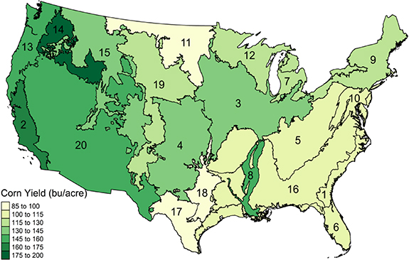
Figure 1. Land Resource Region boundaries and average corn yield (bushels per acre) recorded in USDA Census years between 1997 and 2017. Note that the Florida Subtropical Fruit, Truck Crop, and Range Region (6) and the Northwestern Forest, Forage, and Specialty Crop Region (13) were dropped from the models as less than ten county-year yield observations were available over the period of interest for these regions.
Download figure:
Standard image High-resolution imageIn addition to these seasonal weather indicators, we extracted to the county level an indicator of the suitability of a region's soils to the cultivation of corn provided by the gSSURGO dataset, the highest accuracy and finest spatial resolution dataset available for U.S. soils (Soil Survey Staff 2019). This indicator, the National Commodity Crop Productivity Index (NCCPI), integrates soil chemical properties (e.g. pH, cation exchange capacity, organic matter, adverse chemical properties in the root zone), soil water properties (e.g. available water-holding capacity, precipitation recharge, water table recharge), soil physical properties (e.g. bulk density, soil depth), soil climate properties (e.g. frost-free days, precipitation), soil landscape properties (e.g. slope, depth to water table during growth season), and other soil properties (e.g. surface rock fragments, erosion) to generate a 'corn productivity score' that ranges from 0.01 (low productivity) to 0.99 (high productivity) (Dobos et al 2012). To align this gridded dataset with the county-level yield data, we computed the average productivity score of the subset of only a county's agricultural lands to the cultivation of corn. We measured corn productivity using county-level yield estimates (bushels/acre) provided by the USDA NASS Survey. The final null panel includes only counties reporting more than two years of corn yields (n = 1896 counties) over recent USDA Census year: 1997, 2002, 2007, 2012, and 2017.
Despite the importance of irrigation in explaining yield variability, we did not include it as a predictor in the null model because data suggests that irrigation rates have changed considerably in many counties over the last 20 years. For this reason, we consider irrigation to be an actionable factor and include it in the attribute analysis described below. To test the sensitivity of our results to this assumption, we ran null models including irrigated extent which produced similar seasonal weather response curves and bright and dark spots (SI table 8 available online at stacks.iop.org/ERL/15/104019/mmedia).
Our null model is specified as:


where t indexes time, c indexes counties, and r indexes regions. To account for strong spatial autocorrelation in the county yield data, county-level random effects ( ) are modeled using a Besag-York-Mollie (BYM) spatial dependency model that includes both random effects (
 ) and county-level intrinsic conditional autoregressive (iCAR) structured residuals between counties (
 ). This approach accounts for both random variation in yield across counties and the fact that observations from neighboring counties exhibit higher correlation than more distant regions (Morris et al 2019). The county-level random effects (
 ) capture time-invariant factors associated with a county that influence yield and serve as the basis for our identification of bright spots.
In addition to the county-level effects, we estimated random effects (iid) for each Land Resource Region which define regional yield expectations ( ). We focused on regional expectations rather than national expectations because of the tremendous variability in agricultural system characteristics across the U.S. This approach also allows us to identify the most deviant counties in a region given null model covariates while shrinking counties to the regional means (Gelman and Hill 2007, Cinner et al 2016). We tested the sensitivity of our models to other regional definitions including U.S. state boundaries, U.S. EPA Level II Ecoregions, and national average yield and found the null model using Land Resource Regions to consistently be the best performing model (SI tables 6 and 7).
To capture well-established non-linearities in the effects of seasonal precipitation and temperature on yields (Schlenker and Roberts 2009, Lobell et al 2013), we modeled the interactions between yields and county-year seasonal weather predictors (GDDs, SDDs, TP) using a first-order random walk function,  . This structure allows the effect of these predictors to vary non-linearly while also accounting for autocorrelation in predictors effects. To avoid overfitting, we modeled soil suitability as a county-level linear control,
  . We also included a dummy indicator for year (
 ) to capture any dynamics that affect all counties in a particular year such as major market or policy changes.
The final null model uses uninformative (reduced precision) prior distributions for linear effects and penalized complexity priors for non-linear seasonal weather predictors. The penalized complexity priors employ a scaling factor to specify priors based on reasonable limits of the data (Simpson et al 2014). We employed default and recommended settings for penalized complexity priors as provided by Simpson et al (2014). Model fit was evaluated using the deviance information criterion, the conditional predictive ordinate, the predictive probability integral transform, posterior predictive p-values, mean squared error (MSE) and Bayesian R-squared (R2) (Gelman and Hill 2007, Blangiardo and Cameletti 2015, Gelman et al 2017). All models were estimated using the R-INLA package (Rue et al 2009) in R (R Core Team 2019). Model scripts and additional information on model diagnostics and robustness checks are available at https://github.com/eburchfield/Bright_spots.
Following Cinner et al (2016), we defined bright and dark spots as the counties in which county-scale random effects ( ) differed by more than 1.5 standard deviations from their regional expected value (
 ). For a county
  belonging to a region
  :
:
County-level bright and dark spots are, therefore, counties that, given the null model covariates, deviate from regional yield expectations significantly more or less than other counties deviate from their regional expectations over the five years included in our analysis.
2.2. Bright spot attributes
Though these nonactionable factors strongly influence where and how farmers cultivate different crops, there are many other actionable factors actively managed by humans to create or support desirable cultivation conditions. These include the use of on-farm inputs, participation in federal programs, farm characteristics, and land use decisions (figure 2). Perhaps the most important of these actionable factors are on-farm inputs. Over the period from 1960 to 2018, application rates of synthetic nitrogen fertilizer across the U.S. increased from 17.0 to 83.6 pounds per acre/year (USEPA 2018). Over the same period, pesticide expenditures experienced a fivefold increase, with recent annual U.S. expenditures over $12 billion (Fernandez-Cornejo et al 2014). Corn has been the top pesticide-using crop in the U.S. since the 1970s; today, over 90% of U.S. corn is treated with pesticides (Fernandez-Cornejo et al 2014). Irrigation is another crucial input to production, with irrigated land in the U.S. increasing from 37 million acres in the 1960s to 55.9 million acres in 2018. Today, irrigated acreage comprises 28% of all harvested cropland and generates roughly half of the total value of U.S. crop sales (USDA ERS 2019). Over the last century, farms have also become far less reliant on physical labor as an input to production, largely due to the rapid advances in mechanization (Mazoyer and Roudart 2017). On-farm labor has decreased from 9.93 million farmworkers in 1950 to 2.31 million farmworkers in 2019 (USDA ERSa 2020; USBLS, 2019). Financial support for agricultural production through direct payments from federal programs to farmers has also increased in recent decades (Annan and Schlenker 2015), providing an important source of income stabilization and financial incentive for retiring land from production for many farmers.In addition to on-farm inputs and financial support, farm characteristics influence the on-farm adoption of new technologies and practices that influence agricultural yields. For example, research suggests that the adoption of agricultural best management practices increases as farmer age decreases (Prokopy et al 2008), rates of tenancy decrease (Soule et al 2000), and access to education and extension increase (Baumgart-Getz et al 2012); however, the direction of these effects is not always clear, and often contradictory across analyses (Knowler and Bradshaw 2007). Though farmer characteristics such as age and gender are not directly actionable by farmers, policies and programs can target specific groups of farmers to increase access to information or to support their production.
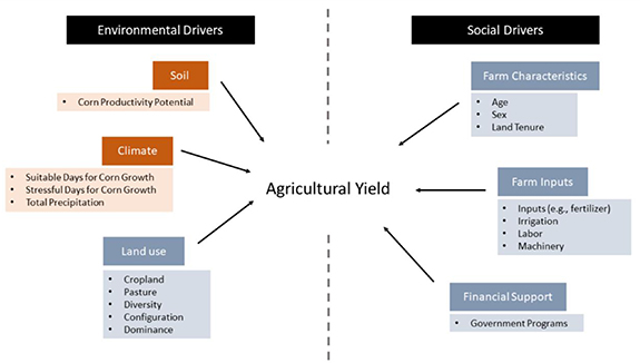
Figure 2. Environmental and social correlates of agricultural production. Correlates deemed nonactionable are shown in orange; actionable correlates are shown in blue.
Download figure:
Standard image High-resolution imageFinally, changes in land use can alter the provisioning of ecosystem services essential to agricultural production (Shackelford et al 2013, Duarte et al 2018). Increased configurational and compositional complexity of an agricultural landscape is associated with greater pollinator movement and plant reproduction (Hass et al, 2018; Garibaldi et al 2011), bird and arthropod diversity (Fahrig et al 2015, Sirami et al 2019), water quality (Gergel et al 2002), and higher yields (Burchfield et al 2019). Though individual farmers may not have the capacity to manage these landscape dynamics, shifts in regional agricultural policy and markets can shape the crops that are cultivated and the ways in which land is managed (Boody et al 2005); therefore, we designate these landscape characteristics as actionable.
To assess the contribution of these actionable factors to agricultural production, we constructed a panel dataset describing the agricultural and land use characteristics of corn-producing counties in the coterminous U.S. in recent USDA Census years (1997, 2002, 2007, 2012, 2017). The USDA Agricultural Census is administered every five years to all farms and ranches selling at least $1000 of their products and is the only source of detailed county-level U.S. agricultural data that is collected, tabulated, and published using a consistent methodology that covers the coterminous U.S. Our analyses are limited to the actionable factors for which more than 80% of data was available for the county-years of interest. This excluded interesting variables (e.g. crop insurance payments and on-farm experience), but was necessary for modeling purposes. The final set of predictors we compiled from the USDA Census included available data describing farm and farmer characteristics (age, sex, and land tenure), farm inputs (fertilizer expense,1 labor expense, and machinery costs), financial support (direct receipts from federal programs), and land use (percent agricultural land in corn production, percent county land in pasture or cropland) (figure 2). Given the growing body of literature indicating that shifts in land use can affect agricultural productivity, largely through the provisioning of ecosystem services, we also constructed additional indicators of land use from the USDA Cropland Data Layer–a 30-meter annual land use dataset based on satellite imagery and extensive ground truth data. In addition to the compositional indicators extracted from the USDA Census, we constructed indicators of land use diversity (Richness, or the number of distinct land use categories in a county) and dominance (Largest Patch Index, or the percent of the total landscape covered by the largest patch in the county). We focus on these indicators of composition to contribute to debates in the literature on the role of landscape specialization to agricultural productivity (Abson et al 2013, Davis et al 2012; Hass et al, 2018, Landis 2017). Our previous research also indicates that high levels of land use diversity are associated with high yields of corn, wheat, and soy (Burchfield et al 2019), which challenges the association between specialized and simplified landscapes and productivity (Key 2019). In addition to these indicators of landscape composition (percent corn, percent cropland, percent pasture, richness, and largest patch index), we also include two commonly used indicators of landscape configuration: an indicator of the distribution of different land use categories across a landscape (Interspersion and Juxtaposition Index) and an indicator of the patchiness of a landscape (Edge Density). Managing for configurational complexity, where fine-grained agricultural landscapes are well connected to surrounding habitats, has been shown to enhance natural enemies (Haan et al 2020) and increase yields in conventional systems (Martin et al 2016).
We used multinomial logistic regressions to estimate the effect of predictors on a county's membership in the bright or dark spot categories as compared to the average category. This approach allows the predictors to affect membership in each category differently. While this exploratory approach does not imply that these correlates have a direct and causal effect on yield, it does provide an indication of the characteristics typical of highly productive regions, allowing us to identify the characteristics of places that defy expectations and to discuss whether and to what extent these attributes can be managed for a sustainable future.
The analysis was performed in R using the nnet package (Venables and Ripley 2002) to compute the log-odds of a county in the average reference category changing membership to either a bright or dark spot category as a function of farm characteristics, farm inputs, and land use. We standardized predictors (where applicable) to facilitate comparison across counties using 'total operated acres' which includes agricultural land used for crops, pasture, or grazing, as well as woodlands, farm roads, and farm buildings (USDA NASS 2019). All covariates included in the final models had correlation coefficients less than 0.7 and variance inflation factor scores less than 5.
3. Results
Our model identifies 109 bright spots clustered in the heart of the Corn Belt, in southwestern Georgia, in the Texas Panhandle, and along the Lower Mississippi (figure 3; SI table 9). These are counties whose corn yields—as compared to regional expectations—are unexpectedly high (bright spot) or low (dark spot). Bright spots are clustered in the heart of the Corn Belt in western Illinois and parts of Iowa, as well as in southwestern Georgia, around the Oklahoma Panhandle, and along the Mississippi River in Arkansas and Louisiana. Dark spots are found along the periphery of the Corn Belt—in southeastern Kansas through northern Missouri, northern Michigan, and across the Dakotas. We also see a cluster of dark spots in northern Michigan and in central Virginia—areas where relatively little corn is grown (figure 3; SI table 10).

Figure 3. Location of 109 bright spots (green) and 108 dark spots (blue) derived from the hierarchical model.
Download figure:
Standard image High-resolution imageTable 2 presents the regression coefficients for fixed effects in the hierarchical model. These results indicate that the majority of U.S. corn yield variability is explained by differences in soil and climate (R2 of 0.72; SI tables 3 and 4). For example, a one standard deviation increase in soil suitability is associated with a corn yield increase 12.4 bu ac–1 (table 2). A one standard deviation increase in seasonal GDD exposure from average exposure rates (approximately 580 GDDs) is associated with a yield increase of 25 bu ac−1 (figure 4(a)), while increased exposure to seasonal temperature stress of 150 stress degree days is associated with a decrease in yields of 15 bu ac−1 (figure 4(b)). Corn yields are less responsive to changes in total precipitation (figure 4(c)), which reflects the importance of irrigation in mitigating the effects of precipitation variability on corn production (Cooper et al 2020). These results correspond with existing research finding that seasonal weather variability explains up to 70% of yield variability (Ray et al 2012, 2015, Liang et al 2017), that corn yields drop sharply when temperatures exceed 30 °C (Schlenker and Roberts 2009, Lobell et al 2013, Schauberger et al 2017, Messina et al 2019), and that soil suitability is a major determinant of productivity (Kravchenko and Bullock 2000).
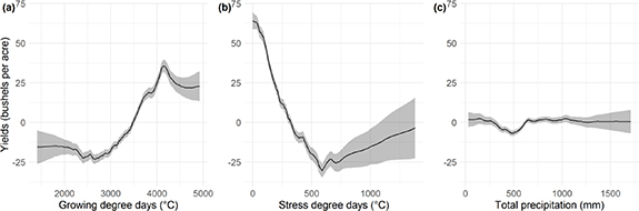
Figure 4. The non-linear response (first-order random walk) of corn yields (bushels per acre) to seasonal weather covariates in the hierarchical model. Solid lines show the median effect and shaded bands the 95% credibility limits.
Download figure:
Standard image High-resolution imageTable 1. Variable descriptions.
| Variable | Description and measurement |
|---|---|
| Hierarchical model predictors | |
| Soil suitability | National Commodity Crop Productivity Index (NCCPI) from the gSSURGO dataset (USDA NRCS Soil Survey Staff, Natural Resources Conservation Service 2019). |
| Growing degree days | Cumulative seasonal exposure to temperatures beneficial to corn production (between 10 and 30 ˚C). |
| Stress degree days | Cumulative seasonal exposure to temperatures detrimental to corn production (above 30 ˚C). |
| Total precipitation | Cumulative seasonal precipitation in millimeters. |
| Farm characteristics | |
| Age | Average age of primary producer; measured as average years across a county's primary producers. |
| % females | Percentage of agricultural acres operated by female primary producers; measured as the number of agricultural acres operated by female primary producers and standardized by the total number of agricultural acres operated, per county. |
| % owners | Percentage of agricultural acres operated by full owners (producers who operate only land they own); measured as the number of agricultural acres operated by full owners and standardized by the total number of agricultural acres operated, per county. |
| % tenants | Percentage of agricultural acres operated by tenants (producers who operate land they rent from others and/or land they worked on shares for others); measured as the number of agricultural acres operated by tenants and standardized by the total number of agricultural acres operated, per county. % partial owners not included in the model. |
| Farm inputs | |
| Fertilizer | Total expense of fertilizers, including lime and soil conditioners, rock phosphate and gypsum, and the cost of custom application, per agricultural acre; measured as total expense in USD $ and standardized by the total number of agricultural acres operated, per county. |
| Irrigation | Percentage of agricultural land in every county utilizing irrigation (includes all land irrigated by artificial/controlled means, including lagoon wastewater distributed by sprinkler or flood system); measured as the number of agricultural acres irrigated and standardized by the total number of agricultural acres operated, per county. |
| Labor | Total expense of all laborers, per agricultural acre; measured as the total expense of laborers (hired, contract, and migrant) in USD $ and standardized by the total number of agricultural acres operated, per county. |
| Machinery | Total asset value of agricultural machinery, per agricultural acre; measured as total machinery assets in USD $ and standardized by the total number of agricultural acres operated, per county. |
| Financial Support | |
| Gvt. Receipts | Total cash receipts of government programs, per agricultural acre; measured in USD $ and standardized by the total number of agricultural acres operated, per county.a |
| Land use | |
| % corn | Percentage of total harvested acres in corn; measured as total harvested corn acres and standardized by total harvested cropland acres. |
| % cropland | Percentage of land in a county dedicated to cropland; measured as total acres cropland (includes crop failure, cultivated summer fallow, idle land, harvested cropland, and cropland used only for pasture) and standardized by the total number of acres in a county. |
| % pasture | Percentage of land in a county dedicated to pasture; measured as total acres pasture (excluding pastured cropland) and standardized by the total number of acres in a county. |
| Edge density | A measure of landscape configuration; measured as the sum of all edges (in meters per hectare) of a given class in relation to the landscape area. ED equals 0 if only one patch is present and increases, without limit, as the landscape becomes patchier (Mcgarigal et al 2012). |
| Largest patch index | A measure of landscape dominance; measured as the percentage of the total landscape covered by the largest patch of the corresponding patch type. LPI approaches 0 when the largest patch is small and equals 100 when only one patch-class is present (Mcgarigal and Marks 1995; Mcgarigal et al 2012). |
| Interspersion & Juxtaposition | A measure of landscape aggregation and distribution; measured as a percentage of the maximum possible. IJI ranges from 0 when a patch type is adjacent to only one other patch-class (patch types are poorly interspersed/there is a disproportionate distribution of patch type adjacencies) and 100 when a patch is adjacent to all patch-class types (patch types are well interspersed/equally adjacent to each other) (Mcgarigal and Marks 1995; Mcgarigal et al 2012). |
| Richness | A measure of landscape diversity; measured as the number of unique land use categories in a county. Richness approaches 1 when only one patch is present in a large landscape and increases, without limit, as the number of unique land uses increases, and the landscape area decreases (Mcgarigal et al 2012). |
aThis category consists of direct payments from the government and includes: payments from Conservation Reserve Program, Wetlands Reserve Program, Farmable Wetlands Program, and Conservation Reserve Enhancement Program; loan deficiency payments; disaster payments; other conservation programs; and all other federal farm programs under which payments were made directly to farm operators. Commodity Credit Corporation (CCC) proceeds, local and state government agricultural program payments, and federal crop insurance payments are not tabulated in this category (USDA NASS 2019, p. 759).
Table 2. Regression coefficients for fixed effects in the hierarchical model. Soil suitability was standardized prior to analysis, so the effect reported below is based on a one standard deviation increase in soil suitability. The baseline year in the model is 1997.
| Variable | Mean | St. Dev. | 0.025 quantile | 0.975 quantile |
|---|---|---|---|---|
| Intercept | 96.83 | 9.34 | 78.49 | 115.16 |
| Soil suitability | 12.37 | 0.76 | 10.88 | 13.86 |
| Year 2002 | 6.35 | 0.70 | 4.97 | 7.72 |
| Year 2007 | 22.31 | 0.71 | 20.92 | 23.70 |
| Year 2012 | 21.42 | 0.75 | 19.95 | 22.90 |
| Year 2017 | 43.65 | 0.68 | 42.33 | 44.98 |
We predict membership in one of three categories (bright, average, or dark) using the variables described in table 1 with multinomial logistic regression analysis. Our model performs well on held-out data, correctly predicting 89% of the cases (n = 8650 county-years, McFadden's pseudo R2 0.23). Results are robust to shifts in the threshold we used to define bright spots (SI figures 4 and 5). Predictors were scaled prior to analysis, so the effects presented in figure 5 and table 3 are the relative risk ratios associated with a one standard deviation increase in each covariate. Keeping all other variables constant, variables with relative risk ratios less than one are more likely to shift towards the average category as the value of the variable increases; conversely, variables with relative risk ratios greater than one are more likely to shift to the bright (figure 5(a)) or dark (figure 5(b)) categories as the value of the variable increases. In what follows, we focus on the attributes with relative risk ratios greater than one, as these attributes are most likely to push a county out of the average category towards classification as a bright or dark spot.

Figure 5. Relative risk ratios associated with a county moving from (a) average to bright or from (b) average to dark. Points are the risk ratios associated with membership in bright or dark spot categories as compared to the baseline average category and lines represent the 95% confidence intervals for these estimates. Keeping all other variables constant, variables with relative risk ratios greater than one are more likely to shift to the bright (figure 5(a)) or dark (figure 5(b)) categories as the variable increases, while variables with relative risk ratios less than one are more likely to shift towards the average category as the variable increases.
Download figure:
Standard image High-resolution imageTable 3. Multinomial logistic regression results presented as relative risk ratios. Our model performs well on held-out data, correctly predicting 89% of the cases (n = 8650 county-years, McFadden's pseudo R2 of 0.23). Predictors were scaled prior to analysis, so the effects presented are the relative risk ratios associated with a one standard deviation increase in each covariate (see SI table 2 for descriptive statistics).
| Dependent variable | ||
|---|---|---|
| Bright | Dark | |
| Farm characteristics | ||
| Age | 1.083 | 0.938 |
| (0.081) | (0.079) | |
| % females | 0.998 | 0.962 |
| (0.071) | (0.071) | |
| % owners | 1.019 | 0.671*** |
| (0.104) | (0.073) | |
| % tenants | 1.117* | 0.545*** |
| (0.073) | (0.066) | |
| Farm inputs | ||
| Fertilizer ($/acre) | 1.346*** | 0.820 |
| (0.133) | (0.124) | |
| Irrigation (%) | 1.393*** | 0.739* |
| (0.075) | (0.114) | |
| Labor ($/acre) | 1.139** | 0.967 |
| (0.069) | (0.100) | |
| Machinery ($/acre) | 0.536*** | 1.162 |
| (0.068) | (0.140) | |
| Financial Support | ||
| Gvt. programs ($/operation) | 1.235*** | 1.033 |
| (0.090) | (0.105) | |
| Land use | ||
| % corn | 1.310*** | 0.408*** |
| (0.092) | (0.041) | |
| % cropland | 0.652*** | 0.732** |
| (0.076) | (0.091) | |
| % pasture | 1.046 | 1.011 |
| (0.091) | (0.090) | |
| Landscape | ||
| Edge density | 0.964 | 0.780** |
| (0.104) | (0.082) | |
| Largest patch index | 0.914 | 0.730*** |
| (0.086) | (0.064) | |
| Interspersion & juxtaposition | 1.226*** | 1.082 |
| (0.094) | (0.081) | |
| Richness | 0.717*** | 0.963 |
| (0.055) | (0.090) | |
| Constant | 0.052*** | 0.035*** |
| (0.004) | (0.003) | |
Note:*p < 0.1,**p < 0.05,***p < 0.01
The results of the multinomial logistic regression indicate that, after controlling for regional expectations, seasonal weather, and soil suitability, unexpectedly high yields are found in regions with higher levels of farm inputs (fertilizer, irrigation, labor) and financial support (government receipts) to production. For example, a one standard deviation increase in dollars spent on fertilizer ($26.34 per acre) is associated with an increase in the likelihood of a county being classified as bright by 35%. Increasing irrigated acreage by 13% increases the likelihood of a county being classified as bright by nearly 40%. A one standard deviation increase in dollars spent on labor ($73.01 per acre) or dollars received from government programs ($8.58 per acre) increases the likelihood of a county being classified as bright by 14% and 23% respectively. Surprisingly, as the asset value of machinery per acre increases, a county is more likely to be classified as average as compared to bright. Changes in land use have a mixed effect on the likelihood of a county being classified as bright. First, our findings suggest that surprisingly productive agricultural regions are also those with higher levels of land use specialization. Bright counties are associated with a higher percent of acres cultivated with corn (% corn) and lower levels of land use diversity (Richness), counter to findings by Burchfield et al (2019) that high levels of diversity are associated with higher corn yields. A county is also less likely to be classified as dark if it is dominated by a single land use category (Largest Patch Index). While compositional diversity may not be associated with surprisingly productive regions, we find that as there is a greater distribution of land use categories in a landscape, i.e. a higher probability that different land use categories will be located close to one another (IJI), counties are more likely to be classified as bright. This may imply that it is not total land use diversity (Richness), but the mixing of diverse land use categories across the landscape that is associated with higher yielding regions. This is also supported by the finding that increased landscape patchiness (Edge Density) decreases the likelihood of a county being classified as dark. Finally, farmer characteristics (age, sex) do not have a clear effect on the likelihood of a county being classified as bright, suggesting that what a farmer does matters more than who a farmer is.
4. Discussion
While unsurprising (see for example, Liang et al 2017, Ray et al 2015, or Lobell and Gourdji 2012), our finding that seasonal weather and soil explain much of the variability in U.S. corn production highlights the role that nonactionable factors play in driving yield variability. Though seasonal weather and soil did not show significant changes over our period of interest (SI figure 1), these nonactionable factors are likely to change in the future as climate change brings more frequent extreme heat events, daily precipitation extremes, and more intense droughts over most of North America (Romero-Lankao et al 2014) and as agricultural mismanagement exacerbates soil quality declines already observed across many regions of the U.S. (Stavi and Lal 2015). While many regions stand to benefit from these changes, particularly the warming of the northern U.S. (Lant et al 2016, Burchfield et al 2019), these changes in soil and climate will alter where and how we grow corn in the future, with profound implications for agricultural livelihoods (Sleeter et al 2012, Sohl et al 2012, Lant et al 2016). Given these probable changes in climate and soil, we have conducted exploratory analyses to identify the attributes of U.S. counties that have shown surprisingly high levels of productivity in recent years. While our analyses are correlative not causal, they provide preliminary evidence for the management practices, farm characteristics, and land use contexts associated with U.S. counties that have achieved surprisingly high yields—given local climate and soil dynamics—allowing us to discuss the extent to which these correlates of productivity can continue to be managed for a sustainable future.
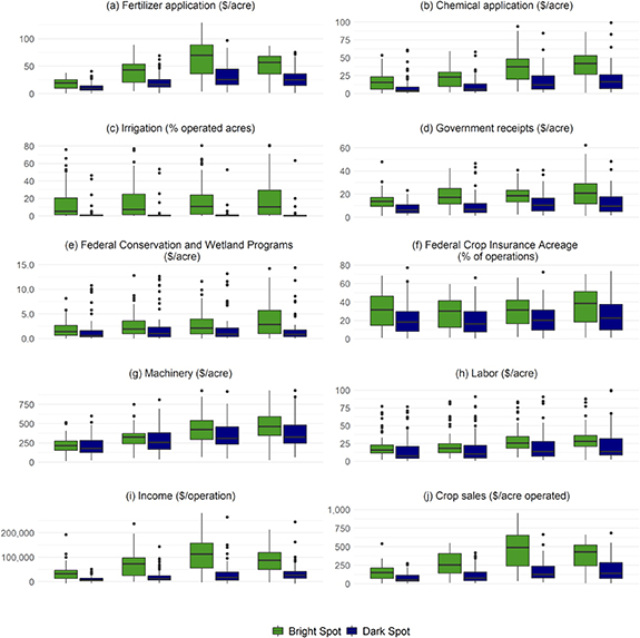
One of the strongest predictors of whether a county is classified as bright is fertilizer use. Over the years included in our analysis, farmers cultivating in bright counties spent an average of $38.5 per acre on fertilizer as compared to $20.9 per acre in dark counties (figure 6(a)). Chemical application—though not included in our analysis due to its high collinearity with fertilizer use—is also consistently higher in bright counties, with average spending of $26.2 per acre in bright counties as compared to $13.1 in dark counties (figure 6(b)). Farmers in bright counties also have greater machinery assets (figure 6(g)) and spend more on labor (figure 6(h)). Mechanical technology innovations have contributed widely to agricultural productivity in the U.S., significantly reducing the need for on-farm labor (USDA ERSa 2020). At the same time, the supply of farm labor has declined and the cost of labor increased, encouraging farmers to grow less labor-intensive crops while investing in labor-saving technologies and increasing labor productivity (Zahniser et al 2018). Given our findings that investing more in labor increases the likelihood of a county being classified as bright and investing more in machinery makes a county more likely to be classified as average as compared to bright, we suggest that more research investigating the nuanced links and feedbacks between labor, machinery, and productivity is necessary in the future. Finally, many of the counties with surprisingly high corn yields also have high rates of irrigation, with an average irrigation rate of 14.7% in bright counties as compared to only 2.6% in dark counties (figure 6(c)).
Figure 6. Box and whisker plot showing differences in physical and financial inputs across bright spots and dark spots. Bold horizontal lines represent the median. We include an indicator of chemical application (insecticides, herbicides, fungicides, pesticides, and the cost of application) not included in the formal analysis due to high collinearity with fertilizer use. We also include indicators of participation in specific government programs excluded from formal analysis due to limited data availability over our period of study. Due to data availability issues, 1997 was not included in these figures.
Download figure:
Standard image High-resolution image
Whether these high rates of input use can mitigate projected changes in climate and soil is unclear. On the one hand, these are important means of replicating ideal cultivation conditions in regions that are not particularly well-suited to the cultivation of a specific crop. On the other hand, there are significant environmental implications of this reliance on external inputs, particularly their negative influence on the nonactionable factors—soil suitability and climate—that drive much of yield variability in the U.S. For example, though fertilizer application is an important means of boosting agricultural productivity, its overuse is associated with a number of social and environmental externalities including eutrophication and hypoxia (Van Meter et al 2018), biodiversity loss (Mozumder and Berrens 2007), soil chemical and biological degradation (Mulvaney et al 2009, Stavi and Lal 2015), and human infections and diseases (Horrigan et al 2002). Of particular concern is the contribution of increased fertilizer use to global emissions of nitrous oxide (N2O), a greenhouse gas whose global warming potential is nearly 300 times that of CO2 (Davidson 2009, Park et al 2012, Fu et al 2017). These emissions exacerbate global climate change, further deteriorating the climatic conditions on which successful corn cultivation depends (Pinder et al 2012). Similarly, irrigation allows agricultural systems to achieve higher yields than could be supported by the natural environment alone; however, in many regions, irrigation rates are rapidly exceeding sustainable limits, raising questions about their capacity to continue to support high levels of productivity into the future. For example, the bright counties in the Texas Panhandle withdraw groundwater from the Ogallala Aquifer, in which up to 24% of irrigated area may be lost this century (Deines et al 2019). The cluster of bright counties in eastern Arkansas—a region that has seen a remarkable expansion of irrigated area in recent decades—withdraws from an aquifer currently classified as 'critical' due to significant groundwater declines and water quality degradation (Vories and Evett 2014). In the Lower Mississippi River Valley—where we find a large concentration of bright spots—aquifer levels have declined by an average of 370 million cubic meters per year over the last 25 years (Kebede et al 2014). Both the Southeast and the Midsouth are expected to see an increase in the prevalence and severity of drought in the future, exacerbating water stress in these regions (Mearns et al 2003, Strzepek et al 2010).
In addition to the environmental implications of high input use, increased use of inputs may also have implications for agricultural livelihoods. Per farm average expenditures reached over $176 000 in 2017; labor, machinery, fertilizer, and chemicals together comprise over 30% of these expenses (USDA NASS 2018). Over the period covered in this study, farmer debt also increased by 60% from $241 billion (inflation adjusted USD$) in 1997 to $390 billion in 2017—levels not seen since the 1980s farm crisis (USDA ERSc 2020). Over the same period, median farm income has declined, with 2019 net farm income nearly 36% below its peak of $136.5 billion in 2013 (USDA ERSb 2020). While our data shows that farmers in bright counties earn more in terms of income and crop sales than those cultivating in dark counties (figures 6(i)–(j)), we do not have data describing differences in farmer debt across these two groups. In addition, more farmers cultivated as tenants in bright counties than in dark. Given that bright spots are defined by high corn yields, the higher rates of tenancy emphasize the need to understand landowner-tenant relationships and on-farm decision-making (Perry-Hill and Prokopy 2014, Ulrich-Schad et al 2016, Ranjan et al 2019). If, for example, land renters are more concerned about short-term profitability than long-term land value, and are tasked almost exclusively with management decision-making, renters may prioritize high yields at the expense of the long-term sustainability of the lands they lease (Rogers 1991, Soule et al 2000).
Based on these results and the literature on the potential environmental and livelihood impacts of mismanagement of these inputs, we argue that one of the most important areas for sustainable change in U.S. corn production is to increase the efficiency with which current inputs, particularly fertilizer and irrigation water, are applied. Though agricultural total factor productivity (TFP) growth has been significant over the last decades, gains have been biased by technologies that are land- and labor-saving, but input-intensive (Coomes et al 2019; USDA ERSd 2020). Though results from this study cannot speak to input-use efficiency directly, it remains that agricultural inputs are often not applied efficiently. For instance, an estimated 65% of farming operations do not follow best management practices for fertilizer application (Ribaudo et al 2011), with fertilizer often applied in excess of crop requirements (Ladha et al 2005). This decreases soil productivity over time, increasing farmer reliance on synthetic fertilizers (Mulvaney et al 2009). Similarly, in many of the water-stressed aquifers that supply irrigation water to bright spots, water is applied inefficiently, further depleting water supplies and raising energy costs for producers (Kebede et al 2014). Significant efficiency gains can be made by promoting information-intensive—rather than input-intensive—innovations in U.S. agriculture (Fuglie 2018, Burchfield et al 2020). Advances in precision agriculture including the use of Global Positioning Systems, weather prediction, satellite imagery, and drones to target inputs like fertilizer, pesticides, and irrigation water can significantly increase resource use efficiency (Bongiovanni and Lowenberg-Deboer 2004). Genetic innovations designed to mitigate climate, soil, and pest variability have already generated significant efficiency gains (Tester and Langridge 2010, Cooper et al 2014, Khatodia et al 2016, Mueller et al 2019, Messina et al 2020). These innovations in technology, coupled with ecosystem-based approaches (e.g. crop rotation, integrated crop-livestock systems) to TFP growth, have the potential to enhance agricultural sustainability (Coomes et al 2019).
In addition to higher rates of input use, we also find that farmers cultivating in bright counties receive nearly double the government receipts as those cultivating in dark counties ($15.5 per acre versus $8.9 per acre respectively). This variable includes payments for farmer participation in conservation programs, loan deficiency payments, disaster payments and 'all other federal farm programs under which payments were made directly to farm operators' (USDA NASS 2019, p. 759). Due to high rates of missing data, we were unable to formally assess the interactions between farmer participation in specific programs and corn productivity; however, we compare available data across bright and dark counties in figures 6(d)–(f). Participation in federal crop insurance programs has increased consistently through time, reflecting national trends (Annan and Schlenker 2015)—with higher participation rates in bright counties than dark counties. Federal programs are an important source of income stabilization for U.S. farmers; however, participation in these programs is governed by policies that often promote specialization, influencing what, where, and how food is produced (Reganold et al 2011) with implications for farm-level adaptive capacity and resource use. For example, an increased participation in federal crop insurance programs is associated with a decrease in adoption of adaptive practices meant to mitigate the negative yield impacts of changing climate (Annan and Schlenker 2015), reduced on-farm diversification (Di Falco and Perrings 2005, O'Donoghue et al 2009), the cultivation of more water-intensive crops (Deryugina and Konar 2017), and the expansion of corn production into regions poorly suited to its cultivation (Olson 2001, Mcgranahan et al 2013). Though participation in federal conservation and wetland programs is low, the higher rates of participation in bright counties merit further exploration. In addition to preserving important ecosystems, participation in these programs has been shown to boost ecosystem services for agriculture while supplementing farmer income (Gleason et al 2008, Morefield et al 2016).
Changes in land use have a mixed effect on the likelihood of a county being classified as bright. Our results indicate that surprisingly productive regions are those with higher levels of land use specialization (lower Richness, higher percent cultivated in corn, lower Largest Patch Index). At the same time, however, we find that counties with more complex configurations (higher edge density, higher Interspersion and Juxtaposition) are more likely to be bright or average as compared to dark. The different ways in which landscape composition and configuration interact with yield suggest that there may be ways in which agricultural stakeholders can manage entire landscapes to support agricultural production. This aligns with published research suggesting that managing agricultural lands to support the provisioning of ecosystem services essential to agricultural production can increase both ecosystem health and yields (Shackelford et al 2013, Duarte et al 2018); however, more research is needed to assess the specific ways in which shifting land use affects production and input use (Burchfield et al 2019). We note, additionally, that there are many well-established agricultural practices farmers can employ to manage for ecosystem services that we were unable to include in our analysis due to limited data availability. For example, setting aside even a small portion of agricultural land to natural cover has been found to boost ecosystem services essential to agricultural production (e.g. increased pollinator abundance, improving water quality, and controlling soil erosion) while maintaining yields (Schulte et al 2017). Agricultural practices like this, that both maintain yields and promote environmental outcomes, must be included in future analyses (once data is available at U.S. scales) to further understand sustainability as it relates to management practices and agricultural outcomes (e.g. yields) in the U.S.
5. Conclusion
For our food production systems to thrive in the future, they must meet human demand while also sustaining the environmental resource base and providing economically viable options for farmers (NRC 2010). We have identified surprisingly productive regions of the U.S., identified the shared attributes of these regions, and questioned the overall sustainability of these attributes. Rather than identifying the highest or lowest yielding places in the U.S., we identify places that defy expectations to uncover potential actionable levers to boost agricultural sustainability. This exploratory hypothesis-generating expedition both highlights the extent to which nonactionable climatic and edaphic factors explain yield variability and identifies the major correlates of productivity: high levels of input use, land use specialization, and government support. These correlates, in turn, affect the environmental conditions that ultimately define agricultural productivity.
We conclude by emphasizing the importance of future work exploring agricultural bright spots to generate novel insights and new hypotheses about sustainable solutions to the complex problems facing U.S. agriculture (Bennet et al 2016). We propose future research in bright counties where relatively few inputs are used. Bright areas reporting low rates of fertilizer use—located primarily in Texas and Oklahoma (SI figure 6)—and low irrigation rates—located in western Illinois, parts of the Great Plains, and throughout Texas (SI figure 7)—are areas that achieve surprisingly high yields without heavy use of fertilizer and irrigation water. Future research in these areas can merge the 'big data' presented in this analysis with 'deep data' describing the intersecting social and ecological dynamics that allow farmers to achieve high yields in surprising contexts.
Acknowledgments
This article was supported by the Utah Agricultural Experiment Station [UTA01422]. Any opinions, findings, and conclusions or recommendations expressed in this material are those of the author(s) and do not necessarily reflect the views of Utah State University. Many thanks to Ms. Kaitlyn Spangler, Dr. Kate Nelson, and Dr. Martin Van der Linden for constructive and insightful reviews.
Data availability statement
The data that support the findings of this study are available upon reasonable request from the authors.
Author contributions:
Both authors contributed to the data construction, analysis, and writing of the paper. Dr. Burchfield led the analysis and writing of the paper, while Ms. Schumacher led the data construction.
Significance Statement:
Corn is the most important crop to the U.S. economy in terms of revenue and acreage. We find that high corn yields are explained mostly by a serendipitous intersection of good weather and good soil. In regions of surprisingly high yields, we observe high rates of fertilization expense, irrigation use, labor expense, and receipts from government programs. We discuss whether and how these correlates of high productivity can be managed for a sustainable future.
Footnotes
- 1
We initially included both an indicator of fertilizer and chemical use but found the two predictors to be collinear at 0.78, suggesting that farmers who apply fertilizer are also highly likely to apply chemicals (insecticides, herbicides, fungicides, and other pesticides). We tested model sensitivity to inclusion of both predictors and found the effect size and direction of the predictor to be similar across models, so we have only included fertilizer use in the final model.