Noise power spectral density scaled SNR response estimation with restricted range search for sound source localisation using unmanned aerial vehicles

Abstract

A method to locate sound sources using an audio recording system mounted on an unmanned aerial vehicle (UAV) is proposed. The method introduces extension algorithms to apply on top of a baseline approach, which performs localisation by estimating the peak signal-to-noise ratio (SNR) response in the time-frequency and angular spectra with the time difference of arrival information. The proposed extensions include a noise reduction and a post-processing algorithm to address the challenges in a UAV setting. The noise reduction algorithm reduces influences of UAV rotor noise on localisation performance, by scaling the SNR response using power spectral density of the UAV rotor noise, estimated using a denoising autoencoder. For the source tracking problem, an angular spectral range restricted peak search and link post-processing algorithm is also proposed to filter out incorrect location estimates along the localisation path. Experimental results show the proposed extensions yielded improvements in locating the target sound source correctly, with a 0.0064–0.175 decrease in mean haversine distance error across various UAV operating scenarios. The proposed method also shows a reduction in unexpected location estimations, with a 0.0037–0.185 decrease in the 0.75 quartile haversine distance error.

1 Introduction

Unmanned aerial vehicles (UAVs) have recently gained huge popularity over a wide range of applications, such as filming [2], search and rescue [3], or security and surveillance [4]. One of the significant advantages of UAVs is its flexibility in manoeuvrability, allowing ease of navigation through environments that are difficult or dangerous for human access. In the application of search and rescue, there are already several reports of successful rescue missions where victims were found stranded in environments that are difficult to navigate through [5–7]. The key to its success is the use of localisation technologies to track down the whereabouts of the stranded victims effectively. To this day, various sensing technologies were utilised for search and rescue purposes such as high-resolution cameras or thermal imaging. While such sensing technologies are well-proven and highly effective under many types of environments, information from sound is also one that should not be overlooked, for it is common to encounter scenarios where the environment renders visual information as unusable. For example, for a UAV hovering over a mountain range, where vegetation could hinder the visibility of a rescue target, the target could be detected and located by sound. With localisation being the key objective to perform the search and rescue task properly, it is vital that the utilised sensing technologies are effective under a wide range of environments [8], including adverse environments such as those where visual information is severely impaired. In turn, when one method is rendered unusable, others still remain effective. However, audio recording using UAVs has shown to be challenging due to the high noise levels radiated from the UAV rotors. This significantly affects the quality of the audio signals to aid not only with search and rescue, but also with any applications [9–12].

In recent years, numerous studies attempt to perform localisation of sound sources using UAVs. Many achieve this by utilising signal processing techniques that revolve around the usage of an array of microphones [13]. With the significant contamination of recordings caused by rotor noise being a problem, numerous studies attempt to eliminate the effects of rotor noise itself. Examples include denoising the input signals by forming a reference rotor noise profile based on its tonal components [14], or capturing the noise correlation matrix in a supervised manner [15]. Other approaches include spatial filtering of the rotor noise, such as the study carried out in [16], given that the rotor positions are fixed relative to the microphones. While rotor noise is nearly omnidirectional along the rotor plane, there are sweet-spots above or below the rotors where radiation could be less intensive. Authors from [17] exploit this by placing microphones above the UAV rotors and employ a spatial likelihood function based on the direction of the arrival of the target sound source. The study has shown promising results when the target sound is located in the direction where rotor noise radiation is least apparent. However, such an approach is only effective in locations where such conditions can be met.

Many studies also set to address the challenges via further developing existing localisation techniques. For example, authors in [15, 18, 19] extended the multiple signal classification (MUSIC) method [13], namely modifying the noise correlation matrix to combat the challenges encountered with the high levels of rotor noise. However, these were carried out under a fixed UAV with a fixed target sound source position. Works from [20] carried the extended MUSIC approach for a flying UAV. However, the target sound source was limited to whistle sounds, which would be unrealistic in many practical scenarios. Approaches based on the steered response power with phase transform (SRP-PHAT) were used by [21] with Doppler shift for a fixed-wing UAV. This was also extended in [22] by detecting and localising chirp signals emitted from nearby UAVs to avoid potential collisions between each other. However, in both studies, the target sound was limited to narrowband signals with a known frequency. Optimising microphone placements has also shown improvement in localisation performance [23–25]. However, the localisation performance starts to degrade when the movement of the UAV increases. Recent studies also showed approaches using convolutional neural networks (CNNs) for source localisation, such as [26]. A comprehensive list of related studies can be found in [17].

While most of the studies mentioned above were able to present improved accuracy and precision using their highly responsive algorithms, they usually require certain assumptions to be imposed. In particular, most of the studies mentioned above assume that the UAV rotor noise has good continuity in the time-frequency (T-F) spectrum in order to reduce the influence of UAV rotor noise effectively [15, 17–19]. An instance includes assuming the tonal components of the rotor noise do not vary in a highly random manner. While this assumption is valid for most cases, it depends highly on the placement of the microphone array. Often, however, the microphone array is restricted to be placed below the rotor plane, of which the noise becomes dominated by the flow generated from the propeller’s thrust. This presents an additional layer of challenge to the already low signal-to-noise ratio (SNR) of the audio signals since flow noise is highly random and nonlinear, and thus, the correlation between time frames is less likely to hold. Coupled with the high responsiveness of the methods itself, it could potentially lead to highly unstable performance.

Authors in [27] developed the multi-source time difference of arrival (TDOA) estimation in reverberant audio using angular spectra framework that is more robust to the practical challenges addressed. This was the baseline method provided in the 2019 IEEE Signal Processing Cup (SPCup) [1]. The method aims to perform robust sound source localisation even in reverberant environments effectively. While the localisation response is not as precise as the studies mentioned prior, the performance is consistent and generally stable, even under moderate levels of reverberation. Although the study was not targeted for a UAV scenario, this aspect can be addressed by reducing the influences coming from the rotor noise, as demonstrated from the aforementioned existing studies. For example, all winning teams that participated in the finals of the SPCup utilised the method in [27] along with multichannel Wiener postfiltering for UAV noise reduction. In addition, various approaches were utilised to address the challenges faced in the operating UAV scenario [1]. For example, Team AGH utilised a Kalman filter to improve continuity of the estimated source location paths. Meanwhile, Team SHOUT COOEE! improved the continuity of the paths using a heuristic method inspired by the Viterbi algorithm. On the other hand, Team Idea!_SSU estimated the paths via a two-step procedure by first estimating a global source path, followed by a refined estimation using a restricted angular search range around the global estimated direction [1].

While noise reduction using T-F masking such as Wiener postfiltering is not uncommon, it has shown to be useful across many acoustic scenarios. For instance, the study from [28] presented and compared various T-F masks which most showed localisation performance improvement, as well as methods based on CNNs [29]. T-F masks specific towards noise that has long time-dependence/continuation, a property present in UAV rotor noise, have also been studied, such as those from [30, 31]. A UAV-specific study for source enhancement using CNNs was carried out in [32]. Studies from [33] also showed that by accurately estimating the power spectral densities (PSDs) of the individual sound sources, source enhancement and rotor noise denoising could be effectively carried out via beamforming with Wiener postfiltering. Building on this idea, this study proposes a rotor noise reduction algorithm based on accurate estimation of the rotor noise PSD, which is incorporated into existing robust source localisation techniques. In addition, the study also proposes a post-processing algorithm to smooth the estimated source location paths. The proposed method sets to extend the baseline method from [27] for the UAV problem. As the method is developed for the participation of the SPCup, it is designed around the competition dataset, containing audio recordings corresponding to its microphone array mounted UAV system.

The rest of the paper is organised as follows. A description of the UAV, microphone array, and problem setup is given in Section 2, followed by details of the proposed method in Section 3. Experimental setup and parameters are described in Section 4, followed by the performance evaluation of the proposed method in Section 5. Finally, the paper is concluded with some remarks in Section 6.

2 UAV system and problem setup

As mentioned in Section 1, the baseline method from [27] was able to deliver consistent and stable localisation performance in a range of levels of reverberation, making it effective in practical scenarios. Hence, this study aims to extend the baseline method for the UAV problem. This section presents the problem setup, including the definition of the sound sources and input signal, before discussing constraints specific to the UAV setting.

An overview of the audio recording UAV including the microphone array setup used in this study is shown in Fig. 1. The problem assumes a UAV system with a M-sensor microphone array embedded, receiving a target sound source, L interfering spatially coherent noise sources (including those generated by U UAV rotors), and ambient spatially incoherent noise. The objective of the system is to accurately locate the target sound source using the M-channel noisy recordings. The short-time Fourier transform (STFT) of the microphone array’s input signals is expressed in vector form as:

$$\begin{array}{*{20}l} \mathbf{x}(\omega,t)&:= {{\left[ \begin{array}{ccc} {{X}_{1}}(\omega,t), & \cdots, & {{X}_{M}}(\omega,t) \end{array} \right]}^{T}} \\ &={\mathbf{a}}(\omega,{\vec{\theta} }_{S})S(\omega,{\vec{\theta} }_{S},t) \\ &+\sum\limits_{u=1}^{U}{{{\mathbf{a}}}(\omega,{\vec{\theta} }_{N_{u}}){N}(\omega,{\vec{\theta} }_{N_{u}},t)} \\ &+\sum\limits_{n=U+1}^{L}{{{\mathbf{a}}}(\omega,{\vec{\theta} }_{N_{n}}){N}(\omega,{\vec{\theta} }_{N_{n}},t)}+ \mathbf{v}(\omega,t), \end{array} $$

(1)

Fig. 1

Overview of problem setup for sound source localisation using UAV

$$\begin{array}{*{20}l} {\mathbf{a}(\omega,\vec{\theta})=\left[A_{1}(\omega,{\vec{\theta}}),\cdots,A_{M}(\omega,{\vec{\theta}})\right]^{T}}, \end{array} $$

(2)

$$\begin{array}{*{20}l} {\mathbf{v}(\omega,t)=\left[ V_{1}(\omega, t), \cdots, V_{M}(\omega, t) \right]^{T}}, \end{array} $$

(3)

where ^T denotes the transpose, X_m(ω,t) is the STFT of the mth microphone’s input signal, a_θ(ω) and v(ω,t) are the vector of transfer functions between the source ${\vec {\theta }}=\left [{\theta }_{\text {el}},{\theta }_{\text {az}}\right ]^{T}$ (where el and az indicate the elevation and azimuth directions, respectively) and each microphone m, and the incoherent noise vector observed by the microphone array, respectively. $S(\omega,\vec {\theta }_{S},t)$, ${N}(\omega,\vec {\theta }_{N_{u}},t)$, and ${N}(\omega,\vec {\theta }_{N_{n}},t)$ are the STFT of the target sound source at angle ${\vec {\theta }_{S}}$, the noise source coming from the uth rotor at angle ${\vec {\theta }_{N_{u}}}$, and the nth spatially coherent interfering noise source at angle ${\vec {\theta }_{N_{n}}}$, respectively. ω and t denote the angular frequency (of F frequency bins) and the time frame index. ${{\vec {\theta } }_{S}}$, ${\vec {\theta }_{N_{u}}}$, and ${\vec {\theta }_{N_{n}}}$ are expressed as follows for the 3D problem in spherical coordinates:

$$ {{\vec{\theta}_{S}}=\left[{\theta }_{S,\text{el}},{\theta }_{S,\text{az}}\right]^{T}}, $$

(4)

$$ {\vec{\theta}_{N_{u}}}=\left[{\theta }_{N_{u},\text{el}},{\theta }_{N_{u},\text{az}}\right]^{T}, $$

(5)

$$ {\vec{\theta}_{N_{n}}}=\left[{\theta }_{N_{n},\text{el}},{\theta }_{N_{n},\text{az}}\right]^{T}. $$

(6)

Several assumptions are imposed on the setup. Given the difference in characteristics between the sound sources, the problem assumes the target sound source and rotor noise sources to be mutually uncorrelated. For the source localisation task, the main objective is to identify the directions of the target sound source. This usually requires knowing the transfer function of the audio sources with respect to the microphone array, in order to capture the true characteristics of $\mathbf {a}(\omega,{\vec {\theta }})$ correctly. This includes knowing the acoustical characteristics of the environment (i.e. impulse response). Unfortunately, such information is generally unavailable. As such, we impose an assumption that the UAV is operating at some height above ground, regardless of the environment beneath, and is thus mostly open air. Therefore, the environment is approximately of a free field, and that $\mathbf {a}(\omega,{\vec {\theta }})$ is assumed as the steering vector of a plane wave [33], described as:

$$ {\mathbf{a}(\omega,{\vec{\theta}})=\left[e^{-j\omega \tau_{\vec{\theta},1}},\cdots,e^{-j\omega \tau_{\vec{\theta},M}}\right]^{T}}, $$

(7)

where $\tau _{\vec {\theta },m}$ is the time difference of arrival (TDOA) at the mth microphone with respect to the reference microphone typically placed at the origin of the coordinate. It should be noted that this assumption is merely made for modelling the transfer function between the microphones and the sound source. In practice, such as that from the database provided by the SPCup (see Section 2), some level of reverberation is expected.

The problem, as setup by the SPCup requirements, assumes three distinct tasks for the UAV and the target sound source:

• 1. Hovering UAV—In this scenario, the target sound source and UAV are assumed as fixed in position throughout the audio recording.

• 2. Flying (i.e. moving) UAV, broadband sound source—In this scenario, the target sound source is assumed fixed. However, the UAV is assumed to be moving relative to the target sound source. The target source is a continuous broadband signal.

• 3. Flying (i.e. moving) UAV, speech sound source—Like task 2, the target sound source is assumed fixed, and the UAV is assumed to be moving relative to the target sound source. The target source is speech.

For tasks 2 and 3, the UAV is assumed to be moving gradually, such that there are no erratic variations in the tonal components in the rotor noise build-up. In addition, due to the dataset used for the study (see Section 4.1) only containing the target sound source and UAV rotor noise, it is assumed that no additional coherent interfering noise sources exist (i.e. L=U), such that the adversity of the environment for the audio recording UAV is only based on the levels of the UAV rotor noise relative to the target source. Finally, the problem is limited to overdetermined cases, where M≥L+1.

3 Proposed method

Figure 2 shows a block diagram of the proposed localisation method. The method follows the general structure of the SPCup baseline method (see Section 1), as the method gave decent results over a range of input noise conditions in a preliminary study. However, significant performance degradation was found under lower input SNR cases, where rotor noise begins to dominate the recorded signal. Naturally, like many other studies mentioned in Section 1, developing a means of reducing the effects of the UAV rotor noise would directly benefit in preventing false detection of the target sound source location.

Fig. 2

Block diagram of the proposed method. Blue boxes indicate modifications to [27] introduced by the proposed method. Processes in the boxes with red dashed line are selected based on the scenario (i.e. hovering or flying UAV)

Different to the methods discussed in Section 1, where noise reduction is generally carried out in the noise correlation matrix design, this study proposes a PSD-based weighting function to reduce the UAV rotor noise effects. Given the complex nature of rotor noise, which is dominated by the flow coming from the thrust of the UAV’s propellers, a machine learning approach is proposed. The approach sets to estimate the rotor noise PSD using the PSDs of the microphone input signals, removing any irrelevant sources present (i.e. target sound source), before using this information to design a noise filter specifically removing UAV rotor noise.

In the case of a flying UAV (i.e. tasks 2 and 3), due to the constant change in location between the UAV and the target sound source, localisation has to be carried out in shorter time periods. This results in less input information available to accurately estimate the source direction, which also becomes a factor in performance degradation. However, given (as mentioned in Section 2) that the UAV is assumed to move gradually, estimated locations in each time period should not vary erratically. Therefore, a post-processing algorithm designed explicitly for tasks 2 and 3 is also proposed. The algorithm takes into account of the assumption as mentioned earlier and filters out location estimates deemed erratic, from which in-depth location search at these problematic estimates is carried out to improve continuity if the overall estimated location path.

This section first introduces the baseline method from [27] in Section 3.1, followed by the extensions and modifications made to the baseline method, as shown by the blue boxes in Fig. 2. These extensions are the UAV rotor noise PSD estimation algorithm used to reduce the rotor noise effects (see Section 3.2), and the post-processing algorithm (see Section 3.3) for tasks 2 and 3, respectively.

3.1 Multi-source TDOA estimation in reverberant audio using angular spectra

This section outlines the baseline method [27] that is utilised in this study. Although the method is capable of localising multiple sources, for this study, the problem is limited to the single target sound source (i.e. ${N}(\omega,\vec {\theta }_{N_{n}},t)$ is not considered in this study). The method is similar to the SRP technique, where SNR is calculated in the angular (TDOA) and T-F spectrum using pairs of microphones within the array, giving K=_MC₂ unique spectrum. For this study, this will be referred as the SNR response. An overall SNR response in terms of $\vec \theta$ (i.e. an angular spectrum) is then obtained by aggregating the K individual SNR responses together. Details of the aggregation process are given later in this section. Many conventional localisation techniques such as generalised cross-correlation-phase transform (GCC-PHAT) [34], delay-and-sum (DS) [35], and minimum variance distortionless response (MVDR) [36] beamforming, or even MUSIC, can be utilised to calculate the SNR response. The study [27] also developed the diffuse noise model (DNM), a modified MVDR approach, which uses a noise model to improve robustness against ambient noise, assuming the noise is diffuse in nature.

Prior to calculation of the SNR response, a grid of TDOAs τ covering the relevant range of $\vec {\theta }$ in the elevation and azimuth plane (i.e. the angular spectra), where the target sound source is assumed to be located for each kth microphone pair, is established as follows:

$$ \tau_{k}({{\theta }_{\text{el}}},{{\theta }_{\text{az}}}) =\frac{p_{k}\sin \left({\alpha }_{k}\left({{\theta }_{\text{el}}},{{\theta }_{\text{az}}}\right) \right)}{c_{0}}, $$

(8)

$$ \alpha_{k}({{\theta }_{\text{el}}},{{\theta }_{\text{az}}}) ={{\cos }^{-1}}\left(\frac{{{\mathbf{d}}_{k}}\left({{\theta }_{\text{el}}},{{\theta }_{\text{az}}} \right)\cdot \Delta {{\mathbf{p}}_{k}}}{{{p}_{k}}} \right), $$

(9)

where d_k is the directional vector associated with angle $\vec {\theta }$ and c₀ is the speed of sound. Δp_k is the separation between the kth pair of microphones in Cartesian coordinates, and p_k is the magnitude of the separating distance. This is used to map the TDOAs coming from the angular range of interest τ towards their respective angles $\vec {\theta }$ (i.e. the basis of the angular spectra).

The baseline method from [27] provides several localisation techniques to calculate the SNR response for localisation. For instance, the SNR response for DS [37] and MVDR beamforming is calculated as:

$$\begin{array}{*{20}l} {{\psi}}_{k}^{\text{DS}}(\tau_{k})=\frac{{{\mathbf{a}}}^{H}(\tau_{k}){{\hat{\mathbf{R}}_{\mathbf{xx},k}}}{{\mathbf{a}}}(\tau_{k})} {{2}\text{tr}\left({\hat{\mathbf{R}}_{\mathbf{xx},k}}\right)-{{\mathbf{a}}}^{H}(\tau_{k}){{\hat{\mathbf{R}}_{\mathbf{xx},k}}}{{\mathbf{a}}}(\tau_{k})}, \end{array} $$

(10)

$$\begin{array}{*{20}l} &{{\psi}}_{k}^{\text{MVDR}}(\tau_{k})=\\ &\frac{\left({{\mathbf{a}}}^{H}(\tau_{k}){{\hat{\mathbf{R}}_{\mathbf{xx},k}}^{-1}}{{\mathbf{a}}}(\tau_{k})\right)^{-1}} {{\frac{1}{2}}\text{tr}\left({\hat{\mathbf{R}}_{\mathbf{xx},k}}\right)-\left({{\mathbf{a}}}^{H}(\tau_{k}){{\hat{\mathbf{R}}_{\mathbf{xx},k}}^{-1}}{{\mathbf{a}}}(\tau_{k})\right)^{-1}}, \end{array} $$

(11)

respectively, where ${\hat {\mathbf {R}}_{\mathbf {xx},k}}(t,\omega)$ is the empirical covariance matrix [27] of the input signals in all T-F bins from the kth microphone pair, and $\hat {\cdot }$ denotes an estimate.

On the other hand, the SNR response for the GCC-PHAT approach is calculated as:

$$\begin{array}{*{20}l} &\psi_{k}^{\text{GCC}}\left(t,\omega,{{\tau }_{k}} \right)=\mathbb{R}\left(\frac{{{{\hat{R}}}_{12,k}}{{\left(t,\omega \right)}}}{\left| {{{\hat{R}}}_{12,k}}{{\left(t,\omega \right)}} \right|}{{e}^{-i\omega {{\tau }_{k}}}} \right), \end{array} $$

(12)

where ${\hat {R}}_{12,k}{\left (t,\omega \right)}$ is the cross-correlation between microphone input channels 1 and 2 from the kth microphone pair, and $\mathbb {R}(\cdot)$ denotes the real part of a complex number.

Note that t and ω in ${\hat {\mathbf {R}}_{\mathbf {xx},k}}\left (t,\omega \right)$ of (10) and (11) are omitted for brevity. In addition, θ_S,el and θ_S,az of τ are also omitted for brevity in (10)–(12) as well as the rest of this paper unless otherwise specified. A nonlinear extension of GCC-PHAT (GCC-NONLIN) proposed in [38], as well as DNM, is also provided by the SPCup baseline, and their respective SNR response calculation ($\psi _{k}^{\text {GCC-NONLIN}}$ and $\psi _{k}^{\text {DNM}}$) can be found in [27].

Following the calculation of ψ_k(t,ω,τ_k), the SNR responses are aggregated together across the frequency bins, time frames, and microphone pairs, to deliver the overall angular spectrum. Subsequently, the peak response is identified as the sound source location. Aggregation across the frequency bins and the microphone pairs is carried out via summing while time frames can be summed or taken the maximum as shown respectively in (13) and (14):

$$ {{{\psi }'}^{\text{sum}}}(\tau)=\sum\limits_{t=1}^{T_{\text{hover}}}\sum\limits_{k=1}^{K}{{\sum\limits_{\omega =1}^{F}{{{\psi }_{k}}(t,\omega,\tau_{k})}}}, $$

(13)

$$ {{{\psi }'}^{\text{max}}}(\tau)=\max\limits_{t}^{T_{\text{hover}}}\sum\limits_{k=1}^{K}{{\sum\limits_{\omega =1}^{F}{{{\psi }_{k}}(t,\omega,\tau_{k})}}}. $$

(14)

In task 1 (i.e. hovering UAV), the relative location between the microphone array and the target sound source remains fixed. Therefore, all T_hover time frames are aggregated to give a single location estimate. For tasks 2 and 3 (i.e. flying UAV), aggregation cannot be carried out across all time frames and is thus instead carried out in segments of the input audio. This results in a smaller group of time frames T_flight used for localising the target sound source during each audio segment. These are calculated as:

$$ {{{{\psi}}{^{{\prime}\text{sum}}_{\text{flight}}}}}(t,\tau)=\sum\limits_{t=1}^{T_{\text{flight}}}\sum\limits_{k=1}^{K}{{\sum\limits_{\omega =1}^{F}{{{\psi }_{k}}(t,\omega,\tau_{k})}}}, $$

(15)

$$ {{{{\psi}}{^{{\prime}\text{max}}_{\text{flight}}}}}(t,\tau)=\max\limits_{t=1}^{T_{\text{flight}}}\sum\limits_{k=1}^{K}{{\sum\limits_{\omega =1}^{F}{{{\psi }_{k}}(t,\omega,\tau_{k})}}}. $$

(16)

The estimated target sound source TDOA $\hat {\tau }_{S}$ corresponds to the TDOA τ that gives the maximum overall SNR response from ψ^′(τ). These are obtained as:

$$ {\hat{\tau}_{S}}=\underset{\tau }{ \arg \max }\,\left({\psi }'(\tau) \right), $$

(17)

$$ {\hat{\tau}_{S,\text{flight}}}(t)=\underset{\tau }{ \arg \max }\,\left({\psi }'_{\text{flight}}(t,\tau) \right). $$

(18)

As mentioned earlier, the grid or spectra of TDOAs τ directly map towards the angular spectra $\vec \theta$. This mapping relationship does not change even after the aggregation process. Therefore, the source location in terms of angle for tasks 1, 2 (${\hat {\vec {\theta }}_{S}}$), and 3 (${\hat {\vec {\theta }}_{S,\text {flight}}(t_{\text {flight}})}$) is obtained using the angular spectra derived from (8) and (9).

3.2 Noise PSD informed SNR response scaling

This section introduces the UAV rotor noise PSD-based weighting envelope to scale and denoise the SNR response ψ(t,ω,τ). We refer to this process as SNR response scaling.

Given the relatively structured and time-continuous nature of UAV rotor noise PSDs, conventional neural network (NN) architectures such as multilayer perception, or other supervised NNs could be an adequate mapping function to model the noise PSDs under different input conditions [10], given sufficient training data is provided. However, in this study, the rotor noise data available for training is limited (see Section 4.2), and therefore, conventional NNs would not suit this condition.

On the other hand, denoising autoencoders (DAEs) learn a compressed representation of the uncorrupted input, rather than a full mapping of the training data in an unsupervised manner, and thus can be used for feature extraction and denoising [39]. This could help relax the requirement for a large number of hard-coded labels and simply let the DAE act as a denoising tool. Therefore, we propose a DAE to produce the required PSD data for the localisation task. DAE is an extension to the classical AE, where it attempts to clean the noisy input such that only the target output signal remains [39]. Since the objective of this algorithm is to create a PSD-based envelope to scale and denoise the SNR response ψ(t,ω,τ), the target output signal of the DAE is the rotor noise PSD ${{\phi }}_{N_{u}}(\omega)$ with the inputs being the PSDs ϕ_m(t,ω) from the microphone recordings. Therefore, different from the conventional use of a DAE, this process achieves a “de-targeting” effect, through recognising the target sound source as the equivalent “noise corruption” to remove.

The input audio PSD ϕ_m(t,ω) is calculated by using the Welch method [40] given by $\phi _{\mathcal {X}}(t,\omega)=\lambda \phi _{\mathcal {X}}(t-1,\omega)+(1-\lambda)|{\mathcal {X}}(t,\omega)|^{2}$, where λ is the forgetting factor, and ${\mathcal {X}}$ represents an arbitrary signal. This is achieved by first feeding the input audio PSDs ϕ_m(t,ω) to map towards the hidden representations z, forming the encoder component of the DAE. Subsequently, the rotor noise PSD ${{\hat {\phi }}_{N_{u}}}(\omega)$ is reconstructed from z, which forms the decoder component of the DAE.

Since the task is to perform denoising of the original input audio PSD (i.e. “de-targeting” the target sound source), it is essentially a regression task. The size of the input audio PSD data is T_DAE×F, where T_DAE=1 corresponds to the number of PSD frames taken per observation. For the regression task, the decoder of the DAE uses the rectified linear units (ReLU) activation function. Given that the DAE consists of several layers overall, the encoder of the DAE uses the leaky ReLU (LeakyReLU) [41] activation function, as a means of preventing possibilities of vanishing gradients, which has found in this study to slightly reduce training loss over ReLU. The DAE architecture is shown in Fig. 3.

Fig. 3

DAE architecture of the SNR response scaling algorithm

The DAE is optimised with respect to the mean square error (MSE) between the output PSD ${{{{\hat {\phi }}}_{N_{u}}}(t,\omega)}$ and the true rotor noise PSD ${{{{\phi }}_{N_{u}}}(t,\omega)}$. To optimise MSE loss, the Adam optimiser is used [42]. The DAE is trained for each m microphone channels, giving a total of M DAEs for producing the SNR response scaling weighting envelope. However, since the task is to perform localisation, there is no requirement to achieve pinpoint accuracy in the PSD estimation for each k microphone pair, which is usually required for, for example, source enhancement [10, 33]. Furthermore, given the microphones used in this study are of identical build and omnidirectional, it is assumed that the estimated PSDs would not change drastically across microphones. Therefore, the estimated PSD with the most prominent amplitude response out of the M microphones for each frequency bin ω is selected and applied to scale the SNR responses for all K microphone pairs, with the prospect of maximising effectiveness in noise removal. In addition, the estimated PSD frames are grouped and averaged to match the time frames for the localisation process (see Table 1).

Table 1 Experimental problem setup specifications

Table 2 Specifications and parameters for the rotor noise PSD estimation DAE and RPSL post-processing algorithm

Finally, the rotor noise PSD scaled SNR response is obtained as:

$$ {\psi }'_{k}(t,\omega,\tau)=\frac{\psi_{k} (t,\omega,\tau)}{{{{\hat{\phi }}}_{N_{u}}}(t,\omega)}. $$

(19)

After scaling the SNR response with the UAV rotor noise PSD weighting envelope, to obtain the final angular spectrum of the sound source, the aggregation process previously mentioned in Section 3.1 ((13)–(16)) is applied on ψk′(t,ω,τ), before obtaining $\hat {\tau }_{S}$ leading to $\hat {\vec {\theta }}_{S}$ using (8) and (9).

3.3 Angular spectral range restricted peak search and link

As discussed in Section 3.1, for tasks 2 and 3, the shorter audio signal length for each location estimate means time frame aggregation is carried out in smaller groups of frames T_flight, which potentially causes a loss in angular spectral resolution. In addition, higher speed variations in the individual UAV rotors would also increase the complexity of the PSD for the DAE to estimate, potentially leading to further performance degradation. This section introduces an angular spectral range restricted peak search and link post-processing algorithm, for which we refer to as the restricted peak search and link (RPSL). The algorithm is applied towards the localisation output ${\hat {\vec {\theta }}_{S,\text {flight}}(t)}$ before time frame aggregation is carried out (see Fig. 2), as a mean to compensate this problem.

The flowchart describing the algorithm is shown in Fig. 4. The algorithm makes use of several iterations of SNR response peak searching in the angular spectrum to obtain the correct sound source travel path, which generally follows these main processes:

• 1. Using localisation output ${\hat {\vec {\theta }}_{S,\text {flight}}(t)}$ as the reference path of locations, for each time frame t, check the degree of separation $\Delta \hat {\vec {\theta }}'_{S,\text {flight}}$ between the corresponding location with respect to the location of the preceding and succeeding time frames t±1.

  Fig. 4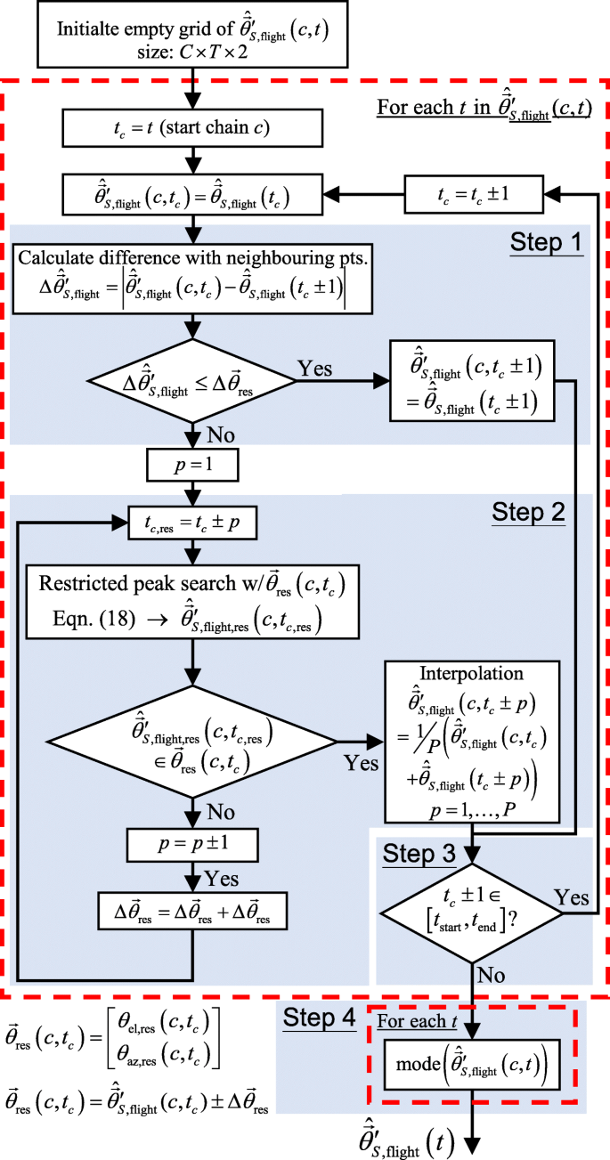

  

  Flowchart of the angular spectral range restricted peak search and link algorithm. The steps highlighted correspond to the steps described in Section 3.3

• 2. Perform restricted peak search using (18) with the SNR response ψflight′(t,τ) (see Fig. 2) and $\vec {\theta }_{\text {res}}(c,t_{c})$ (see Fig. 4) around time frames giving unexpected locations (i.e. exceeding the nominal degree of separation $\Delta \vec {\theta }_{\text {res}}$), and obtaining the correct locations.

• 3. The above steps are repeated until valid locations can no longer be found, or if the start/end of the localisation path has been reached (i.e. t_c±1∉[t_start,t_end]). This forms a “chain” of locations, or a local path (denoted as the cth chain in Fig. 4), to later to be compared against when forming the final global path of locations.

• 4. After obtaining all C chains of local paths, a final path of locations ${\hat {\vec {\theta }}'_{S,\text {flight}}(t)}$ is formed by finding locations that appear most frequently amongst the C chains at the given time frame. Ideally, this would improve the consistency and smoothness compared to the original ${\hat {\vec {\theta }}_{S,\text {flight}}(t)}$.

Finally, the T_flight time frames in ${\hat {\vec {\theta }}_{S,\text {flight}}(t)}$ are aggregated together to obtain ${\hat {\vec {\theta }}''_{S,\text {flight}}(t_{\text {flight}})}$ (see Fig. 2). Details of this process are discussed later in Section 4.1.

The selection of the search range parameter $\Delta \hat {\vec {\theta }}_{\text {res}}$ is heuristically tuned based on whether the estimated path of locations was the most sensible overall (i.e. no aggressive jumps or unnatural changes in direction).

To enable online-processing capabilities to the RPSL post-processing algorithm, this process is carried out in batches of frames of ${\hat {\vec {\theta }}_{S,\text {flight}}(t)}$ that corresponds to 2 second blocks of audio, with the exception of the last batch, which would depend on the number of frames remaining. Such an approach is not uncommon, where online-processing is done via blocks of time frames, rather than individual frames alone [43].

Restricting the angular range for peak search reduces the risk of picking up disturbances with SNR angular spectral response more prominent than that of the target sound source (since they are excluded from the restricted search range). However, this assumes the original localisation path ${\hat {\vec {\theta }}_{S,\text {flight}}(t)}$ is correct in a reasonable portion of the time frames. Conceptually, the method presented here is somewhat similar to the two-step flight path approach from Team Idea!_SSU [1].

Measures are also developed if a particular local path fails to find a peak with high enough SNR response to link towards. For example, the algorithm skips time frames (and proceeds to the next) where the restricted peak search fails to obtain a valid location until one with a valid location is found. Following this, the skipped locations in-between the two valid time frames are obtained via interpolation. Figure 5 shows an example of the improvement in localisation path with each stage (SNR response scaling and RPSL post-processing) of the proposed algorithm applied.

Fig. 5

Example of localisation performance with SNR response scaling (Section 3.2) and RPSL post-processing (Section 3.3) applied. (SPCup flying UAV broadband sound source (task 2) case 11 [1])

4 Experiments

As a team participating in the SPCup, the performance of the proposed method is evaluated against the competition dataset provided by the organiser of the SPCup [1]. Therefore, the proposed algorithm is tuned towards the UAV and microphone array system to develop the dataset. This section presents the details of the experimental setup of the given dataset, including the description of the UAV system, and various constraints found in the dataset. This is followed by an overview of the experimental parameters and additional information used for the proposed method, such as details of the training dataset for the UAV rotor noise PSD estimation process.

4.1 Experimental setup

The proposed method is evaluated using the DREGON database from [44], which makes use of the UAV system shown in Fig. 6. Details of the microphone array and rotor positions are shown in Fig. 7. The UAV is from MicroKopter Ⓡ, utilising the 8 Sounds USB and Many Ears audio processing framework [45]. The UAV system utilises an array of 8 omnidirectional electret condenser microphones, located directly below the centre of the UAV, as shown in Fig. 7. All positions shown in Fig. 7 are in reference to the microphone array’s baricenter.

Fig. 6

Audio recording UAV overview. Image provided by SPCup syllabus [1]

Fig. 7

Microphone array (0–7) and rotor (A–D) geometry overview. Figure provided by SPCup syllabus [1]

Table 1 shows the specifications of the evaluation dataset used for this study. As mentioned in Sections 2 and 3, the proposed method in this study is evaluated against the three tasks. Task 1 contains 300 individual cases; each consists of a ∼3-s microphone array recording for estimating a single location of the target sound source. On the other hand, tasks 2 and 3 consist of 20 cases with broadband sound source and 16 cases with speech sound source used as the target sound source. Each case in tasks 2 and 3 consists of 15 location points to be estimated in 0.25-s intervals along the duration of the 4-s microphone array recording. Therefore, the time frames from the STFT of the recordings are grouped into sections of 6 frames centering around each time-stamp (i.e. t_flight=[0.25s,0.5s,...,3.75s]), with aggregation performed on each of these groups of time frames. Further information regarding the evaluation dataset can be found in Table 1.

4.2 Noise PSD informed SNR response scaling: experimental parameters

To obtain the training and validation dataset required for the DAE from the SNR response scaling algorithm, labelled data containing rotor noise with and without the target source signal is required. Given the dataset is constrained to what was available in the DREGON database, data augmentation had to be performed in order to obtain a sufficient amount of data for training and validation. Initially, individual rotor recordings from the development dataset were used to provide the rotor noise data. However, due to the limited speed range coverage, extracts of rotor noise-only sections from the microphone recordings in the competition dataset were also used as part of the training process. This is achieved by manually editing out sections of the competition audio recordings containing traces of target sound source signals. The rotor noises are then mixed with a corpus of speech recordings to form the input observations, as part of the data augmentation process. For the corpus, the REpeated HArvard Sentence Prompts (REHASP) corpus [46] was used. The sentences were randomly selected with a balanced mixture of male and female speech. Since the individual cases contained in the competition dataset are normalised with respect to its signal amplitude, the rotor noise present in each case would have varying loudness depending on the input SNR. Therefore, one cannot simply train a mapping function by assuming rotor noise is consistent in power, meaning that the training dataset would contain repetitions of the rotor noise audio extracts with different amplitude scaling to compensate for this variation. For broadband sound source, since its acoustical characteristics are unknown, the only obtainable labels were from the development dataset. Thus, these recordings are mixed with the collected UAV rotor noise dataset and included for training.

Table 2 outlines the dataset specifications. To provide generalisation towards the DAE with the available data, the entire training dataset described in Table 2 is used to train a single DAE for each microphone. Given the lack of unique UAV rotor noise data, only 4% of the data from the training dataset described in Table 2 is used to obtain the validation dataset, to preserve as many training data as possible. The observations in the dataset are randomly shuffled prior to the split. For testing, the competition dataset described in Table 1 was used, giving a total of 45,338 observations.

It should be noted that the data constraint workaround described in this study was driven by the limited time and resources in the time of the competition. Ideally, rotor noise recordings would be obtained via independent noise recordings by using the exact UAV system per described in the SPCup syllabus [1], for which a DAE with much higher performance is expected.

4.3 Evaluation metric

The performance of the proposed method is evaluated against the baseline method [27], with GCC-PHAT, GCC-NONLIN, MVDR, DS, and DNM as the localisation techniques (as provided by the SPCup), using both sum and max aggregation (i.e. (13)–(16)). This results in 10 baseline methods to compare against the proposed method. For tasks 2 and 3, due to the proposed method containing two distinct components (SNR response scaling and RPSL post-processing), results with both components applied, as well as those with only one of the components applied, are presented for comparison.

Since the true locations for each test case are unique regardless of the chosen task, instead of directly comparing the estimated locations against the ground truth, the error between the estimated locations and the true locations is calculated and used as the evaluation metric. For the 3D problem presented in this study, the accuracy of the localisation performance is measured by comparing the haversine distance error D [47] (for which will be referred as distance error) between the estimated location $\hat {\vec {\theta }}_{S}$ and the true location $\vec {\theta }_{S}$, assuming a unit sphere (i.e. r=1, such that 0≤D≤π). This is obtained as follows:

$$\begin{array}{*{20}l} \gamma &={{\sin }^{2}}\left(\frac{{{{\hat{\theta }}}_{S,\text{el}}}-{{\theta }_{S,\text{el}}}}{2} \right)\\ &+\cos \left({{{\hat{\theta }}}_{S,\text{el}}} \right)\cos \left({{\theta }_{S,\text{el}}} \right){{\sin }^{2}}\left(\frac{{{{\hat{\theta }}}_{S,\text{az}}}-{{\theta }_{S,\text{az}}}}{2} \right), \end{array} $$

(20)

$$\begin{array}{*{20}l} D=2r{{\sin }^{-1}}\sqrt{\gamma }. \end{array} $$

(21)

Using the haversine distance error measure instead of directly comparing the difference between $\hat {\vec {\theta }}_{S}$ and $\vec {\theta }_{S}$ alleviates the varying sensitivity of ${{{\hat {\theta }}}_{S,\text {az}}}$ to the same amount of error at different ${{{\hat {\theta }}}_{S,\text {el}}}$ (e.g. same amount of angular error in ${{{\hat {\theta }}}_{S,\text {el}}}$ results in significantly different position errors between ${{{\hat {\theta }}}_{S,\text {az}}} = 0$ deg, and ${{{\hat {\theta }}}_{S,\text {az}}} = \pm 90$ deg).

After obtaining the distance error D, its mean, root mean square error (RMSE), maximum, minimum, and quartile measures are compared between the methods. Statistical analysis using the paired sample t test was conducted to evaluate and verify the difference of mean and median errors between the proposed method and each baseline method, respectively. To avoid erroneous inferences caused by multiple comparison, Bonferroni’s correction was applied [48], i.e. for each test, the null hypothesis was rejected by p<0.005 (=0.05/10, given the performance is evaluated against the 10 baseline methods), using the best-performing combination from the proposed method as the benchmark for comparison.

5 Results and discussion

This section presents the experimental results for evaluating the performance of the proposed method against the baseline method as outlined in Section 4.3.

5.1 Task 1: Hovering UAV scenario

Figure 8 shows the distance errors of different localisation methods from task 1, with details of the statistical test results shown in Table 3. As shown, with all baseline techniques using max aggregation, the addition of SNR response scaling delivered improvements with respect to its unscaled baseline. In particular, the MVDR method with max aggregation and SNR response scaling is the best-performing combination. The method outperformed the baseline methods by delivering the lowest mean, maximum, and RMSE distance error measures. Results of the paired sample t test also indicate that the difference of the mean distance error being significantly different against the baseline methods, except GCC-NONLIN using max aggregation. The most apparent improvement is the significant reduction in outlier predictions, which can be seen in Fig. 8, as well as the reduction in the maximum and 0.75 quartile distance errors. This shows that SNR response scaling cleans up the rotor noise effects well, making the SNR response of the target sound source more apparent. Figure 9a, b shows an example of the SNR angular spectral response improvements brought upon using SNR response scaling. Here, influences from the UAV rotor noise are greatly reduced, revealing the peak response of the target sound source. As a result, it brought the estimated location closer to the ground truth. There are still a few cases (cases #59, 61, 70, 159, 160, 178, and 229 in the dataset [1]), which have very low input SNRs, and all methods evaluated (including the proposed method) are not able to give an accurate estimate. Nonetheless, the proposed method has shown a significant improvement in localising accuracy.

Fig. 8

Hovering UAV (task 1)—haversine distance error distribution. Red line indicates the median, upper and lower edges of the blue box indicate the 75% and 25% quartiles, upper and lower black bars indicate the maximum and minimum, and upper and lower corners of the trapezoidal indicate the 95% upper and lower confidence limits

Fig. 9

SNR angular spectral response (dB) from SPCup hovering UAV (task 1) case 297 a w/o SNR response scaling and b w/ SNR response scaling, using MVDR with max aggregation. Circle (∘) and cross (×) in the diagram represent the ground truth and the algorithm’s estimated peak response location, respectively

Table 3 Haversine distance error performance comparison (task 1—hovering UAV)

Apart from GCC-NONLIN, DNM method with max aggregation and SNR response scaling also delivered comparable results. The method delivered lower median and quartile distance error measures, with t test results showing that it is not significantly different to that of the MVDR method using max aggregation and SNR response scaling. However, due to the lower mean and RMSE distance errors, the MVDR method is considered the best-performing combination.

Since the SNR response scaling approach is essentially a T-F mask for filtering out effects of the UAV rotor noise, we compare its performance against other state-of-the-art T-F masks specialised for noisy and reverberant environments, using the study from [28] and [30]. Like SNR response scaling, the T-F mask from [28] is applied to the baseline method. However, given the method is designed for GCC-PHAT, results were only generated under this localisation method. As shown in Fig. 8 and Table 3, the T-F mask from [28] improved the localisation performance overall, reducing the distance error measures with respect to its corresponding baseline. Under the same GCC-PHAT localisation technique, the proposed SNR response scaling method overall outperformed [28] slightly, delivering lower mean, quartile, and RMSE distance error measures. However, with max aggregation, the performance improvement is slight, as suggested by the t test. The T-F mask proposed by [30] is utilised via source enhancement using the minimum mean square error (MMSE) log-spectral amplitude estimator from [49] prior to source localisation using [27]. Contrary to the T-F mask from [28] and the proposed method, the T-F mask from [30] showed mixed performance. While there was general improvement in results with max aggregation, the T-F mask performed worse than the baseline with sum aggregation, with the exception of DS, where both aggregation methods improved over the baseline. Since the T-F mask from [30] assumes continuity in the noise signals, which is a valid assumption, it could have been affected by the vast amount of wind/flow noise generated by the UAV rotors. With the nature of such noise being stochastic, the resultant enhanced signal could have introduced potential distortions. As such, the proposed SNR response scaling method overall outperformed [30] by a visible margin. This indicates that while a diffuse noise-based T-F mask is able to remove some aspects of the noise, a dedicated noise mask designed for UAV rotor noise would still be the desired option.

5.2 Task 2: Flying UAV scenario, broadband sound source

Figure 10 shows the localisation results for task 2, with details of the statistical test results shown in Table 4. Due to the lack of relevant UAV rotor noise data in the flying UAV cases for effective DAE training, the baseline method outperformed the SNR response scaled method under all localisation techniques. Observing the SNR response angular spectrum of the baseline and SNR response scaled method (see Fig. 11a, b), although SNR response scaling reduced noise surrounding the target source location, it came with a peak response for the target source less sharp than the baseline method, as shown in Fig. 11b. This could lead to increased variation in the location path estimations and thus decreasing overall accuracy. It is believed this is caused by the limited amount of available data from the DREGON dataset [44] for training the DAE: a limitation at the point of competition.

Fig. 10

Flying UAV—broadband sound source (task 2) haversine distance error distribution. Red line indicates the median, upper and lower edges of the blue box indicate the 75% and 25% quartiles, upper and lower black bars indicate the maximum and minimum, and upper and lower corners of the trapezoidal indicate the 95% upper and lower confidence limits

Fig. 11

SNR angular spectral response (dB) from SPCup flying UAV broadband sound source (task 2) case 11 a w/o SNR response scaling and b w/ SNR response scaling, using GCC-NONLIN with max aggregation. Cross (×) in the diagram represents the algorithm’s estimated peak response location

Table 4 Haversine distance error performance comparison (task 2—flying UAV, broadband sound source)

In contrast, the proposed method with only the RPSL post-processing algorithm applied outperformed the baseline with most of the localisation techniques, showing improvement in distance error measures, except being GCC-PHAT and GCC-NONLIN with max aggregation, where performance is similar. For this task, GCC-PHAT using sum aggregation is the best-performing combination, as evident in Table 4. In particular, the number of outlier cases significantly reduced, as evident in Fig. 10. This is also evident with localisation techniques other than GCC-PHAT. Since the primary function of GCC-PHAT (and GCC-NONLIN, another well-performing option) involves calculating the cross-correlation between pairs of microphone signals at different TDOAs, it is generally not influenced by spatial aliasing between the microphones and thus, under a certain input SNR, delivers consistent performance. However, as expected from the drawbacks from SNR response scaling, results with both SNR response scaling and RPSL post-processing algorithm applied are not the best-performing combinations. While the combinations reduced mean distance error overall, other metrics such as median and quartile measures delivered mixed results, compared to the baseline method.

An observation that should be noted is the exceptional performance from the baseline method using GCC-NONLIN with sum aggregation. While it is not the best-performing combination under mean and median distance errors, it delivered the lowest RMSE and maximum distance errors. From observing Fig. 10 and Table 4, it is apparent that GCC-NONLIN with sum aggregation is the only combination where there are no significant outliers, while the combination with RPSL post-processing has a single outlier. This could be the leading cause of this result. However, it should be noted that the RPSL post-processed variant presented lower distance error measures in the remaining categories, and thus, the benefits of RPSL should not be overlooked.

From observing the actual location estimates in Fig. 12, while the estimated location path has shown a slightly closer correlation with the ground truth, the RPSL post-processing method seems to have reduced some unstable variations along the location path. Therefore, in some respect, the RPSL algorithm seems to achieve a regularisation effect for the estimation of the path of locations, while bringing the overall location estimates closer to the ground truth. Another one of such example is shown in Fig. 13, the RPSL post-processing algorithm is able to limit the amount of fluctuation in location estimates relative to the baseline method, giving a more stable path.

Fig. 12

Example of localisation path estimated for flying UAV broadband sound source (task 2) case 14 [1], using the baseline and proposed method (RPSL only)

Fig. 13

Example of localisation path estimated for flying UAV broadband sound source (task 2) case 18 [1], using the baseline and proposed method (RPSL only)

Comparing the performance of GCC-PHAT using the proposed method against the T-F mask from [28] showed that both methods could not outperform the baseline. While SNR response scaling alone outperformed [28], when paired with the RPSL post-processing algorithm, [28] outperformed SNR response scaling. In fact, GCC-PHAT using sum aggregation with the T-F mask from [28] and RPSL post-processing is almost arguably the best-performing combination, delivering lowest mean and 0.25 quartile distance error measures, as shown in Table 4. However, due to the same combination without T-F masking giving near-identical performance, except median distance error, for which showed visibly better improvements, was considered the best-performing combination. Perhaps due to the T-F mask not being a data-driven solution, it is more stable against unfamiliar scenarios. Given that the T-F mask is primarily designed for speech signals, with the target source being broadband noise, could be the cause of the lack in performance. The T-F mask from [30] delivered the worst results compared to the other presented methods. Using the best-performing localisation technique (GCC-PHAT) showed that it was unable to outperform both [28] and the proposed method, with or without RPSL post-processing. This is likely driven by the broadband target source, where its diffuse characteristics rendered it difficult to distinguish the time-continuity in the UAV rotor noise from the target sound mixed signal. Overall, SNR response scaling and the T-F mask from [28] and [30] struggled to deliver noticeable improvements in localisation performance.

5.3 Task 3: Flying UAV scenario, speech sound source

Figure 14 shows the localisation results for task 3, with details of the statistical test results shown in Table 5. Similar to the results in task 2, the proposed method using only RPSL post-processing outperformed most baseline methods, delivering lower overall distance error measures under all aspects (mean, median, etc.). Furthermore, the proposed method with both SNR response scaling and RPSL post-processing using many of the localisation techniques also outperformed most baseline methods. In this task, the DS localisation technique with max aggregation and RPSL post-processing is the best-performing combination, delivering the lowest overall mean, median, and quartile distance error measures, with t test results indicating the improvement is distinct.

Fig. 14

Flying UAV—speech sound source (task 3) haversine distance error distribution. Red line indicates the median, upper and lower edges of the blue box indicate the 75% and 25% quartiles, upper and lower black bars indicate the maximum and minimum, and upper and lower corners of the trapezoidal indicate the 95% upper and lower confidence limits

Table 5 Haversine distance error performance comparison (task 3—flying UAV, speech sound source)

One aspect to note is that the many of the localisation techniques using both SNR response scaling and RPSL post-processing delivered lower mean, median, 0.75 quartile, and RMSE measured compared to the same setup without SNR response scaling, as shown in Fig. 14 and Table 5. The only exceptions are MVDR with sum aggregation, DS with max aggregation, and DNM with max aggregation. This indicates that while SNR response scaling lowered the sensitivity in estimating peak response locations more accurately, its ability to reduce unwanted noise is still apparent. Furthermore, under the proposed method with only SNR response scaling, except MVDR with sum aggregation, showed a reduction in maximum distance errors relative to the baseline method. Given that SNR response scaling also improved the performance of MVDR with max aggregation for task 1 suggest that SNR response scaling is still able to deliver some benefits over the baseline method when paired with the RPSL post-processing algorithm. Another potential aspect could be driven by the temporally sparse nature of speech sources. This allows the distinguishing between target and UAV noise sources to be easier than, for example, broadband sources, which is much more continuous and diffuse. However, despite these indications of improvement, further tuning and proper DAE training are still required to bring out the true performance gains of SNR response scaling.

Despite significant improvements in the overall distance error reduction, the accuracy of the predictions for most cases is not yet satisfactory for robust localisation path estimation. This is suspected to be caused by the non-stationary nature of speech (i.e. not all time frames contained the target sound source), which may be an issue with methods based on using the SNR response in angular spectra, according to the previous study [27]. Therefore, the fact that localisation can only be carried out in a limited number of time frames would have caused the proposed method to degrade significantly in performance when the source signal was speech. In addition, the input SNRs in task 3 seem to be much lower than that of other tasks in the DREGON database. This elevates the challenge in estimating the peak response of the target audio source.

Figures 15 and 16 demonstrate two of the more successful path estimates using the proposed method with only RPSL post-processing applied, compared against the baseline method (cases 2 and 3 [1]), using DS with max aggregation. As shown with the baseline method, the low input SNR coupled with speech source being temporally sparser than UAV rotor noise, there are major fluctuations in location estimations. On the other hand, the proposed method with only RPSL post-processing applied is able to estimate some of the locations along the path successfully. As some of the location estimates from the baseline method are correctly estimated, the RPSL post-processing algorithm is able to utilise these data points and perform restricted peak search (see Section 3.3), limiting influences coming from the UAV rotors and reverberation effects, and thereby give a much more accurate path estimate.

Fig. 15

Example of localisation path estimated for flying UAV speech sound source (task 3) case 2 [1], using the baseline and proposed method (RPSL only)

Fig. 16

Example of localisation path estimated for flying UAV speech sound source (task 3) case 3 [1], using the baseline and proposed method (RPSL only)

Figure 17 shows an unsuccessful example of localisation path estimation (case 10 [1]). Here, while there were a few correct estimates of $\hat {\vec {\theta }}_{S,\text {flight}}(t)$ using the baseline method, most are significantly different to that of the ground truth. Therefore, there was a limited basis for the RPSL post-processing algorithm to perform restricted peak search effectively. Therefore, while the variation in localisation path estimate is much less chaotic compared to the baseline method, the overall path is incorrect. A potential method to resolve this deficiency would be to generate an initial $\hat {\vec {\theta }}_{S,\text {flight}}(t)$ that takes in multiple peaks, such as the second and third largest peaks (instead of the single maximum peak), to create a wider grid of location points to perform local path search. Since it is unlikely that the UAV flight path would change in a severely rapid manner, having a larger number of potential local path estimates may grant a higher possibility in successful linking of the correct local paths together. However, exploring the problem further remains as future work.

Fig. 17

Example of localisation path estimated for flying UAV speech sound source (task 3) case 10 [1], using the baseline and proposed method (RPSL only)

Like with task 2, we compare the performance between GCC-PHAT with the proposed method against the T-F mask from [28], and the best-performing localisation technique using the T-F mask from [30] (DS). Again, as shown Fig. 14 and Table 5, both T-F masks and SNR response scaling could not outperform the baseline. Different to that from task 2, while SNR response scaling with max aggregation alone outperformed both [28], this was not the case with sum aggregation. However, when paired with the RPSL post-processing algorithm, SNR response scaling with max aggregation outperformed [28], with sum aggregation showing similar performance. On the other hand, comparing RPSL paired SNR response scaling against the pairing with [30] using DS showed similar performance. Although [30] was able to deliver slightly better performance figures with max aggregation (while SNR response scaling slightly outperformed [30] with sum aggregation), the p value from the paired sample t test indicates that this performance difference is not definitive. Therefore, the performance advantages delivered by SNR response scaling should not be overlooked. In addition, both T-F masks and SNR response scaling with RPSL post-processing outperformed RPSL post-processing alone. This could be driven by the target sound source being speech, where temporal sparsity can be expected, and some aspects of the UAV noise can be distinguished more successfully from the target source.

It should be noted that for both tasks 2 and 3, SNR response scaling suffered significantly from the lack of available training data. As mentioned in Section 4.1, given access to the UAV system for noise recordings, it is expected that noise removal performance would significantly increase with sufficient data available for proper DAE training, thereby improving localisation performance for both target source types. However, this remains a future investigation.

6 Conclusion

A method based on the multi-source TDOA estimation in reverberant audio using angular spectra, to perform sound localisation for a UAV-embedded audio recording system, is proposed. The study proposes extensions to improve localisation accuracy of the baseline method. The extensions include a means of reducing the UAV rotor noise effect via a weighting envelope based on the UAV rotor noise PSD. In addition, the proposed method also introduces an angular spectral range RPSL post-processing algorithm to improve localisation accuracies for the flying (moving) UAV scenario.

Experimental results using the dataset provided by the SPCup show that with proper DAE training, SNR response scaling improves SNR angular spectral response, resulting in a reduction in localisation error. The RPSL post-processing algorithm also displayed improvement in performance consistency even under low input SNR conditions when the source is a non-stationary signal, and the UAV is in motion. Future work includes accessing the UAV system for proper UAV rotor noise data collection, to properly investigate the SNR response scaling’s ability to reduce UAV rotor noise effects under flying UAV scenarios. More challenging scenarios to investigate include rapid movement of the UAV or inclusion of spatially coherent interfering sound sources N_n.

References

A. Deleforge, D. Di Carlo, M. Strauss, R. Serizel, L. Marcenaro, Audio-based search and rescue with a drone: highlights from the IEEE signal processing cup 2019 student competition. IEEE Signal Proc. Mag., 138–144 (2019).
R. Verrier, Drones Are Providing Film and TV Viewers a New Perspective on the Action (Los Angeles Times, 2017). http://www.latimes.com/entertainment/envelope/cotown/la-et-ct-drones-hollywood-20151008-story.html.
M. Margaritoff, An English Lifeboat Crew Is Testing Drones for Search and Rescue (The Drive, 2017). http://www.thedrive.com/aerial/14528/an-english-lifeboat-crew-is-testing-drones-for-search-and-rescue.
A. Charlton, Police Drone to Fly Over New Year’s Eve Celebrations in Times Square (Salon, 2018). https://www.salon.com/2018/12/31/police-drone-to-fly-over-new-years-eve-celebrations-in-times-square_partner.
S. McCarthy, Chinese Police Use Drone to Rescue Man Lost in XinJiang Desert (South China Morning Post, 2018). https://www.scmp.com/news/china/society/article/2168091/chinese-police-use-drone-rescue-man-lost-xinjiang-desert.
A. Lusher, Teenage Rape Victim Found by Police Drone with Thermal Imaging Camera (The Independent, 2018). https://www.independent.co.uk/news/uk/crime/police-drone-thermal-rape-victim-teenager-boston-lincolnshire-surveillance-technology-crime-fighting-a8572656.html.
M. Ablon, Crews: Both Climbers from Looking Glass Rock Rescued, One Taken to Hospital After Nearly 150-Foot Fall (FOX Carolina, 2019). https://www.foxcarolina.com/news/rescuers-searching-for-rock-climbers-at-looking-glass-rock/article_40faa27c-273e-11e9-8d7f-9f80965783a8.html.
Y. Bando, H. Saruwatari, N. Ono, S. Makino, K. Itoyama, D. Kitamura, M. Ishimura, M. Takakusaki, N. Mae, K. Yamaoka, et al, Low latency and high quality two-stage human-voice-enhancement system for a hose-shaped rescue robot. J. Robot. Mechatron.29(1), 198–212 (2017).
Y. Hioka, M. Kingan, G. Schmid, R. McKay, K. A. Stol, Design of an unmanned aerial vehicle mounted system for quiet audio recording. Appl. Acoust.155:, 423–427 (2019).
B. Yen, Y. Hioka, B. Mace, in 2018 16th International Workshop on Acoustic Signal Enhancement (IWAENC). Improving power spectral density estimation of unmanned aerial vehicle rotor noise by learning from non-acoustic information, (2018), pp. 545–549. https://ieeexplore.ieee.org/document/8521324. Accessed 19 Dec 2019.
L. Wang, A. Cavallaro, in 2016 13th IEEE International Conference on Advanced Video and Signal Based Surveillance (AVSS). Ear in the sky: ego-noise reduction for auditory micro aerial vehicles (IEEE, 2016), pp. 152–158. https://ieeexplore.ieee.org/document/7738063. Accessed 19 Dec 2019.
L. Wang, A. Cavallaro, Microphone-array ego-noise reduction algorithms for auditory micro aerial vehicles. IEEE Sensors J.17(8), 2447–2455 (2017).
M. Brandstein, D. Ward, Microphone Arrays: Signal Processing Techniques and Applications, Digital Signal Processing (Springer, 2001). http://link.springer.com/10.1007/978-3-662-04619-7. Accessed 26 June 2017.
P. Marmaroli, X. Falourd, H. Lissek, in Acoustics 2012, ed. by S. F. d’Acoustique. A UAV motor denoising technique to improve localization of surrounding noisy aircrafts: proof of concept for anti-collision systems (Nantes, 2012). https://hal.archives-ouvertes.fr/hal-00811003/document.
K. Furukawa, K. Okutani, K. Nagira, T. Otsuka, K. Itoyama, K. Nakadai, H. G. Okuno, in 2013 IEEE/RSJ International Conference on Intelligent Robots and Systems (IROS). Noise correlation matrix estimation for improving sound source localization by multirotor UAV, (2013), pp. 3943–3948. https://ieeexplore.ieee.org/document/6696920.
K. Washizaki, M. Wakabayashi, M. Kumon, in 2016 IEEE/RSJ International Conference on Intelligent Robots and Systems (IROS). Position estimation of sound source on ground by multirotor helicopter with microphone array (IEEEDaejeon, 2016), pp. 1980–1985. http://ieeexplore.ieee.org/abstract/document/7759312/. Accessed 29 June 2017.
L. Wang, A. Cavallaro, Acoustic sensing from a multi-rotor drone. IEEE Sensors J.18(11), 4570–4582 (2018).
K. Okutani, T. Yoshida, K. Nakamura, K. Nakadai, in Intelligent Robots and Systems (IROS), 2012 IEEE/RSJ International Conference on. Outdoor auditory scene analysis using a moving microphone array embedded in a quadrocopter, (2012), pp. 3288–3293. https://ieeexplore.ieee.org/abstract/document/6385994. Accessed 19 Dec 2019.
T. Ohata, K. Nakamura, T. Mizumoto, T. Taiki, K. Nakadai, in 2014 IEEE/RSJ International Conference on Intelligent Robots and Systems. Improvement in outdoor sound source detection using a quadrotor-embedded microphone array (IEEE, 2014), pp. 1902–1907. https://ieeexplore.ieee.org/document/6942813. Accessed 19 Dec 2019.
K. Nakadai, M. Kumon, H. G. Okuno, K. Hoshiba, M. Wakabayashi, K. Washizaki, T. Ishiki, D. Gabriel, Y. Bando, T. Morito, R. Kojima, O. Sugiyama, in 2017 IEEE/RSJ International Conference on Intelligent Robots and Systems (IROS). Development of microphone-array-embedded UAV for search and rescue task, (2017), pp. 5985–5990. https://doi.org/10.1109/IROS.2017.8206494.
M. Basiri, F. Schill, P. U. Lima, D. Floreano, in 2012 IEEE/RSJ International Conference on Intelligent Robots and Systems. Robust acoustic source localization of emergency signals from micro air vehicles, (2012), pp. 4737–4742. https://ieeexplore.ieee.org/document/6385608. Accessed 19 Dec 2019.
M. Basiri, F. Schill, P. Lima, D. Floreano, On-board relative bearing estimation for teams of drones using sound. IEEE Robot. Autom. Lett.1(2), 820–827 (2016).
T. Ishiki, M. Kumon, in 2014 IEEE International Symposium on Safety, Security, and Rescue Robotics (SSRR). A microphone array configuration for an auditory quadrotor helicopter system, (2014), pp. 1–6. https://ieeexplore.ieee.org/document/7017653. Accessed 19 Dec 2019.
T. Ishiki, M. Kumon, in 2015 IEEE/RSJ International Conference on Intelligent Robots and Systems (IROS). Design model of microphone arrays for multirotor helicopters, (2015), pp. 6143–6148. https://ieeexplore.ieee.org/document/7354252. Accessed 19 Dec 2019.
T. Ishiki, K. Washizaki, M. Kumon, Evaluation of microphone array for multirotor helicopters. J. Robot. Mechatron.29(1), 168–176 (2017).
J. Choi, J. Chang, in 2020 International Conference on Electronics, Information, and Communication (ICEIC). Convolutional neural network-based direction-of-arrival estimation using stereo microphones for drone (Barcelona, 2020), pp. 1–5. https://ieeexplore.ieee.org/document/9051364.
C. Blandin, A. Ozerov, E. Vincent, Multi-source TDOA estimation in reverberant audio using angular spectra and clustering. Signal Process.92(8), 1950–1960 (2012). Latent Variable Analysis and Signal Separation.
R. Lee, M. -S. Kang, B. -H. Kim, K. -H. Park, S. Q. Lee, H. -M. Park, Sound source localization based on GCC-PHAT with diffuseness mask in noisy and reverberant environments. IEEE Access. 8:, 7373–7382 (2020).
W. Zhang, Y. Zhou, Y. Qian, in Proc. Interspeech 2019. Robust DOA estimation based on convolutional neural network and time-frequency masking (Graz-Austria, 2019), pp. 2703–2707. https://www.isca-speech.org/archive/Interspeech_2019/pdfs/3158.pdf.
T. Gerkmann, R. C. Hendriks, Unbiased MMSE-based noise power estimation with low complexity and low tracking delay. IEEE Trans. Audio Speech Language Process.20(4), 1383–1393 (2012).
X. Li, S. Leglaive, L. Girin, R. Horaud, Audio-noise power spectral density estimation using long short-term memory. IEEE Signal Process. Lett.26(6), 918–922 (2019).
Z. -W. Tan, A. H. -T. Nguyen, A. W. -H. Khong, in 2019 Proceedings of Asia-Pacific Signal and Information Processing Association (APSIPA). An efficient dilated convolutional neural network for UAV noise reduction at low input SNR, (2019), pp. 1885–1892.
Y. Hioka, M. Kingan, G. Schmid, K. A. Stol, in 2016 IEEE International Workshop on Acoustic Signal Enhancement (IWAENC). Speech enhancement using a microphone array mounted on an unmanned aerial vehicle, (2016), pp. 1–5. http://ieeexplore.ieee.org/abstract/document/7602937/. Accessed 24 June 2017.
C. Knapp, G. Carter, The generalized correlation method for estimation of time delay. IEEE Trans. Acoust. Speech Signal Process.24(4), 320–327 (1976). https://doi.org/10.1109/TASSP.1976.1162830.
I. McCowan, Microphone Arrays: a Tutorial (Queensland University, Australia, 2001).
H. Cox, R. M. Zeskind, M. M. Owen, Robust adaptive beamforming. IEEE Trans. Acoust. Speech Signal Process.35(10), 1365–1376 (1987).
C. Blandin, E. Vincent, A. Ozerov, in 2011 IEEE International Conference on Acoustics, Speech and Signal Processing (ICASSP). Multi-source TDOA estimation using SNR-based angular spectra, (2011), pp. 2616–2619.
B. Loesch, B. Yang, in 9th International Conference on Latent Variable Analysis and Signal Separation (LVA/ICA). Blind source separation based on time-frequency sparseness in the presence of spatial aliasing, (2010), pp. 1–8.
P. Vincent, H. Larochelle, Y. Bengio, P. -A. Manzagol, in Proceedings of the 25th International Conference on Machine Learning. Extracting and composing robust features with denoising autoencoders (ICMLHelsinki, 2008), pp. 1096–1103. https://dl.acm.org/doi/abs/10.1145/1390156.1390294.
P. Welch, The use of fast fourier transform for the estimation of power spectra: a method based on time averaging over short, modified periodograms. IEEE Trans. Audio Electroacoustics. 15(2), 70–73 (1967).
A. L. Maas, A. Y. Hannun, A. Y. Ng, in ICML Workshop on Deep Learning for Audio, Speech and Language Processing. Rectifier nonlinearities improve neural network acoustic models (ICMLAtlanta, 2013). http://robotics.stanford.edu/~amaas/papers/relu_hybrid_icml2013_final.pdf.
D. P. Kingma, J. Ba, in International Conference on Learning Representations (ICLR). Adam: a method for stochastic optimization (ICLRSan Diego, 2015). https://arxiv.org/abs/1412.6980.
Y. Bando, K. Itoyama, M. Konyo, S. Tadokoro, K. Nakadai, K. Yoshii, T. Kawahara, H. G. Okuno, Speech enhancement based on bayesian low-rank and sparse decomposition of multichannel magnitude spectrograms. IEEE/ACM Trans. Audio Speech Lang. Process.26(2), 215–230 (2018).
M. Strauss, P. Mordel, V. Miguet, A. Deleforge, in 2018 IEEE/RSJ International Conference on Intelligent Robots and Systems (IROS). Dregon: dataset and methods for uav-embedded sound source localization (IROSMadrid, 2018), pp. 1–8. https://ieeexplore.ieee.org/abstract/document/8593581/.
F. Grondin, D. Létourneau, F. Ferland, V. Rousseau, F. Michaud, The manyears open framework. Auton. Robot.34(3), 217–232 (2013).
G. E. Henter, T. Merritt, M. Shannon, C. Mayo, S. King, in Fifteenth Annual Conference of the International Speech Communication Association. Measuring the perceptual effects of modelling assumptions in speech synthesis using stimuli constructed from repeated natural speech, (2014).
R. W. Sinnott, Virtues of the haversine. Sky Telesc.68:, 159 (1984).
F. Curtin, P. Schulz, Multiple correlations and Bonferroni’s correction. Biol. Psychiatry. 44(8), 775–777 (1998).
Y. Ephraim, D. Malah, Speech enhancement using a minimum mean-square error log-spectral amplitude estimator. IEEE Trans. Acoust. Speech Signal Process.33(2), 443–445 (1985).
Acknowledgements
We would like to give our thanks to the Acoustics Research Centre, University of Auckland, for supporting this project. We would also like to thank Alec Handyside, James Kennelly, Dylan Leslie, and Weichi Liu for their work and effort as a team in the development of the study’s proposed method for the 2019 IEEE SPCup.
Funding
This study was funded by the Acoustics Research Centre, University of Auckland.
Author information
Authors and Affiliations
Contributions
Benjamin Yen led the University of Auckland student team in the participation of the 2019 IEEE SPCup, including algorithm development, prototyping, and tuning. Benjamin Yen prepared the manuscript. Yusuke Hioka led the initiative of the study and supervised Benjamin Yen. Yusuke Hioka and Benjamin Yen reviewed edited the manuscript. All authors read and approved the manuscript.
Corresponding author
Ethics declarations
Competing interests
The authors declare that they have no competing interests.
Additional information
Publisher’s Note
Springer Nature remains neutral with regard to jurisdictional claims in published maps and institutional affiliations.
This study is based on a contribution to the 2019 IEEE Signal Processing Cup (SPCup): Audio-Based Search and Rescue with a Drone \citedeleforge:hal-02161897.
Rights and permissions
Open Access This article is licensed under a Creative Commons Attribution 4.0 International License, which permits use, sharing, adaptation, distribution and reproduction in any medium or format, as long as you give appropriate credit to the original author(s) and the source, provide a link to the Creative Commons licence, and indicate if changes were made. The images or other third party material in this article are included in the article’s Creative Commons licence, unless indicated otherwise in a credit line to the material. If material is not included in the article’s Creative Commons licence and your intended use is not permitted by statutory regulation or exceeds the permitted use, you will need to obtain permission directly from the copyright holder. To view a copy of this licence, visit http://creativecommons.org/licenses/by/4.0/.
About this article
Cite this article
Yen, B., Hioka, Y. Noise power spectral density scaled SNR response estimation with restricted range search for sound source localisation using unmanned aerial vehicles. J AUDIO SPEECH MUSIC PROC. 2020, 13 (2020). https://doi.org/10.1186/s13636-020-00181-5
Received:
Accepted:
Published:
DOI: https://doi.org/10.1186/s13636-020-00181-5