


1. Introduction
The Taylor–Couette system, a canonical flow geometry, has been bestowed with honorifics such as ‘hydrogen atom of fluid dynamics’ (Tagg Reference Tagg1994) as well as ‘Drosophila’ (van Gils et al. Reference van Gils, Huisman, Grossmann, Sun and Lohse2012). This is with good reason, as it has served as a very simple system to address fundamental problems in physics such as instabilities, nonlinear dynamics, pattern formation, spatio-temporal chaos and turbulence (Grossmann, Lohse & Sun Reference Grossmann, Lohse and Sun2016). Furthermore, this flow apparatus is also of interest to application-oriented research, primarily concerning chemical processing (see table 1 in Zhu & Vigil Reference Zhu and Vigil2001 for numerous examples). This geometry also forms the skeleton of the contemporary rheometer, and is commonly used for measuring dynamic viscosities of fluids (Guazzelli & Pouliquen Reference Guazzelli and Pouliquen2018).
While the initial Taylor–Couette apparatus were dedicated to the determination of fluid dynamic viscosity (Couette Reference Couette1890; Mallock Reference Mallock1896), the now near-century old, seminal contribution of Taylor (Reference Taylor1923) laid the foundation for future work in this field. The work of Taylor (Reference Taylor1923) established the critical conditions necessary for the appearance of secondary flow structures, subsequently known as Taylor vortices (pair of counter-rotating vortices, stacked axially), when the flow is driven by a rotating inner cylinder. The critical conditions are commonly quantified by means of a Reynolds number, or even a Taylor number. Further increase in the rotational velocity of the cylinder leads to additional instabilities, such as the appearance of wavy vortices (Coles Reference Coles1965), modulated wavy vortices (Gorman & Swinney Reference Gorman and Swinney1982; Zhang & Swinney Reference Zhang and Swinney1985), before the onset of chaos (Gollub & Swinney Reference Gollub and Swinney1975; Fenstermacher, Swinney & Gollub Reference Fenstermacher, Swinney and Gollub1979) and turbulence (Koschmieder Reference Koschmieder1979; Lathrop, Fineberg & Swinney Reference Lathrop, Fineberg and Swinney1992; Lewis & Swinney Reference Lewis and Swinney1999). Initial studies primarily involved the usage of Newtonian fluids, and this alone provided a plethora of intriguing flow phenomena, by either varying the flow geometry or the nature of the cylinder rotation (i.e. inclusion of outer cylinder rotation). Consequently, an extensive study of the various flow patterns has resulted in the comprehensive flow regime map compiled by Andereck, Liu & Swinney (Reference Andereck, Liu and Swinney1986). Contemporary single-phase Taylor–Couette flows have been predominantly geared towards understanding high-Reynolds-number turbulence (Grossmann et al. Reference Grossmann, Lohse and Sun2016), where the bulk flow as well as the two boundary layers are turbulent in nature.
In the century since Taylor's seminal work, the studied phenomena within this simple flow geometry have branched significantly. Newer forms of instabilities and flow phenomena have been uncovered by simply changing the fluid within the Taylor–Couette geometry. Along this line, the study of unusual flow patterns in a neutrally buoyant, non-Brownian, particle-laden suspension, arising due to inertial effects, has recently gained traction. This is exemplified in the recent works of Majji, Banerjee & Morris (Reference Majji, Banerjee and Morris2018) and Ramesh, Bharadwaj & Alam (Reference Ramesh, Bharadwaj and Alam2019), where both studies successfully uncover novel flow patterns stemming from the additional presence of solid particles. Majji et al. (Reference Majji, Banerjee and Morris2018) were the first to report the occurrence of non-axisymmetric flow structures (ribbons and spirals) as primary instabilities. An experimental protocol with decreasing inertia in time was preferred over one with increasing, as axial non-homogeneities in the particle distribution were observed for the latter. Ramesh et al. (Reference Ramesh, Bharadwaj and Alam2019) extended on this by also considering an experimental protocol with increasing inertia, which gave rise to the so-called ‘coexisting states’ (presence of axially segregated flow states, such as the combination of wavy and Taylor vortices or Taylor and spiral vortices). More recently, Ramesh & Alam (Reference Ramesh and Alam2020) also reported the existence of interpenetrating spiral vortices in such flows.
Changes in the nature of the suspension was also the theme of one of the pioneering works in the field of non-Brownian particle-laden flows, namely the experiments of Bagnold (Reference Bagnold1954) (later re-examined by Hunt et al. Reference Hunt, Zenit, Campbell and Brennen2002). Torque measurements of neutrally buoyant particle-laden suspensions in a Taylor–Couette geometry driven by a rotating outer cylinder yielded two distinct flow regimes which were characterized on the basis of their respective scaling law behaviours. Thus, besides flow visualization techniques, torque measurements are capable of providing complementary, global information of the flow topology, as also evidenced in several single-phase, turbulent Taylor–Couette flow studies (Wendt Reference Wendt1933; Lathrop et al. Reference Lathrop, Fineberg and Swinney1992; Eckhardt, Grossmann & Lohse Reference Eckhardt, Grossmann and Lohse2007).
The flow visualization studies of Majji et al. (Reference Majji, Banerjee and Morris2018), Ramesh et al. (Reference Ramesh, Bharadwaj and Alam2019) and Ramesh & Alam (Reference Ramesh and Alam2020) restrict their studied range of flow topologies up to the appearance of wavy Taylor vortices. To the best of our knowledge, there are no systematic studies explicitly pursuing the development of flow regimes beyond the appearance of wavy vortices for neutrally buoyant, non-Brownian particle-laden suspensions in a Taylor–Couette geometry driven by inner cylinder rotation. Studying these higher-order transitions can provide insight into the phenomena leading to the transition to turbulence.
To this end, the current study aims to add on to the existing body of work, in an existing Taylor–Couette facility (Ravelet, Delfos & Westerweel Reference Ravelet, Delfos and Westerweel2010), with the manuscript addressing the following issues.
(i) We study the lower-order transitions in our Taylor–Couette geometry (i.e. until the first appearance of wavy vortices), in order to verify whether the current experiments also yield non-axisymmetric flow patterns. Differences from previous studies could be expected since the current experiments are performed under different conditions (discussed later in § 2.8).
(ii) We also pursue flow transitions beyond the appearance of wavy vortices, i.e. higher-order transitions. We investigate whether there is a qualitative change in these transitions as compared to single-phase flows.
(iii) We assimilate the effect of flow inertia and particle loading on the required torque to sustain the flow, into an empirical scaling law.
The above points are addressed experimentally by means of simultaneous flow visualization and torque measurements. The remainder of the manuscript is structured as follows: In § 2 the finer details of the experimental set-up, the measurement procedure as well as experimental uncertainties are described. Hereafter, a global overview of our experimental results is presented in § 3, focusing on flow visualization (§ 3.1) as well as torque measurements (§ 3.2). For the torque measurements, we derive an empirical scaling law relating the measured torque, the driving force and the particle loading. Three detailed flow visualization examples for different particle volume fractions are then used to illustrate the nature of lower- as well as higher-order transitions in §§ 4 and 5, respectively. Among the lower-order transitions, special attention is given to a novel flow state, ‘azimuthally localized wavy vortex flow’ in § 4.5. We summarize our key findings in § 6, while also specifying possible future directions that can be undertaken to consolidate/expand upon our findings.
2. Experimental set-up and measurement procedure
Details of the experimental set-up and the various measurement techniques employed are presented in this section. Readers interested in further details of the experimental set-up and procedures are referred to Anantharaman (Reference Anantharaman2019). The chief components of the set-up are illustrated in figure 1. Note that the torque measurements and the flow visualization recordings were performed simultaneously.
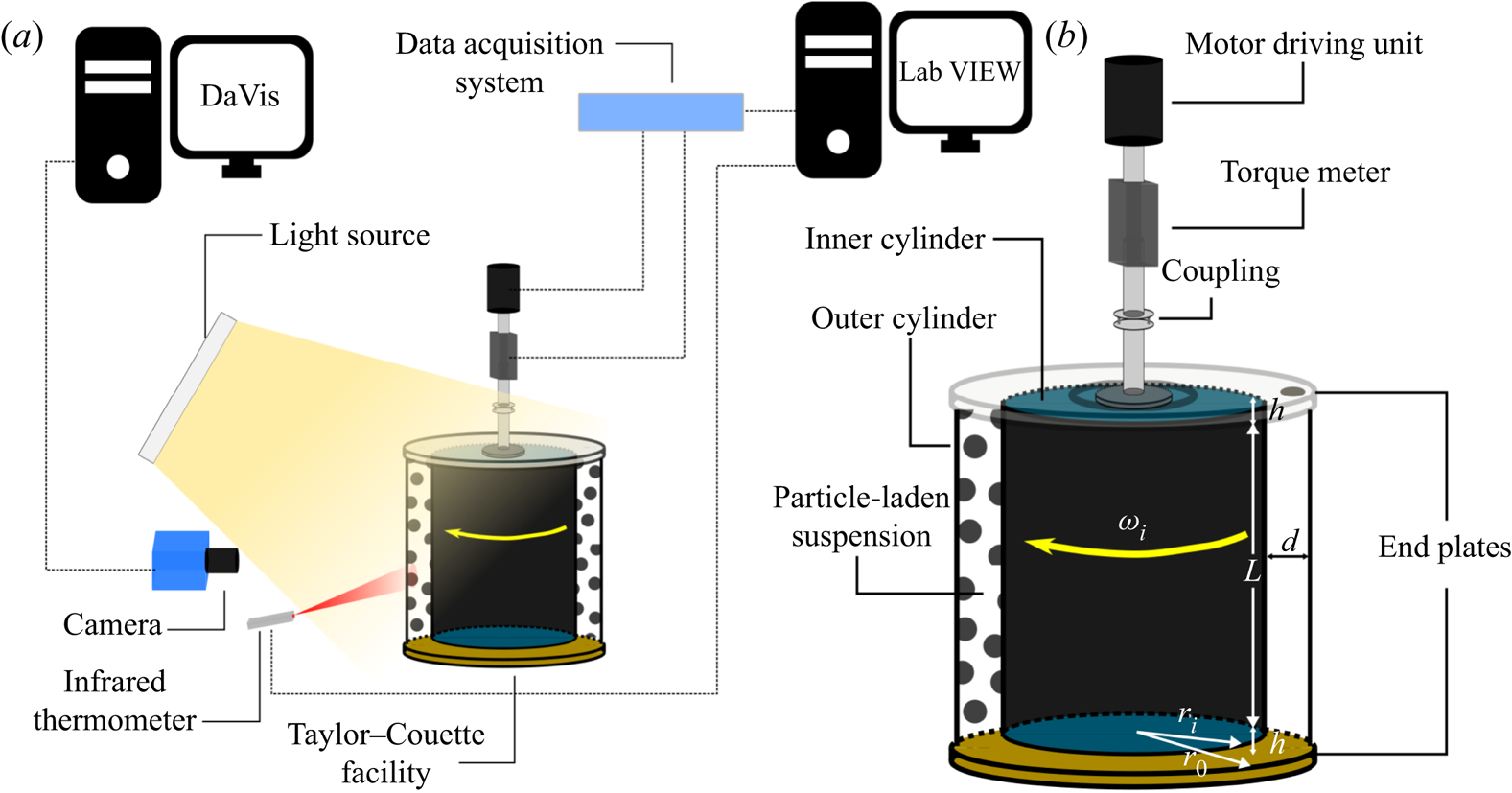
Figure 1. Schematic of the experimental set-up and measurement equipment involved. Objects are not drawn to scale. (a) Experimental set-up and measurement apparatus. (b) A close-up of the Taylor–Couette geometry.
2.1. Geometry of the Taylor–Couette facility
The Taylor–Couette facility used in the current investigation is composed of two vertical, coaxial, concentric and independently rotatable cylinders. The inner cylinder has a radius ( $r_i$) of 11 cm and the outer cylinder has a radius (
 $r_o$) of 12 cm. This leads to the current system having an annular gap width (
 $d = r_o - r_i$) of 1 cm and a radius ratio (
 $\eta = r_i/r_o$) of 0.917. The inner cylinder has a height (
 $L$) of 21.67 cm, while the outer cylinder has a height of 22.21 cm, leading to the formation of two end gaps, each with a height of 2.70 mm. Thus, the present geometry has an aspect ratio (
 $\varGamma = L/d$) of 21.67. The present system may thus be categorized as a narrow gap (
 $1-\eta \ll 1$) and relatively tall (
 $\varGamma \geq 20$). In the current experiments, the outer cylinder is held at rest, while the inner cylinder has a rotational velocity,
  $\omega _i$, which is determined by the desired rotational frequency,
  $f_i = \omega _i/(2{\rm \pi} )$. The inner cylinder velocity
  $U_i = \omega _i r_i$ is the source for the shear and the apparent shear rate can be defined as the ratio between the inner cylinder velocity and the gap width,
  $\dot {\gamma }_{{app}} = U_i/d = (\omega _i r_i)/d$.
With the help of these parameters, several non-dimensional control parameters can be defined. For a working fluid with a density,  $\rho$, and dynamic viscosity,
  $\mu$ (thus, kinematic viscosity
  $\nu = \mu /\rho$), the inner cylinder Reynolds number is defined as
  $Re = (\omega _i r_i)d/\nu = \dot {\gamma }_{{app}} d^2/\nu$. Alternatively, the Taylor number,
  $Ta = K\,Re^2$ may also be used, where the prefactor
  $K = (1+\eta )^6/(64\eta ^4) = 1.0971$ is related to the geometry of the Taylor–Couette facility via the geometric Prandtl number (Eckhardt et al. Reference Eckhardt, Grossmann and Lohse2007).
Surfaces of both the cylinders are made of polymethylmethacrylate (PMMA), facilitating optical access. However, the inner surface of the hollow, inner cylinder (thus, not in contact with the fluid) is painted black to avoid reflections from the structural metal bars present inside the inner cylinder. The inner cylinder is sealed shut by means of PVC discs (which rotate with the inner cylinder), whereas the outer cylinder has end plates made of a PMMA base with a brass ring (bottom) and aluminium (top), both of which would rotate together with the outer cylinder.
2.2. Preparation of the neutrally buoyant suspension
The Taylor–Couette facility was filled with a nearly neutrally buoyant suspension consisting of rigid PMMA particles in an aqueous glycerol solution ( ${\sim }67.6\,\%$ v/v), with a density of
  $1187.7\ \textrm {kg}\,\textrm {m}^{-3}$ and a dynamic viscosity of
  $28.7\ \textrm {mPa}\,\textrm {s}$ at
  $20\, ^{\circ }\textrm {C}$. The continuous phase was prepared by mixing appropriate quantities of demineralized water with an aqueous glycerol solution with a specific gravity of 1.23 (Boom BV, The Netherlands). The two components were mixed together, while stirring and warming the mixture simultaneously, before adding a small quantity of Tween-20 (
 $0.1\,\%$ by volume), a surfactant, which aids in suspending hydrophobic particles. The effect of the surfactant on properties such as density and viscosity was neglected, since it is added in a very small amount.
Rigid PMMA particles (PMMA powder – acrylic, injection moulding grade, Goodfellow USA) were used as the dispersed phase. A sieving procedure was used to narrow the distribution of particle sizes. An inspection of a small sample of particles ( ${\sim }675$) under a microscope, equipped with a Nikon objective
  $M \times 1.0/0.4$ lens, yielded the following information. The majority of the particles are smooth spheres with a few of them possibly having voids within, which are clearly visible as PMMA is optically transparent. The median particle diameter (commonly referred to as
  $d_{p,50}$, but as
  $d_p$ in this manuscript) was found to be
  $599\ \mathrm {\mu }\textrm {m}$. This results in a gap width to particle diameter ratio (
 $d/d_p$) of approximately 16.7.
The sieved particles were then dispersed in the aqueous glycerol mixture by means of a magnetic stirrer. After mixing for a few minutes, the suspension was allowed to rest for approximately 20 min. It was observed that there is a thicker layer of particles creaming to the top as compared to those which sediment to the bottom. These creaming particles could possibly be light because of the presence of internal voids, which are removed before the batch is introduced into the flow.
Suspensions are commonly characterized by an effective suspension viscosity (Guazzelli & Pouliquen Reference Guazzelli and Pouliquen2018). Of the several existing viscosity laws, we utilize fits of the nature proposed first by Eilers (Reference Eilers1941),  $\mu _{{susp}}/\mu = [1+1.25\phi /(1-\phi /\phi _c)]^2$, where
  $\phi _c$ is the volume fraction of particles beyond which the suspensions cease to flow, which is usually lower than the random close packing (
 ${\approx }0.64$). We have chosen a value of
  $\phi _c = 0.614$ (verified with torque measurements as a reasonable choice). The subscript ‘susp’ is henceforth utilized when the effective suspension viscosity is used instead of that of the continuous phase.
2.3. Rotation control and torque measurements
The inner cylinder is driven by a Maxon DC motor, via a shaft and flexible coupling mechanism. The cylinder can be rotated (in both directions) up to a rotational frequency of 10 Hz with an absolute resolution of 0.01 Hz. Furthermore, to verify whether the desired rotational frequency matches the actual rotational frequency of the inner cylinder, a TTL frequency counter returns a pulse every  $36^{\circ }$ rotated by the inner cylinder, i.e. 10 pulses for a complete rotation. The frequency determined by the TTL frequency counter is subsequently used for estimating the apparent shear rates and Reynolds numbers. The input to the motor is controlled by a custom-made LabVIEW program via a data acquisition (DAQ) block (NI PCI-6035E) and a 12-bit DAQ board (NI BNC-2110).
The same data acquisition system is also used to record the torque,  $T$, experienced by the entire inner cylinder, via a torque meter (HBM T20 WN, 2 Nm) attached to the shaft of the inner cylinder. This meter can measure torques up to 2 Nm with an absolute resolution of 0.01 Nm, and is sampled at a frequency of 2 kHz in the current study.
The relative motion between the end plates of the two cylinders may also be likened to a von Kármán swirling flow. This motion would contribute to additional torque, while also spawning vortices due to the so-called Ekman pumping, commonly referred to as end effects. Since the torque measurements also include contributions from the von Kármán flow, the torque is simply halved, in line with previous studies in the same facility (Ravelet et al. Reference Ravelet, Delfos and Westerweel2010). This assumption was later verified by Greidanus et al. (Reference Greidanus, Delfos, Tokgoz and Westerweel2015) to be analytically valid for laminar flows in the current facility. We assume that this is also valid for non-laminar, particle-laden flows. A fragmented inner cylinder design (Lathrop et al. Reference Lathrop, Fineberg and Swinney1992; van Gils et al. Reference van Gils, Bruggert, Lathrop, Sun and Lohse2011) would be needed to eliminate the influence of the ends on torque measurements.
The torque can then be modified into several non-dimensional variants, such as dimensionless torque,  $G = T/(L\rho \nu ^2)$, friction coefficient,
  $c_f = T/({\rm \pi} \rho r_i^2 L U_i^2)$ and the Nusselt number,
  $Nu_{\omega } = T/(2{\rm \pi} L \rho J^{\omega }_{lam})$, where
  $J^{\omega }_{lam} = 2\nu r_i^2 r_o^2 \omega _i/(r_o^2 - r_i^2)$ is the azimuthal flux of the angular velocity between the two cylinders for purely laminar flow. The above three quantities are related to each other (Grossmann et al. Reference Grossmann, Lohse and Sun2016).
2.4. Temperature estimation
The current facility lacks a temperature control system, which would ideally alleviate the negative effect of heating of the fluid by viscous dissipation. As a consequence, the dynamic/kinematic viscosity of the fluid may undergo significant changes. Previous studies in the same facility have sought solutions such as ensuring that the temperature did not vary by more than  $0.5 \, ^{\circ }\textrm {C}$ (Tokgoz et al. Reference Tokgoz, Elsinga, Delfos and Westerweel2012), or by running the system for a few hours prior to the measurements, ensuring a stable temperature thereafter (Gul, Elsinga & Westerweel Reference Gul, Elsinga and Westerweel2018). Such measures were not applicable for the current investigation due to the nature of the experimental protocol and, thus, an ad hoc approach to estimate the varying temperature throughout the experiments is adopted (similar to Greidanus et al. Reference Greidanus, Delfos, Tokgoz and Westerweel2015; Benschop et al. Reference Benschop, Guerin, Brinkmann, Dale, Finnie, Breugem, Clare, Stübing, Price and Reynolds2018).
Before and after each experiment, a PT-100 sensor is inserted into the system through an opening on the top end plate attached to the outer cylinder, to measure the fluid/suspension temperature (under the assumption of isothermal conditions). Since the above intrusive method is not feasible during the experiment, an infrared thermometer (Calex PyroPen) measures the temperature of the outer surface of the outer cylinder at a sampling rate of 1 Hz. The emissivity constant in the proprietary software, CalexSoft, responsible for these measurements, is set as 0.86 (corresponding to the PMMA surface). Combining the above temperature measurements (PT-100 + infrared thermometer), ‘instantaneous’ temperatures of the suspension, and, thus, ‘instantaneous’ Reynolds numbers for the flow, can be estimated. This is extremely handy as the viscosity of an aqueous Glycerol solution is very sensitive to temperature changes ( ${\approx }5\,\% \, ^{\circ }\textrm {C}^{-1}$ at temperatures around
  $20\, ^{\circ }\textrm {C}$ for the current composition of the solution). Typical temperature variations in the current experiments were in the order of
  $5\, ^{\circ }\textrm {C}$, necessitating this ad hoc technique for temperature estimation. The estimated temperatures were then utilized to compute the instantaneous physical properties of the fluid by an open source, freely available Matlab script (based on Cheng Reference Cheng2008; Volk & Kähler Reference Volk and Kähler2018).
2.5. Experimental protocol
In this manuscript we distinguish suspension Reynolds number ( $Re_{{susp}}$) from the Reynolds number (
 $Re$). The former is based on an effective suspension viscosity while the latter only on the viscosity of the continuous liquid phase. We cover a wide range of suspension Reynolds numbers
  $(Re_{{susp}} \sim O(10^1\text {--}10^3))$ for a wide variety of volume fractions
  $(0 \leq \phi \leq 0.40)$. Moreover, it is desired that these large ranges of Reynolds numbers are sampled fine enough to have a clear picture of the transitions between various flow regimes. Recent experiments of Majji et al. (Reference Majji, Banerjee and Morris2018) and Ramesh et al. (Reference Ramesh, Bharadwaj and Alam2019) were performed for a similar range of volume fractions, but for a lower range of Reynolds numbers
  $(Re_{{susp}} \sim O(10^2))$. These two studies utilized slowly accelerating/decelerating ramp protocols, i.e.
  $\textrm {d}\,Re/ \textrm {d}\tau \ll 1$. Here,
  $\tau = t/(d^2/\nu )$ is dimensionless time where the time
  $t$ is normalized by a time scale based on viscous diffusion (
 $d^2/\nu$).
Dutcher & Muller (Reference Dutcher and Muller2009) showed that the critical  $Re$ at which the flow transitions from laminar Couette flow to Taylor vortex flow was a function of the ramp rate, and define a critical ramp rate (ramp rate below which the critical
  $Re$ is in good agreement with linear stability theory) of
  $\textrm {d}Re/\textrm {d}\tau = 0.68$ for their experiments (
 $\eta = 0.912, \varGamma = 60.7$). Moreover, they report a low deviation in the critical Reynolds number with varying ramp rates for higher-order transitions such as wavy vortex flow and modulated wavy vortex flow for
  $0.18 < \textrm {d}Re/\textrm {d}\tau < 2.93$, while also finding no effect of the ramp rate on the onset of turbulent Taylor vortices for
  $\textrm {d}Re/\textrm {d}\tau < 27.2$. In a similar vein, Xiao, Lim & Chew (Reference Xiao, Lim and Chew2002) (
 $\eta = 0.894, \varGamma = 94$) report an absence of dependence of the characteristics of the wavy vortex flow regime for ramp rates
  $\textrm {d}Re/\textrm {d}\tau < 11.2$. Of course, a caveat is that the above statements are valid for single-phase flows and whether the same would be directly applicable for suspensions is unknown.
For the current experiments, following a ramp rate of  $|\textrm {d}Re/\textrm {d}\tau | \ll 1$ would require an unreasonable amount of time to cover the entire span of control parameters (
 $Re, \phi$), and thus a compromise is reached, which ensures a practical approach (similar to Cagney & Balabani Reference Cagney and Balabani2019). The apparent ramp rate is maintained at
  $|\textrm {d}Re/\textrm {d}\tau | < 3$. We define the apparent ramp rate as the ratio between the net differential change in Reynolds number and the net differential change in dimensionless time. These net differential changes are the difference between the values at the start and end of the protocol, making the apparent ramp rate a global measure of our experimental protocol. Of course, it must be noted that if the effective suspension viscosity is taken into account for the
  $Re$ as well as
  $\tau$, i.e.
  $|\textrm {d}Re_{{susp}}/\textrm {d}\tau _{{susp}}|$, the apparent ramp rates will drop sharply with increasing
  $\phi$. For example, for
  $\phi = 0.10$, a reduction with a factor of 1.75 will occur, whereas for
  $\phi = 0.30$, this factor shall be approximately 9. In conclusion, we expect that our choice of ramp rate may affect the accurate determination of precise transition boundaries for dilute suspensions. However, the chosen ramp rate is not expected to affect the flow topologies themselves, which is acceptable for the present study.
Two types of experimental protocols are followed: the Reynolds number of the inner cylinder is slowly raised (reduced, respectively) with time by increasing (decreasing) the apparent shear rate. We change  $\dot {\gamma }_{{app}}$ in steps of
  $3.5\ \textrm {s}^{-1}$ for
  $\dot {\gamma }_{{app}} \leq 69.1\ \textrm {s}^{-1}$ and steps of
  $6.9\ \textrm {s}^{-1}$ for
  $\dot {\gamma }_{{app}} > 69.1\ \textrm {s}^{-1}$. Maximum shear rates of
  $414.7\ \textrm {s}^{-1}$ are achieved for all suspensions with
  $\phi \leq 0.20$. For suspensions with
  $0.25 \leq \phi \leq 0.35$, the maximum shear rate studied is
  $380.1\ \textrm {s}^{-1}$ and
  $276.5\ \textrm {s}^{-1}$ for
  $\phi = 0.40$, in order not to exceed the maximum torque acceptable for the torque meter. In summary, the shear rate is ramped up (down) in a quasi-static manner with non-infinitesimal steps. At each step, the shear rate is held constant for a period of 90 s and between two steps, the flow is accelerated (decelerated) at a rate of
  $3.5\ \textrm {s}^{-2}$ (thus,
  $|\textrm {d}Re/\textrm {d}\tau | \sim 90$ between two steps, which is a local measure of the ramp rate unlike the apparent ramp rate). These protocols are henceforth referred to as ‘ramp-up’ (‘ramp-down’). Please note that these two experiments are done separately, like Ramesh et al. (Reference Ramesh, Bharadwaj and Alam2019). A few experiments were repeated on different days, and sufficient repeatability was observed.
Before the ramp-up experiments, the flow is sheared for a few minutes at a high shear rate, homogenizing the dispersed phase as well as the visualization flakes (see § 2.6) across the system. After allowing the system to be at rest for approximately 20 min, facilitating the decay of residual motions, the experiments are started. For the ramp-down experiments, the flow is accelerated to the highest desired shear rate at a rate of  $3.5\ \textrm {s}^{-2}$ (
 $|\textrm {d}Re/\textrm {d}\tau | \sim 90$, a local measure of the ramp rate unlike the apparent ramp rate) and sheared for five minutes before starting the actual measurements.
A typical example of the realized experimental protocol is illustrated in figure 2 for  $\phi = 0.10$. While the apparent shear rates are in line with expectations (figure 2a), the considerable change in the kinematic viscosity (figure 2b, on occasions up to 20 % variations) manifests itself in nonlinear profiles between the Reynolds number and non-dimensional time (figure 2c). In the ramp-up experiments the viscosity decreases monotonically, as the magnitude of viscous heating only increases with time. In contrast, for the ramp-down experiments, the viscosity profile is often non-monotonic in time. The initial reduction in viscosity is driven by the temperature rise due to viscous heating, while later, the increase in viscosity (thus lowering of temperature) may be attributed to heat loss mechanisms dominating heat generated by viscous dissipation. These profiles also suggest that solely relying on temperature measurements before and after experiments could be misleading for a ramp-down experiment – even though the net change might not be much, the viscosity would have varied quite significantly over the course of the experiment. Ultimately, in the ramp-down experiments the Reynolds numbers profile may also appear non-monotonic (reduction in viscosity dominates reduction in apparent shear rates, initially). The apparent ramp rate,
  $|\textrm {d}Re/\textrm {d}\tau |$, for the ramp-down experiment in this example is
  ${\sim }|(0-3000)/(1000-0)| \sim 3$. If suspension viscosity is considered,
  $|\textrm {d}Re_{{susp}}/\textrm {d}\tau _{{susp}}|$, then the apparent ramp rate becomes
  ${\sim } |(0-2271)/(1321-0)| \sim 1.7$.

Figure 2. Example of the temporal variation of the control parameters for ramp-up and ramp-down protocols ( $\phi = 0.10$). (
 $a$) Apparent shear rate. (
 $b$) Estimated kinematic viscosity of the working fluid/suspension. (
 $c$) The estimated (suspension) Reynolds number. The dash–dotted lines in (
 $c$) are representative of the apparent ramp rate.
2.6. Flow visualization
For the classification of flow regimes, the well-established technique of flow visualization is employed. To this end, a small quantity of Iriodin 100 silver pearl (Merck KGaA, Darmstadt, Germany) is added to the suspension, 0.1 % by mass. The size of these anisotropic flakes is specified by the manufacturers to be between  $10 \text { and }60\ \mathrm {\mu }\textrm {m}$ with a density between 2800 and
  $3000\ \textrm {kg}\,\textrm {m}^{-3}$. Given the low volume fraction of these flakes present, and their relative smaller size (by an order of magnitude, compared to the dispersed phase as well as the geometry), their effect on the flow behaviour is assumed to be negligible. The anisotropic flakes align themselves with the stream surfaces (Savaş Reference Savaş1985) and any reflected light is attributed to the rotational motion of these flakes (Gauthier, Gondret & Rabaud Reference Gauthier, Gondret and Rabaud1998).
The light source illuminating the flakes is an LED panel, which is mounted at an oblique angle, above the flow facility, to minimize specular reflections onto the camera. The light reflected back by the flakes is recorded by a LaVision Imager sCMOS 16-bit camera equipped with a Nikon 35 mm lens ( $f_{\#} = 4$). The pixel pitch of the camera is
  $6.5\ \mathrm {\mu }\textrm {m}$ and images with sizes up to a maximum of
  $2560 \times 2160$ pixels can be captured. This covers a field-of-view of approximately
  $28.1 \times 23.7\ \textrm {cm}^{2}$ in the current experiments, while providing a resolution of
  $0.11\ \textrm {mm}\,\textrm {pixel}^{-1}$ along the axial direction. Images are recorded with an exposure time of
  $1500\ \mathrm {\mu }\textrm {s}$ and a frame rate of 50 Hz. In order to record at a higher frame rate of 100 Hz, the sensitive region of the camera was cropped in one direction to yield images of sizes
  $2560 \times 200$ pixels. The camera is focused onto the outer surface of the outer cylinder by means of a custom-made calibration target. No special measures are implemented on the set-up to circumvent the imaging artefacts that would arise due to the curvature of the outer cylinder (such as non-uniform resolution). Accurate quantitative analysis is thus restricted to the section of the geometry parallel to the camera sensor. Images of the calibration target nevertheless allow for making quantitative estimates of the flow structures along the azimuthal/streamwise direction (for example, streamwise wavelengths), albeit with higher uncertainty.
The full field-of-view images have been utilized for qualitative purposes in this study, while the cropped ones are further processed into space–time plots (i.e. concatenating together a column of pixels from consecutive images). While creating space–time plots from the flow visualization images, we compensate for the non-uniform illumination by means of a simple intensity gradient correction, along the axial direction. All space–time plots cover an axial extent of 20 cm or  $20d$, while most of them are based on recordings lasting 30 s. The space–time plots are further processed by means of simple fast Fourier transform analyses to extract information on axial periodicities as well as temporal frequencies.
2.7. Experimental uncertainties
The current experiments also entail a few uncertainties that may affect the interpretation of the results. The issue regarding temperature variations due to viscous heating is tackled with the help of an infrared thermometer. Thus, we can make a reasonably accurate estimate of the Reynolds number at any given step of the ramp protocol. A single value for the Reynolds number for each step is assumed, but in practice we do observe changes in the estimated temperature even in a single step, with maximum r.m.s. values in the order of  $0.15 \, ^{\circ }\textrm {C}$, which would correspond to a
  $0.8\,\%$ uncertainty in viscosity as well as Reynolds number. Similarly, maximum r.m.s. values for the apparent shear rate were found to be of the order
  $0.3\ \textrm {s}^{-1}$, which might be significant for lower Reynolds numbers (
 ${\sim }1\,\%$ uncertainty), but not so much for higher ones (
 ${\sim }0.1\,\%$ uncertainty). In all, we can estimate the Reynolds numbers up to an accuracy of
  $2\,\%$ for each step. However, the finite size in the steps between consecutive shear rates translates to finite steps between consecutive Reynolds numbers,
  ${\sim }17.5$ for finer steps and
  ${\sim }35$ for the coarser steps. This has a detrimental implication on the accurate estimation of critical Reynolds numbers for transitions between flow states.
The temperature variation in time, due to viscous heating, also has a subtle impact on the fluid density, which can be estimated. For example, the density of the continuous phase reduces by  $0.5\,\%$ when the temperature is raised from
  $20\, ^{\circ }\textrm {C}$ to
  $30\, ^{\circ }\textrm {C}$. In contrast, the density of PMMA (the dispersed phase) seemingly increases with increasing temperature, changing by 0.3 % as the temperature is raised from
  $20\, ^{\circ }\textrm {C}$ to
  $30\, ^{\circ }\textrm {C}$ (see Rudtsch & Hammerschmidt Reference Rudtsch and Hammerschmidt2004, table 2). This contrast would drive the suspension to one with ‘slightly heavier’ particles. Moreover, a batch of particles often has a heterogeneous distribution of densities (for example, Bakhuis et al. (Reference Bakhuis, Verschoof, Mathai, Huisman, Lohse and Sun2018) report a near 0.5 % density heterogeneity in their particles). Another subtle factor that may affect the neutral buoyancy of the suspension is the water absorption by the particles, which is specified as 0.2 % increase in weight over 24 h. With all these uncertainties in mind, we believe that our suspension can be considered to be nearly neutrally buoyant, with a weak bias towards slightly heavier particles. Assuming a discrepancy of 0.5 % in the densities of the particles and the fluid, the settling/creaming velocity of a single particle in a quiescent system (at
  $25 \, ^{\circ }\textrm {C}$) would be approximately
  $52\ \mathrm {\mu }\textrm {m}\,\textrm {s}^{-1}$ or it would take approximately 190 s for the particle to travel one gap width.
2.8. Comparison of current experiments against recent, similar ones
For a small range of Reynolds numbers, we primarily compare our flow visualization results against two existing similar works (Majji et al. Reference Majji, Banerjee and Morris2018; Ramesh et al. Reference Ramesh, Bharadwaj and Alam2019). For this reason, we first compare the present experimental parameters against the salient experiments of the reference articles, in table 1. Subscripts ‘f’ and ‘p’ refer to corresponding properties of the fluid and particle, respectively.
Table 1. Comparison of experimental parameters in related studies where non-Brownian suspensions are sheared in a Taylor–Couette facility by means of pure inner cylinder rotation. Please note that only the most salient cases from the works of Majji et al. (Reference Majji, Banerjee and Morris2018) and Ramesh et al. (Reference Ramesh, Bharadwaj and Alam2019) are listed in this table. The particle Reynolds numbers reported here differ significantly from those reported in Ramesh et al. (Reference Ramesh, Bharadwaj and Alam2019), their table 1. These numbers have been corrected after private correspondence with Prof. Meheboob Alam.

Adding particles to a single-phase flow introduces new complexities to the analysis, in terms of additional non-dimensional parameters, including the particle volume fraction,  $\phi$, as well as the ratio between the annular gap width and particle diameter,
  $d/d_{p}$. One other number is the particle Reynolds number, which provides insight into the inertia of the fluid. We define
  $Re_{p} = \rho _f d_p^2 \dot {\gamma }_{{app}}/\mu _f = Re (d_p/d)^2$. Commonly, the viscosity is of the continuous phase and not of the suspension. It must be noted that the choice of particle radius instead of the diameter as the appropriate length scale is a common choice in literature too, which can cause discrepancies up to a factor of four, while comparing with other works. Key differences in the current experiments, compared to those by Majji et al. (Reference Majji, Banerjee and Morris2018) and Ramesh et al. (Reference Ramesh, Bharadwaj and Alam2019) include the ratio between the particle diameter and the gap width, as well as relatively higher particle Reynolds numbers, which suggests that particles in the current study could be more inertial.
However, a better indicator of particle inertia is the Stokes number. The Stokes number for a particle in a simple shear flow, accounting for added mass effects, may be defined as  $St = \dot {\gamma }_{{app}} \tau _p = (\rho _p + 0.5\rho _f) d_p^2 \dot {\gamma }_{{app}}/(18 \mu _f)$. Here,
  $\tau _{p}$ is the relaxation time for a particle. Under neutrally buoyant conditions, this expression simplifies to
  $St = Re_{p}/12$. This definition, however, is more suitable for flows with no secondary motions. Of course, alternative definitions of the Stokes number could be used for flows with Taylor rolls i.e. secondary structures. For example,
  $St_{{roll}} = \tau _p/\tau _{{roll}}$, where
  $\tau _{{roll}}$ can be estimated as the time needed for a roll to make a complete revolution. The characteristic length scale of a roll is
  $O(d$), while a typical velocity scale may be approximated as
  $O(0.05\text {--}0.1 \omega _i r_i$) (based on Wereley & Lueptow Reference Wereley and Lueptow1998, figure 3), i.e.
  $\tau _{{roll}} \approx 0.05-0.1 \dot {\gamma }_{{app}}$ or
  $St_{{roll}} \approx 10\text {--}20 St \approx Re_{p}$. This sets a tighter constraint on the suitability of the particles as faithful tracers of the surrounding fluid. Under such a constraint, all the studies tabulated in table 1 may include effects of particle inertia.
Yet another relevant non-dimensional number is the Bagnold number (Bagnold Reference Bagnold1954) defined as  $Ba = \rho _p d_p^2 \dot {\gamma }_{{app}} \lambda ^{1/2}/\mu _f$ (
 $= Re_p \lambda ^{1/2}$, under neutrally buoyant conditions), where
  $\lambda = 1/[(\phi _c/\phi )^{(1/3)} - 1]$ is referred to as a linear concentration. For our experimental parameters,
  $Ba < 40$ implying that we are always in the so-called macro-viscous regime, where the flow behaves like a Newtonian fluid. This also holds true for the studies of Majji et al. (Reference Majji, Banerjee and Morris2018) and Ramesh et al. (Reference Ramesh, Bharadwaj and Alam2019).
3. Global analysis of the experiments
In this work we use the conventions used by Dutcher & Muller (Reference Dutcher and Muller2009) to differentiate between lower-order transitions (from circular Couette flow to the first appearance of wavy vortices) and higher-order transitions (all transitions beyond the first appearance of wavy vortices). An exhaustive validation of single-phase flow experiments in our facility with the aid of simultaneous flow visualization and torque measurements can be found in the supplementary material available at https://doi.org/10.1017/jfm.2020.649.
3.1. Flow visualization
We present a consolidated regime map of all our experiments in figure 3. The different flow regimes are a function of volume fraction as well as the suspension Reynolds number (normalized by the experimentally determined critical Reynolds number for single-phase flows,  $Re_{c,\phi =0} = 142$). For simplicity, we make a crude classification by not distinguishing between the various wavy flow states such as laminar/modulated/turbulent wavy vortices. Instead, we only classify the wavy states as periodic (one distinct peak in the spectrum, excluding harmonics) and quasi-periodic (multiple, incommensurate peaks in the spectrum). To distinguish between these two, we use a mix of qualitative (visual inspection of the space–time plot) and quantitative conventions. We define the quantitative approach as follows: let
  $p_1$ be the tallest peak,
  $p_2$ be the second tallest one and
  $p_b$ be the median of the
  $\textrm {spectrum} + 10{\times }$ median average deviations. If the quantity
  $(p_1-p_b)/(p_2-p_b) < 10$ then we classify the flow as quasi-periodic.
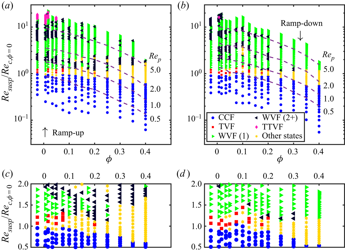
Figure 3. (a,b) A consolidated regime map as a function of particle volume fraction as well as suspension Reynolds number (normalized by the experimentally determined critical Reynolds number for single-phase flows,  $Re_{c,\phi =0} = 142$). In the legend, WVF (1) and WVF (2
 $+$) refer to periodic (single, distinct peak in the spectrum) and quasi-periodic (at least two, distinct, incommensurate peaks in the spectrum) wavy vortex flows, respectively. The single-phase flow case has been offset to aid better comparison. The purple dashed lines are approximate isolines for various particle Reynolds numbers. (c,d) Zoomed-in portion of the consolidated regime map corresponding primarily to the lower-order transitions.
This global overview already allows us to draw a few preliminary conclusions. In general, the critical suspension Reynolds number for the flow to display secondary structures decreases with increasing volume fraction of the solid particles, independent of the ramp direction. This observation is in agreement with recent experiments (Majji et al. Reference Majji, Banerjee and Morris2018; Ramesh et al. Reference Ramesh, Bharadwaj and Alam2019) as well as theoretical linear stability analysis (Ali et al. Reference Ali, Mitra, Schwille and Lueptow2002; Gillissen & Wilson Reference Gillissen and Wilson2019). This premature destabilization has been attributed to the anisotropy in the suspension microstructure, with neighbouring spheres interacting in the compressive direction of the base flow (Gillissen & Wilson Reference Gillissen and Wilson2019).
The major addition to the regime map is that the suspensions introduce what has been marked as ‘other states’, which usually precedes the wavy vortex flow (WVF) regime. These refer to the collection of states reported in recent literature, among others (wavy) spiral vortex flows (reported first by Majji et al. Reference Majji, Banerjee and Morris2018) as well as coexisting states (reported first by Ramesh et al. Reference Ramesh, Bharadwaj and Alam2019). Moreover, the range of Reynolds numbers over which these states are observed increase with increasing volume fraction for both ramp protocols. This results in increasing separation between circular Couette flow (CCF) and wavy vortex flows. This observation seems to be in agreement with the regime map of Ramesh et al. (Reference Ramesh, Bharadwaj and Alam2019), but not with that of Majji et al. (Reference Majji, Banerjee and Morris2018), who seemingly have the opposite trend.
There is a diminished appearance of axisymmetric Taylor vortex flow (TVF) as a standalone state, with increasing volume fraction, irrespective of our experimental protocol. This observation is in contrast to, both, Majji et al. (Reference Majji, Banerjee and Morris2018) and Ramesh et al. (Reference Ramesh, Bharadwaj and Alam2019). While Ramesh et al. (Reference Ramesh, Bharadwaj and Alam2019) observe Taylor vortices over a finite range of Reynolds numbers, irrespective of the particle volume fraction ( $\phi < 0.25$), Majji et al. (Reference Majji, Banerjee and Morris2018) observe that the range of Reynolds numbers over which Taylor vortices are obtained diminishes with increasing volume fraction (
 $\phi < 0.2$), while not observing the state altogether for
  $\phi = 0.30$. One possible reason for our lack of observation of Taylor vortices, as compared to other works, might be the nature of our experimental protocol, which has higher effective acceleration rates, as well as the limited amount of time spent at a constant Reynolds number. Majji et al. (Reference Majji, Banerjee and Morris2018) do observe in their transient studies that coexisting flow states that initially appear to have axial segregation, eventually develop into fully formed Taylor vortices after 5–10 min (see
  $Re = 116.9, 119.0$ in figure 15 of Majji et al. Reference Majji, Banerjee and Morris2018). The diminished appearance of Taylor vortices in our experiments prevents us from verifying the observation of Ramesh et al. (Reference Ramesh, Bharadwaj and Alam2019) whether the transition from Taylor vortices to wavy vortices is subcritical or not.
As far as higher-order transitions are concerned, the implications of the addition of particles are subtler. For example, the first appearance (or last, for ramp-down experiments) of wavy vortices may also be quasi-periodic, but a clear trend is not observed for the same. Moreover, as shall be seen later, the onset of chaos is delayed and the nature of transitions is seemingly qualitatively different from its single-phase flow counterpart. These flow regimes are explored in more detail by examining three volume fractions corresponding to different regimes of a suspension.
3.2. Torque measurements
The flow visualization measurements were complemented by global measurements of torque, which are often used to characterize flow regimes, be it from the perspective of rheology (Bagnold Reference Bagnold1954) or from turbulence (Eckhardt et al. Reference Eckhardt, Grossmann and Lohse2007). In figure 4 we show the consolidated  $Nu_{\omega }-Ta$ plot for all our ramp-up experiments. We note that between the suspension experiments and the single-phase flow experiments, the experimental set-up was dismantled and reassembled. For this reason, we do not consider the single-phase flow results in the empirical fitting. We emphasize that we do not account for effective suspension viscosity in either
  $Nu_{\omega }$ and
  $Ta$, as this allows us to easily interpret drag increase/reduction as an effect of the addition of particles.
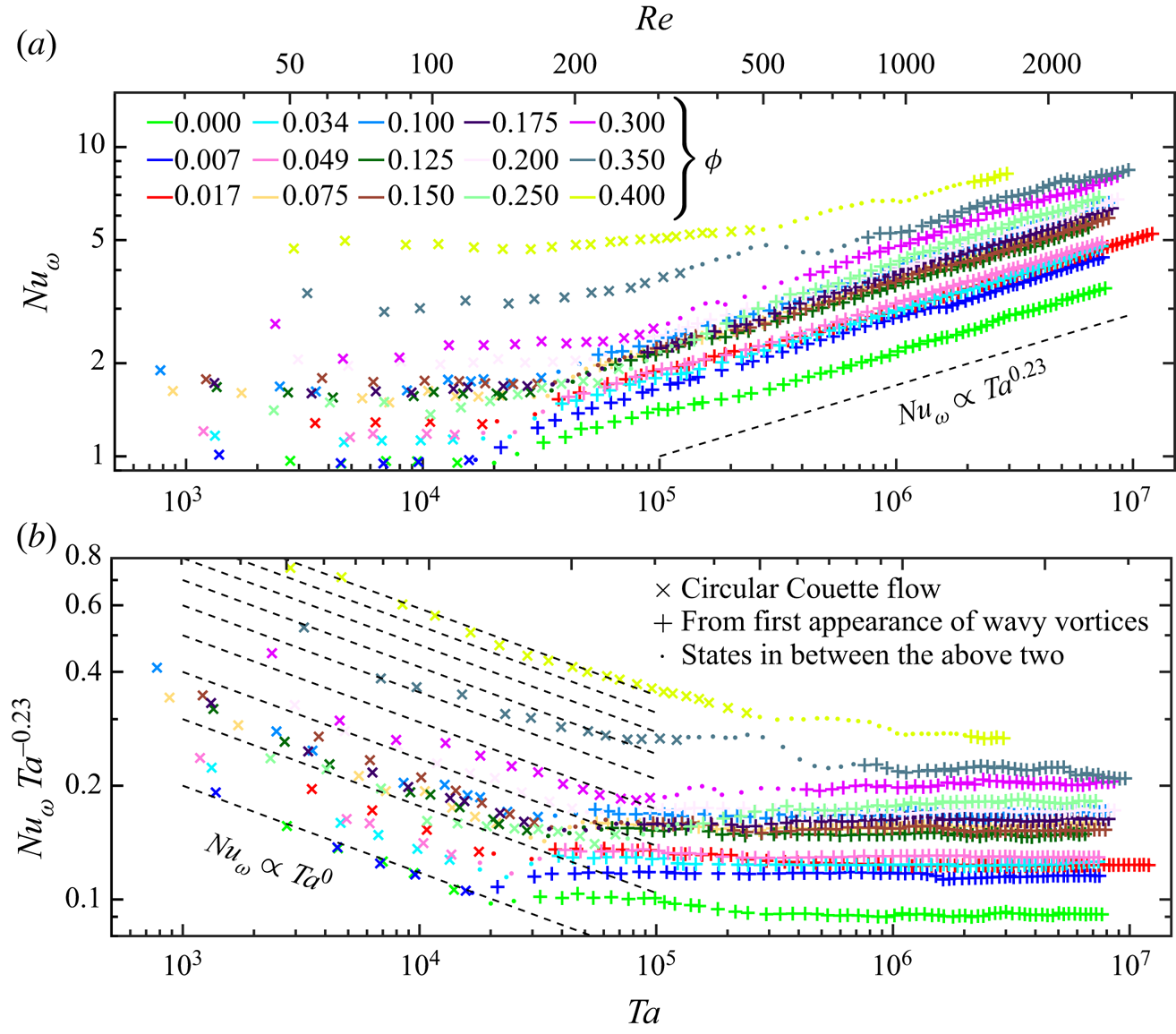
Figure 4. (Compensated)  $Nu_{\omega }-Ta$ scaling for all ramp-up experiments.
In figure 4 we distinguish the flow regimes into three: (i) CCF; (ii) intermediate states (corresponding to all points between CCF and WVF (1/2 $+$) in figure 3, often TVF and ‘other states’); and (iii) WVF onwards (all points from the first appearance of WVF, irrespective of the nature of the spectrum).
We first consider points corresponding to those classified under circular Couette flow (all crosses  $\times$ in figure 4). For all suspensions with
  $\phi \leq 0.20$, we observe that
  $Nu_{\omega }$ is independent of
  $Ta$. In rheological terms this simply means that the viscosity is independent of the shear rate, i.e. the flow behaviour is Newtonian. However, for
  $\phi \geq 0.25$, at higher
  $Ta$ (in the laminar regime), there is an increase in the scaling exponent which might be indicative of shear-thickening like effects. Picano et al. (Reference Picano, Breugem, Mitra and Brandt2013) attributed the ‘inertial’ shear-thickening to the presence of anisotropy in the microstructure of the non-colloidal suspension flow (
 $Re_p \in [0.4,40]$). This effect was caused by the presence of a shadow region, and the authors account for it by means of an ‘effective volume fraction’ (volume fraction after excluding the shadow regions).
From the onset of wavy vortices (all pluses  $+$ in figure 4), it was observed that
  $Nu_{\omega }$ scaled approximately with
  $Ta^{0.23}$. This is especially true for the dilute and semi-dilute suspensions. Only for the densest suspensions (
 $\phi \geq 0.25$) it was observed that the scaling exponent fluctuated in the range
  ${\pm }0.03$, without any clear trend. In a global sense, the exponent was
  $0.226 \pm 0.014$ (correspondingly,
  $\alpha = 1.45 \pm 0.03$ in
  $G \propto Re^{\alpha }$). Nevertheless, these fluctuations are subtler than the changes observed upon the onset of the fully developed turbulence regime characterized by a transition from laminar to turbulent boundary layers. For this transition, the coefficients are expected to gradually change from
  ${\sim }0.25$ to
  ${\sim }0.38$.
A similar observation was made in the experiments of Bakhuis et al. (Reference Bakhuis, Verschoof, Mathai, Huisman, Lohse and Sun2018) ( $\eta = 0.716$,
  $\varGamma = 11.7$), albeit at extremely high Reynolds numbers (
 $O(10^6)$) and lower volume fractions (
 $\phi \leq 0.08$), where only minimal changes in the scaling exponent were observed in their relation
  $Nu_{\omega } \propto Ta^{0.40}$. On the other end of the particle loading spectrum, the torque measurements of Savage & McKeown (Reference Savage and McKeown1983) (
 $\eta = 0.627$,
  $\varGamma = 5.08$) showed that the particle size had a greater impact on the scaling between shear stress and apparent strain rate than particle loading itself (
 $\phi > 0.4$,
  $Re \sim O(10^3)$). While not discussed explicitly, their measured shear stresses and apparent strain rates appear to be related by
  $\tau \propto \dot {\gamma }_{app}^{1.2\text {--}1.4}$ (i.e.
  $Nu_{\omega } \propto Ta^{0.1\text {--}0.2}$; see figure 7 in Savage & McKeown Reference Savage and McKeown1983). The relatively lower scaling exponents for Savage & McKeown (Reference Savage and McKeown1983) may be a result of the relatively small aspect ratio. While not reported explicitly by the authors, the exponent for the Taylor number appears to be a function of the particle volume fraction in the work of Ramesh et al. (Reference Ramesh, Bharadwaj and Alam2019) (see their figure 17), in contrast to our findings. For example, in their ramp-down experiments for
  $180 \geq Re_{{susp}} \geq 150$, it appears that
  $Nu_{\omega ,{susp}} \propto Ta^{0.26}_{{susp}}$ for
  $\phi = 0.10$ and
  $Nu_{\omega ,{susp}} \propto Ta^{0.35}_{susp}$ for
  $\phi = 0.20$.
Another telling observation in the current results is the nature of the curve itself or, more specifically, how the curve transitions from  $Nu_{\omega } \propto Ta^{0}$ to
  $Nu_{\omega } \propto Ta^{0.23}$. For the dilute suspensions, there is a relatively sharp shift between the two scaling exponents. However, for the densest suspensions, especially
  $\phi \geq 0.35$, the shift between the two scaling regimes is visibly gradual. Similar observations were visible in skin friction coefficient plots of recent particle-laden pipe flow experiments, and have been attributed to the presence/absence of turbulent puffs (Hogendoorn & Poelma Reference Hogendoorn and Poelma2018; Agrawal, Choueiri & Hof Reference Agrawal, Choueiri and Hof2019). Similar behaviour for particle-laden channel flows was demonstrated by Lashgari et al. (Reference Lashgari, Picano, Breugem and Brandt2014), by means of streamwise velocity fluctuations, which was attributed to inertial shear-thickening effects. Moreover, Ramesh et al. (Reference Ramesh, Bharadwaj and Alam2019) too observe this behaviour in their Taylor–Couette flow experiments (
 $\phi = 0.10, 0.20$). In the current case, this observation may be correlated with the separation between CCF and WVF (thus, all dots in figure 4). As shown previously in figure 3, the separation between CCF and WVF seemingly increased with increasing volume fraction of the particles, which may lead to the smoothness of the transition. Since correlation does not necessarily mean causation, this correlation should be revisited in the future.
As a final step in the torque data analysis, we assimilate our data into an empirical fit of the nature:  $Nu_{\omega } = B Ta^{k} \chi ^{e \, n}$. Here,
  $\chi ^{e}$ is the relative viscosity (Eilers’ fit:
  $\mu _{{susp}}/\mu = [1+1.25\phi /(1-\phi /0.614)]^{2}$).
We assume that drag augmentation in our experiments is brought upon solely by a rise in the effective viscosity. With the above expression, we implicitly neglect drag increase due to the formation of a particle-wall layer that has been observed in turbulent, particle-laden channel flows (Costa et al. Reference Costa, Picano, Brandt and Breugem2016). Such an assumption may be valid since the investigated flows in the current study are not turbulent, and, thus, the existence of a particle-wall layer may be questioned. Nevertheless, it must be noted that Sarabian et al. (Reference Sarabian, Firouznia, Metzger and Hormozi2019) report particle layering near both the cylinder walls in the circular Couette flow regime for  $0.20 \leq \phi \leq 0.50$ in their experiments with non-Brownian suspensions. The relative contributions of particle-wall layering and rise in effective viscosity to drag augmentation should be explored in the future.
We fit data corresponding to all particle-laden flows from the onset of wavy vortices (thus, all the pluses in figure 4, except  $\phi = 0$). We neglect the single-phase case for the fitting due to the aforementioned arbitrary correction employed, and this correction is expected to primarily affect the prefactor
  $B$, which is not of much interest. The results are tabulated in table 2. The fitted exponent for the Taylor number for the ramp-up experiments,
  $k$, is
  ${\sim}0.23$, in accordance with the visual observation of the scaling,
  $Nu_{\omega } \propto Ta^{0.23}$. The fitted exponents for the ramp-down experiments do not deviate significantly from the ramp-up ones.
Table 2. Coefficients (95 % confidence bounds in parentheses) obtained by a surface fit of data (all the pluses in figure 4, except  $\phi = 0$) to the equation
  $Nu_{\omega } = B Ta^{k} \chi ^{e \, n}$, as well as the corresponding R-square.

The scaling exponent of 0.23 corresponds to  $\alpha \sim 1.46$ (
 $G \propto Re^{\alpha }$). Eckhardt et al. (Reference Eckhardt, Grossmann and Lohse2007) provide an explanation for the physical origin of these scaling exponents for single-phase flows. An exponent of
  $\alpha \sim 1.5$ is attributed to the dominance of boundary layer and hairpin contributions to the transport of angular velocity, as compared to that from the bulk and the background. The authors also propose relationships for the thickness of the boundary layers, for the azimuthal velocity as well as axial velocity, relative to the gap width. For the range of Reynolds numbers studied here, it may be expected that the boundary layers are thick and occupy a large fraction of the annular gap width. The absence of deviation in the scaling exponent between
  $Nu_{\omega }$ and
  $Ta$ across all the volume fractions might suggest that the particles do not influence the nature of the angular momentum transfer between the cylinders (at least for the parameters studied here).
Another relevant non-dimensional number is the Bagnold number (Bagnold Reference Bagnold1954). The Bagnold number is the ratio between grain collision stresses to viscous stresses and, for all our experiments, it is found to be  $Ba < 40$, implying that all our experiments were in the so-called ‘macro-viscous regime’. Beyond
  $Ba > 450$, the grain collision stresses also play a major role and can shift the nature of the torque scaling significantly. Thus, despite our experiments spanning a wide range of suspension topologies, we do not notice a major impact on the scaling exponent, probably because all our experiments were in the ‘macro-viscous regime’. But again, it has also been reported that the Bagnold number is insufficient to distinguish contributions from turbulence and particles (Lashgari et al. Reference Lashgari, Picano, Breugem and Brandt2014), which highlights the complexity of explaining the observation.
In the end, even though the results are not completely unambiguous, we can still report an approximate empirical scaling law from our observations, which approximately reads as  $Nu_{\omega } \propto Ta^{0.24} \chi ^{e \, 0.41}$. Alternatively, this scaling behaviour may also be written as
  $G \propto Re^{1.49} \chi ^{e \, 0.41}$ or
  $c_f \propto Re^{-0.51} \chi ^{e \, 0.41}$. We reiterate that the above terms are defined using the fluid viscosity and not the suspension viscosity, except
  $\chi ^{e}$, and that this scaling is valid beyond the first appearance of wavy vortices.
4. Lower-order transitions: from circular Couette flow to the first appearance of wavy vortices
In this section we coarsely traverse the flow regimes studied exhaustively by Majji et al. (Reference Majji, Banerjee and Morris2018), Ramesh et al. (Reference Ramesh, Bharadwaj and Alam2019) and Ramesh & Alam (Reference Ramesh and Alam2020). All these studies performed their experiments at a very low ramp rate, in contrast to our experiments. We primarily intend to verify the existence of non-axisymmetric flow structures and coexisting states in our flow facility, which appear in the presence of particles. Thus, we perform a qualitative comparison with the findings in the above works. We also tested slower ramp rates in the limited range corresponding to the lower-order transitions, which are known to be especially sensitive to ramping protocols. This gave results similar to those obtained using ramp rates corresponding to our experiments.
As a reference, in single-phase flows, the flow transitions from circular Couette flow to laminar wavy vortex flow via Taylor vortex flow. By the first appearance of wavy vortices, we only consider patterns where the wave travels solely in the azimuthal direction and not axially. Thus, wavy spiral vortices are not considered as the demarcation between lower- and higher-order transitions.
4.1. Dilute suspension: detailed example of  $\phi = 0.034$

In general, the nature of the lower-order transitions for the dilute suspensions did not vary significantly from that of single-phase flows, in both experimental protocols. The first significant appearance of anomalies in our experiments occurs at  $\phi = 0.034$, slightly lower in comparison to
  $\phi = 0.05$ reported in other similar experiments (Majji et al. Reference Majji, Banerjee and Morris2018; Ramesh et al. Reference Ramesh, Bharadwaj and Alam2019), possibly owing to the difference in experimental protocols as well as higher particle Reynolds numbers.
Select regions of flow transitions for  $\phi = 0.034$ are shown in figure 5, primarily to demonstrate the differences from single-phase flow. In the ramp-up experiments the flow from CCF (
 $Re_{{susp}} = 118$) transforms to a state with a presence of mildly visible spirals with Taylor vortices towards the ends (
 $Re_{{susp}} = 134$). Hereafter, the flow transforms to a state with Taylor vortices barring a defect at the mid-height of the Taylor–Couette system (
 $Re_{{susp}} = 151$), which has a trident like shape on a space–time plot. We conjecture that there is a competition between the Taylor vortices arriving from the top and the bottom, and that this could possibly be a transient state. Hereafter, we observe a flow state seemingly developing into a fully wavy vortex flow (
 $Re_{{susp}} = 172$). This is visible in the space–time plot as a small portion of the Taylor vortices eventually transforms into wavy vortices (
 $Re_{{susp}} = 185$).
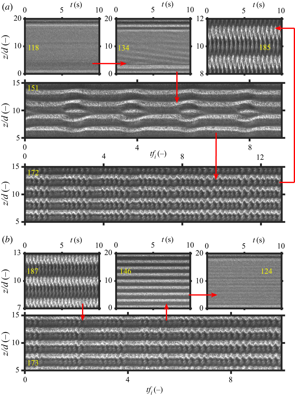
Figure 5. Lower-order transitions for a dilute suspension ( $\phi =0.034$). Only for the stretched space–time plots, the
  $x$-axis is time normalized by the time period of the inner cylinder rotation. The numbers in the figures represent the suspension Reynolds numbers,
  $Re_{{susp}}$. (a) Ramp-up experiments. (b) Ramp-down experiments.
The route for the ramp-down experiments is very similar to the ramp-up ones. We observe wavy vortex flow ( $Re_{{susp}} = 187$) devolve into Taylor vortex flow (
 $Re_{{susp}} = 146$) via a partially wavy vortex flow (
 $Re_{{susp}} = 173$). While in the ramp-up experiment it was observed that the waviness of the vortices grew in time, the same is observed here, while one might expect a slow devolution into a state entirely occupied by Taylor vortices. A possible reason is that the waviness (even partially occupying the system) may be considered as a destabilizing perturbation, which allows the wave to grow. The Taylor vortices are then suppressed upon reducing the shear rate (
 $Re_{{susp}} = 124$), and the flow is nearly free of secondary structures thereafter. It must be noted that the developing wavy vortices have not been reported either by Majji et al. (Reference Majji, Banerjee and Morris2018) or Ramesh et al. (Reference Ramesh, Bharadwaj and Alam2019). We revisit the flow state with developing wavy vortices in § 4.5.
4.2. Semi-dilute suspension: detailed example of $\phi = 0.15$

With increasing particle loading, it was noted in figure 3 that the gap separating CCF and WVF grew. We look into the example of a semi-dilute suspension, by considering the case of  $\phi = 0.15$. Examples of the lower-order transitions are shown in figure 6 for both experimental protocols.

Figure 6. Lower-order transitions for a semi-dilute suspension ( $\phi =0.150$). See caption of figure 5 for other details.
In the ramp-up experiments CCF ( $Re_{{susp}} = 117$) transforms into a state with a sharp distinction between the topologies in the top and bottom halves (
 $Re_{{susp}} = 132$). The top half has axisymmetric Taylor vortices, whereas the bottom half has non-axisymmetric spiral vortices. This flow topology is very reminiscent of the coexisting states reported recently by Ramesh et al. (Reference Ramesh, Bharadwaj and Alam2019). Upon increasing the shear rate (
 $Re_{{susp}} = 144, 152$), the overall flow topology remains unchanged, but the following can be observed. A very low-frequency waviness appears along the spiralling structure, accompanied by a crest on the Taylor vortices at the corresponding azimuthal location. A similar flow state was achieved in the transient evolution experiments of Majji et al. (Reference Majji, Banerjee and Morris2018) for their
  $Re_{{susp}} = 107.6$, a particle loading of
  $\phi = 0.10$ and particle diameter of
  $d_p = 230 \ \mathrm {\mu }\mathrm {m}$, which they describe as ‘a combination of spirals and Taylor vortices with azimuthal waviness’. Upon increasing the shear rate further, the segregation still persists, but a high-frequency waviness is now evident as well, with the inclination of the spirals slowly reducing (
 $Re_{{susp}} = 164, 178, 192$), until they are completely horizontal (
 $Re_{{susp}} = 201, 211$), with the absence of any structures travelling axially. The signature of the crests/defects appearing at lower Reynolds numbers (
 $Re_{{susp}} = 152$) are also the possible reason for the wavy vortices initially appearing distorted (
 $Re_{{susp}} = 201$). We observe wavy spirals at volume fractions as low as
  $\phi = 0.10$. This is in contrast with other similar experiments. For example, while Majji et al. (Reference Majji, Banerjee and Morris2018) begin to observe these structures only from
  $\phi \geq 0.20$, Ramesh et al. (Reference Ramesh, Bharadwaj and Alam2019) do not observe this flow regime altogether. Moreover, the wavy spirals observed by Majji et al. (Reference Majji, Banerjee and Morris2018) seemingly do not have any visible higher-frequency waviness, observed in the current experiments.
The ramp-down experiments, in contrast, show a relatively different behaviour. Wavy vortex flow ( $Re_{{susp}} = 197$), upon a reduction of shear (
 $Re_{{susp}} = 181$), devolves into a state similar to the developing wavy vortices also observed for
  $\phi = 0.034$. Upon further reduction of shear (
 $Re_{{susp}} = 166$), we observe a state with a mix of inclined vortices (with opposite inclinations either side of the mid-height), with wavy vortices occupying the circumference partially, possibly at the same locations of the partially developed wavy vortex flow state. Further reduction of the shear rate (
 $Re_{{susp}} = 155, 144$) led to a segregated state, wherein the region around the mid-height had spiralling structures while the ends had Taylor vortices. Similar observations have been made in counter-rotating, single-phase flow as well, with spirals existing between rotating defects (Hoffmann, Lücke & Pinter Reference Hoffmann, Lücke and Pinter2005). This served as a precursor to the formation of ribbons (
 $Re_{{susp}} = 130$), albeit fainter than those observed by Majji et al. (Reference Majji, Banerjee and Morris2018). We do not regularly observe ribbons structures, unlike Majji et al. (Reference Majji, Banerjee and Morris2018), possibly due to the pace of our experimental protocol, as well as the limited regions over which this flow state is found to be stable. The lowest volume fraction we observed ribbons was at
  $\phi = 0.075$. Then, the flow reaches CCF at
  $Re_{{susp}} = 117$.
4.3. Dense suspension: detailed example of $\phi = 0.30$

Finally, we consider an example of a dense suspension, namely  $\phi = 0.30$. It must be noted that the image quality begins to deteriorate with increasing volume fractions, and at the highest volume fractions studied (
 $\phi = 0.40$), visual analysis becomes less straightforward, possibly because the dispersed phase begins to block the optical path. Examples of lower-order transitions for
  $\phi = 0.30$ are shown in figure 7.
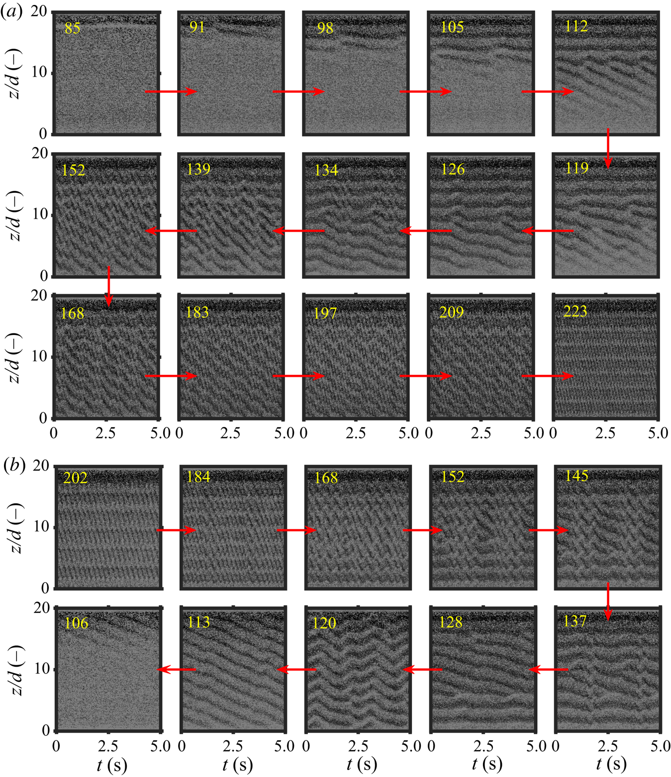
Figure 7. Lower-order transitions for a dense suspension ( $\phi =0.30$). An image adjustment procedure has been employed to enhance the contrast. See caption of figure 5 for other details.
The flow topologies for the ramp-up experiments qualitatively resemble the observations for  $\phi = 0.15$. The flow is azimuthal to begin with (
 $Re_{{susp}} = 85$), and the flow topology slowly evolves (
 $Re_{{susp}} = 91, 98, 105, 112$) until the secondary structures occupy the entire axial extent of the system (
 $Re_{{susp}} = 119, 126$). There are two noteworthy observations: firstly, a coexisting flow state is formed with Taylor vortices at the top and spiral vortices at the bottom, and secondly, that the flow requires a lot more time in order to go from a purely circular state to a flow with secondary structures. The latter might imply that the presence of particles in such large quantities suppresses the development rate of the flow state in time. Upon increasing the Reynolds number further (
 $Re_{{susp}} = 134, 139, 152, 168, 183, 197, 209$), we observe that the spiralling structures swallow one of the Taylor vortices, while also developing waviness. The Taylor vortices too display waviness simultaneously. Eventually, the wavy vortex flow state is obtained (
 $Re_{{susp}} = 223$). Majji et al. (Reference Majji, Banerjee and Morris2018) do not observe the wavy vortex flow regime for
  $\phi = 0.30$ and also mention that they observe only a sequence of non-axisymmetric flow states. While the latter observation is true for the present experiments too, the former observation may be attributed to the lower suspension Reynolds numbers (
 $Re_{{susp}} \approx 140$) achieved by Majji et al. (Reference Majji, Banerjee and Morris2018), compounded with our observation that the separation between CCF and WVF grows with increasing
  $\phi$. The reduced speed in the formation of structures also makes it less straightforward to demarcate whether the flow state should be considered as CCF or not.
The ramp-down experiments show a devolution also not drastically different from that seen for  $\phi = 0.15$. The initially wavy vortex flow state (
 $Re_{{susp}} = 202$) begins to show amplifications on the waves, at least partially (
 $Re_{{susp}} = 184$), and the amplifications occupy the entire circumferential extent upon further reduction of the shear rate (
 $Re_{{susp}} = 168$). This is followed by the appearance of spiralling structures near the mid-height of the set-up accompanied by a damping of the waviness (
 $Re_{{susp}} = 152, 145, 137$), and eventually, we obtain a state with spiral vortices in the centre surrounded by Taylor vortices at both ends (
 $Re_{{susp}} = 128$). At
  $Re_{{susp}} = 120$ an interesting flow state is observed which might appear to be wavy vortex flow at first sight, but actually is a state with competing spirals (left winding versus right winding). These structures appear to be visually similar to cross-spirals (Altmeyer & Hoffmann Reference Altmeyer and Hoffmann2010). Further reduction in the Reynolds number (
 $Re_{{susp}} = 113$) yields a flow state with spirals spanning the entire axial extent, and then subsequent disappearance of secondary structures
  $Re_{{susp}} = 106$.
4.4. Can coexisting regimes in ramp-up experiments be due to imperfect neutral buoyancy?
The following discussion is primarily heuristic in nature and stems from the observation that the ramp-up experiments display more radical axial segregation of flow regimes than the ramp-down ones. Similar observations are visible in the experiments of Ramesh et al. (Reference Ramesh, Bharadwaj and Alam2019), where their ramp-up experiments yielded the coexisting states, while the ramp-down experiments did not (see figures 5, 12–14 in their article). An exception to this trend was found in the experiments of Ramesh & Alam (Reference Ramesh and Alam2020) who reported axially segregated states in their ramp-down experiments too. Majji et al. (Reference Majji, Banerjee and Morris2018) circumvent this conundrum altogether by sticking to a ramp-down protocol, as they observed migration of particles towards the axial boundaries (see § 3.2 of their article) in the event of following a ramp-up protocol. Moreover, a common assumption in all relevant experiments (Majji et al. Reference Majji, Banerjee and Morris2018; Ramesh et al. Reference Ramesh, Bharadwaj and Alam2019; Ramesh & Alam Reference Ramesh and Alam2020), including the present work, is that particles are homogeneously distributed.
Shown in figure 8 is a contour plot of times needed for a homogeneous suspension to settle/rise by one gap width of the annulus, in a finite container. This is done so by calculating the settling velocity of a homogeneous suspension in a confined vessel  $v_{s,h} = v_{t} (1-\phi )^n$, where
  $v_{t} = (\rho _p/\rho _f-1)(gd_p^2/(18\nu ))$ is the terminal velocity of a single particle (Richardson & Zaki Reference Richardson and Zaki1954). For the range of density difference uncertainties in the current experiment, the particle terminal velocity based Reynolds number
  $\ll 0.2$, so
  $n = 4.65 + 19.5(d_p/d) = 5.82$. While estimating the settling velocities, we have taken the extreme scenario of using the highest observed temperature for determining the kinematic viscosity.
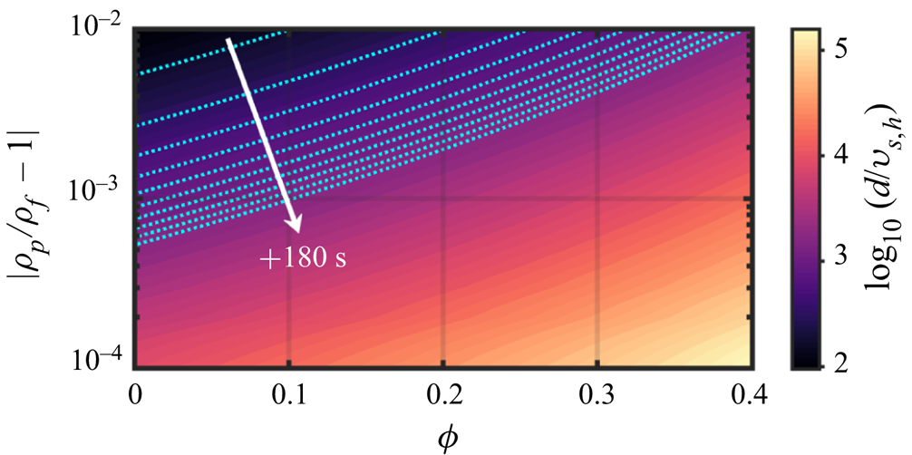
Figure 8. Estimated time duration needed for a homogeneous suspension to settle/rise by one gap width in a quiescent Taylor–Couette (for the current geometry) as a function of particle volume fraction and density mismatch. Each dotted blue line represents an isoline with increments of 180 s from 180 s to 1800 s.
For our ramp-up experiments, the flow was sheared at a very high rate before being left to rest for approximately 20 min prior to the commencement of experiments. After starting the experiments, typical durations before the flow developed any secondary structures were in the order of 5–10 min. Neglecting the influence of CCF on particle resuspension, the suspension gets approximately 30 min or 1800 s to non-homogenize. Since the estimated settling/rising velocities for marginal density differences are typically much smaller than velocities of secondary flow structures, the settling/rising effect may be neglected once secondary flow structures appear.
Assuming that the various uncertainties (including effect of temperature as well as particle density distribution) cause a density difference of 0.005 (0.5 %), then the suspension is able to axially migrate 3 gap widths, before the flow can develop secondary structures for  $\phi = 0.15$, and approximately 0.8 gap widths for
  $\phi = 0.30$, for example. These are relatively large distances and can result in inhomogeneous distribution of suspension Reynolds number across the axial direction. This in turn could cause different instability mechanisms across the axial direction, triggering the formation of axially segregated coexisting states.
In conclusion, it may be said with the help of the above estimates that the existence of ‘coexisting states’ with radical axial segregation of flow states could be affected by marginal density differences between the two phases. In virtually all experiments using large quantities of particles, these imperfections may be unavoidable. However, conclusively (dis)proving whether subtle density differences play a significant role would require simultaneous measurements of particle volume fractions along the axial direction.
4.5. Azimuthally localized wavy vortex flow: transient or a new regime?
A question that can be raised is whether the flow structures observed in the detailed examples here were spawned by our experimental protocol, which involves higher ramp rates ( $|\textrm {d}Re/\textrm {d}\tau | \sim O(1)$) as well as limited durations over which a constant Reynolds number was maintained (90 s). The transient evolution experiments of Majji et al. (Reference Majji, Banerjee and Morris2018) serve as a good reference for this matter (see figure 15 of their article). Over the short term (
 ${\sim }5\ \textrm {min}$), several of their experiments display coexisting states (axially segregated), and a few of these even survive for up to 30 minutes. Thus, these experiments do suggest that flows with axial segregation and/or defects may survive for extended periods of time. Even Chossat & Iooss (Reference Chossat and Iooss1994) state in their book, ‘For instance, for values of the parameters where spiral waves are expected, one actually sees a flow with “defects”, and one has to wait quite a long time before these defects disappear’. Thus, the same may be applicable to our experiments, and that a few of our reported flow states may be transients while a few of them might survive for an extended period of time.
One of the most intriguing flow states observed in our experiments was the developing/intermittent/localized wavy vortex flow ( $Re_{{susp}} = 172$, ramp-up in figure 5a;
  $Re_{{susp}} = 173$, ramp-down in figure 5b;
  $Re_{{susp}} = 181$, ramp-down in figure 6b). This state primarily differs from the flow states with defects, in the sense that there are no sinks/sources, and that any segregation occurs in the azimuthal direction (a fraction of the circumferential span has waviness on the otherwise axisymmetric Taylor vortices). These structures were observed in both the ramp-up as well as ramp-down experiments, ruling out any path dependence. The space–time plot on its own does not clarify whether this flow state is a combination of Taylor vortices and wavy vortices, coexisting at separate azimuthal sectors, or if the Taylor vortices become wavy for a short period of time before returning to the axisymmetric form.
In order to unveil the nature of these developing/intermittent/localized wavy vortex flows additional experiments were performed. The rotational frequency of the inner cylinder was manually adjusted until the desired flow state was achieved. Hereafter, the rotational frequency or the Reynolds number was kept constant (thus,  $|\textrm {d}Re/\textrm {d}\tau | = 0$). Imaging is performed with the help of three cameras (GoPro Hero 7 Black), simultaneously recording separate circumferential sectors of the Taylor–Couette system. Synchronization of the three cameras is done in the post-processing stage by identifying the time instant of a distinct sound source. Classical methods of visualizing the entire circumference of the Taylor–Couette system typically involves using multiple mirrors and a single camera (Gorman & Swinney Reference Gorman and Swinney1982; Prigent & Dauchot Reference Prigent and Dauchot2000). However, these were not pursued due to space constraints around our facility.
Shown in figure 9 is a schematic of the process depicting the transition between Taylor vortices and wavy vortices in suspension-laden systems. Intermediate states, i.e. waves only present partially across the circumference, are visible in two forms: a stable and an unstable form (see online supplementary material, movies 1 and 2, respectively). In our experiments this flow state is primarily observed in the transition process between Taylor vortex flow and wavy vortex flow. On multiple instances, we have observed this flow topology lasting for longer than an hour. Our longest observation of this flow state in a stable form has been in a suspension with  $\phi = 0.15$ for approximately 5 h (approximately 15 000 inner cylinder rotations). Towards the end of its lifetime, the wavy fraction slowly decayed to leave behind axisymmetric Taylor vortices. We have also observed scenarios where the wavy fraction grew in extent to occupy the entire circumference. It is also common to normalize the time with an advective time scale,
  $\dot {\gamma }_{{app}}^{-1}$, while studying transient structures (Borrero-Echeverry, Schatz & Tagg Reference Borrero-Echeverry, Schatz and Tagg2010). In such a case, the lifetime of the structure is
  ${\approx }1 \times 10^6$. The longevity of this flow state can be better tested in a temperature controlled facility, which truly allows for
  $|\textrm {d}Re/\textrm {d}\tau | = 0$.

Figure 9. Schematic representation of flow topologies when Taylor vortices transform into wavy vortices via a localized growth in a suspension-laden system. The red and blue (wavy) tori represent a pair of counter-rotating vortices with opposing azimuthal vorticity. For suspensions, it is also possible for the flow to stabilize at an intermediate state.
In figure 10 we present an example of a stable version of the azimuthally localized wavy vortex flow state. The two bottom panels prove the existence of the localized flow state for at least 1200 s. We estimate the wave speed to be approximately half the speed of the inner cylinder. The recipe to achieve a stable form of the localized wavy vortex flow state is still an open question. From our experience, an unstable version is easily achieved by setting a constant shear rate which corresponds to a Reynolds number slightly above the critical value needed to obtained wavy vortices. The stable version has usually been achieved by arbitrarily varying the shear rate at the boundary between Taylor and wavy vortices, crossing it on multiple occasions. The stable version shown here was attained at  $Re_{{susp}}/Re_{c,\phi =0} \approx 1.54$ for
  $\phi = 0.10$. For reference (see figure 3), the transition between wavy vortex flow and the preceding (succeeding, alternatively) flow state occurs between
  $1.20 \leq Re_{{susp}}/Re_{c,\phi =0} \leq 1.28$ (
 $1.60 \geq Re_{{susp}}/Re_{c,\phi =0} \geq 1.44$) for the ramp-up (ramp-down) experiments.

Figure 10. An example of a sustained version of localized wavy vortex flow in a suspension with  $\phi = 0.10$. Coloured patches in the top panel (a) indicate the locations, where the scattered light intensity is sampled. The panels (b and c) are time series of the light intensity at three locations, close to the mid-height, recorded on the three individual cameras. Arrows in (b,c) indicate the propagation of the localized wave along the circumference. The time series in panels (b and c) are separated by 20 min. Our longest observation of this flow state has been in a suspension with
  $\phi = 0.15$ for approximately
  $t \approx 5\ \textrm {h}$. This corresponds to
  $tf_i \approx 15\,000$ or
  $t \dot {\gamma }_{{app}} \approx 1 \times 10^6$.
To the best of our knowledge, this specific flow state has not been reported in the past, even though similar observations have been made. We note that Ramesh et al. (Reference Ramesh, Bharadwaj and Alam2019) do identify a coexisting state with Taylor vortices and wavy vortices in suspension-laden flows, however with axial segregation. Moreover, Abshagen et al. (Reference Abshagen, von Stamm, Heise, Will and Pfister2012) report a flow state with an axial localization of an azimuthally rotating wave in single-phase flows. While the localized wavy vortex flow from our experiments appears to be similar to the ‘very short wavelength bursts’ reported by Carey, Schlender & Andereck (Reference Carey, Schlender and Andereck2007), the latter appears much beyond the onset of wavy vortex flow in high radius ratio systems. Wiener & McAlister (Reference Wiener and McAlister1992) also observed a solitary wave travelling across a system with axisymmetric Taylor vortices, but in the axial direction, while also reflecting off the end caps. Finally, an extremely similar flow state was reported in numerical studies on a rotating planar Couette flow by Salewski, Gibson & Schneider (Reference Salewski, Gibson and Schneider2019). A localized slug of wavy vortex flow emerged in a background of Taylor vortices via a modulational sideband instability. However, the localization occurred along the spanwise direction (axial direction in Taylor–Couette geometry) rather than the streamwise direction (azimuthal direction in Taylor–Couette geometry).
The transition between Taylor vortex flow and wavy vortex flow in single-phase flows has been attributed to the ‘self-sustaining process’ also known as the ‘regeneration cycle’ (Martinand, Serre & Lueptow Reference Martinand, Serre and Lueptow2014; Dessup et al. Reference Dessup, Tuckerman, Wesfreid, Barkley and Willis2018). Recent numerical work by Wang, Abbas & Climent (Reference Wang, Abbas and Climent2018) shed light on the regeneration cycle for the flow of (semi-)dilute suspensions comprised of neutrally buoyant, finite-size, spherical particles in a planar Couette flow as well as channel flow. A key conclusion was that the spatial distribution of the particles was decisive, whether they are predominantly present in the streamwise rolls or the streaks. We thus conjecture that the particles interfere with the self-sustaining process in our experiments, giving birth to this localized flow state, but proving this requires further investigation.
In conclusion, based on our observations, we can conclude that the azimuthally localized wavy vortex flow state might be either a stable state or a long-lived transient. Since we are unable to conclusively claim that this flow state has an infinite lifetime, there is a possibility that it may be a long-lived transient. We can nonetheless propose that finite-sized particles, which are known to cause premature destabilization of the flow, are also capable of inhibiting the growth of instabilities.
5. Higher-order transitions: from the first appearance of wavy vortices
In this section we discuss the nature of higher-order transitions in particle-laden flows. For the sake of simplicity, we classify the flows only as periodic or quasi-periodic, depending on the number of incommensurate peaks appearing in the spectrum. A periodic flow has a single, distinctly identifiable peak in the spectrum, while a quasi-periodic flow has multiple, incommensurate, distinctly identifiable peaks in the spectrum. As a reference, in single-phase flows the flow transitions roughly in the following order with increasing Reynolds number: laminar wavy vortex flow (periodic), modulated wavy vortex flow (quasi-periodic), chaotic wavy vortex flow (quasi-periodic), turbulent wavy vortex flow (periodic), turbulent Taylor vortex flow (aperiodic). The flow patterns including and beyond chaotic wavy vortex flows additionally feature small-scale structures. A caveat, however, is that the exact nature of higher-order transitions is not set in stone. The supplementary material includes a detailed example for single-phase flows, and provides an in-depth explanation of the terminology.
The primary tool we employ in this section is a simple spectral analysis along the time axis of the space–time plots. The spectra along each axial location are averaged to return a single spectrum. The averaging is not expected to be detrimental as fundamental frequencies have been found to be independent of the axial location (Fenstermacher et al. Reference Fenstermacher, Swinney and Gollub1979), even though this might not hold true for the amplitudes. Peaks in the spectra are identified as follows. All points at least ten median average deviations away from the median of the spectrum are marked as ‘potential peaks’. Hereafter, only the ‘potential peaks’ that are local maxima in the neighbourhood of five points are retained as true peaks. After isolating the true peaks, we use a mix of qualitative (visual inspection of the space–time plot) and quantitative conventions to classify the flow as either periodic or quasi-periodic. The quantitative approach is as follows: let  $p_1$ be the tallest peak,
  $p_2$ be the second tallest one and
  $p_b$ be the median of the spectrum + 10
 $\times$median average deviations. If the quantity
  $(p_1-p_b)/(p_2-p_b) < 10$ then we classify the flow as quasi-periodic. The frequencies in the spectra are normalized by the rotational frequency of the inner cylinder (
 $f_i$). Thus, all peaks close to
  $f/f_i = 1$ may be associated with the system itself. We also do not perform an extremely detailed, quantitative analysis of the spectra (for example, identifying the significance of different peaks, and identifying all the linear combinations), as it is not trivial (as evidenced by Gorman, Reith & Swinney Reference Gorman, Reith and Swinney1980; Takeda et al. Reference Takeda, Fischer, Sakakibara and Ohmura1993, in table 3 and figure 2, respectively) while also going beyond the scope of the current study.
While a similar spectral analysis can also be performed along the space axis to yield axial wavenumbers, we restrict our discussion to the (de)generation of vortex pairs (also referred to as vortex pinching/splitting processes by King & Swinney Reference King and Swinney1983). Given that our system has two fixed end plates, which fix the boundary conditions for the flow, the (de)generation of vortices in the axial direction only occurs in pairs. If the total integer number of waves encompassing the circumference,  $m$, is known with absolute certainty, then the wave speed (normalized with the inner cylinder speed) can be estimated as
  $\bar {c} = (\,f/f_i)/m$ (King et al. Reference King, Li, Lee, Swinney and Marcus1984). We can estimate
  $m$ by extrapolating from the full field-of-view snapshots. However, this approach is suspect to errors, which could affect the accurate determination of the wave speeds.
5.1. Dilute suspension: detailed example of $\phi = 0.034$

Firstly, we consider the example of  $\phi = 0.034$ in figure 11 to qualitatively probe the nature of the higher-order transitions in dilute suspensions. In the ramp-up experiments ‘other states’ are observed between
  $1.03 \leq Re_{{susp}}/Re_{c,\phi } \leq 1.32$. This is followed by wavy vortex flow for
  $1.42 \leq Re_{{susp}}/Re_{c,\phi } \leq 1.84$. Hereafter, between
  $1.92 \leq Re_{{susp}}/Re_{c,\phi } \leq 2.20$ the azimuthal waves undergo distortion, resulting in noisier spectra, and pave the way for a new flow state with different axial/azimuthal wavenumbers at
  $Re_{{susp}}/Re_{c,\phi } = 2.36$. This behaviour is similar to that observed in single-phase flows. This new wavy state with a single frequency component of
  $f/f_i \approx 3.8$ is sustained in the region
  $2.36 \leq Re_{{susp}}/Re_{c,\phi } \leq 6.16$. This is followed by flow states similar to modulated wavy vortex flow and/or chaotic wavy vortex flow for
  $6.46 \leq Re_{{susp}}/Re_{c,\phi } \leq 8.80$, characterized by the appearance of finer structures in the flow (suggesting presence of chaos) as well as spectra with multiple peaks. The flow then returns to a state characterized by a single, dominant frequency, while also displaying chaotic elements for
  $9.18 \leq Re_{{susp}}/Re_{c,\phi } \leq 13.03$ (barring
  $Re_{{susp}}/Re_{c,\phi } = 11.94$, when there is a shift in azimuthal wavenumbers), reminiscent of the wavy turbulent vortex flow in single-phase flows. The flow undergoes a spectral cascading process between
  $13.42 \leq Re_{{susp}}/Re_{c,\phi } \leq 14.1$, leading to a shift in the azimuthal wavenumber from
  $f/f_i \approx 2.3$ to
  $f/f_i \approx 1.9$. From
  $Re_{{susp}}/Re_{c,\phi } = 15.31$ to
  $Re_{{susp}}/Re_{c,\phi } = 15.61$, there is a sudden shoot-up in the frequency component from
  $f/f_i \approx 1.9$ to
  $f/f_i \approx 3.8$, which is sustained until the highest Reynolds number (
 $Re_{{susp}}/Re_{c,\phi } = 18.21$). A similar observation was made in our single-phase flow experiments, and could be likened to the ‘fast azimuthal wave’. Originally, this structure resembling the ‘fast azimuthal wave’ was reported to appear only after the appearance of turbulent Taylor vortices (Takeda Reference Takeda1999). In this sense, our observations may be likened to the findings of Imomoh, Dusting & Balabani (Reference Imomoh, Dusting and Balabani2010), who also observed this structure before the appearance of turbulent Taylor vortices.

Figure 11. Compilation of frequency spectra for a dilute suspension ( $\phi = 0.034$). Here
  $Re_{c,\phi }$ is the highest suspension Reynolds number at which circular Couette flow is identified. The size of the markers are proportional to their prominence in the spectrum. The dashed red lines approximately represent the primary frequency. A sudden drop (rise, respectively) in the dashed red line suggests a decrease (an increase) in the number of azimuthal waves. The coloured markers at the bottom correspond to the flow regimes shown in figure 3. (a) Ramp-up experiments. (b) Ramp-down experiments.
The ramp-down experiments initially return a flow state akin to the wavy turbulent vortex flow, characterized by a single, dominant frequency in the spectrum and fine-scale structures in the flow between  $15.11 \geq Re_{{susp}}/Re_{c,\phi } \geq 9.29$ (with the disappearance of a vortex pair at
  $Re_{{susp}}/Re_{c,\phi } = 12.14$). This is followed by a flow state with multiple, incommensurate frequencies in the spectra between
  $9.09 \geq Re_{{susp}}/Re_{c,\phi } \geq 7.97$, with the flow still displaying smaller-scale structures. This is then followed by wavy vortex flow between
  $7.63 \geq Re_{{susp}}/Re_{c,\phi } \geq 4.40$, characterized by a single dominant frequency (except
  $Re_{{susp}}/Re_{c,\phi } = 6.18$, when the azimuthal wavenumber undergoes a shift) and a gradually diminishing presence of finer flow features. Between
  $4.14 \geq Re_{{susp}}/Re_{c,\phi } \geq 3.34$, the flow appears to be similar to the early modulated wavy vortex flow and also precedes the appearance of wavy vortex flow with a new azimuthal state (from
  $f/f_i \approx 3.1$ to
  $f/f_i \approx 3.5$) as well as an axial one (reduction of a vortex pair). The flow then is wavy in nature for
  $3.12 \geq Re_{{susp}}/Re_{c,\phi } \geq 1.44$. A surprising observation is the creation of two vortex pairs between
  $1.87 \geq Re_{{susp}}/Re_{c,\phi } \geq 1.65$. This is then followed by an ‘other state’ (
 $Re_{{susp}}/Re_{c,\phi } = 1.33$) and Taylor vortex flow (
 $Re_{{susp}}/Re_{c,\phi } = 1.12$), before becoming purely circular.
5.2. Semi-dilute suspension: detailed example of $\phi = 0.15$

Next, we consider the example of a semi-dilute suspension using the case  $\phi = 0.15$ in figure 12. As seen in the section describing the lower-order transitions, proper wavy vortices are not observed in the ramp-up experiments until
  $Re_{{susp}}/Re_{c,\phi } = 1.63$ with
  $f/f_i \approx 3.5$, and this flow state persists until
  $Re_{{susp}}/Re_{c,\phi } = 1.87$. Between
  $1.87 \leq Re_{{susp}}/Re_{c,\phi } \leq 2.62$, the flow transitions to a state with wavy vortices, albeit with a different azimuthal wavenumber (reflected in
  $f/f_i \approx 3.8$), and with the loss of a vortex pair. This transition occurs with the appearance of distortion on parts of the waves (at
  $Re_{{susp}}/Re_{c,\phi } = 2.06$), which then give rise to a flow state with dislocations appearing in the form of wavy spiral vortices. Even for single-phase flows, splitting/merging of vortex pairs in the axial direction occurs by means of spiralling structures. Thus, it is fathomable that these spiralling structures are in fact intermediate states, and if more time were spent at each of the Reynolds numbers, the spiral might not have survived. Nevertheless, this observation throws weight behind our proposition that the presence of particles could lead to a reduction in the growth rate of instabilities. Hereafter, the flow states primarily sustain their waviness even until the highest Reynolds numbers we achieved
  $2.62 \leq Re_{{susp}}/Re_{c,\phi } \leq 13.91$. Moreover, the waviness usually has a single dominant frequency and quasi-periodicity is primarily observed when there is a shift in the azimuthal wavenumber. While not shown here, the spectra begin to appear noisier beyond
  $Re_{{susp}}/Re_{c,\phi } \geq 7.89$, while the flow also appears to display finer structures beyond
  $Re_{{susp}}/Re_{c,\phi } \geq 9.69$. Thus, the transition to chaos appears more vague compared to single-phase flows as it is not preceded by a flow state with two distinct, incommensurate frequencies. It may be concluded that the presence of higher number of particles can inhibit the appearance of the second, incommensurate frequency.

Figure 12. Compilation of frequency spectra for a semi-dilute suspension ( $\phi = 0.15$). See caption of figure 11 for other details.
The ramp-down experiments start of with a flow state with waviness, characterized by a spectrum with a single, dominant frequency ( $f/f_i \approx 2.2$) while also being amply noisy. The flow itself appears to have smaller-scale structures, and, thus, the flow may initially be chaotic. We note that in the ramp-down experiments, the Reynolds number initially increases from
  $Re_{{susp}}/Re_{c,\phi } = 10.65$ to a maximum of
  $Re_{{susp}}/Re_{c,\phi } = 10.77$, despite decreasing shear rates. This is caused by sharp reductions in the viscosity arising from viscous heating. Nevertheless, this wavy flow state is sustained for
  $Re_{{susp}}/Re_{c,\phi } \geq 8.24$. Between
  $8.05 \geq Re_{{susp}}/Re_{c,\phi } \geq 7.00$, the spectrum has multiple peaks, reminiscent of the chaotic wavy vortex flow state in single-phase flows. We note that such a flow state was not observed in the corresponding ramp-up experiments. Between
  $6.77 \geq Re_{{susp}}/Re_{c,\phi } \geq 1.59$, the flow is wavy, predominantly with a single frequency component (
 $2.5 \leq f/f_i \leq 3.7$), with the exception of
  $Re_{{susp}}/Re_{c,\phi } = 2.76, 2.57$, where the space–time plots appear similar to the early modulated wavy vortex flow seen for single-phase flows. The ‘other states’ are obtained between
  $1.46 \geq Re_{{susp}}/Re_{c,\phi } \geq 1.05$, before the flow becomes purely circular in nature.
5.3. Dense suspension: detailed example of $\phi = 0.30$

Finally, we consider an example of a dense suspension,  $\phi = 0.30$ in figure 13. The lower-order transitions, as shown previously, consisted primarily of the ‘other states’ (
 $1.06 \leq Re_{{susp}}/Re_{c,\phi } \leq 1.99$), before wavy vortices are obtained. However, as can be noticed from the compilation of spectra from the ramp-up experiments, the initial appearance of wavy vortices is accompanied by the presence of a secondary frequency (
 $\,f/f_i \approx 1.25$). This behaviour persists for
  $2.12 \leq Re_{{susp}}/Re_{c,\phi } \leq 2.92$. Moreover, between
  $2.80 \leq Re_{{susp}}/Re_{c,\phi } \leq 2.92$, additional apparent modulations are clearly visible on the space–time diagrams (visible as additional peaks in the spectra, near the primary peak
  $f/f_i \approx 4$), which then give way to a wavy vortex flow regime characterized by a single peak for the remainder of the experiments (
 $3.10 \leq Re_{{susp}}/Re_{c,\phi } \leq 8.88$), with the exception of locations where the flow transitions from one wavy state to another (
 $Re_{{susp}}/Re_{c,\phi } = 5.53, 6.62$). Curiously, between
  $5.69 \leq Re_{{susp}}/Re_{c,\phi } \leq 8.88$, a peak with a low amplitude (relative to the primary peak) is persistently present at
  $f/f_i \approx 3$. This also appears to be independent of the value of the primary frequency which varies from
  $3.1 \geq f/f_i \geq 2.3$. A key difference here from the single-phase flows is the lack of an extended region with a second, incommensurate frequency, which also has implications for the onset of chaos. A similar behaviour was also observed for
  $\phi = 0.15$. Thus, it indeed appears that the presence of particles inhibits the appearance of the second, incommensurate frequency. The peak at
  $f/f_i \approx 3$ seems to be the sole feature that may insinuate the appearance of a second frequency component, but we disregard it given its lack of strength. Of course, the studied range of Reynolds numbers (
 $Re_{{susp}}/Re_{c,\phi } \leq 8.88$) disallows us from drawing a firm conclusion on this matter, and can be a topic of interest in the future. In our single-phase flow experiments the wavy turbulent vortex flow state was attained at
  $Re/Re_{c} = 9.00$, preceded by flow regimes with apparent chaos. Thus, even though the presence of particles causes a premature appearance of secondary flows, their presence possibly delays the onset of chaos.

Figure 13. Compilation of frequency spectra for a dense suspension ( $\phi = 0.30$). See caption of figure 11 for other details.
The ramp-down experiments produce even less complicated transitions, and the dominant flow state is the wavy vortex flow between  $7.16 \geq Re_{{susp}}/Re_{c,\phi } \geq 1.92$. The flow eventually transitions back to ‘other states’ via wavy flow states with multiple incommensurate frequencies (
 $1.75 \geq Re_{{susp}}/Re_{c,\phi } \geq 1.60$). This is clearly visible in the space–time plots for
  $Re_{{susp}} = 178, 162$ in figure 7. Similar to the ramp-up experiments, an extremely weak peak is also present at
  $f/f_i \approx 3$ for
  $7.16 \geq Re_{{susp}}/Re_{c,\phi } \geq 4.31$. However, its significance remains unclear.
In conclusion, based on the three detailed examples considered here, we can claim that higher-order transitions in dilute suspensions are not qualitatively different from single-phase flows. However, with increasing particle volume fractions, there is evidence for the suppression of a second, incommensurate frequency. This frequency is commonly observed in single-phase flows (usually implying modulated waves) and serves as a precursor to the arrival of chaos (Gollub & Swinney Reference Gollub and Swinney1975; Fenstermacher et al. Reference Fenstermacher, Swinney and Gollub1979). The inhibition of the second, incommensurate frequency implies that at higher particle loadings, the route to chaos is altered.
6. Conclusions and outlook
In this section we summarize the key findings and their implications in § 6.1 and propose possible future investigations to extend upon the current study in § 6.2.
6.1. Summary of key findings
We set off with the target of addressing the following: previously unreported anomalies in lower-order transitions; nature of higher-order transitions; and the possibility to derive an empirical scaling law for the torque measurements. All these targets were in the context of experimentally studying neutrally buoyant, non-Brownian, particle-laden suspensions (solid spheres dispersed in a liquid) in a vertical Taylor–Couette geometry, driven by a rotating inner cylinder. The varied parameters include particle loading ( $\phi \in [0 \ 0.40]$), the (suspension) Reynolds number (up to
  $O(10^3$), by varying the apparent shear rate) as well as experimental protocol (increasing and decreasing Reynolds numbers). The key findings are listed below.
(i) Despite higher acceleration/deceleration rates (table 1), previously reported non-axisymmetric flow regimes (such as spirals and ribbons) as well as ‘coexisting states’ (constituted of two separate states axially segregated) are observed in the particle-laden flows. These are observed as a part of the lower-order transitions for suspensions (figures 5–7). Moreover, we identify that particle-laden flows are likelier to display ‘defects’.
(ii) We speculate in § 4.4 that ‘coexisting states’ (axial segregation of flow states) could potentially arise due to imperfect satisfaction of the neutral buoyancy. This stemmed from the observation that experiments with increasing Reynolds numbers in time, display radical segregation in flow states more often. Conclusively (dis)proving the above proposition would require accurate measurements of particle volume fraction profiles along the axial direction.
(iii) A novel flow regime is reported in the form of an azimuthally local wavy vortex flow, with a fraction of the circumference composed of Taylor vortices and the remainder being wavy (see figures 9 and 10). It may be considered as a ‘coexisting state’, with segregation in the azimuthal direction. Based on our observations, it is either a stable state or a long-lived transient.
(iv) Based on the increased appearance of defect-laden flow patterns as well as an example of a sustained azimuthally localized wavy vortex flow, we propose that the presence of a dispersed phase, which is known to trigger premature destabilization, is also capable of inhibiting the growth rate of instabilities. This is also proposed in the framework of the particles interfering with the self-sustaining process.
(v) The gap between circular Couette flow and the appearance of wavy vortices clearly increases with increasing particle loading (figure 3). Moreover, the first appearance of wavy vortices is sometimes quasi-periodic in nature, predominantly for dense suspensions undergoing ramp-up experiments.
(vi) Flow topologies corresponding to higher-order transitions in dilute suspensions are qualitatively similar to those observed in single-phase flows (figure 11). At the higher particle loadings, though, there are indications that the route to chaos is altered. This is based on the absence of a clear, second, incommensurate frequency (figures 12 and 13). This at least holds for the range of Reynolds numbers studied here.
(vii) We obtain an empirical scaling law from our torque measurements, which reads as
$Nu_{\omega } \propto Ta^{0.24} \chi ^{e \, 0.41}$ (figure 4 and table 2). This is valid for all our measurement points beyond the first appearance of wavy vortices, or for higher-order transitions in our study.

6.2. Possible future investigations
Given that the study of inertial instabilities in neutrally buoyant, non-Brownian, particle-laden Taylor–Couette flow is in a relatively nascent phase, a wide variety of questions can still be addressed experimentally in the future. This manuscript focused on characterizing flow transitions by evaluating global quantities, such as torque and classifying the flow regimes based on flow visualization. Commonly, changes in global quantities are intimately linked with changes in the microstructure of the flow. This alludes to the need for understanding the microstructure of the flow, which would consist of the velocities of the two phases as well as inhomogeneities in the spatial distribution of the dispersed phase. In fact, advances along this line have recently been made in understanding the internal properties of the flow structures (Ramesh et al. Reference Ramesh, Bharadwaj and Alam2019), enhanced mixing by particles (Dherbécourt et al. Reference Dherbécourt, Charton, Lamadie, Cazin and Climent2016; Rida et al. Reference Rida, Cazin, Lamadie, Dherbécourt, Charton and Climent2019) as well as radial migration of particles (Majji & Morris Reference Majji and Morris2018; Sarabian et al. Reference Sarabian, Firouznia, Metzger and Hormozi2019).
Even though this study aimed at expanding the studied parameter space, there still are several uncharted territories. For example, even higher Reynolds numbers ( $Re_{{susp}} \sim O(10^4)$) can be accessed, in order to assess the effect of particles on the onset of ultimate turbulence. Moreover, rotating the outer cylinder should also be a tantalizing prospect, given that counter-rotating single-phase Taylor–Couette flows are known to have non-axisymmetric modes arising as primary instabilities (Krueger, Gross & Di Prima Reference Krueger, Gross and Di Prima1966). Torque measurements can also allow for determining ‘optimal’ conditions, characterized by the ratio between the rotation rates of the two cylinders at which the transport of angular momentum between the cylinders is maximized (van Gils et al. Reference van Gils, Huisman, Grossmann, Sun and Lohse2012).
On the other hand, state-of-the-art, fully resolved numerical simulation techniques for particle-laden flows (de Motta et al. Reference de Motta, Costa, Derksen, Peng, Wang, Breugem, Estivalezes, Vincent, Climent and Fede2019) can complement measurements by state-of-the-art experimental techniques (Poelma Reference Poelma2020) and provide a deeper understanding of the underlying physical mechanisms.
Acknowledgements
We would like to thank A. Greidanus for accelerating the start-up of this project as well as J. Graafland, E. Overmars and J. Ruijgrok for their technical assistance with the experiments. Furthermore, we are grateful to W.-P. Breugem, G. Elsinga and W. van de Water for their valuable comments on an earlier version of the manuscript. A.D. and C.P. have received funding from the ERC Consolidator Grant 725183 ‘OpaqueFlows’.
Declaration of interest
The authors report no conflict of interest.
Supplementary material and movies
Supplementary material and movies are available at https://doi.org/10.1017/jfm.2020.649.


 Open access