Accelerating the Finite-Element Method for Reaction-Diffusion Simulations on GPUs with CUDA
by
 , and
, and
Hedi Sellami
1, 
Leo Cazenille
2,
Teruo Fujii
3,
Masami Hagiya
1,
Nathanael Aubert-Kato
2,* and
Anthony J. Genot
3,* 1
Department of Computer Science, The University of Tokyo, Tokyo 113-8654, Japan
2
Department of Information Sciences, Ochanomizu University, Tokyo 112-8610, Japan
3
LIMMS/CNRS-IIS, UMI2820, The University of Tokyo, Tokyo 153-8505, Japan
*
Authors to whom correspondence should be addressed.
Micromachines 2020, 11(9), 881; https://doi.org/10.3390/mi11090881
Submission received: 1 August 2020
/
Revised: 31 August 2020
/
Accepted: 3 September 2020
/
Published: 22 September 2020
(This article belongs to the Special Issue Recent Advances of Molecular Machines and Molecular Robots)
Abstract
:DNA nanotechnology offers a fine control over biochemistry by programming chemical reactions in DNA templates. Coupled to microfluidics, it has enabled DNA-based reaction-diffusion microsystems with advanced spatio-temporal dynamics such as traveling waves. The Finite Element Method (FEM) is a standard tool to simulate the physics of such systems where boundary conditions play a crucial role. However, a fine discretization in time and space is required for complex geometries (like sharp corners) and highly nonlinear chemistry. Graphical Processing Units (GPUs) are increasingly used to speed up scientific computing, but their application to accelerate simulations of reaction-diffusion in DNA nanotechnology has been little investigated. Here we study reaction-diffusion equations (a DNA-based predator-prey system) in a tortuous geometry (a maze), which was shown experimentally to generate subtle geometric effects. We solve the partial differential equations on a GPU, demonstrating a speedup of ∼100 over the same resolution on a 20 cores CPU.
1. Introduction
In the past two decades, the architecture of Graphical Processing Units (GPUs) have made them the tool of choice in scientific computing to solve massively parallel problems [1,2]. CPUs spend a sizable fraction of their transistors budget on caching and control units. This allows CPUs to quickly serve data that are often accessed (e.g., for database server) and to handle complex and varied flows of instructions (e.g., out-of-order or speculative execution), but this comes at a cost of a reduced number of computing units (arithmetic logic units). By contrast, GPUs spend almost all their transistor budget on arithmetic logic units, because they were initially designed to handle homogeneous but massively parallel flows of instructions (typically the rendering of graphical scenes, which heavily relies on linear algebra). This focus on computing units enables GPUs to beat CPUs on problems that can be formulated in a parallel manner. For instance, GPUs typically accelerate dense matrix multiplication (a classical, though somewhat artificial, benchmark for supercomputers) by a factor of 6 over CPUs [3], and most supercomputers now embark GPUs to accelerate their computations.
This speedup comes at a cost: it is necessary to write specific code to fully exploit the parallelism of GPUs. This porting has been facilitated by CUDA libraries [4], which provide a middle-level programming interface for NVIDIA GPUs and have enabled GPU-enabled software in many areas of scientific computing. For instance, the meteoric rise of deep learning in the past decade is often attributed to the availability of GPU-enabled frameworks (TensorFlow [5], PyTorch [6], …). Molecular dynamics has also tremendously benefited from GPUs [7,8,9], and most major packages are now GPU-accelerated (LAMMPS, AMBER, CHARMM, …). In many of these cases, GPUs offer sizable speed up on real-world problems (typically ∼10–100×).
GPUs are also a powerful tool for the Finite Element Method (FEM) [10]. These simulations are routinely used by scientists and engineers to solve Partial Differential Equations that describe physical phenomena on prescribed geometries: mechanical stress, heat dissipation, dispersion of chemicals, and so on. The literature on FEM and GPUs is now abundant [11,12,13,14,15,16,17,18,19,20,21,22], yet FEM software still heavily rely on CPUs for their computations, and few support GPUs (e.g., COMSOL [23], a popular commercial software, does not support GPUs). In absence of routine GPU-acceleration for FEM software, it is difficult to judge if a particular physical PDE could benefit from GPUs without actually implementing the FEM resolution at a low level on the GPU.
The goals of this paper are twofold. First and foremost, we set out to investigate if the community of DNA nanotechnology and microfluidics could benefit from GPU-accelerated simulations. In recent years, progresses in DNA nanotechnology have enabled the programming of chemical reaction networks with advanced dynamics (oscillations, multi-stability …) [24,25,26,27,28,29] and information-processing capabilities [30,31,32,33,34,35,36]. Coupled to microfluidics and microfabrication which allow the massive screening of experimental conditions, the fabrication of chemical reactors with arbitrary geometries or the control of chemical reactions with electrical or opticals signals [37,38,39,40,41,42,43], the community of DNA nanotechnology has been exploring reaction-diffusion as a way of building and programming matter at the micro-scale [44,45,46,47,48]. Simulations of PDE play an essential role to design, prototype and debug these DNA-based systems. But the nonlinear nature of their chemistry and the complex geometries of their reactors make simulations computationally intensive. For instance, microfluidic channels often turn at a right angle, but such geometries with sharp corners are known to cause difficulties for FEM [49]. While there has been a body of works addressing GPUs for reaction-diffusion (Table 1 and [50,51,52,53,54]), it is often limited to rectangular reactors (using the Finite Difference Method to compute diffusion). When arbitrary geometries are considered (using FEM), it is often applied to problems with different physics (e.g., propagation of cardiac waves at the surface of the heart). Overall, only a few authors [51] seem to have addressed the question of interest for DNA nanotechnology: accelerating the simulation of nonlinear biochemical reactions and diffusion in arbitrary geometries.
The second goal of this paper is to revisit the typical speedup of GPUs for FEM with current hardware and software. Much of the literature on GPU-accelerated FEM dates back to ∼2010–2015 (Table 1). The GPU speedup was often measured against a single CPU thread or a few CPU cores, and the power consumption—a metric that is becoming increasingly important—was rarely, if ever, reported. But the performances of CPUs have boomed since then (and their power consumption as well), and it is not uncommon for a desktop computer to embark a CPU with 16 cores or more (and to draw up to ∼300 W). GPUs have also boomed thanks to the coming of age of deep learning, which has prompted massive investment on GPU-based technologies. Their memory and their precision (two of their historical weak points) have increased in the past decade. Professional GPUs now routinely embark ∼10–20 GB of RAM and support double precision computations, which enable much finer grained simulations than was possible a decade ago. On the software side, CUDA libraries have matured in the past decade, with noticeable gains in performance. It is thus an interesting exercise to revisit the gain of performance with state-of-the-art CPUs (20 cores), GPUs (Titan V) and software libraries (CUDA 10).
Reaction-diffusion systems are a perfect example of PDEs with complex dynamics, describing chemicals diffusing freely in a space while reacting with each other. Starting with the Belouzov-Zhabotinsky reaction [58] and Turing patterns [59], such systems are known to create dynamic structures (such as traveling waves and spirals) and steady state patterns. Advances in the field of molecular programming has allowed the programming of reaction-diffusion with chemical reaction networks [24,26,44,45,46,60,61,62,63,64,65,66,67,68]. That approach has opened the door to intricate systems, with the caveat that the simulation of such systems, a necessary step in the design process, becomes increasingly expensive as the systems get more and more complex.
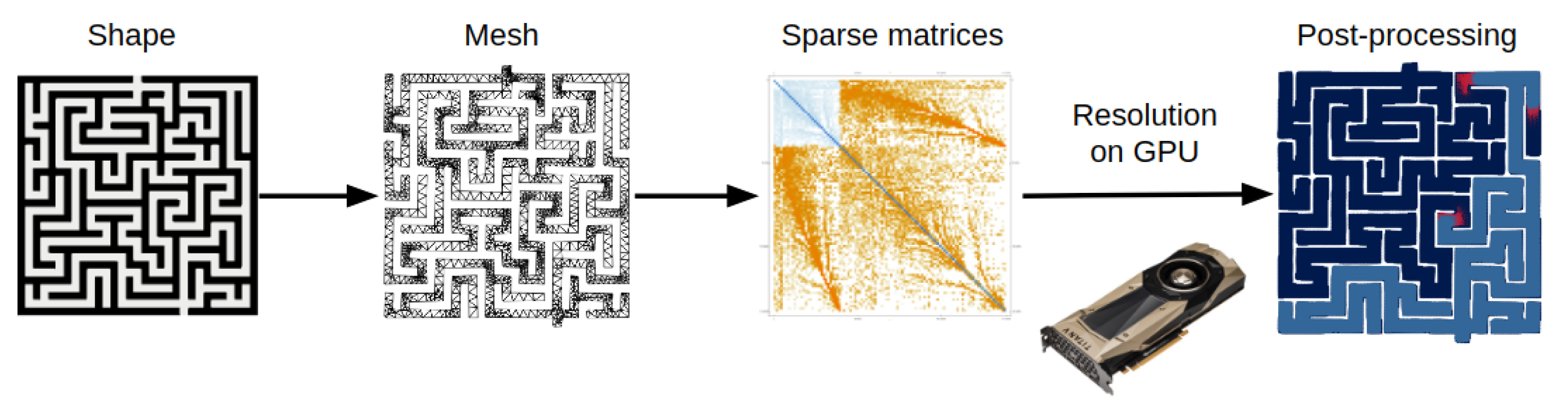
Here we solve reaction-diffusion equations in arbitrary geometries on GPUs with FEM [47,48,61]. This method discretizes in space and time a continuous PDE, formulating it as a problem of linear algebra for which the architecture of GPUs is uniquely appropriate. As a toy model, we study a nonlinear chemical system (a predator prey chemical oscillator) [27,28] in a tortuous geometry (a maze) [39]. This system was studied experimentally in a microfluidic device and captures the essence of how boundary conditions influence dynamics [39]. It generates traveling waves of preys that are closely followed by predators. The waves closely interact with the geometry of the maze: they propagate along the walls, split at junctions, and terminate at cul-de-sacs. Thus numerically solving this system with FEM is a challenging but informative case to study. The fixed geometries and the boundary conditions (no flux through the walls of the reactor) simplifies the FEM framework, while keeping a rich spatio-temporal dynamics. Moreover, the maze presents many sharp corners, which are known to be challenging for FEM, and represents a good testbed for porting the method to GPUs. A workflow of our methodology can be found in Figure 1.
2. Materials and Methods
2.1. Chemical System
We consider a biochemical predator prey systems as described by [27,28]. It consists of a prey species N, which is a DNA strand that replicates enzymatically, and which is predated by a predator strand P. This system mimics the dynamics of the Lotka-Voltera oscillator, and produces stable oscillations of concentration for days when run in a closed test tube.
The PDEs describing the dynamics of the system are
with Neumann boundary conditions (no flux through the wall of the reactor). The first term in the prey equation describe its auto-catalytic growth, the second terms describes its predation by the predator P. The laplacian term describe the diffusion of the prey. The first term in the predation equation describes the growth of the predator induced by the predation of the prey. We found that the null state was locally unstable, and that numerical error caused by the resolution would grow exponentially and cause the spontaneous generation of species. To regularize the equations, we added a small artificial term , which was chosen small enough so as not to affect the global dynamic of the system. To prevent negative concentrations caused by this term, we set concentrations to 0 when they become negative. The parameters for the simulations we present are: , and . The initial concentrations for the prey and the predator are taken to be 1 in the starting area (a small zone at the bottom of the maze) and 0 elsewhere.
2.2. Finite Element Method
We briefly present the Finite Element Method applied to our case [10]. We start from the reaction-diffusion PDE with Neumann boundary conditions (no flux through the boundaries of the reactor )
where and are the concentration of species N and P at position x and time t. The function encodes the local chemical reactions that produce or remove the species N and P. It is smooth, typically a polynomial function (in the case of mass action chemical kinetics) or rational function (in the case of enzymatic kinetics) of the concentrations of species.
We spatially discretize the reactor into a mesh. The mesh partitions the region into simple and non-overlapping geometrical cells (typically triangles), whose vertexes are called the nodes (Figure 1). Contrary to the fixed grid of the finite difference method, meshes allow for a flexible attribution of the computational budget. The physics of regions with an irregular geometry (e.g., turns in a maze) can be better fit by devoting more cells to their approximation. It must be noted that the problem of tessellating a geometric region into a mesh is an active topic of research, and will not be covered in this paper (we produce the mesh with Mathematica [69]). A mesh is associated with a basis of function , which is commonly defined to be 1 at the node i, and null on the other nodes. Again, there are many possible ways of defining how varies between nodes (piece-wise linear, piece-wise quadratic, …), and we use the basis of functions selected by the FEM software. Following the Galerkin method [70], we search for solution of Equation (Section 2.2) on the basis of functions
where and are the concentrations of species N and P at the node i and time t, and m is the number of nodes. Additionally we assume that the nodes are close to each other and that are sufficiently smooth, so that can be linearly interpolated between the nodes
We now expand Equation (Section 2.2) on the Galerkin basis
To derive the matrix differential equation, we define the element damping matrix D
and the element stiffness matrix S
The matrices D and S are sparse and positive-definite. They are mostly filled with 0 because and is 0 when the nodes i and j are not close to each other. Thanks to Green’s first identity and the Neumann boundary conditions
where is the boundary of and n the normal vector on this boundary. The integral over the boundary is null because of the Neumann conditions (no flux). We take the inner product on by multiplying Equation (Section 2.2) by and integrating over . We obtain the following matrix ordinary differential equation
where the function f is threaded on the vectors and .
This differential equation comprises two operators (the chemical reaction operator and the diffusion operator) with different physical properties. We integrate this equation using the split-operator method [71], splitting the reaction and diffusion operators and applying them alternatively to advance in time. More precisely, we discretize in time by defining and , where is a small time step and the integer k is the number of steps taken. At each time-step k, we first apply the chemical reaction operator (with Euler explicit method) to the vectors and , yielding intermediate vectors and
We then apply the diffusion operator with a time-step to the intermediate vectors and to obtain the vectors and at the step by solving the linear system
We chose the implicit Euler method for the diffusion step due to its better stability than the explicit version. We solve this linear equation with the conjugate gradient method (CGM) [72,73] because the matrix () is positive definite, and it only requires computing dot products and sparse matrices-vector products operations which are well adapted to GPUs.
By splitting the reaction and diffusion operators, we reduce the resolution of the PDE to operations that are well adapted to the parallel architectures of GPU. The reaction operator is a point-wise operator: it is already vectorized and easy to apply in a GPU. As for the diffusion operator, it reduces to linear algebra on sparse matrices and dense vectors, for which GPUs are highly performing.
2.3. Assembly of Stiffness and Damping Matrices
We used Mathematica [69] to assemble the stiffness and damping matrices. We started from a PNG image of a maze, which we binarized and converted into a geometrical region. We then discretized this region into a mesh with the FEM package of Mathematica, and assembled the corresponding damping and stiffness matrices. We controlled the size of the matrices (and the number of elements in the mesh) by changing the maximum allowed cell size during the discretization (smaller cells yield larger matrices). We then exported the matrices in CSV format.
2.4. Resolution of the Matrix Differential Equations
The bulk of the resolution was handled at a high level by a python program, which in turns called a C++ library accelerated using CUDA libraries (including CuBLAS [74] and CuSparse [75]) and home-made CUDA kernels to solve equation at a low level on the GPU. After parsing the damping and stiffness matrices from the CSV file, the python program loaded them onto the GPU.
For the diffusion operator, we solve the linear system with the conjugate gradient method (CGM) [72,73,76], as described in Algorithm 1. Each iteration of the CGM consists mostly of three operations: (1) products between a sparse matrix and a vector (which are handled by CuSparse [75]); (2) additions of two vectors (detailed in Algorithm 2); and (3) dot products between vectors. We implemented a version of the dot product that we optimized for GPUs, with increased performances compared to naive dot product algorithms (Algorithms 3 and 4). We iterate the solution until the relative error of the residual decreases below .
| Algorithm 1 User-level algorithm. |
|
| Algorithm 2 Addition of two vectors. |
|
| Algorithm 3 Naive dot product. |
|
| Algorithm 4 Optimized dot product. |
|
2.5. Comparison GPU and CPU
We compared the performances of the GPU and the CPU with the same algorithm (pointwise operation for the chemical reaction operator, and conjugate gradient method for the diffusion operator). We solved the system on GPU with a NVIDIA GPU Titan V (5120 CUDA cores, 12 GB memory, peak performance of TFLOPS for FP32 and and TFLOPS for FP64). We solved the system on CPU with a Intel Xeon Gold 6148 (20 Cores, 40 threads, base frequency Ghz) equipped with 188 GB ECC RAM. We estimated the power consumed by the GPU with the nvidia-smi command, and the power consumed by the CPU with the powerstat command (the power consumed by other electronic components such as the RAM or the disk is negligible). Simulations were performed in a Linux Mint 19.2 environment, with the CUDA library 10.2 and the NVIDIA driver 440.
2.6. Post-Processing
We plotted the time-lapses of the PDEs by drawing a rectangle at the location of each node in the mesh, the color of the rectangle indicating the local level prey and predators.
3. Results
3.1. Geometry
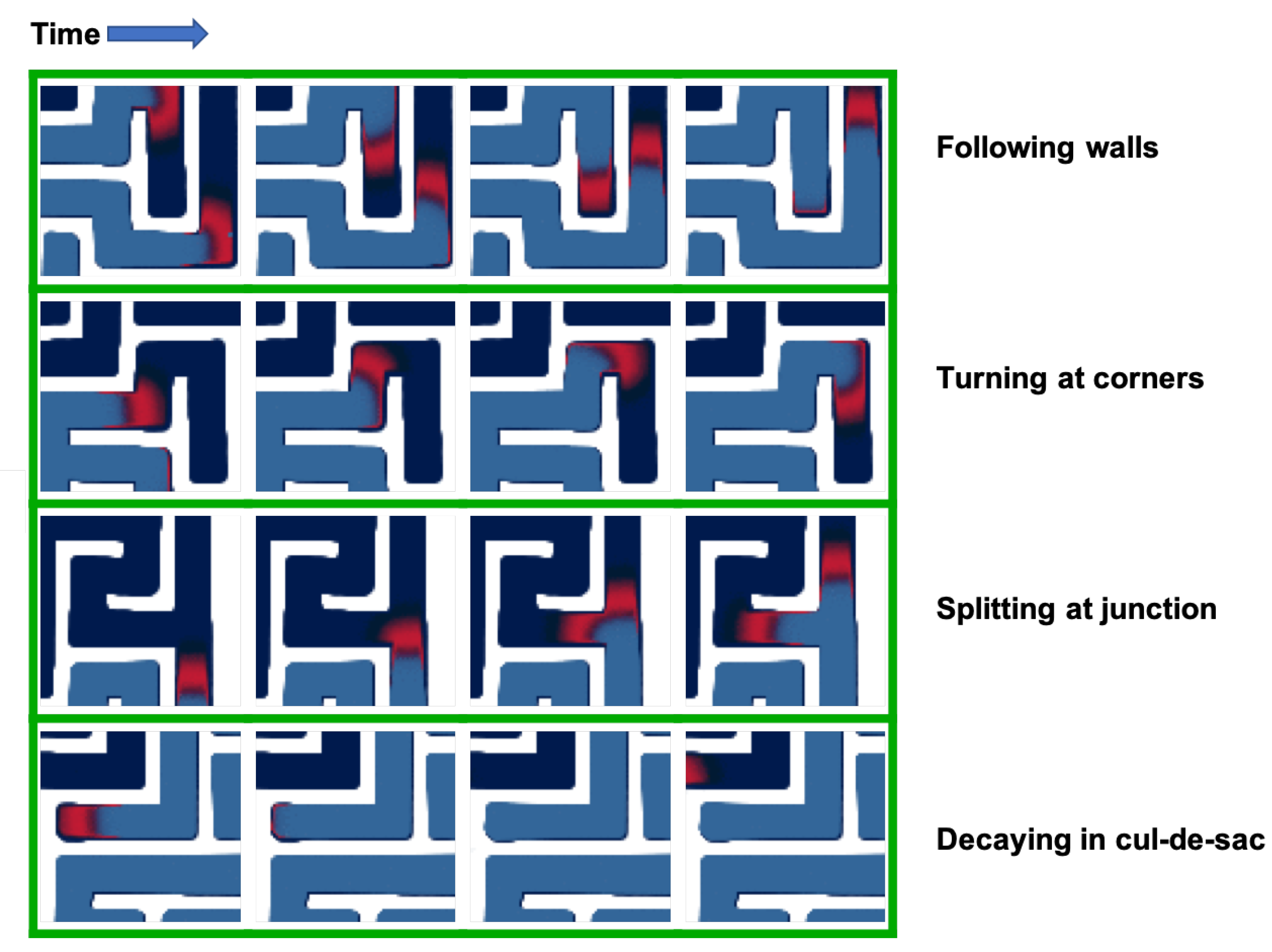
The simulations agree with experiments performed by other groups in microfluidics devices [39]. The system generates traveling waves of preys, closely followed by a massive front of predators (Figure 2). The waves propagate parallel to the walls of the maze, turn at corners and split at junctions into multiple waves that explore their own branch of the junction. The waves go extinct in cul-de-sacs, which can be explained by the unidirectional propagation of the waves: the preys get “cornered” and cannot escape from the predators.
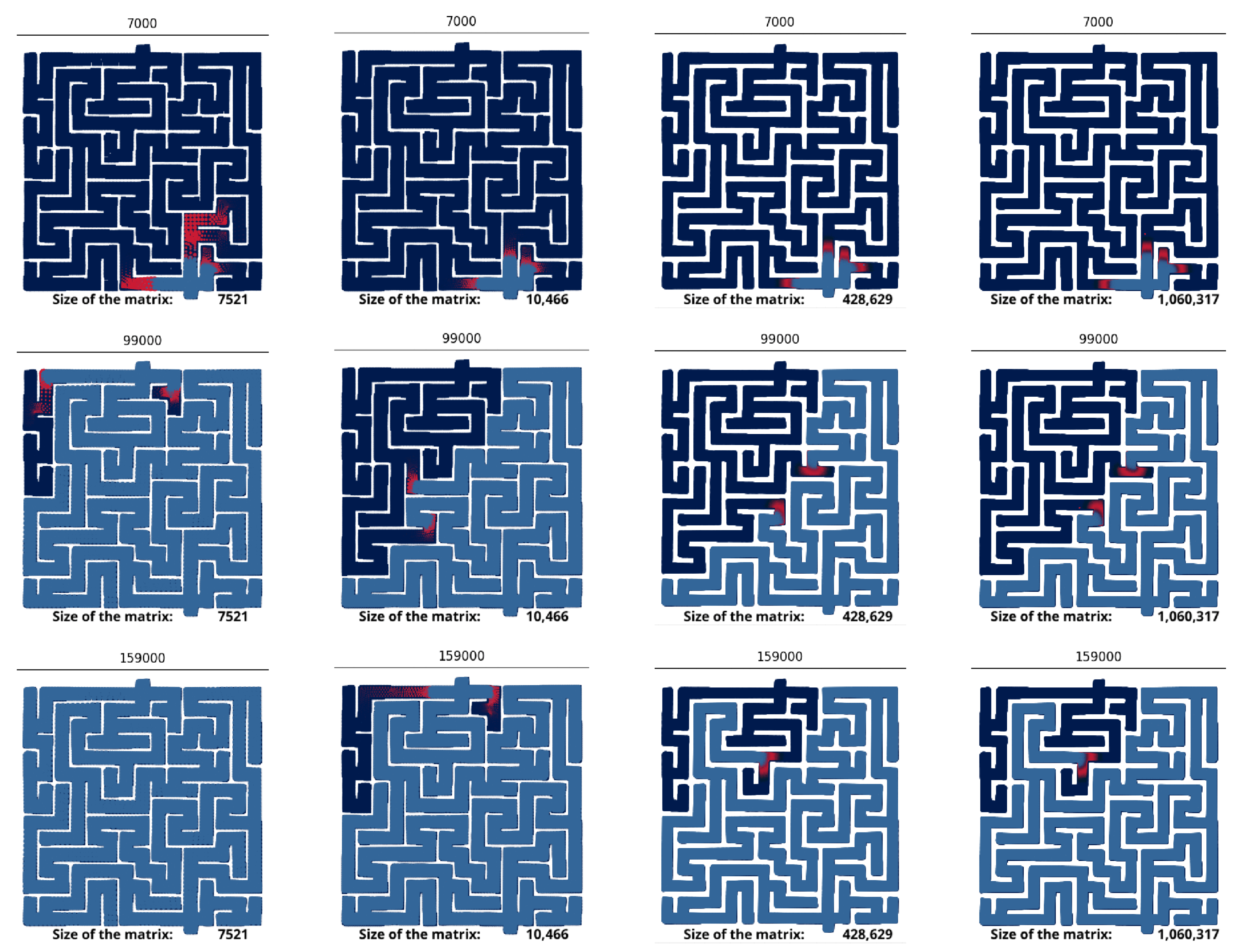
Our maze represents a challenging testbed for the FEM method, because it exhibits many sharp corners where it suddenly turns at a right angle. The normal vector to the wall is not smooth at these corners, which is known to induce difficulties for the FEM [49]. They are mitigated by finely graining the mesh near the sharp corners. Simulations confirm that the quality of the mesh is crucial to correctly solve the equations (Figure 3). Coarse meshes (∼7 k nodes) do not yield the same dynamic as fine meshes (∼1 M nodes). The prey is found to explore the maze much more quickly on small meshes, which suggests that coarse-graining produces numerical artifacts. We also observe the spontaneous appearance of preys far existing preys, which is not physically possible given the diffusive nature of the system: new chemical species can only appear close to existing ones.
3.2. Comparison Performance
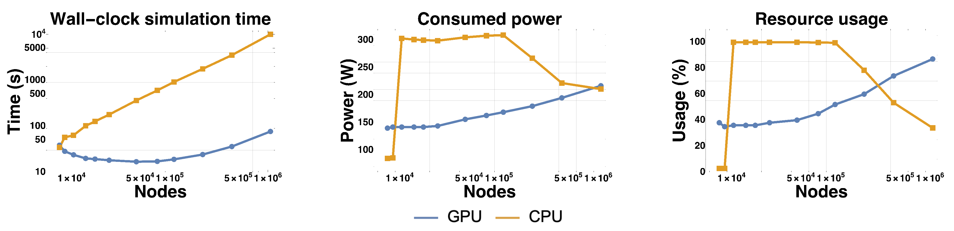
We studied the wall-clock time needed to simulate the system on CPU and GPU for 5000 steps (Figure 4). Overall the GPU is faster than the CPU, except for the smallest mesh size where the CPU is slightly faster. The speedup factor of the GPU over the CPU grows from ∼0.9 for the smallest mesh up to ∼130 for the largest mesh, where it plateaus. This speedup is over a multi-threaded implementation on a 20 cores (40 threads) CPU, which represents a substantial improvement over reported speedups for GPUs and FEM [51,57,77]. We attribute this speed up to an optimal use of the architecture of the GPU.
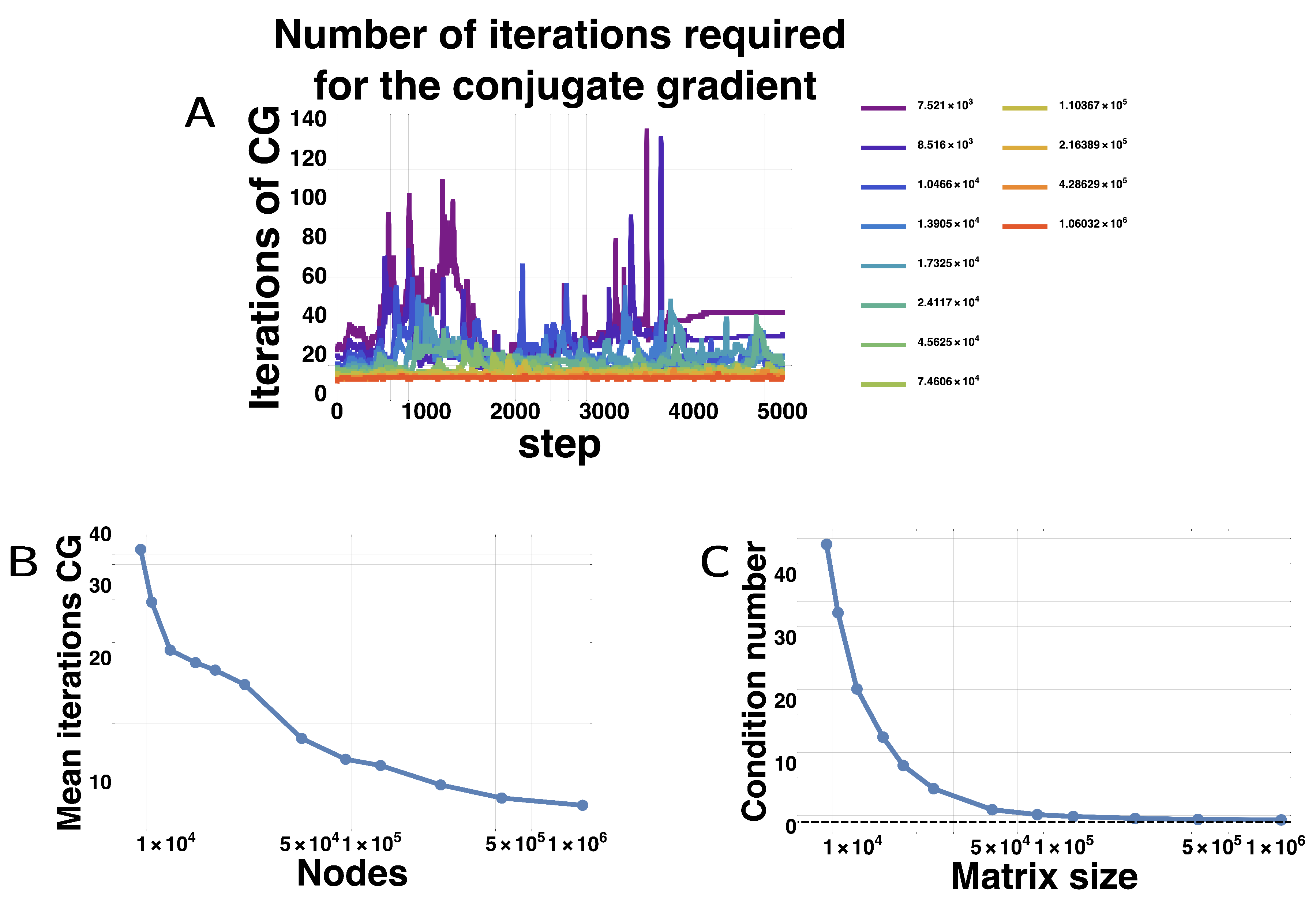
Surprisingly, the wall-clock time for simulation initially decreased with matrix size for the GPU. We found that the conjugate gradient method actually needed less and less iterations to arrive at the required precision as the matrices grew in size. Figure 5A shows for each matrix size, the number of iterations needed for the conjugate gradient method in function of the step number. For smaller matrices, the mean number of iterations is large and varies widely, but as the matrices get larger, the number of iterations becomes tamer and fewer. The mean number of iterations decreases with the matrix size (Figure 5B). We attribute this counter-intuitive behavior to the better conditioning of the matrices, which steadily decrease with finer meshes, almost reaching the minimum value of 1 (Figure 5C). We hypothesize that as the meshes become finer and finer, diffusion becomes more and more regular, locally resembling diffusion on a regular grid. More generally, sharp corners are better approximated by finer meshes, which likely helps in reducing the conditioning number [78,79].
We also profiled the power consumption and usage of GPU/CPU (Figure 4). The power consumption and usage of the GPU grew steadily and monotonously with matrix size. For the largest matrix, the power consumption was close to its theoretical maximum: ∼220 W for a thermal design power of 250 W. The largest matrices also come close to fully utilizing the computational power of the GPU, with an average usage ∼90%. This is remarkable, as it is often challenging to fully mobilize the parallel architecture of GPUs on a single real-world problem [4]. This trend was reverted for the CPU. The CPU usage decreased from 100% to ∼30% as the matrix size increased over ∼50,000 nodes, and the power consumption followed a similar trend. This pattern may be due to a switch from a compute-bound regime (where computation by the CPU is the bottleneck) to a memory-bound regime (where memory accesses to the matrices become the bottleneck). This under-usage of the CPU is in stark contrast with the almost complete usage of the GPU for large matrices, and clearly shows the superiority of the latter over the former for handling large problems in FEM.
3.3. Profiling
We profiled the time spent by the algorithm in each portion of the resolution. For the largest matrices, the reaction step only used 2% of the computation time, and 9% of the time was devoted to computing the matrix (), which is done only once at the beginning of the computation. Solving the linear system for the diffusion step with the conjugate gradient represents ∼90% of the total computation time. This diffusion step itself is broken down into taking the dot product of vectors (57% of the total time), summing vectors (18%) and initializing the vectors of the conjugate gradient (12%). Matrix multiplication only took 1% of the total computation time.
At first, it could seem counter-intuitive that much more time is spent on the dot product of vectors rather than the product of the matrix with vectors (which in itself is a collection of dot products between the rows of the matrix and the vector). However it must be remembered that the matrix is sparse, so that this dot product is done between a sparse vector and a dense vector, which requires only ∼a operations (where is the mean number of non-null elements per row in the matrix, and m the length of the multiplied vector). On the other side, taking the dot products of two dense vectors of length m is expected to require ∼m operations, and it cannot be fully parallelized, because intermediate dot products must be synchronized between the computing threads, which takes at least steps [80].
4. Discussion
We presented a framework for solving biochemical reaction-diffusion PDEs in arbitrary geometries with FEM on GPUs, which could benefit the DNA nanotechnology community to prototype and debug DNA-based reaction-diffusion systems [39,45,47]. The algorithm fully exploits the massive parallelism of GPUs, achieving a speedup of up to ∼130 over the same algorithm executed on a CPU. We identified a few bottlenecks to improve the future performances. Somewhat ironically, the processing of the PDEs with the GPU is so fast that pre-processing (initial parsing of the matrices) and post-processing (producing the time-lapse movie of the solution) become the bottleneck. Parsing large matrices from the CSV file only represents a few percent of the computation time of the CPU, but exceeds the computation time of the GPU. Storing the matrices directly in a float format would save the lengthy conversion from text to float. Alternatively, it would be beneficial to encode the matrices into a format optimized for vector architectures, such as the NVIDIA PKT format [80]. Moreover, post-processing operations are highly parallel, and in future implementations could be performed directly by the GPU, enabling real-time visualization of the solutions.
Additionally, more than half of the time was spent on computing dot products between dense vectors. Execution could potentially be accelerated with algorithms that use fewer dot products and rely almost exclusively on sparse matrix-vector products. Gradient descent is a candidate for this, though it does not enjoy the same speed of convergence as the conjugate gradient method for symmetric and positive-definite matrix. More simply, some dots products could be saved by reusing them between two successive iterations of the conjugate gradient, and the norm of the residual could be tested every other iteration.
Alternatively, it might be possible to increase the performance of the algorithm by applying different solvers, such as the conjugate gradient squared method or the Chebyshev iteration method [73]. However, these methods usually have an higher complexity per iterations compared to the baseline of the conjugate gradient, so these method would have to significantly reduce the number of iterations to be competitive.
Overall, this work shows that the massive parallelism of GPUs make them a powerful tool to speed up the simulation of PDEs and geometries used in DNA nanotechnology. We limited ourselves to reaction-diffusion PDEs, but similar equations, such as the advection-reaction-diffusion equation, could in principle be tackled (though the mathematical framework would be more involved because advection is a transport operator, which is hyperbolic) (See Supplementary Materials for details).
Supplementary Materials
The Github repository is available at https://github.com/cydouzo/ardis. A video of the exploration of the maze by the prey is available at https://www.youtube.com/watch?v=xzLqHQ3UFtM&list=LLEaa1Ya-FbKs8xfeaBesKFQ&index=2&t=0s.
Author Contributions
Conceptualization, N.A.-K. and A.J.G.; methodology, H.S., L.C., N.A.-K., and A.J.G.; software, H.S.; validation, H.S., L.C., N.A.-K. and A.J.G.; formal analysis, H.S. and A.J.G.; writing—original draft preparation, H.S., L.C., N.A.-K. and A.J.G.; supervision, L.C., T.F., M.H., N.A.-K., A.J.G.; funding acquisition, N.A.-K. and A.J.G. All authors have read and agreed to the published version of the manuscript.
Funding
This work was supported by a JSPS KAKENHI Grant Number JP19209045 to N.A.K., by a Grant-in-Aid for JSPS Fellows JP19F19722 to L.C., by a MEXT studentship to H.S., and by a GPU gift from NVIDIA to A.J.G.
Conflicts of Interest
The authors declare no conflict of interest. The funders had no role in the design of the study; in the collection, analyses, or interpretation of data; in the writing of the manuscript, or in the decision to publish the results.
References
- Brodtkorb, A.; Hagen, T.; Sætra, M. Graphics processing unit (GPU) programming strategies and trends in GPU computing. J. Parallel Distrib. Comput. 2013, 73, 4–13. [Google Scholar] [CrossRef] [Green Version]
- Ghorpade, J.; Parande, J.; Kulkarni, M.; Bawaskar, A. GPGPU processing in CUDA architecture. arXiv 2012, arXiv:1202.4347. [Google Scholar] [CrossRef]
- CUDA Performance Report. Available online: http://developer.download.nvidia.com/compute/cuda/6_5/rel/docs/CUDA_6.5_Performance_Report.pdf (accessed on 7 September 2020).
- Nickolls, J.; Buck, I.; Garland, M.; Skadron, K. Scalable parallel programming with CUDA. Queue 2008, 6, 40–53. [Google Scholar] [CrossRef] [Green Version]
- Abadi, M.; Barham, P.; Chen, J.; Chen, Z.; Davis, A.; Dean, J.; Devin, M.; Ghemawat, S.; Irving, G.; Isard, M.; et al. Tensorflow: A system for large-scale machine learning. In Proceedings of the 12th USENIX Symposium on Operating Systems Design and Implementation (OSDI 16), Savannah, GA, USA, 2–4 November 2016; pp. 265–283. [Google Scholar]
- Paszke, A.; Gross, S.; Chintala, S.; Chanan, G.; Yang, E.; DeVito, Z.; Lin, Z.; Desmaison, A.; Antiga, L.; Lerer, A. Automatic differentiation in pytorch. In Proceedings of the NIPS 2017 Workshop Autodiff, Long Beach, CA, USA, 9 December 2017. [Google Scholar]
- Rovigatti, L.; Šulc, P.; Reguly, I.; Romano, F. A comparison between parallelization approaches in molecular dynamics simulations on GPUs. J. Comput. Chem. 2015, 36, 1–8. [Google Scholar] [CrossRef] [PubMed] [Green Version]
- Glaser, J.; Nguyen, T.; Anderson, J.; Lui, P.; Spiga, F.; Millan, J.; Morse, D.; Glotzer, S. Strong scaling of general-purpose molecular dynamics simulations on GPUs. Comput. Phys. Commun. 2015, 192, 97–107. [Google Scholar] [CrossRef] [Green Version]
- Le Grand, S.; Götz, A.; Walker, R. SPFP: Speed without compromise—A mixed precision model for GPU accelerated molecular dynamics simulations. Comput. Phys. Commun. 2013, 184, 374–380. [Google Scholar] [CrossRef]
- Zienkiewicz, O.; Taylor, R.; Zhu, J. The Finite Element Method: Its Basis and Fundamentals; Elsevier: Amsterdam, The Netherlands, 2005. [Google Scholar]
- Fu, Z.; Lewis, T.; Kirby, R.; Whitaker, R. Architecting the finite element method pipeline for the GPU. J. Comput. Appl. Math. 2014, 257, 195–211. [Google Scholar] [CrossRef] [PubMed]
- Wu, W.; Heng, P.A. A hybrid condensed finite element model with GPU acceleration for interactive 3D soft tissue cutting. Comput. Animat. Virtual Worlds 2004, 15, 219–227. [Google Scholar] [CrossRef]
- Goddeke, D.; Buijssen, S.H.; Wobker, H.; Turek, S. GPU acceleration of an unmodified parallel finite element Navier-Stokes solver. In Proceedings of the 2009 International Conference on High Performance Computing & Simulation, Leipzig, Germany, 21–24 June 2009; pp. 12–21. [Google Scholar]
- Komatitsch, D.; Erlebacher, G.; Göddeke, D.; Michéa, D. High-order finite-element seismic wave propagation modeling with MPI on a large GPU cluster. J. Comput. Phys. 2010, 229, 7692–7714. [Google Scholar] [CrossRef]
- Joldes, G.R.; Wittek, A.; Miller, K. Real-time nonlinear finite element computations on GPU–Application to neurosurgical simulation. Comput. Methods Appl. Mech. Eng. 2010, 199, 3305–3314. [Google Scholar] [CrossRef] [Green Version]
- Dziekonski, A.; Sypek, P.; Lamecki, A.; Mrozowski, M. Finite element matrix generation on a GPU. Prog. Electromagn. Res. 2012, 128, 249–265. [Google Scholar] [CrossRef] [Green Version]
- Knepley, M.G.; Terrel, A.R. Finite element integration on GPUs. ACM Trans. Math. Softw. (TOMS) 2013, 39, 1–13. [Google Scholar] [CrossRef] [Green Version]
- Wang, S.; Wang, C.; Cai, Y.; Li, G. A novel parallel finite element procedure for nonlinear dynamic problems using GPU and mixed-precision algorithm. Eng. Comput. 2020, 37. [Google Scholar] [CrossRef]
- Huthwaite, P. Accelerated finite element elastodynamic simulations using the GPU. J. Comput. Phys. 2014, 257, 687–707. [Google Scholar] [CrossRef] [Green Version]
- Johnsen, S.F.; Taylor, Z.A.; Clarkson, M.J.; Hipwell, J.; Modat, M.; Eiben, B.; Han, L.; Hu, Y.; Mertzanidou, T.; Hawkes, D.J.; et al. NiftySim: A GPU-based nonlinear finite element package for simulation of soft tissue biomechanics. Int. J. Comput. Assist. Radiol. Surg. 2015, 10, 1077–1095. [Google Scholar] [CrossRef] [Green Version]
- Bauer, P.; Klement, V.; Oberhuber, T.; Žabka, V. Implementation of the Vanka-type multigrid solver for the finite element approximation of the Navier–Stokes equations on GPU. Comput. Phys. Commun. 2016, 200, 50–56. [Google Scholar] [CrossRef]
- Carrascal-Manzanares, C.; Imperiale, A.; Rougeron, G.; Bergeaud, V.; Lacassagne, L. A fast implementation of a spectral finite elements method on CPU and GPU applied to ultrasound propagation. Adv. Parallel Comput. 2018, 32, 339–348. [Google Scholar]
- Comsol, A. COMSOL Multiphysics User’s Guide; COMSOL: Stockholm, Sweden, 2005; Volume 10, p. 333. [Google Scholar]
- Soloveichik, D.; Seelig, G.; Winfree, E. DNA as a universal substrate for chemical kinetics. Proc. Natl. Acad. Sci. USA 2010, 107, 5393–5398. [Google Scholar] [CrossRef] [Green Version]
- Kim, J.; Winfree, E. Synthetic in vitro transcriptional oscillators. Mol. Syst. Biol. 2011, 7, 465. [Google Scholar] [CrossRef]
- Montagne, K.; Plasson, R.; Sakai, Y.; Fujii, T.; Rondelez, Y. Programming an in vitro DNA oscillator using a molecular networking strategy. Mol. Syst. Biol. 2011, 7, 466. [Google Scholar] [CrossRef]
- Fujii, T.; Rondelez, Y. Predator–prey molecular ecosystems. ACS Nano 2013, 7, 27–34. [Google Scholar] [CrossRef] [PubMed]
- Padirac, A.; Fujii, T.; Estévez-Torres, A.; Rondelez, Y. Spatial waves in synthetic biochemical networks. J. Am. Chem. Soc. 2013, 135, 14586–14592. [Google Scholar] [CrossRef]
- Srinivas, N.; Parkin, J.; Seelig, G.; Winfree, E.; Soloveichik, D. Enzyme-free nucleic acid dynamical systems. Science 2017, 358. [Google Scholar] [CrossRef] [PubMed] [Green Version]
- Genot, A.J.; Bath, J.; Turberfield, A.J. Reversible logic circuits made of DNA. J. Am. Chem. Soc. 2011, 133, 20080–20083. [Google Scholar] [CrossRef]
- Genot, A.J.; Bath, J.; Turberfield, A.J. Combinatorial displacement of DNA strands: Application to matrix multiplication and weighted sums. Angew. Chem. Int. Ed. 2013, 52, 1189–1192. [Google Scholar] [CrossRef] [PubMed]
- Stojanovic, M.N.; Stefanovic, D.; Rudchenko, S. Exercises in molecular computing. Acc. Chem. Res. 2014, 47, 1845–1852. [Google Scholar] [CrossRef]
- Lopez, R.; Wang, R.; Seelig, G. A molecular multi-gene classifier for disease diagnostics. Nat. Chem. 2018, 10, 746–754. [Google Scholar] [CrossRef]
- Cherry, K.M.; Qian, L. Scaling up molecular pattern recognition with DNA-based winner-take-all neural networks. Nature 2018, 559, 370–376. [Google Scholar] [CrossRef]
- Woods, D.; Doty, D.; Myhrvold, C.; Hui, J.; Zhou, F.; Yin, P.; Winfree, E. Diverse and robust molecular algorithms using reprogrammable DNA self-assembly. Nature 2019, 567, 366–372. [Google Scholar] [CrossRef] [Green Version]
- Song, T.; Eshra, A.; Shah, S.; Bui, H.; Fu, D.; Yang, M.; Mokhtar, R.; Reif, J. Fast and compact DNA logic circuits based on single-stranded gates using strand-displacing polymerase. Nat. Nanotechnol. 2019, 14, 1075–1081. [Google Scholar] [CrossRef]
- Chirieleison, S.M.; Allen, P.B.; Simpson, Z.B.; Ellington, A.D.; Chen, X. Pattern transformation with DNA circuits. Nat. Chem. 2013, 5, 1000. [Google Scholar] [CrossRef] [PubMed] [Green Version]
- Weitz, M.; Kim, J.; Kapsner, K.; Winfree, E.; Franco, E.; Simmel, F.C. Diversity in the dynamical behaviour of a compartmentalized programmable biochemical oscillator. Nat. Chem. 2014, 6, 295–302. [Google Scholar] [CrossRef] [PubMed] [Green Version]
- Zambrano, A.; Zadorin, A.; Rondelez, Y.; Estévez-Torres, A.; Galas, J. Pursuit-and-evasion reaction-diffusion waves in microreactors with tailored geometry. J. Phys. Chem. B 2015, 119, 5349–5355. [Google Scholar] [CrossRef] [PubMed]
- Genot, A.; Baccouche, A.; Sieskind, R.; Aubert-Kato, N.; Bredeche, N.; Bartolo, J.; Taly, V.; Fujii, T.; Rondelez, Y. High-resolution mapping of bifurcations in nonlinear biochemical circuits. Nat. Chem. 2016, 8, 760. [Google Scholar] [CrossRef] [PubMed]
- Baccouche, A.; Okumura, S.; Sieskind, R.; Henry, E.; Aubert-Kato, N.; Bredeche, N.; Bartolo, J.F.; Taly, V.; Rondelez, Y.; Fujii, T.; et al. Massively parallel and multiparameter titration of biochemical assays with droplet microfluidics. Nat. Protoc. 2017, 12, 1912–1932. [Google Scholar] [CrossRef] [PubMed]
- Kurylo, I.; Gines, G.; Rondelez, Y.; Coffinier, Y.; Vlandas, A. Spatiotemporal control of DNA-based chemical reaction network via electrochemical activation in microfluidics. Sci. Rep. 2018, 8, 6396. [Google Scholar] [CrossRef] [PubMed] [Green Version]
- Amodio, A.; Del Grosso, E.; Troina, A.; Placidi, E.; Ricci, F. Remote Electronic Control of DNA-Based Reactions and Nanostructure Assembly. Nano Lett. 2018, 18, 2918–2923. [Google Scholar] [CrossRef]
- Zadorin, A.S.; Rondelez, Y.; Galas, J.C.; Estevez-Torres, A. Synthesis of programmable reaction-diffusion fronts using DNA catalyzers. Phys. Rev. Lett. 2015, 114, 068301. [Google Scholar] [CrossRef]
- Scalise, D.; Schulman, R. Emulating cellular automata in chemical reaction–diffusion networks. Nat. Comput. 2016, 15, 197–214. [Google Scholar] [CrossRef]
- Zadorin, A.S.; Rondelez, Y.; Gines, G.; Dilhas, V.; Urtel, G.; Zambrano, A.; Galas, J.C.; Estévez-Torres, A. Synthesis and materialization of a reaction–diffusion French flag pattern. Nat. Chem. 2017, 9, 990. [Google Scholar] [CrossRef] [Green Version]
- Abe, K.; Kawamata, I.; Shin-ichiro, M.; Murata, S. Programmable reactions and diffusion using DNA for pattern formation in hydrogel medium. Mol. Syst. Des. Eng. 2019, 4, 639–643. [Google Scholar] [CrossRef]
- Chen, S.; Seelig, G. Programmable patterns in a DNA-based reaction–diffusion system. Soft Matter 2020, 16, 3555–3563. [Google Scholar] [CrossRef] [PubMed] [Green Version]
- Bardi, I.; Biro, O.; Dyczij-Edlinger, R.; Preis, K.; Richter, K.R. On the treatment of sharp corners in the FEM analysis of high frequency problems. IEEE Trans. Magn. 1994, 30, 3108–3111. [Google Scholar] [CrossRef]
- Molnár, F., Jr.; Izsák, F.; Mészáros, R.; Lagzi, I. Simulation of reaction–diffusion processes in three dimensions using CUDA. Chemom. Intell. Lab. Syst. 2011, 108, 76–85. [Google Scholar] [CrossRef] [Green Version]
- Descombes, S.; Dhillon, D.; Zwicker, M. Optimized CUDA-based PDE Solver for Reaction Diffusion Systems on Arbitrary Surfaces. In International Conference on Parallel Processing and Applied Mathematics; Springer: Berlin/Heidelberg, Germany, 2015; pp. 526–536. [Google Scholar]
- Sanderson, A.R.; Meyer, M.D.; Kirby, R.M.; Johnson, C.R. A framework for exploring numerical solutions of advection–reaction–diffusion equations using a GPU-based approach. Comput. Vis. Sci. 2009, 12, 155–170. [Google Scholar] [CrossRef]
- Sato, D.; Xie, Y.; Weiss, J.N.; Qu, Z.; Garfinkel, A.; Sanderson, A.R. Acceleration of cardiac tissue simulation with graphic processing units. Med. Biol. Eng. Comput. 2009, 47, 1011–1015. [Google Scholar] [CrossRef] [Green Version]
- Mena, A.; Ferrero, J.M.; Matas, J.F.R. GPU accelerated solver for nonlinear reaction–diffusion systems. Application to the electrophysiology problem. Comput. Phys. Commun. 2015, 196, 280–289. [Google Scholar] [CrossRef]
- Sjodin, B. What’s the Difference between FEM, FDM, and FVM. Mach. Des. 2016. Available online: https://www.machinedesign.com/3d-printing-cad/fea-and-simulation/article/21832072/whats-the-difference-between-fem-fdm-and-fvm (accessed on 7 September 2020).
- Pera, D.; Málaga, C.; Simeoni, C.; Plaza, R. On the efficient numerical simulation of heterogeneous anisotropic diffusion models for tumor invasion using GPUs. Rend. Mat. E Sue Appl. 2019, 40, 233–255. [Google Scholar]
- Gormantara, A.; Pranowo, P. Parallel simulation of pattern formation in a reaction-diffusion system of FitzHugh-Nagumo using GPU CUDA. In AIP Conference Proceedings; AIP Publishing LLC: College Park, MD, USA, 2020; Volume 2217, p. 030134. [Google Scholar]
- Zaikin, A.; Zhabotinsky, A. Concentration wave propagation in two-dimensional liquid-phase self-oscillating system. Nature 1970, 225, 535–537. [Google Scholar] [CrossRef]
- Turing, A.M. The chemical basis of morphogenesis. Bull. Math. Biol. 1990, 52, 153–197. [Google Scholar] [CrossRef]
- Dalchau, N.; Seelig, G.; Phillips, A. Computational design of reaction-diffusion patterns using DNA-based chemical reaction networks. In International Workshop on DNA-Based Computers; Springer: Berlin/Heidelberg, Germany, 2014; pp. 84–99. [Google Scholar]
- Zenk, J.; Scalise, D.; Wang, K.; Dorsey, P.; Fern, J.; Cruz, A.; Schulman, R. Stable DNA-based reaction–diffusion patterns. RSC Adv. 2017, 7, 18032–18040. [Google Scholar] [CrossRef] [Green Version]
- Smith, S.; Dalchau, N. Beyond activator-inhibitor networks: The generalised Turing mechanism. arXiv 2018, arXiv:1803.07886. [Google Scholar]
- Smith, S.; Dalchau, N. Model reduction enables Turing instability analysis of large reaction–diffusion models. J. R. Soc. Interface 2018, 15, 20170805. [Google Scholar] [CrossRef] [Green Version]
- Joesaar, A.; Yang, S.; Bögels, B.; van der Linden, A.; Pieters, P.; Kumar, B.P.; Dalchau, N.; Phillips, A.; Mann, S.; de Greef, T.F. DNA-based communication in populations of synthetic protocells. Nat. Nanotechnol. 2019, 14, 369–378. [Google Scholar] [CrossRef]
- Urtel, G.; Estevez-Torres, A.; Galas, J.C. DNA-based long-lived reaction–diffusion patterning in a host hydrogel. Soft Matter 2019, 15, 9343–9351. [Google Scholar] [CrossRef]
- Gines, G.; Zadorin, A.; Galas, J.C.; Fujii, T.; Estevez-Torres, A.; Rondelez, Y. Microscopic agents programmed by DNA circuits. Nat. Nanotechnol. 2017, 12, 351–359. [Google Scholar] [CrossRef]
- Dupin, A.; Simmel, F.C. Signalling and differentiation in emulsion-based multi-compartmentalized in vitro gene circuits. Nat. Chem. 2019, 11, 32–39. [Google Scholar] [CrossRef]
- Kasahara, Y.; Sato, Y.; Masukawa, M.K.; Okuda, Y.; Takinoue, M. Photolithographic shape control of DNA hydrogels by photo-activated self-assembly of DNA nanostructures. APL Bioeng. 2020, 4, 016109. [Google Scholar] [CrossRef]
- Wolfram Research, Inc. Mathematica, Version 12.1; Wolfram Research, Inc.: Champaign, IL, USA, 2020. [Google Scholar]
- Galerkin, B. Series occurring in various questions concerning the elastic equilibrium of rods and plates. Eng. Bull. (Vestn. Inzhenerov) 1915, 19, 897–908. [Google Scholar]
- Strang, G. On the construction and comparison of difference schemes. SIAM J. Numer. Anal. 1968, 5, 506–517. [Google Scholar] [CrossRef]
- Ahamed, A.; Magoules, F. Conjugate gradient method with graphics processing unit acceleration: CUDA vs. OpenCL. Adv. Eng. Softw. 2017, 111, 32–42. [Google Scholar] [CrossRef]
- Barrett, R.; Berry, M.; Chan, T.; Demmel, J.; Donato, J.; Dongarra, J.; Eijkhout, V.; Pozo, R.; Romine, C.; Van der Vorst, H. Templates for the Solution of Linear Systems: Building Blocks for Iterative Methods; SIAM: Philadelphia, PA, USA, 1994. [Google Scholar]
- Nvidia, C. Cublas Library; NVIDIA Corp.: Santa Clara, CA, USA, 2008; Volume 15, p. 31. [Google Scholar]
- Naumov, M.; Chien, L.; Vandermersch, P.; Kapasi, U. CUSPARSE library: A set of basic linear algebra subroutines for sparse matrices. In Proceedings of the GPU Technology Conference, San Jose, CA, USA, 20–23 September 2010; Volume 2070. [Google Scholar]
- Hestenes, M.; Stiefel, E. Methods of conjugate gradients for solving linear systems. J. Res. Natl. Bur. Stand. 1952, 49, 409–436. [Google Scholar] [CrossRef]
- Hutton, T.; Munafo, R.; Trevorrow, A.; Rokicki, T.; Wills, D. Ready, A Cross-Platform Implementation of Various Reaction-Diffusion Systems. 2015. Available online: https://github.com/GollyGang/ready (accessed on 7 September 2020).
- Du, Q.; Wang, D.; Zhu, L. On mesh geometry and stiffness matrix conditioning for general finite element spaces. SIAM J. Numer. Anal. 2009, 47, 1421–1444. [Google Scholar] [CrossRef] [Green Version]
- Ramage, A.; Wathen, A. On preconditioning for finite element equations on irregular grids. SIAM J. Matrix Anal. Appl. 1994, 15, 909–921. [Google Scholar] [CrossRef]
- Bell, N.; Garland, M. Efficient Sparse Matrix-Vector Multiplication on CUDA; Technical Report, Nvidia Technical Report NVR-2008-004; Nvidia Corporation: Santa Clara, CA, USA, 2008. [Google Scholar]
Figure 1.
Workflow of our methodology. We start from a bitmap image of a maze that is discretized into a mesh with a FEM software, which then assembles the stiffness and damping matrices. We solve the matrix ordinary differential equations on the GPU, and then plot the results with the CPU.
Figure 1.
Workflow of our methodology. We start from a bitmap image of a maze that is discretized into a mesh with a FEM software, which then assembles the stiffness and damping matrices. We solve the matrix ordinary differential equations on the GPU, and then plot the results with the CPU.

Figure 2.
Effect of boundary conditions on the dynamic of the system. The predator-prey system generates traveling waves of preys (in red) followed by a front of predators (blue). The traveling waves closely interact with the geometry of the reactor. They follow straight walls, turn at corners, split at junction, and go extinct in cul-de-sacs. For each geometrical effect, four representative snapshots are presented (taken at an interval of 2000 time-steps).

Figure 3.
Numerical artifacts for coarse grained meshes. Snapshot of the simulations for coarse and fine meshes. The time-step is indicated at the top of each snapshot. The size of the mesh is indicated at the bottom of the snapshots. The prey is colored in red, and the predator colored in blue.
Figure 3.
Numerical artifacts for coarse grained meshes. Snapshot of the simulations for coarse and fine meshes. The time-step is indicated at the top of each snapshot. The size of the mesh is indicated at the bottom of the snapshots. The prey is colored in red, and the predator colored in blue.

Figure 4.
Comparison of performances of the GPU and the CPU for 5000 steps. The plots compare resolution on the GPU and on the CPU for 3 metrics of interests: wall-clock simulation time, average power consumption and resource usage.
Figure 4.
Comparison of performances of the GPU and the CPU for 5000 steps. The plots compare resolution on the GPU and on the CPU for 3 metrics of interests: wall-clock simulation time, average power consumption and resource usage.

Figure 5.
Numerical difficulty of the Conjugate Gradient Method. (A) Number of iterations required by the CGM to reach convergence (relative error of the residual decreases below ) for different matrix sizes; (B) Mean number of iterations of the CGM extracted from (A); (C) condition number of the matrix ) according to the matrix size. The dashed line shows the value of 1, which is the absolute minimum for a condition number. The condition number of the matrix was taken by multiplying the norm of the matrix and its inverse, each estimated on random vectors of norm 1.


Table 1.
Examples of representative works on GPU-accelerated resolutions of reaction-diffusion PDEs. These methods include Finite Difference Methods (FDM) and Finite Element Methods (FEM) [55]. For each study, we present a typical speed-up between CPU and GPU implementations.
Table 1.
Examples of representative works on GPU-accelerated resolutions of reaction-diffusion PDEs. These methods include Finite Difference Methods (FDM) and Finite Element Methods (FEM) [55]. For each study, we present a typical speed-up between CPU and GPU implementations.
| Paper | Method | Problem | Speedup (CPU vs. GPU) |
|---|---|---|---|
| Sanderson et al., 2009 [52] | FDM | grid mesh, Advection-Reaction-Diffusion | ∼5–10x vs. one CPU core |
| Molnar et al., 2011 [50] | FDM | grid mesh, Turing Patterns, Cahn–Hilliard eq., … | ∼5–40x vs. one CPU thread |
| Pera et al., 2019 [56] | FDM | grid mesh, tumor growth | ∼100–500x vs. 8-core CPU |
| Gormantara et al., 2020 [57] | FDM | grid mesh, FitzHugh-Nahumo model | ∼10x vs. CPU |
| Sato et al., 2009 [53] | FEM+ODE | 3D cardiac simulations | ∼0.6x vs. 32-CPU cluster |
| Mena et al., 2015 [54] | FEM+ODE | 3D cardiac simulations | ∼50x vs. one CPU core |
| Descombes et al., 2015 [51] | FEM | chemotactic reaction-diffusion on arbitrary surface | ∼100–300x vs. 4-core CPU |
© 2020 by the authors. Licensee MDPI, Basel, Switzerland. This article is an open access article distributed under the terms and conditions of the Creative Commons Attribution (CC BY) license (http://creativecommons.org/licenses/by/4.0/).
Share and Cite
MDPI and ACS Style
Sellami, H.; Cazenille, L.; Fujii, T.; Hagiya, M.; Aubert-Kato, N.; Genot, A.J. Accelerating the Finite-Element Method for Reaction-Diffusion Simulations on GPUs with CUDA. Micromachines 2020, 11, 881. https://doi.org/10.3390/mi11090881
AMA Style
Sellami H, Cazenille L, Fujii T, Hagiya M, Aubert-Kato N, Genot AJ. Accelerating the Finite-Element Method for Reaction-Diffusion Simulations on GPUs with CUDA. Micromachines. 2020; 11(9):881. https://doi.org/10.3390/mi11090881
Chicago/Turabian StyleSellami, Hedi, Leo Cazenille, Teruo Fujii, Masami Hagiya, Nathanael Aubert-Kato, and Anthony J. Genot. 2020. "Accelerating the Finite-Element Method for Reaction-Diffusion Simulations on GPUs with CUDA" Micromachines 11, no. 9: 881. https://doi.org/10.3390/mi11090881
Note that from the first issue of 2016, this journal uses article numbers instead of page numbers. See further details here.