Article

Assessing 3-D Spatial Extent of Near-Road Air Pollution around a Signalized Intersection Using Drone Monitoring and WRF-CFD Modeling

1
Department of Environmental Science, Kangwon National University, Chuncheon 24341, Korea
2
School of Natural Resources and Environmental Science, Kangwon National University, Chuncheon 24341, Korea
*
Author to whom correspondence should be addressed.
Int. J. Environ. Res. Public Health 2020, 17(18), 6915; https://doi.org/10.3390/ijerph17186915
Submission received: 28 July 2020 / Revised: 17 September 2020 / Accepted: 19 September 2020 / Published: 22 September 2020
(This article belongs to the Special Issue Spatial Modeling of Air Pollutant Variability)

Abstract

:
In this study, we have assessed the three-dimensional (3-D) spatial extent of near-road air pollution around a signalized intersection in a densely populated area using collaborating methodologies of stationary measurements, drone monitoring, and atmospheric dispersion modeling. Stationary measurement data collected in the roadside apartment building showed a substantial effect of emitted pollutants, such as nitrogen oxides (NOx), black carbon (BC), and ultrafine particles (UFPs), especially during the morning rush hours. Vertical drone monitoring near the road intersection exhibited a steeper decreasing trend with increasing altitude for BC concentration rather than for fine particulate matter (PM2.5) concentration below the apartment building height. Atmospheric NOx dispersion was simulated using the weather research and forecasting (WRF) and computational fluid dynamics (CFD) models for the drone measurement periods. Based on the agreement between the measured BC and simulated NOx concentrations, we concluded that the air pollution around the road intersection has adverse effects on the health of residents living within the 3-D spatial extent within at least 120 m horizontally and a half of building height vertically during the morning rush hours. The comparability between drone monitoring and WRF-CFD modeling can further guarantee the identification of air pollution hotspots using the methods.

Graphical Abstract

1. Introduction

The urban proportion of the global population is 55% and is expected to increase to 68% by 2050 [1]. Owing to the high population densities in urban areas, public use facilities, such as schools and parks in residential areas, have become closer to roads with increasing traffic. As a result, residents’ exposure to harmful air pollutants emitted by on-road mobile sources has become a serious health and environmental problem [2,3]. Air pollutants emitted from vehicles, such as nitrogen oxides (NOx), carbon monoxide (CO), black carbon (BC), and ultrafine particles (UFPs) with a diameter less than 100 nm, have caused various environmental diseases such as respiratory diseases, stunted growth in children, and cardiovascular diseases [4,5].
Environmental diseases caused by air pollutants are more likely to occur in air pollution hotspots where there are many pedestrians and mobile sources intensively [6,7]. Signalized road intersections are representative hotspots of air pollution in urban areas. Because frequent stops, accelerations, and decelerations of vehicles at traffic signals occur around busy intersections, signalized road intersections have a high risk of exposure to air pollutants emitted by vehicles, with more than 20% exceeding the average CO and NOx emissions compared to roundabouts [8,9,10]. In addition, high-rise buildings near signalized intersections can weaken air flow and then worsen air quality [11,12].
Traffic-related air pollutants such as NOx and UFPs can be reduced as the distance from the intersection increases by up to a few hundred meters in an open space [13], complex urban areas [14,15], and urban parks [16]. The horizontal gradient of pollutant concentration with increasing distance from the road is determined by road geometries and atmospheric environment such as wind speed and direction with respect to the road axis as well as on-road pollutant emissions [17]. A few previous studies conducted measurements on roadside high-rise buildings to investigate the vertical concentration profiles of traffic-related air pollutants. Major pollutants such as PM10, PM2.5(particulate matter with a diameter less than 10 μm and 2.5 μm, respectively) NO2, CO2, and CO emitted from the adjacent roads were gradually reduced as the measurement height increased because of vertical mixing [18,19]. To overcome the spatial limitations of vertical distribution measurements based on fixed structures such as towers and buildings, mobile measurements using a drone have recently been attempted by many researchers. A previous study [20] measured the vertical distribution of a particle number concentration using a drone near a highway in Australia and observed near-road air pollution up to at an approximately 40 m altitude. In addition, another previous study [21] measured the vertical PM2.5 distributions in the middle of roads using a drone, and found that these concentrations remained constant within a 35 m altitude and began to decrease above the altitude because of the effect of roadside trees.
Although air pollutant concentrations near hotspots such as road intersections show high spatiotemporal variabilities, simultaneous measurement of these concentrations at fixed locations to demonstrate the three-dimensional (3-D) spatial distribution is extremely challenging, especially in urban areas. To solve this problem, a computational fluid dynamics (CFD) model that simulates the airflow and pollutant distribution at road and building scales has been utilized [22,23,24]. The 3-D spatial distribution of near-road air pollution around hotspots is likely to be derived by the airflow around buildings, such as recirculating flows between roadside buildings and channeling flows inside building arrangements [25,26,27]. The peak concentration locations in a street canyon between buildings were substantially different within a 30 m altitude from the ground depending on the building geometries (i.e., height and symmetry) on both sides [28].
To provide realistic meteorological inputs for the inflow boundary conditions of the CFD model, the weather research and forecasting (WRF) model coupled to the CFD model is one of the several reliable methodologies [29]. A WRF-CFD modeling study [30] confirmed that the simulation accuracy of simulation results using the coupled WRF-CFD model improved compared to that of simulation results using the CFD model only. The high spatiotemporal resolution of meteorological input data, such as 3-D air temperature, wind components, and turbulent kinetic energy fields, with an approximately 1 km resolution is the essential merit of the coupled WRF-CFD model [31]. The coupled WRF-CFD modeling approach provides accurate meteorological inputs from a mesoscale model in simulating realistic urban air quality at a high resolution [32].
On-site measurement and high-resolution numerical simulations are complementary methods used to identify the spatiotemporal variation near air pollution hotspots in urban areas. Although a high-resolution numerical simulation is beneficial for providing detailed identification of spatiotemporal variability, an on-site measurement is essential for verifying and improving the reliability of numerical simulation results. However, it is still challenging to find the comparability between the smoothed concentration fields simulated using a numerical model and the instantaneous concentration fields measured by a mobile monitoring instrument. In this study, we use collaborating methodologies of stationary and mobile monitoring together with the coupled WRF-CFD modeling to quantitatively assess the 3-D spatial extent of near-road air pollution near an intersection in an urban residential area. Section 2 provides the methodology, Section 3 presents and discusses the results, and Section 4 concludes this paper.

2. Methods

2.1. Study Site and Period

The site of interest is a signalized intersection in a residential area in Chuncheon, Gangwon Province in the Republic of Korea (37.88° N, 127.73° E, 105 m a.s.l. (i.e., above sea level)). Chuncheon is a medium-sized city located in an inland basin near a large river, with a population of approximately 280,000. Toegye Intersection surrounded by several apartment complex of 18 floors or less is the signalized intersection where six-lane roads in three directions intersect with a four-lane road in one direction. Because it is located on the road entering from the city center to the highway, the intersection is busy, containing significant traffic that consists of express buses and heavy-duty vehicles as well as passenger cars. An urban park is located at the northern side of the intersection, and a small stream running from south to north crosses the urban park (Figure 1).
The two periods of interest were on four consecutive weekdays from 12 to 15 March 2019 (P1) and on five consecutive weekdays from 1 to 5 April 2019 (P2). The drone measurements were conducted in the urban park at approximately 50 m north of the center of the intersection. The stationary measurements were conducted on the 11th floor (i.e., 30 m altitude above the ground) of an apartment building at approximately 150 m northwest of the center of the intersection. Two measurement locations were placed at the downwind side of the intersection when a southerly wind prevailed. From 10 min before every drone measurement, we recorded traffic videos of the intersection for two cycles of traffic signals (i.e., 320 s). Then, the traffic volumes were manually counted from the recorded video. Chuncheon automatic weather station (AWS), approximately 5 km North of the Toegye Intersection, is chosen for background meteorological observation data. In addition, AWS instruments were additionally installed on the sidewalk to the south of the Toegye Intersection for roadside meteorological observation data, such as temperature, relative humidity, wind direction, and wind speed. The air quality monitoring station (AQMS) data were obtained for urban background concentrations of air pollutants (i.e., PM2.5, NO2, O3).

2.2. Drone and Stationary Measurements

The drone measurements were performed during the morning rush hours (8–9 a.m.) on selected three days of 12, 14, and 15 March 2019 (P1D), and on another selected three days of 1, 2, and 3 April 2019 (P2D). The drone used in this study was an octocopter drone (DJI A2) with rotary wings that can hover at a certain altitude. The total width and height are 105 and 50 cm, respectively, and the flight time is approximately 10 min with a carrying capacity of 2 kg or more [33]. Meteorological (Imet-XQ2 for air temperature (Temp) and relative humidity (RH)), particulate matter (AM520 for PM2.5 and MA200 for BC), and gaseous (Aeroqual 500 for O3) sensors were used for drone measurements. These are small instruments that do not exceed 620 g per device (Table 1). The inlets connected to AM520 and MA200 to measure PM2.5 and BC were installed approximately 20 cm above the main body of drone to minimize the effect of turbulence from the propellers of the drone as suggested by a previous study [34]. The drone was operated in 30-min intervals at 8:00, 8:30, and 9:00 a.m. with a 40-s hovering at every altitude (i.e., 0, 10, 20, 30, 40, 50, 70, and 100 m) for the P1D and P2D periods. During the hovering time at each altitude, the first 20 s was regarded as an initial stabilization, and the measurement data for the following 20 s was averaged and used in the analysis.
The instruments used for stationary measurements were an optical particle counter (OPC) (Grimm Model 1.109A) for PM10, PM2.5, and PM1, mini aethalometer (Aethlab MA200) for BC, scanning mobility particle sizer (SMPS) (TSI SMPS3910) for nano-size particles, NO/NO2/NOx analyzer (Eco Physics nCLD AL) for NOx, and CO2/O3 analyzer (KINSCO technology) for CO2 and O3 (Table 1). The inlet of every measuring instrument was installed outside approximately 1 m away from the apartment building wall to measure the outdoor air. Because the OPC only measures atmospheric particles with a diameter larger than 0.25 μm, the PM2.5 mass concentration was calculated by adding the mass concentration of smaller particles with a diameter between 11.5 and 205.4 nm measured by SMPS to the PM2.5 concentration measured by OPC. The PM2.5 concentration measured by AM520 used in the drone measurement tends to be higher than the PM2.5 concentration measured by OPC. Hence, the overestimated PM2.5 concentration measured by AM520 was fitted to the PM2.5 concentration measured by OPC at the same altitude.

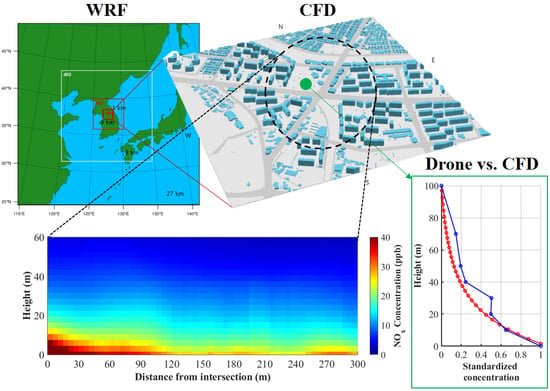
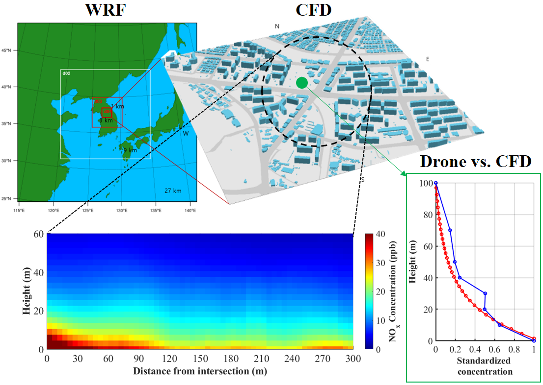
2.3. WRF-CFD Modeling

The coupled WRF-CFD model processes initial and boundary input data of the CFD model from the mesoscale meteorological fields (e.g., air temperature, wind direction, and wind speed) simulated by the WRF model [31]. The WRF model version 3.9.1 used in this study is a mesoscale meteorological model developed by the NCAR/UCAR (National Center for Atmospheric Research/University Corporation for Atmospheric Research, CO, USA). The simulation domain covers Northeast Asia and is centered at Chuncheon, Republic of Korea (37.85° N, 127.73° E). Four nested domains with horizontal grid sizes of 27, 9, 3, and 1 km were used (Figure 2a). The simulation periods were from 12 UTC on 10 to 12 March UTC on 15 March 2019 (P1) and from 00 UTC on 31 March 2019 to 00 UTC on 6 April 2019 (P2). The spin-up times were 35 and 23 h for P1 and P2, respectively. For the initial and boundary conditions, we used the National Centers for Environmental Prediction (NCEP) FNL reanalysis data with a 6 h interval and a horizontal resolution of 1° × 1°, the sea surface temperature data with a 24 h interval and a horizontal resolution of 0.5° × 0.5° archived by the National Oceanic and Atmospheric Administration (NOAA), and the United States Geological Survey (USGS) land cover data with a 1 km resolution. The planetary boundary layer (PBL) parametrization process greatly affects the accuracy of the near-surface air temperature and wind simulations. The Yonsei University (YSU) PBL scheme is a non-local PBL parameterization scheme that calculates the PBL height using the bulk Richardson number [35]. By contrast, the Mellor-Yamada-Janjic (MYJ) PBL scheme is a local PBL parameterization scheme that determines the vertical mixing through the calculation of turbulent kinetic energy (TKE), and thus calculates the PBL height from the TKE profile [36]. Therefore, the MYJ and YSU schemes were selected for simulation periods of P1 and P2, respectively, after examining the accuracy of the simulation results.
The CFD model is a Reynolds-averaged Navier–Stokes equations (RANS) model with a renormalization group (RNG) kε turbulent closure scheme, which simulates the atmospheric flow and pollutant dispersion in a staggered grid system based on the momentum equation, continuity equation, thermodynamic energy equation, turbulent kinetic energy and dissipation rate equations, and scalar transport equation [31,37]. The CFD model domain size is 1 km × 1 km × 473 m around the Toegye Intersection, with a horizontal grid size of 5 m × 5 m (Figure 2b). Vertical grid size is uniformly 3 m within the top floor of the apartment buildings and increases with an expansion ratio of 1.05 up to a vertical grid size of 13 m (i.e., maximum grid size). The total number of grids is 202 × 202 × 70. For surface boundary conditions, the digital topographic and building map of the National Geographic Information Institute was used, which includes the building floors and lane number information. The vertical profiles of air temperature, wind speed, and wind direction in the WRF model were linearly interpolated to provide the air temperature, wind speed, and wind direction data at every altitude up to 473 m in the CFD model domain. We conducted six CFD simulations at 8–9 a.m. on March 12, 14, and 15 and April 1, 2, and 3 in order to include the drone measurement periods. Each CFD simulation was run for 3600 s with a time interval of 0.5 s. The CFD simulation results were averaged from 2100 to 3600 s and used in the analysis. In simulating the NOx concentration as a representative vehicle exhaust pollutant, every 5 × 5 × 3 m3 grid on the surface representing road with two or more lanes in the CFD model domain was set to emit NOx based on the NOx emission rate adopted from the CAPSS (Clean Air Policy Support System, National Institute of Environmental Research) (Table 2). In the NOx emission calculation, the driving speed of 30 km h−1 was assumed and six types of vehicles (regular cars, SUVs, taxis, city buses, express buses, and heavy duty vehicles) were classified to calculate the NOx emission factor. Then, the NOx emission on road was estimated based on the traffic volumes of six vehicle types counted using the video records at the Toegye intersection. In the CFD simulations, NOx is regarded as the no-reactive primary pollutant and has the zero background concentration to identify the 3-D spatial extent of near-road air pollutant focusing on traffic emission and dynamical and thermal dispersion [38,39].

3. Results and Discussion

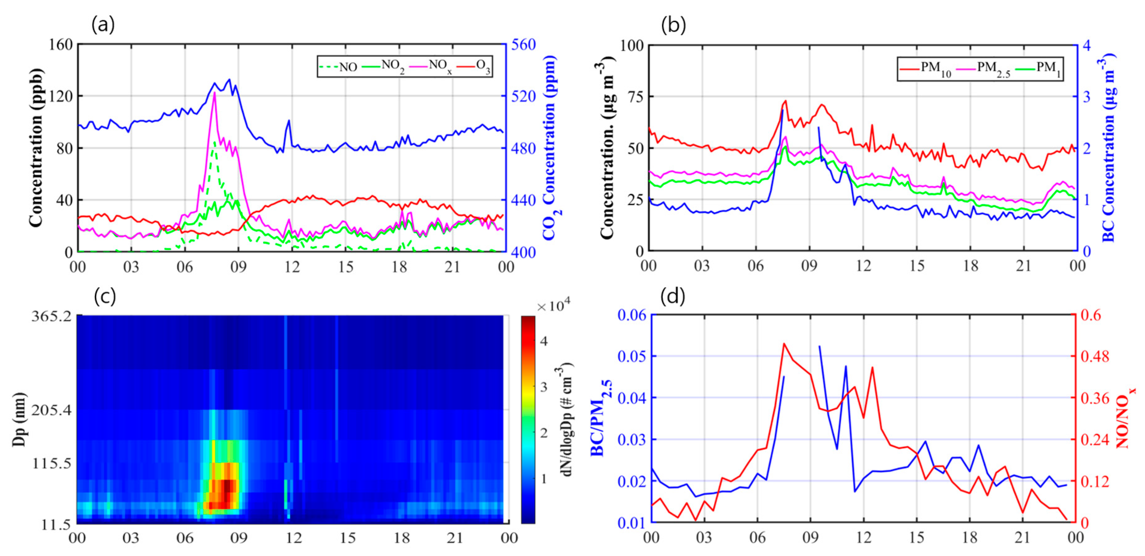
3.1. Diurnal Variations of Near-Road Environments

In the diurnal variations of air temperature and relative humidity observed at the Chuncheon AWS, the lowest average air temperature was –2.9 ℃ (6 a.m.), and the highest average air temperature was 10.0 ℃ (2 p.m.), with a daily temperature difference larger than 10 ℃. The relative humidity exhibited an opposite trend to the air temperature. The diurnal variations of air temperature and relative humidity obviously followed their typical diurnal variation according to the surface heating and cooling. However, the relative humidity temporarily increased in the afternoon on March 12 and 15 because of light precipitation amount of 2–4 mm day−1. The predominant winds for the study periods were northerly and southwesterly winds. Geographically, Chuncheon is located in a basin with a low valley to the southwest and a high ridge to the north. Thus, the mountain-valley wind circulation on clear days in Chuncheon periodically produces a northerly wind at a low wind speed at night and a southwesterly wind at a high wind speed during the day [40,41]. The drone measurements were performed at 8–9 a.m. when the predominant winds were weak southerly-to-southwesterly winds with wind speeds less than 1.3 m s−1, except on March 15 (Table 3). Therefore, the drone and stationary measurement locations were located downwind of the Toegye Intersection, except on March 15. The urban background PM2.5, NO2, and O3 concentrations measured at the AQMS located approximately 1 km away from the intersection showed good or average air quality standard levels except on March 12. In summary, the background meteorological and environmental conditions for the study periods showed typical diurnal variations in spring season, allowing for the identification of near-road air pollution.
The diurnal variations of pollutant concentrations measured on the 11th floor of the apartment building for the P1D and P2D periods are shown in Figure 3. The averaged NOx concentration was the highest at approximately 120 ppb during the morning rush hours (8–9 a.m.), which was 3.5 times higher than the daily-averaged NOx concentration. During the morning rush hours, the concentration of NO primarily emitted from vehicles was over 80 ppb, accounting for most of the NOx. Because the NO emitted from the road reacts with O3 to form NO2, the O3 concentration during the morning rush hours was the lowest during a day [42]. The highest CO2 concentration was also shown during the morning rush hours coinciding with NOx concentration, which is about 40 ppm higher than the lowest one.
The PM10, PM2.5, and PM1 also recorded the highest concentration during the morning rush hours. The highest PM10, PM2.5, and PM1 concentrations exceeded their daily averages by 23%, 35%, and 38%, respectively. Furthermore, the UFP number concentration measured by the SMPS during the morning rush hours was approximately three times higher than its daily average. The emitted particles from a diesel engine are initially UFPs with a diameter less than 100 nm. The emitted particles grow quickly in the atmosphere, and are mostly composed of PM1 within a few minutes [43,44]. The freshly emitted particles from a diesel engine are optically characterized as BC. Therefore, the BC similarly showed an increasing trend during the morning rush hours, and had a 3–6% proportion of PM1, even in the outdoor environment of the apartment building. As a result, the influence of the pollutants emitted on roads directly appeared at the stationary measurement location on 11st floor at 150 m away from the intersection.
In many measurement studies, analyses of concentration ratios between two pollutants have been utilized, both to minimize the effects of other environmental factors such as atmospheric stability and background concentration and to solely examine the effects of vehicle emissions [45,46]. The diurnal variations of NO/NOx and BC/PM2.5 concentration ratios are presented in Figure 3d. The NO/NOx and BC/PM2.5 ratios were 2.7 and at least 2.0 times higher, respectively, during the morning rush hours than their daily averages. Being coincident with the previous results, the effect of pollutants emitted on roads appeared especially large during the morning rush hours, regardless of other environmental factors. By contrast, the diurnal variations of all pollutant concentrations did not show similar increasing phenomena during the evening rush hours. This implies a relatively more effective atmospheric dispersion of emitted pollutants during the evening rush hours than during the morning rush hours, because the wind speeds in the afternoon were mostly higher than 2 m s−1 and the air temperature remained high until the evening hours.

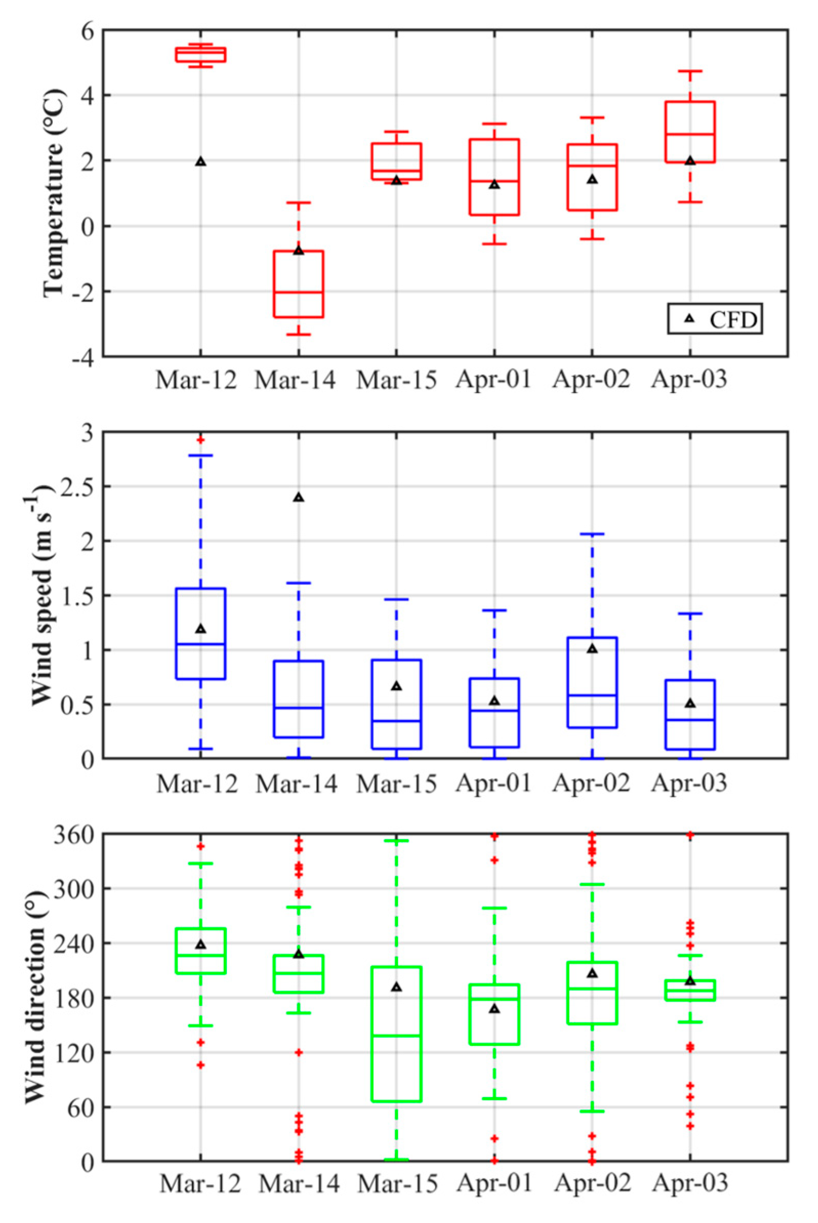
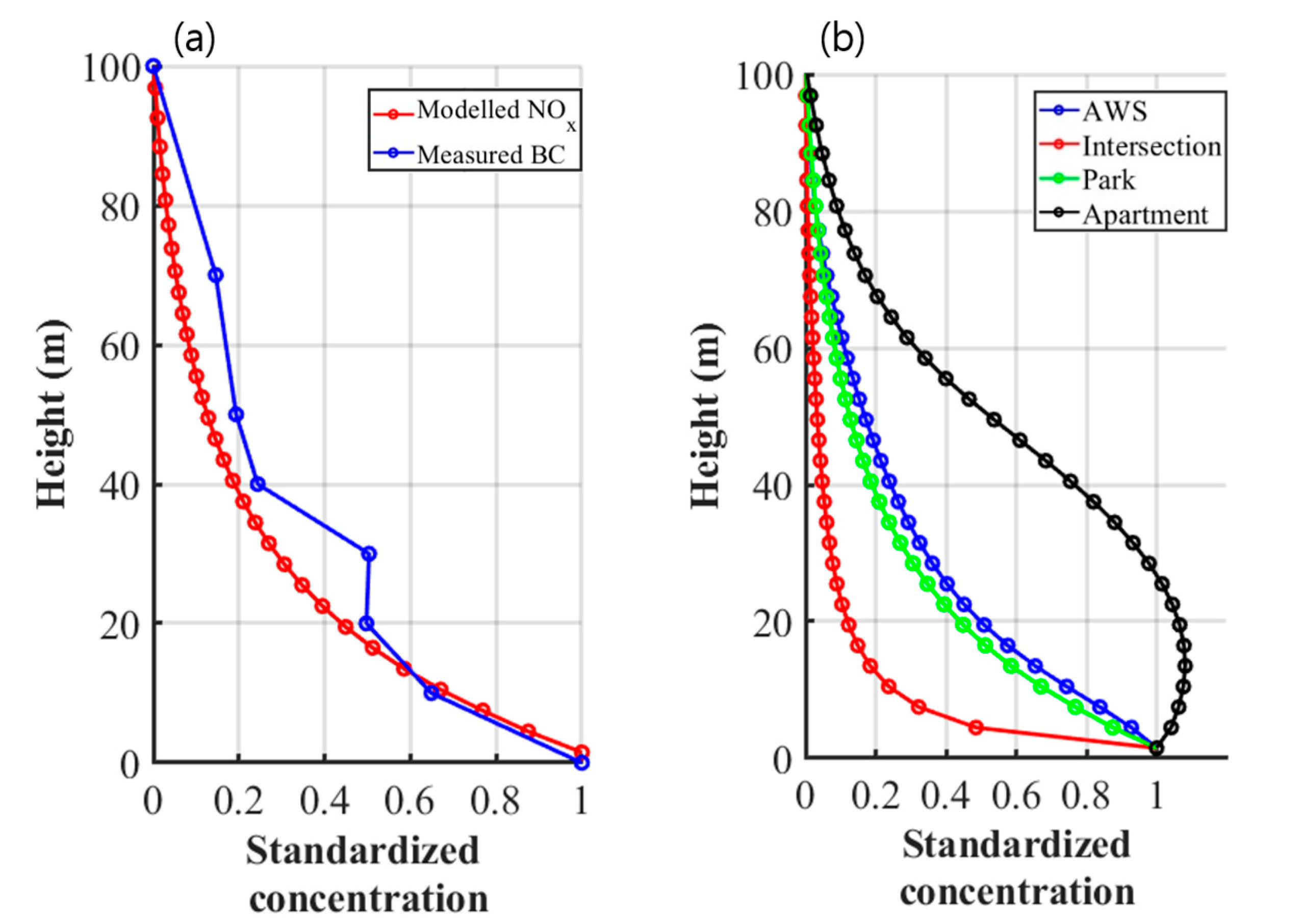
3.2. Verification of WRF-CFD Model

The WRF simulation results were compared with the 1 h interval data observed at the Chuncheon AWS for morning hours (7–10 a.m.). The correlation coefficients between the WRF simulation results and observation data for the P1 period are 0.76 and 0.43 for air temperature and wind speed, respectively, whereas those for the P2 period are relatively higher (0.96 and 0.72 for air temperature and wind speed, respectively). The weather conditions for the P1 period included a couple of precipitation events and cloudy weather. By contrast, the weather conditions for the P2 period showed typically clear weather that continued for a week, which were suitable for an improved simulation performance of the WRF model. In previous studies verifying WRF simulations performed in China, Spain, and India, the correlation coefficients for air temperature and wind speed ranged between 0.78–0.94 and 0.20–0.53, respectively [47,48,49,50]. Their similar values to the results of this study demonstrate that the meteorological inputs provided from the WRF model to the CFD model are appropriate.
The air temperature, wind direction, and wind speed of the CFD simulation results during the morning rush hours were compared with the roadside AWS observation data with a 1-min interval at the Toegye Intersection for the P1D and P2D periods (Figure 4). The air temperature at the roadside location was underestimated in general, with a mean absolute error (MAE) of approximately 1 ℃. The simulated daily lowest air temperature gradually decreased and then increased after March 14, which was in accordance with the AWS observation data. The wind speed at the roadside AWS location was slightly overestimated with an MAE of 0.5 m s−1, showing the simulated wind speed similar to the observed wind speed, except for the strong wind case on March 14. The simulated wind direction at the roadside location was in accordance with the AWS observation data based on the sixteenth classification of wind direction. As a result, the CFD model properly simulated near-road meteorological fields that could reasonably represent air pollution distribution in the CFD model domain.

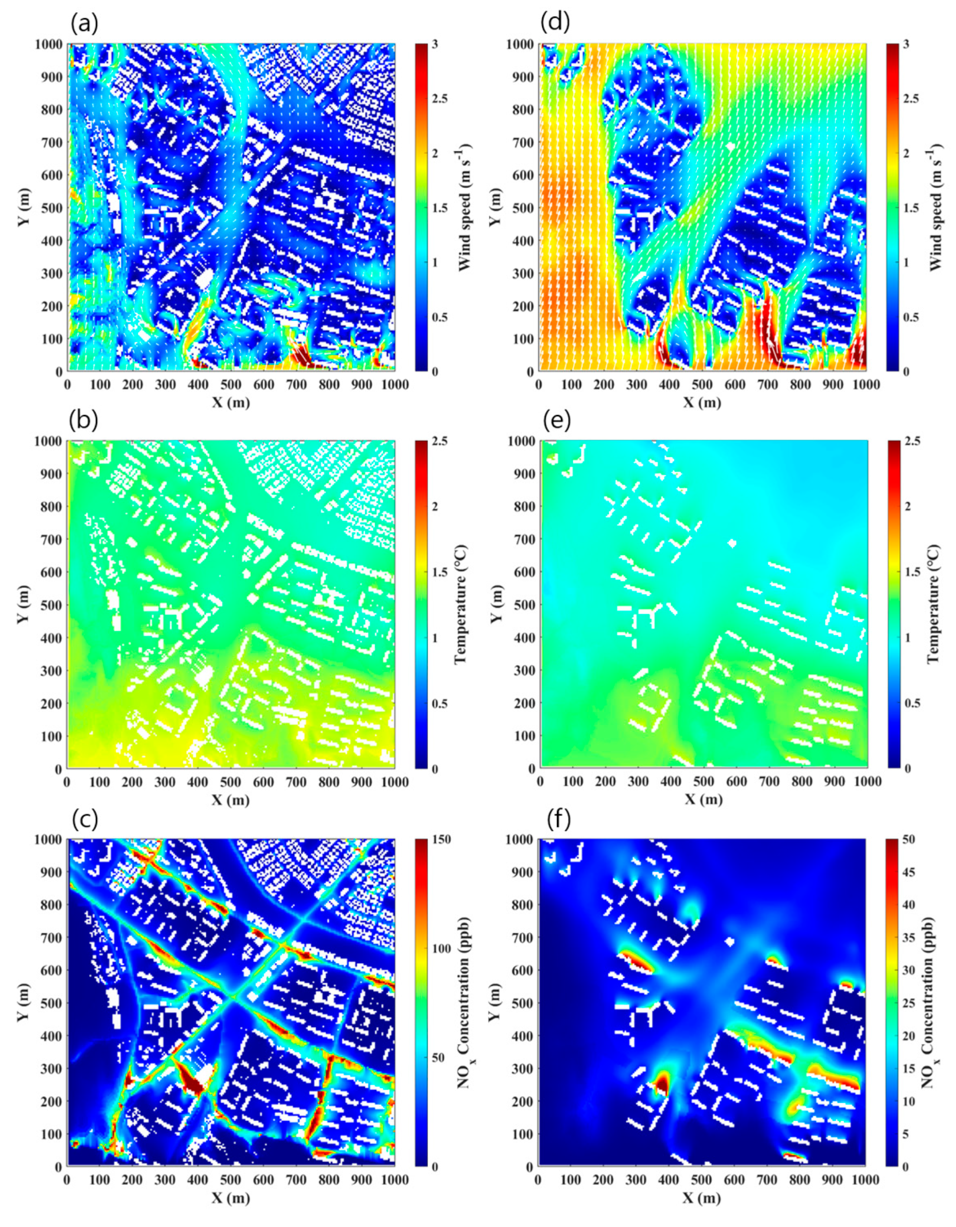
3.3. Spatial Distribution of Near-Road Environments

The simulated horizontal wind, air temperature, and NOx concentration fields at the altitudes of 1.5 and 30 m are compared by averaging their distributions for six days during the P1D and P2D periods in total to identify the typical 3-D extent of traffic-related air pollution around the road intersection (Figure 5). Because of south-to-southwest winds during the study periods, the wind speed at the 1.5 m altitude was relatively high along the stream in the south and the urban park in the north of the intersection. By contrast, the wind speeds in the apartment complexes near the intersection were mostly lower than 1 m s−1 because of the blocking effect produced by the buildings (Figure 5a). The lower wind speeds in the apartment complexes also were shown at the 30 m altitude, which were clearly differentiated from the wind speeds in the rest of domain at the 30 m altitude (Figure 5d). The air temperatures tended to be higher in the apartment complexes compared to those in the rest of domain, while the air temperatures at the 30 m altitude were generally lower than those at the 1.5 m altitude within differences smaller than 0.5 ℃ depending on the location (Figure 5b,e). The NOx concentrations at the 1.5 m altitude near the intersection and road were higher than those in the apartment complexes by 50 ppb or more (Figure 5c). The NOx emitted from the road was more accumulated where the apartment and commercial buildings are elongated perpendicular to the wind direction near the road. The accumulated NOx concentrations behind the buildings for the perpendicular wind direction to the road axis similarly appeared at the 30 m altitude (Figure 5f). The accumulation of NOx emitted on roads is known as the street canyon effect with recirculating flows inside a street canyon especially with a high aspect ratio of building height to street width [51,52]. As a result, the NOx distribution in three dimensions near the road intersection and apartment buildings was greatly influenced by mechanical factors such as geometries and arrangements of road and buildings rather than by thermal factors during the morning rush hours in presence of a weak solar heating on surfaces.
Figure 6 shows y–z vertical cross-sections at x = 207 m and x = 705 m where NOx emitted on roads was apparently accumulated in street canyons. In the presence of the recirculating flows in street canyons as indicated by wind vectors, the emitted NOx from mobile sources on roads is then transported upward to a higher floor along the leeward building walls. Similarly, previous studies [27,53] showed using CFD model simulations that the accumulation of emitted pollutant on roads gradually increases and then maximizes at a 3–10 m altitude from the ground near the roadside building walls because of the upward transport of emitted pollutant. In this study, compared to the previous studies, the maximized concentrations near the roadside building walls frequently appeared at a higher altitude because of taller building heights (i.e., approximately 50 m height). This leads to an increase in personal NOx intake fraction for residents in the apartment buildings [54]. Consequently, high-rise roadside buildings worsen the near-road air quality by accumulating the emitted pollutants on roads not only at a ground level but also at elevated levels because of combination of the accumulation and upward transport along the roadside building walls. This clearly supports the analyzed results of stationary measurements at the 30 m altitude during the morning rush hours.

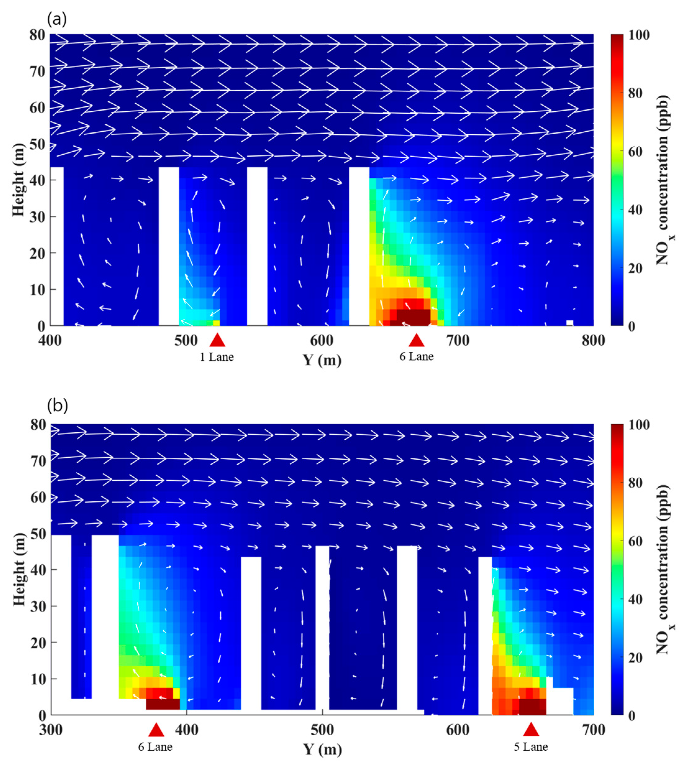
3.4. 3-D Spatial Extent of Near-Road Air Pollution

We measured the vertical distribution of pollutant concentration using a drone and compared the measured result with the simulated one to support the 3-D spatial assessment of near-road air pollution. The measured profiles of air temperature, PM2.5, BC, and O3 concentrations during the morning rush hours for the P1D and P2D periods are shown in Figure 7. The air temperature profile exhibits that the near-surface atmosphere was relatively neutral because surface cooling during the nighttime transits to surface heating after sunrise. The stable-to-neutral atmospheric stability in the early morning is favorable for the accumulation of emitted pollutants near the surface. The PM2.5 concentration profile shows a decreasing trend as the altitude increases with the concentration median of 53 μg m–3 on the ground and 44 μg m–3 at the 100 m altitude. Most vertical variations in PM2.5 concentration appear below the apartment building height, while the PM2.5 concentration is almost uniform above the building height, which is similar to the previous study [55]. The decreasing trend is more apparent in the BC concentration profiles with the concentration median of 3.1 μg m–3 on the ground and 2.2 μg m–3 at the 100 m altitude. The steeper decrease in BC concentration than in PM2.5 concentration is attributed to the large proportion of BC in emitted particles especially in finer particles from vehicles on roads [56,57]. In contrast to PM2.5 and BC concentrations, the O3 concentration profile shows an increasing trend as the altitude increases with the concentration median of 0.027 ppm on the ground and 0.040 ppm at the 100 m altitude. This was a result of atmospheric O3 being actively titrated with NOx emitted on roads. In summary, PM2.5, BC, and O3 all show significant vertical variations in their concentrations below the apartment building height at the downwind location of the road intersection in the urban park. This agrees well with the CFD simulation result showing the worsened air quality in the near-road environment surrounded by high-rise apartment buildings.
BC and NOx are commonly emitted from vehicles and have a strong correlation (R2 ≥ 0.78) in the measurement data during the morning rush hours [58]. Using the drone measurement data, therefore, we verify the accuracy of the CFD simulation results to identify the 3-D spatial extent of near-road air pollution around the intersection. To take the effect of on-road emission into account separately, the standardizing method is adopted for quantitatively comparing the measured BC and simulated NOx concentration profiles to each other by setting them to 1 for the highest concentrations and to 0 for the lowest concentrations [59]. Figure 8a shows the standardized vertical profiles of measured BC and simulated NOx concentrations at the drone measurement location for six days of the P1D and P2D periods. Both the measured BC and simulated NOx concentrations sharply decrease with increasing altitude and are reduced by 50% approximately at the 20 m altitude compared to their highest concentrations on the ground. These similar decreasing trends of the measured BC and simulated NOx concentrations guarantee the reliability of spatial distribution of NOx concentration simulated by the CFD model.
The simulated NOx concentration profiles at selected locations that are the road intersection (Intersection), roadside AWS location (AWS) with a 30 m distance from the intersection, the drone measurement location in the urban park (Park), and the stationary measurement location in the apartment building (Apartment) are shown in Figure 8b. The standardized NOx concentrations at the ‘Park’ and ‘AWS’ locations show similarly decreasing profiles with increasing altitude, while that at the ‘Intersection’ location is almost reduced by 90% approximately at the 20 m altitude compared to the highest concentration on the ground. This is because the emitted NOx at the intersection is mechanically transported horizontally rather than vertically in the presence of no or very weak surface heating on the ground. However, the standardized NOx concentration at the ‘Apartment’ location shows its maximum approximately at the 15 m altitude rather than on the ground because the dispersion effect of plume transported downwind increases the plume height as the horizontal distance from the intersection increases. In addition, the upward transport of emitted NOx along the apartment building wall also contributes to increase the plume height at the ‘Apartment’ location. As a result, the 3-D spatial extent of near-road air pollution is predominantly determined by the wind direction relative to the road axis and layout of roadside buildings.
To estimate the human exposure to traffic-related pollutants not only for pedestrians but also for residents in roadside apartment buildings, a representative 2-D vertical cross-section is composited in terms of the horizontal and vertical distances from the center of intersection using the simulated NOx concentration regardless of direction (Figure 9). The composited NOx concentration in the 2-D vertical cross-section is the highest at 76 ppb at the center of intersection, and then gradually decreases by 50% at a 50 m horizontal distance on the ground corresponding to the drone measurement location and by almost 90% at a 150 m horizontal and a 30 m vertical distance corresponding to the stationary measurement location of apartment building. The composited NOx concentration at a certain altitude decreases, as the horizontal distance from the center of intersection increases up to a 120 m. Meanwhile, the composited NOx concentration shows secondary peaks at the horizontal distances of approximately 200 m and 270 m from the center of intersection which is sufficiently far from the intersection because of NOx emission on nearby roads. In conclusion, the horizontal extent of near-road air pollution around the intersection is at least 120 m or, to some directions, 200 m from the center of intersection. The vertical extent of near-road air pollution around the intersection is at least a half of roadside building height or possibly higher up to the roadside building height in the downwind direction.

4. Conclusions

The 3-D spatial extent of the near-road air pollution around the intersection in an urban residential area was investigated using two complementary methods that are drone monitoring and WRF-CFD modeling. Based on the stationary measurement data collected on 11th floor of the roadside apartment building (i.e., 30 m height), we focused on the morning rush hours when the measured concentrations of traffic-related air pollutants such as NOx, BC, and UFP were maximized during a day. The WRF-CFD model simulated the NOx concentration fields around the intersection during the morning rush hours. The simulated highest concentration appeared on roads between roadside apartment buildings, which was attributed to the accumulation of emitted NOx following recirculating flows inside street canyons when the prevailing wind direction was almost perpendicular to the street canyon. The drone measurement conducted close to the road intersection showed decreasing trends in the measured BC and PM2.5 concentrations with increasing altitude. The vertical gradient of measured BC concentration was steeper than that of measured PM2.5 concentration because BC has a large portion in emitted particles from vehicles. The vertical concentration gradients of all measured pollutants including BC, PM2.5, and O3 became insignificant at altitudes higher than the apartment building height (i.e., 50 m height), implying the weakened pollutant dispersion and worsened air quality in building canopies. The standardized BC concentration measured using the drone and NOx concentration simulated using the WRF-CFD model were inter-compared and matched closely with each other especially near ground levels. Consequently, the spatial extents of near-road air pollution adversely affecting the health of pedestrians and residents covered at least 120 m distance from the center of intersection horizontally and at least a half of building height vertically, but in some cases, up to the nearby road network and to the top floor of building. More importantly, the 3-D spatial extent of near-road air pollution was determined by the atmospheric transport governed by the building arrangement and prevailing winds in the urban residential area.
The estimated spatial extent of air pollution using drone monitoring and WRF-CFD modeling is a site-specific result that can be further extended in other urban residential areas with larger traffic emissions and more complicated building geometries. In this study, it is assumed that there is no pollutant emission in the CFD model domain other than road traffic, which is idealistic condition. In a complicated atmospheric environment, various pollutant sources, such as residential heating, industrial complexes, and biomass burning, need to be incorporated for assessing the realistic spatial distribution of air pollutants. The main achievement of this study is, first, the comparability of two complementary methods for examining the spatiotemporal variabilities of local-scale air quality. In addition, the standardized measured and simulated concentrations can be further interpreted as representative local air quality profiles near air pollution hotspots, such as main roads and intersections, for planning and assessing environmental policy on urban air quality.

Author Contributions

Methodology, validation, formal analysis, investigation, data curation, writing—original draft preparation, and visualization: S.-H.L.; Conceptualization, writing—review and editing, supervision, project administration, and funding acquisition: K.-H.K. All authors have read and agreed to the published version of the manuscript.

Funding

This research was funded by Basic Science Research Program through the National Research Foundation of Korea (NRF) funded by the Ministry of Science and ICT (NRF-2017R1C1B2010509 and NRF-2020R1C1C1012354).

Conflicts of Interest

The authors declare no conflict of interest.

References

  1. United Nations, Department of Economic and Social Affairs, Population Division. World Urbanization Prospects: The 2018 Revision (ST/ESA/SER.A/420); United Nations: New York, NY, USA, 2019; p. 103. [Google Scholar]
  2. Patel, M.M.; Chillrud, S.N.; Correa, J.C.; Feinberg, M.; Hazi, Y.; Deepti, K.C.; Prakash, S.; Ross, J.M.; Levy, D.; Kinney, P.L. Spatial and temporal variations in traffic-related particulate matter at New York City high schools. Atmos. Environ. 2009, 43, 4975–4981. [Google Scholar] [CrossRef] [PubMed] [Green Version]
  3. Xing, Y.; Brimblecombe, P. Urban park layout and exposure to traffic-derived air pollutants. Land. Urban Plan. 2020, 194, 103682. [Google Scholar] [CrossRef]
  4. Schikowski, T.; Sugiri, D.; Ranft, U.; Gehring, U.; Heinrich, J.; Wichmann, H.-E.; Krämer, U. Long-term air pollution exposure and living close to busy roads are associated with COPD in women. Respir. Res. 2005, 6, 152. [Google Scholar] [CrossRef] [Green Version]
  5. Amram, O.; Abernethy, R.; Brauer, M.; Davies, H.; Allen, R.W. Proximity of public elementary schools to major roads in Canadian urban areas. Int. J. Health Geo. 2011, 10, 68. [Google Scholar] [CrossRef] [Green Version]
  6. Zhu, X.; Fan, Z.; Wu, X.; Meng, Q.; Wang, S.; Tang, X.; Ohman-Strickland, P.; Georgopoulos, P.; Zhang, J.; Bonanno, L.; et al. Spatial variation of volatile organic compounds in a “Hot Spot” for air pollution. Atmos. Environ. 2008, 42, 7329–7338. [Google Scholar] [CrossRef] [PubMed] [Green Version]
  7. Goel, A.; Kumar, P. A review of fundamental drivers governing the emissions, dispersion and exposure to vehicle-emitted nanoparticles at signalised traffic intersections. Atmos. Environ. 2014, 97, 316–331. [Google Scholar] [CrossRef] [Green Version]
  8. Várhelyi, A. The effects of small roundabouts on emissions and fuel consumption: A case study. Transport. Res. Part D 2002, 7, 65–71. [Google Scholar] [CrossRef]
  9. Coelho, M.C.; Farias, T.L.; Rouphail, N.M. Impact of speed control traffic signals on pollutant emissions. Transport. Res. Part D 2005, 10, 323–340. [Google Scholar] [CrossRef]
  10. Pandian, S.; Gokhale, S.; Ghoshal, A.K. Evaluating effects of traffic and vehicle characteristics on vehicular emissions near traffic intersections. Transport. Res. Part D 2009, 14, 180–196. [Google Scholar] [CrossRef]
  11. Britter, R.E.; Hanna, S.R. Flow and dispersion in urban areas. Ann. Rev. Fluid Mech. 2003, 35, 469–496. [Google Scholar] [CrossRef]
  12. Kwak, K.-H.; Woo, S.H.; Kim, K.H.; Lee, S.-B.; Bae, G.-N.; Ma, Y.-I.; Sunwoo, Y.; Baik, J.-J. On-road air quality associated with traffic composition and street-canyon ventilation: Mobile monitoring and CFD modeling. Atmosphere 2018, 9, 92. [Google Scholar] [CrossRef] [Green Version]
  13. Faus-Kessler, T.; Kirchner, M.; Jakobi, G. Modelling the decay of concentrations of nitrogenous compounds with distance from roads. Atmos. Environ. 2008, 42, 4589–4600. [Google Scholar] [CrossRef]
  14. Naser, T.M.; Kanda, I.; Ohara, T.; Sakamoto, K.; Kobayashi, S.; Nitta, H.; Nataami, T. Analysis of traffic-related NOx and EC concentrations at various distances from major roads in Japan. Atmos. Environ. 2009, 43, 2379–2390. [Google Scholar] [CrossRef]
  15. Choi, W.; Winer, A.M.; Paulson, S.E. Factors controlling pollutant plume length downwind of major roadways in nocturnal surface inversions. Atmos. Chem. Phys. 2014, 14, 6925–6940. [Google Scholar] [CrossRef] [Green Version]
  16. Xing, Y.; Brimblecombe, P. Dispersion of traffic derived air pollutants into urban parks. Sci. Tot. Environ. 2018, 622–623, 576–583. [Google Scholar] [CrossRef]
  17. Goel, A.; Kumar, P. Vertical and horizontal variability in airborne nanoparticles and their exposure around signalised traffic intersections. Environ. Pollut. 2016, 214, 54–69. [Google Scholar] [CrossRef]
  18. Sajani, S.Z.; Marchesi, S.; Trentini, A.; Bacco, D.; Zigola, C.; Rovelli, S.; Ricciardelli, I.; Maccone, C.; Lauriola, P.; Cavallo, D.M.; et al. Vertical variation of PM2.5 mass and chemical composition, particle size distribution, NO2, and BTEX at a high rise building. Environ. Pollut. 2018, 235, 339–349. [Google Scholar] [CrossRef]
  19. Azimi, P.; Zhao, H.; Fazli, T.; Zhao, D.; Faramarzi, A.; Leung, L.; Stephens, B. Pilot study of the vertical variations in outdoor pollutant concentrations and environmental conditions along the height of a tall building. Build. Environ. 2018, 138, 124–134. [Google Scholar] [CrossRef]
  20. Villa, T.F.; Jayaratne, E.R.; Gonzalez, L.F.; Morawska, L. Determination of the vertical profile of particle number concentration adjacent to a motorway using an unmanned aerial vehicle. Environ. Pollut. 2017, 230, 134–142. [Google Scholar] [CrossRef] [Green Version]
  21. Liu, F.; Zheng, X.; Qian, H. Comparison of particle concentration vertical profiles between downtown and urban forest park in Nanjing (China). Atmos. Pollut. Res. 2018, 9, 829–839. [Google Scholar] [CrossRef]
  22. Solazzo, E.; Vardoulakis, S.; Cai, X. A novel methodology for interpreting air quality measurements from urban streets using CFD modelling. Atmos. Environ. 2011, 45, 5230–5239. [Google Scholar] [CrossRef]
  23. Lateb, M.; Meroney, R.N.; Yataghene, M.; Fellouah, H.; Saleh, F.; Boufadel, M.C. On the use of numerical modelling for near-field pollutant dispersion in urban environments—A review. Environ. Pollut. 2016, 208, 271–283. [Google Scholar] [CrossRef] [PubMed] [Green Version]
  24. Li, B.; Li, X.-B.; Li, C.; Zhu, Y.; Peng, Z.-R.; Wang, Z.; Lu, S.-J. Impacts of wind fields on the distribution patterns of traffic emitted particles in urban residential areas. Transport. Res. Part D 2019, 68, 122–136. [Google Scholar] [CrossRef]
  25. Aristodemou, E.; Boganegra, L.M.; Mottet, L.; Pavlidis, D.; Constantinou, A.; Pain, C.; Robins, A.; ApSimon, H. How tall buildings affect turbulent air flows and dispersion of pollution within a neighbourhood. Environ. Pollut. 2018, 233, 782–796. [Google Scholar] [CrossRef]
  26. Yang, B.; Gu, J.; Zhang, T.; Zhang, K. M Near-source air quality impact of a distributed natural gas combined heat and power facility. Environ. Pollut. 2019, 246, 650–657. [Google Scholar] [CrossRef]
  27. Karkoulias, V.A.; Marazioti, P.E.; Georgiou, D.P.; Maraziotis, E.A. Computational fluid dynamics modeling of the trace elements dispersion and comparison with measurements in a street canyon with balconies in the city of Patras, Greece. Atmos. Environ. 2020, 223, 117210. [Google Scholar] [CrossRef]
  28. Efthimiou, G.C.; Berbekar, E.; Harms, F.; Bartzis, J.G.; Leitl, B. Prediction of high concentrations and concentration distribution of a continuous point source release in a semi-idealized urban canopy using CFD-RANS modeling. Atmos. Environ. 2015, 100, 48–56. [Google Scholar] [CrossRef]
  29. Baik, J.-J.; Park, S.-B.; Kim, J.-J. Urban flow and dispersion simulation using a CFD model coupled to a mesoscale model. J. Appl. Meteor. Clim. 2009, 48, 1667–1681. [Google Scholar] [CrossRef]
  30. Tewari, M.; Kusaka, H.; Chen, F.; Coirier, W.J.; Kim, S.; Wyszogrodzki, A.A.; Warner, T.T. Impact of coupling a microscale computational fluid dynamics model with a mesoscale model on urban scale contaminant transport and dispersion. Atmos. Res. 2010, 96, 656–664. [Google Scholar] [CrossRef]
  31. Kwak, K.-H.; Baik, J.-J.; Ryu, Y.-H.; Lee, S.-H. Urban air quality simulation in a high-rise building area using a CFD model coupled with mesoscale meteorological and chemistry-transport models. Atmos. Environ. 2015, 100, 167–177. [Google Scholar] [CrossRef]
  32. Kadaverugu, R.; Sharma, A.; Matli, C.; Biniwale, R. High resolution urban air quality modeling by coupling CFD and mesoscale models: A review. Asia Pac. J. Atmos. Sci. 2019, 55, 539–556. [Google Scholar] [CrossRef]
  33. Oh, H.-S.; Lee, S.-H.; Choi, D.-W.; Kwak, K.-H. Comparison of the vertical PM2.5 distributions according to atmospheric stability using a drone during open burning events. J. Korean Soc. Atmos. Environ. 2020, 36, 108–118. [Google Scholar] [CrossRef]
  34. Brady, J.M.; Stokes, M.D.; Bonnardel, J.; Bertram, T.H. Characterization of a quadrotor unmanned aircraft system for aerosol-particle-concentration measurements. Environ. Sci. Tech. 2016, 50, 1376–1383. [Google Scholar] [CrossRef] [PubMed]
  35. Hong, S.-Y.; Noh, Y.; Dudhia, J. A new vertical diffusion package with an explicit treatment of entrainment processes. Mon. Weath. Rev. 2006, 134, 2318–2341. [Google Scholar] [CrossRef] [Green Version]
  36. Janjic, Z.A. The step-mountain coordinate: Physics package. Mon. Weath. Rev. 1990, 118, 1429–1443. [Google Scholar] [CrossRef]
  37. Baik, J.-J.; Kim, J.-J.; Fernando, H.J.S. A CFD model for simulating urban flow and dispersion. J. Appl. Meteorol. 2003, 42, 1636–1648. [Google Scholar] [CrossRef]
  38. Rivas, E.; Santiago, J.L.; Lechón, Y.; Martín, F.; Ariño, A.; Pons, J.J.; Santamaría, J.M. CFD modelling of air quality in Pamplona City (Spain): Assessment, stations spatial representativeness and health impacts valuation. Sci. Tot. Environ. 2019, 649, 1362–1380. [Google Scholar] [CrossRef]
  39. Fu, X.; Xiang, S.; Liu, Y.; Liu, J.; Yu, J.; Mauzerall, D.L.; Tao, S. High-resolution simulation of local traffic-related NOx dispersion and distribution in a complex urban terrain. Environ. Pollut. 2020, 263, 114390. [Google Scholar] [CrossRef]
  40. Lee, H.W.; Lee, K.O.; Baek, S.-J.; Kim, D.H. Analysis of meteorological features and prediction probability associated with the fog occurrence at Chuncheon. J. Korean Soc. Atmos. Environ. 2005, 21, 303–313. [Google Scholar]
  41. Shim, H.-N.; Lee, Y.-H. Influence of local wind on occurrence of fog at inland areas. Atmosphere 2017, 27, 213–224. [Google Scholar]
  42. Kwak, K.-H.; Lee, S.-H.; Seo, J.M.; Park, S.-B.; Baik, J.-J. Relationship between rooftop and on-road concentrations of traffic-related pollutants in a busy street canyon: Ambient wind effects. Environ. Pollut. 2016, 208, 185–197. [Google Scholar] [CrossRef] [PubMed]
  43. Kittelson, D.B. Engines and nanoparticles: A review. J. Aeros. Sci. 1998, 29, 575–588. [Google Scholar] [CrossRef]
  44. Kumar, P.; Morawska, L.; Birmili, W.; Paasonen, P.; Hu, M.; Kulmala, M.; Harrison, R.M.; Norford, L.; Britter, R. Ultrafine particles in cities. Environ. Int. 2014, 66, 1–10. [Google Scholar] [CrossRef] [PubMed] [Green Version]
  45. Kimbrough, S.; Owen, R.C.; Snyder, M.; Richmond-Bryant, J. NO to NO2 conversion rate analysis and implications for dispersion model chemistry methods using Las Vegas, Nevada near-road field measurements. Atmos. Environ. 2017, 165, 23–34. [Google Scholar] [CrossRef] [PubMed]
  46. Liu, Y.; Yan, C.; Zheng, M. Source apportionment of black carbon during winter in Beijing. Sci. Tot. Environ. 2018, 618, 531–541. [Google Scholar] [CrossRef] [PubMed]
  47. Pan, X.; Li, X.; Shi, X.; Han, X.; Luo, L.; Wang, L. Dynamic downscaling of near-surface air temperature at the basin scale using WRF-a case study in the Heihe river basin, China. Front. Earth Sci. 2012, 6, 314–323. [Google Scholar] [CrossRef]
  48. Banks, R.F.; Baldasano, J.M. Impact of WRF model PBL schemes on air quality simulations over Catalonia, Spain. Sci. Tot. Environ. 2016, 572, 98–113. [Google Scholar] [CrossRef] [Green Version]
  49. Boadh, R.; Satyanarayana, A.N.V.; Krishna, T.V.B.P.S.R.; Madala, S. Sensitivity of PBL schemes of the WRF-ARW model in simulating the boundary layer flow parameters for their application to air pollution dispersion modeling over a tropical station. Atmosphere 2016, 29, 61–81. [Google Scholar] [CrossRef] [Green Version]
  50. Avolio, E.; Federico, S.; Miglietta, M.M.; Feudo, T.L.; Calidonna, C.R.; Sempreviva, A.M. Sensitivity analysis of WRF model PBL schemes in simulating boundary-layer variables in southern Italy: An experimental campaign. Atmos. Res. 2017, 192, 58–71. [Google Scholar] [CrossRef]
  51. He, L.; Hang, J.; Wang, X.; Lin, B.; Li, X.; Lan, G. Numerical investigations of flow and passive pollutant exposure in high-rise deep street canyons with various street aspect ratios and viaduct settings. Sci. Tot. Environ. 2017, 584, 189–206. [Google Scholar] [CrossRef]
  52. Zhang, K.; Chen, G.; Wang, X.; Liu, S.; Mak, C.M.; Fan, Y.; Hang, J. Numerical evaluations of urban design technique to reduce vehicular personal intake fraction in deep street canyons. Sci. Tot. Environ. 2019, 653, 968–994. [Google Scholar] [CrossRef] [PubMed]
  53. Thaker, P.; Gokhale, S. The impact of traffic-flow patterns on air quality in urban street canyons. Environ. Pollut. 2016, 208, 161–169. [Google Scholar] [CrossRef] [PubMed]
  54. Hang, J.; Luo, Z.; Wang, X.; He, L.; Wang, B.; Zhu, W. The influence of street layouts and viaduct settings on daily carbon monoxide exposure and intake fraction in idealized urban canyons. Environ. Pollut. 2017, 220, 72–86. [Google Scholar] [CrossRef] [PubMed]
  55. Kuuluvainen, H.; Poikkimäki, M.; Järvinen, A.; Kuula, J.; Irjala, M.; Maso, M.D.; Keskinen, J.; Timonen, H.; Niemi, J.V.; Rönkkö, T. Vertical profiles of lung deposited surface area concentration of particulate matter measured with a drone in a street canyon. Environ. Pollut. 2018, 241, 96–105. [Google Scholar] [CrossRef]
  56. Taheri, A.; Aliasghari, P.; Hosseini, V. Black carbon and PM2.5 monitoring campaign on the roadside and residential urban background sites in the city of Tehran. Atmos. Environ. 2019, 218, 116928. [Google Scholar] [CrossRef]
  57. Liu, X.; Schnelle-Kreis, J.; Zhang, X.; Bendl, J.; Khedr, M.; Jakobi, G.; Schloter-Hai, B.; Hovorka, J.; Zimmermann, R. Integration of air pollution data collected by mobile measurement to derive a preliminary spatiotemporal air pollution profile from two neighboring German-Czech border villages. Sci. Tot. Environ. 2020, 722, 137632. [Google Scholar] [CrossRef] [PubMed]
  58. Petetin, H.; Beekmann, M.; Colomb, A.; Denier van der Gon, H.A.C.; Dupont, J.-C.; Honoré, C.; Michoud, V.; Morille, Y.; Perrussel, O.; Schwarzenboeck, A.; et al. Evaluating BC and NOx emission inventories for the Paris region from MEGAPOLI aircraft measurements. Atmos. Chem. Phys. 2015, 15, 9799–9818. [Google Scholar] [CrossRef] [Green Version]
  59. Yuan, C.; Shan, R.; Zhang, Y.; Li, X.-X.; Yin, T.; Hang, J.; Norford, L. Multilayer urban canopy modelling and mapping for traffic pollutant dispersion at high density urban areas. Sci. Tot. Environ. 2019, 647, 255–267. [Google Scholar] [CrossRef]
Figure 1. Measurement locations near the Toegye Intersection in Chuncheon, Gangwon Province, Republic of Korea. The map at the left bottom corner shows the entire Chuncheon basin. The Chuncheon AWS (automatic weather station) and the AQMS (air quality monitoring station) are located at approximately 5 km north and 1 km northeast of the intersection, respectively.
Ijerph 17 06915 g001
Figure 2. (a) Four nested domains in the WRF model and (b) a CFD model domain including the Toegye Intersection and the surrounding apartment and commercial buildings.
Ijerph 17 06915 g002
Figure 3. Time series of (a) gaseous pollutant (NOx, NO, NO2, O3, and CO2) concentrations, (b) particulate pollutant (PM10, PM2.5, PM1, and BC) concentrations, (c) size distributions of UFPs, and (d) concentration ratios (BC/PM2.5 and NO/NOx) measured at the stationary measurement location averaged over the P1D and P2D periods. The average time interval is 10 min except for the concentration ratios (30 min).
Ijerph 17 06915 g003
Figure 4. Boxplots of air temperature, wind speed, and wind direction of AWS observation data compared with CFD simulation results at the roadside location of Toegye Intersection. The number of data point is 60 min × 6 days (n = 360).
Ijerph 17 06915 g004
Figure 5. Simulated six-day averaged horizontal (a) wind speed, (b) air temperature, and (c) NOx concentration fields at a 1.5 m altitude and horizontal (d) wind speed, (e) air temperature, and (f) NOx concentration fields at a 30 m altitude during the P1D and P2D periods.
Ijerph 17 06915 g005
Figure 6. The y-z vertical cross-sections of simulated NOx concentration fields at (a) x = 207 m and (b) x = 705 m. The arrows indicate the wind vectors of v and w components.
Ijerph 17 06915 g006
Figure 7. Vertical profiles of (a) air temperature, (b) PM2.5, (c) BC, and (d) O3 concentration boxplots for six days of P1D and P2D periods. A number of measurement data is 18 per each altitude.
Ijerph 17 06915 g007
Figure 8. Standardized vertical profiles of (a) simulated NOx and measured BC concentrations at the drone measurement location and (b) simulated NOx concentrations at selected locations (i.e., AWS, Intersection, Park, and Apartment) around the road intersection.
Ijerph 17 06915 g008
Figure 9. Composited cross-section of simulated NOx concentration in terms of distances from the intersection at a model grid interval regardless of direction. Green and red markers denote the drone and stationary measurement locations, respectively.
Ijerph 17 06915 g009
Table 1. Specifications of instruments used for drone and stationary measurements.
VariableModel and ManufacturerMeasurement ResolutionAccuracyTime Interval
DronePM2.5Sidepak AM520, TSI (MN, USA)1 μg m−3-1 s
Black carbon (BC)MA200, Aethlab (CA, USA)0.001 μg m−3-5 s
O3Aeroqual 500, Aeroqual (Auckland, NZ)0.001 ppm±0.008 ppm1 min
Air temperature
Relative humidity (RH)
Imet-XQ2, InterMet (MI, USA)0.01 ℃, 0.1%±0.3 ℃, ±5%1 s
StationaryPM10, PM2.5, PM1Model 1.109A, Grimm (NC, USA)0.1 μg m−3±5%6 s
Particle numberNanoscan SMPS3910, TSI (MN, USA)100 particles cm−3-1 min
BCMA200, Aethlab0.001 μg m−3-1 min
NOx, NO2, NOnCLD AL, Eco Physics
(Duernten, Switzerland)
0.001 ppm-1 s
CO2CO2 analyzer, KINSCO technology
(Seoul, ROK)
1 ppm-1 min
O3O3 analyzer, KINSCO technology
(Seoul, ROK)
0.001 ppm-1 min
Table 2. NOx emission factors classified by vehicle type in CAPSS (v = driving speed).
Vehicle TypeFuelEmission Factor (g km−1)
Regular carGasoline ( 3.5 × 10 6 ) v 2 + 0.00033 v + 0.0112
SUV, Light truckDiesel 14.2 × v 0.7747
TaxiLPG 0.000004 v 2 + 0.0006 v + 0.0055
City busCNG 8.6972 × e 0.0130 v
Express busDiesel 40.9398 × v 0.5611
Heavy duty vehicleDiesel 107.5 × v 0.5679
Table 3. Daily meteorological and urban air quality data during the morning rush hours (8–9 a.m.) for the P1D and P2D periods. The wind direction increases clockwise from 0° (i.e., due north). The daily precipitation amounts are indicated together with the precipitation time.
Temp.
(℃)
Wind Speed
(m s−1)
Wind Direction
(°)
Daily
Precipitation
(mm)
Cloud Cover
(1/10)
PM2.5
(μg m−3)
NO2
(ppb)
O3
(ppb)
P1DMar-125.31.32282.4 (10 a.m.–4 p.m.)9452137
Mar-14−1.70.6217-023327
Mar-151.90.5974.0 (3–11 p.m.)10301422
P2DApr-011.50.5164-0233010
Apr-021.60.7207-022828
Apr-032.80.4189-0231228

