Estimating Mangrove Above-Ground Biomass Loss Due to Deforestation in Malaysian Northern Borneo between 2000 and 2015 Using SRTM and Landsat Images


 , , ,
, , ,
Abstract
:1. Introduction
2. Materials and Methods
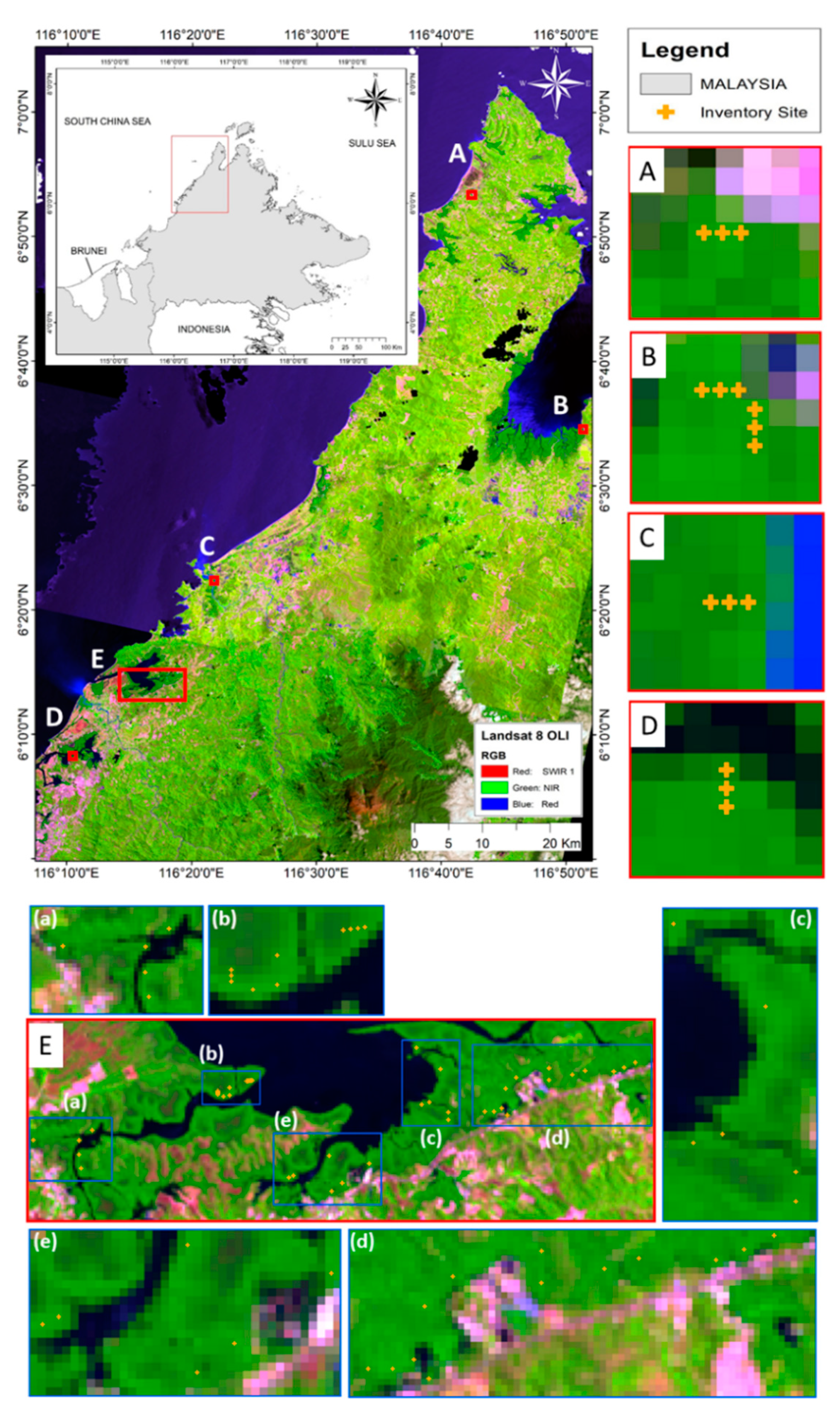
2.1. Study Area
2.2. Field Inventory and AGB Data
2.3. Land Cover Classification of Multi-Temporal Landsat Images
2.4. Canopy Height Models from the SRTM Data
2.5. AGB Prediction Models
3. Results
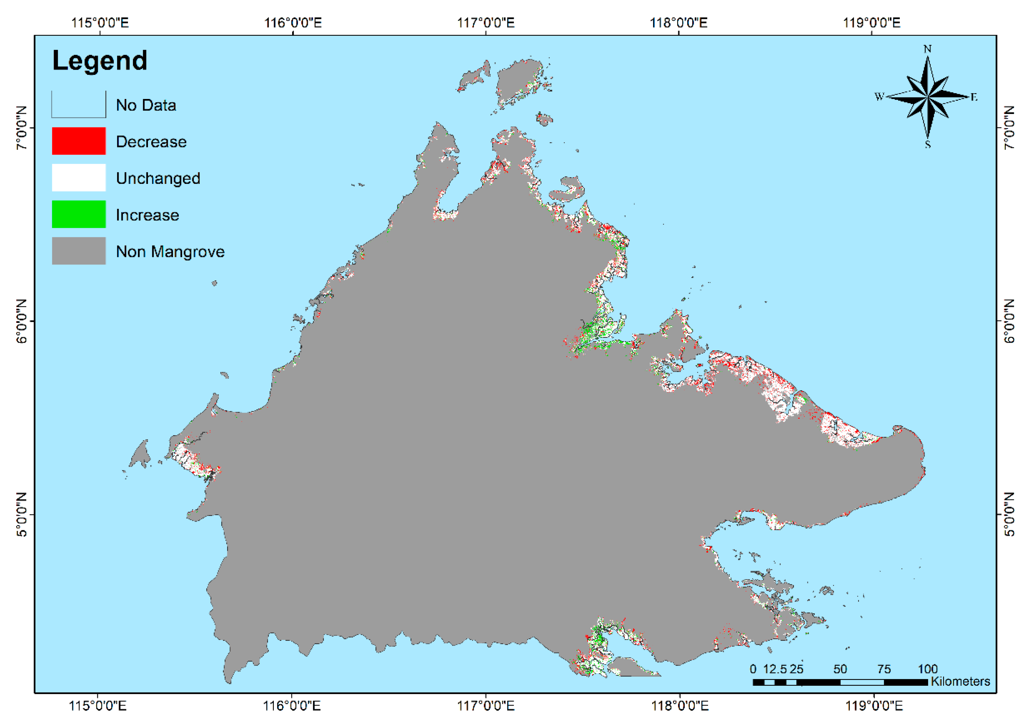
3.1. Mangrove Forest Distribution
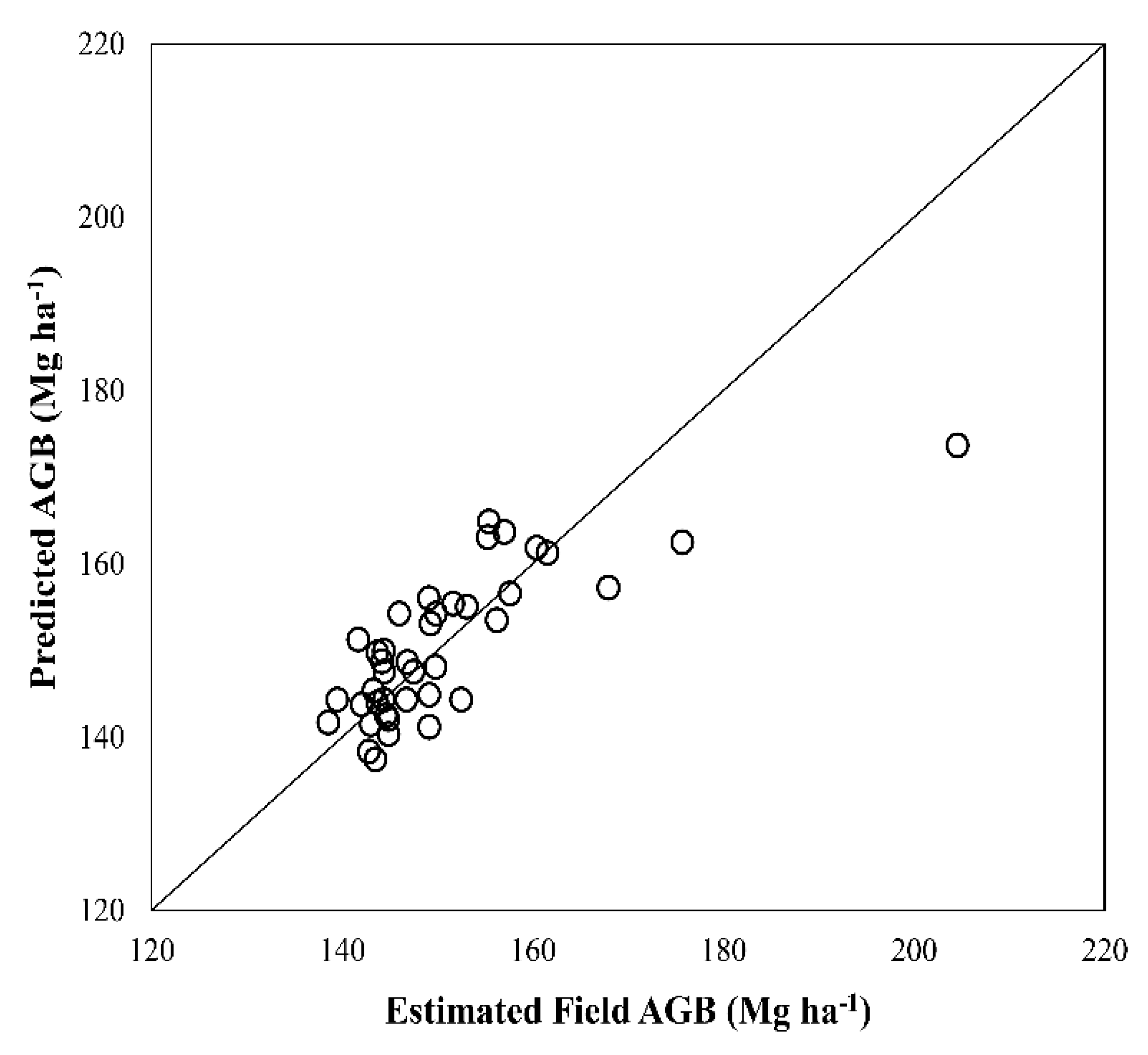
3.2. AGB Estimation
4. Discussion
4.1. Mangrove AGB Estimation Using Remotely Sensed Data
4.2. Mangrove AGB Loss and Its Implications for REDD+ in Sabah, Malaysia
5. Conclusions
Author Contributions
Funding
Acknowledgments
Conflicts of Interest
References
- Baccini, A.; Goetz, S.J.; Walker, W.S.; Laporte, N.T.; Sun, M.; Sulla-Menashe, D.; Hackler, J.; Beck, P.S.A.; Dubayah, R.; Friedl, M.A.; et al. Estimated carbon dioxide emissions from tropical deforestation improved by carbon-density maps. Nat. Clim. Chang. 2012, 2, 182–185. [Google Scholar] [CrossRef]
- UN-REDD. The UN-REDD Programme Strategy 2011–2015; UN-REDD: Geneva, Switzerland, 2011. [Google Scholar]
- Gibbs, H.K.; Brown, S.; Niles, J.O.; Foley, J.A. Monitoring and estimating tropical forest carbon stocks: Making REDD a reality. Environ. Res. Lett. 2007, 2, 1–3. [Google Scholar] [CrossRef]
- UNFCCC. Executive Board Annual Report 2014: Clean Development Mechanism; United Nations Framework Convention on Climate Change: Luxembourg, 2014. [Google Scholar]
- Dahdouh-Guebas, F. World Atlas of Mangroves: Mark Spalding, Mami Kainuma and Lorna Collins (eds). Hum. Ecol. 2011, 39, 107–109. [Google Scholar] [CrossRef]
- Castillo, J.A.A.; Apan, A.A.; Maraseni, T.N.; Salmo, S.G. Soil C quantities of mangrove forests, their competing land uses, and their spatial distribution in the coast of Honda Bay, Philippines. Geoderma 2017, 293, 82–90. [Google Scholar] [CrossRef]
- Donato, D.C.; Kauffman, J.B.; Murdiyarso, D.; Kurnianto, S.; Stidham, M.; Kanninen, M. Mangroves among the most carbon-rich forests in the tropics. Nat. Geosci. 2011, 4, 293–297. [Google Scholar] [CrossRef]
- Pham, L.T.H.; Brabyn, L. Monitoring mangrove biomass change in Vietnam using SPOT images and an object-based approach combined with machine learning algorithms. ISPRS J. Photogramm. Remote Sens. 2017, 128, 86–97. [Google Scholar] [CrossRef]
- Kauffman, J.B.; Heider, C.; Cole, T.G.; Dwire, K.A.; Donato, D.C. Ecosystem carbon stocks of Micronesian mangrove forests. Wetlands 2011, 31, 343–352. [Google Scholar] [CrossRef]
- Stringer, C.E.; Trettin, C.C.; Zarnoch, S.J.; Tang, W. Carbon stocks of mangroves within the Zambezi River Delta, Mozambique. For. Ecol. Manag. 2015, 354, 139–148. [Google Scholar] [CrossRef]
- Kanniah, K.D.; Sheikhi, A.; Cracknell, A.P.; Goh, H.C.; Tan, K.P.; Ho, C.S.; Rasli, F.N. Satellite images for monitoring mangrove cover changes in a fast growing economic region in Southern Peninsular Malaysia. Remote Sens. 2015, 7, 14360–14385. [Google Scholar] [CrossRef] [Green Version]
- Barros, D.F.; Albernaz, A.L.M. Possible impacts of climate change on wetlands and its biota in the Brazilian Amazon. Braz. J. Biol. 2014, 74, 810–820. [Google Scholar] [CrossRef]
- Hamilton, S.E.; Casey, D. Creation of a high spatio-temporal resolution global database of continuous mangrove forest cover for the 21st century (CGMFC-21). Glob. Ecol. Biogeogr. 2016, 25, 729–738. [Google Scholar] [CrossRef]
- Hamilton, S.E.; Friess, D.A. Global carbon stocks and potential emissions due to mangrove deforestation from 2000 to 2012. Nat. Clim. Chang. 2018, 8, 240–244. [Google Scholar] [CrossRef] [Green Version]
- Ministry of Natural Resources and Environment Malaysia (NRE). Second National Communication to the UNFCCC; NRE: Putrajaya, Malaysia, 2011. [Google Scholar]
- Food and Agriculture Organization of the United Nations (FAO). Brief on National Forest Inventory (NFI): Malaysia; FAO: Rome, Italy, 2007. [Google Scholar]
- Jakobsen, F.; Hartstein, N.; Frachisse, J.; Golingi, T. Sabah shoreline management plan (Borneo, Malaysia): Ecosystems and pollution. Ocean. Coast. Manag. 2007, 50, 84–102. [Google Scholar] [CrossRef]
- Saenger, P.; Snedaker, S.C. Pantropical trends in mangrove above-ground biomass and annual litterfall. Oecologia 1993, 96, 293–299. [Google Scholar] [CrossRef] [PubMed] [Green Version]
- Kamlun, K.U.; Arndt, R.B.; Phua, M.H. Monitoring deforestation in Malaysia between 1985 and 2013: Insight from South-Western Sabah and its protected peat swamp area. Land Use Policy 2016, 57, 418–430. [Google Scholar] [CrossRef]
- Phua, M.H.; Tsuyuki, S.; Lee, J.S.; Ghani, M. Simultaneous detection of burned areas of multiple fires in the tropics using multisensor remote sensing data. Int. J. Remote Sens. 2012, 33, 4312–4333. [Google Scholar] [CrossRef]
- Rahman, M.M.; Khan, M.N.I.; Hoque, A.F.; Ahmed, I. Carbon stocks in the Sundurbans mangrove forest: Spatial variations in vegetation types and salinity zones. Wetl. Ecol. Manag. 2015, 23, 269–283. [Google Scholar] [CrossRef]
- Tokola, T. Remote sensing concepts and their applicability in REDD+ monitoring. Curr. For. Rep. 2015, 1, 252–260. [Google Scholar] [CrossRef] [Green Version]
- Saatchi, S.S. Synergism of optical and radar data for forest structure and biomass. Ambiencia Guarapuava 2010, 6, 151–166. [Google Scholar]
- Englhart, S.; Keuck, V.; Siegert, F. Aboveground biomass retrieval in tropical forests—The potential of combined X- and L-band SAR data use. Remote Sens. Environ. 2011, 115, 1260–1271. [Google Scholar] [CrossRef]
- Ioki, K.; Tsuyuki, S.; Hirata, Y.; Phua, M.H.; Wong, W.V.C.; Ling, Z.Y.; Saito, H.; Takao, G. Estimating above-ground biomass of tropical rainforest of different degradation levels in Northern Borneo using airborne LiDAR. For. Ecol. Manag. 2014, 328, 335–341. [Google Scholar] [CrossRef]
- Phua, M.H.; Hue, S.W.; Ioki, K.; Hashim, M.; Bidin, K.; Musta, B.; Suleiman, M.; Yap, S.W.; Maycock, C.R. Estimating logged-over lowland rainforest aboveground biomass in Sabah, Malaysia using airborne LiDAR data. Terr. Atmos. Ocean. Sci. 2016, 27, 481–489. [Google Scholar] [CrossRef] [Green Version]
- Fatoyinbo, T.E.; Simard, M. Height and biomass of mangroves in Africa from ICESat/GLAS and SRTM. Int. J. Remote Sens. 2013, 34, 668–681. [Google Scholar] [CrossRef]
- Lagomasino, D.; Fatoyinbo, T.; Lee, S.K.; Feliciano, E.; Trettin, C.; Simard, M. A comparison of mangrove canopy height using multiple independent measurements from land, air, and space. Remote Sens. 2016, 8, 327. [Google Scholar] [CrossRef] [PubMed] [Green Version]
- Simard, M.; Zhang, K.; Rivera-Monroy, V.H.; Ross, M.S.; Ruis, P.L.; Castaneda-Moya, E.; Twilley, R.R.; Rodriguez, E. Mapping height and biomass of mangrove forests in Everglades National Park with SRTM elevation data. Photogramm. Eng. Remote Sens. 2006, 72, 299–311. [Google Scholar] [CrossRef]
- Simard, M.; Rivera-Monroy, V.H.; Mancera-Pineda, J.E.; Castaneda-Moya, E.; Twilley, R.R. A systematic method for 3D mapping of mangrove forests based on Shuttle Radar Topography Mission elevation data, ICEsat/GLAS waveforms and field data: Application to Ciénaga Grande de Santa Marta, Colombia. Remote Sens. Environ. 2008, 112, 2131–2144. [Google Scholar] [CrossRef]
- Fatoyinbo, T.E.; Simard, M.; Washington-Allen, R.A.; Shugart, H.H. Landscape-scale extent, height, biomass, and carbon estimation of Mozambique’s mangrove forests with Landsat ETM + and Shuttle Radar Topography Mission elevation data. J. Geophys. Res. Biogeosci. 2008, 113, 1–13. [Google Scholar] [CrossRef]
- Fayad, I.; Baghdadi, N.; Guitet, S.; Bailly, J.S.; Herault, B.; Gond, V.; El Hajj, M.; Minh, D.H.T. Aboveground biomass mapping in French Guiana by combining remote sensing, forest inventories and environmental data. Int. J. Appl. Earth. Obs. Geoinf. 2016, 52, 502–514. [Google Scholar] [CrossRef] [Green Version]
- Aslan, A.; Rahman, A.F.; Warren, M.W.; Robeson, S.M. Mapping spatial distribution and biomass of coastal wetland vegetation in Indonesian Papua by combining active and passive remotely sensed data. Remote Sens. Environ. 2016, 183, 65–81. [Google Scholar] [CrossRef]
- Simard, M.; Fatoyinbo, L.; Smetanka, C.; Rivera-Monroy, V.H.; Castaneda-Moya, E.; Thomas, N.; Van der Stocken, T. Mangrove canopy height globally related to precipitation, temperature and cyclone frequency. Nat. Geosci. 2019, 12, 40–45. [Google Scholar] [CrossRef]
- Sabah Forestry Department. Sabah Forestry Department Annual Report 2015; SFD: Sandakan, Malaysia, 2016. [Google Scholar]
- Chave, J.; Rejou-Mechain, M.; Burquez, A.; Chidumayo, E.; Colgan, M.S.; Delitti, W.B.C.; Duque, A.; Eid, T.; Fearnside, P.M.; Goodman, R.C.; et al. Improved allometric models to estimate the aboveground biomass of tropical trees. Glob. Chang. Biol. 2014, 20, 3177–3190. [Google Scholar] [CrossRef] [PubMed]
- Clark, D.A.; Brown, S.; Kicklighter, D.W.; Chambers, J.Q.; Thomlinson, J.R.; Ni, J.; Holland, E. Net primary production in tropical forests: An evaluation and synthesis of existing field data. Ecol. Appl. 2011, 11, 371–384. [Google Scholar] [CrossRef]
- U.S. Geological Survey. Available online: http://glovis.usgs.gov (accessed on 5 February 2018).
- U.S. Geological Survey. Available online: http://earthexplorer.usgs.gov (accessed on 7 November 2017).
- DHI Water and Environment. Sabah Shoreline Management Plan; DHI Water and Environment: Kota Kinabalu, Malaysia, 2005. [Google Scholar]
- Basuki, T.M.; van Laake, P.E.; Skidmore, A.K.; Hussin, Y.A. Allometric equations for estimating the above-ground biomass in tropical lowland Dipterocarp forests. For. Ecol. Manag. 2019, 257, 1684–1694. [Google Scholar] [CrossRef]
- Yamakura, T.; Hagihara, A.; Sukardjo, S.; Ogawa, H. Aboveground biomass of tropical rain forest stands in Indonesian Borneo. Vegetatio 1986, 68, 71–82. [Google Scholar] [CrossRef]
- Gong, W.K.; Ong, J.E. Plant biomass and nutrient flux in a managed mangrove forest in Malaysia. Estuar. Coast. Shelf Sci. 1990, 31, 519–530. [Google Scholar] [CrossRef]
- Faridah-Hanum, I.; Kudus, K.A.; Saari, N.S. Plant diversity and biomass of Marudu Bay mangroves in Malaysia. Pak. J. Bot. 2012, 44, 151–156. [Google Scholar]
- Tangah, J.; Nilus, R.; Sugau, J.B.; Titin, J.; Paul, V.; Yahya, F.; Suis, M.A.F.; Chung, A.Y.C. The establishment of long term ecological research plots in the Sepilok mangroves. Sepilok Bull. 2018, 27, 1–22. [Google Scholar]
- Chandra, I.A.; Seca, G.; Hena, M.K.A. Aboveground biomass production of Rhizophora apiculata blume in Sarawak mangrove forest. Am. J. Agric. Biol. Sci. 2011, 6, 469–474. [Google Scholar]
- Langner, A.; Samejima, H.; Ong, R.C.; Titin, J.; Kitayama, K. Integration of carbon conservation into sustainable forest management using high resolution satellite imagery: A case study in Sabah, Malaysian Borneo. Int. J. Appl. Earth. Obs. Geoinf. 2012, 18, 305–312. [Google Scholar] [CrossRef]
- Wong, C.J.; Besar, N.A.; James, D.; Phua, M.H. Estimating mangrove above-ground biomass in Sabah using SRTM DSM, Landsat and field data. J. Korean For. Soc. 2020, in press. [Google Scholar]
- Kirui, K.B.; Kairo, J.G.; Bosire, J.; Viergever, K.M.; Rudra, S.; Huxham, M.; Briers, R.A. Mapping of mangrove forest land cover change along the Kenya coastline using Landsat imagery. Ocean. Coast. Manag. 2013, 83, 19–24. [Google Scholar] [CrossRef]
- Tangah, J.; Bajau, F.E.; Jilimin, W.; Baba, S.; Chan, H.T.; Kesuka, M. Rehabilitation of Mangrove in Sabah-The SFD-ISME Collaboration (2011–2014); Sabah Forestry Department: Kota Kinabalu, Malaysia, 2015. [Google Scholar]
- Asner, G.P.; Brodrick, P.G.; Philipson, C.; Vaughn, N.R.; Martin, R.E.; Knapp, D.E.; Heckler, J.; Evans, L.J.; Jucker, T.; Goossens, B.; et al. Mapped aboveground carbon stocks to advance forest conservation and recovery in Malaysian Borneo. Biol. Conserv. 2018, 217, 289–310. [Google Scholar] [CrossRef]


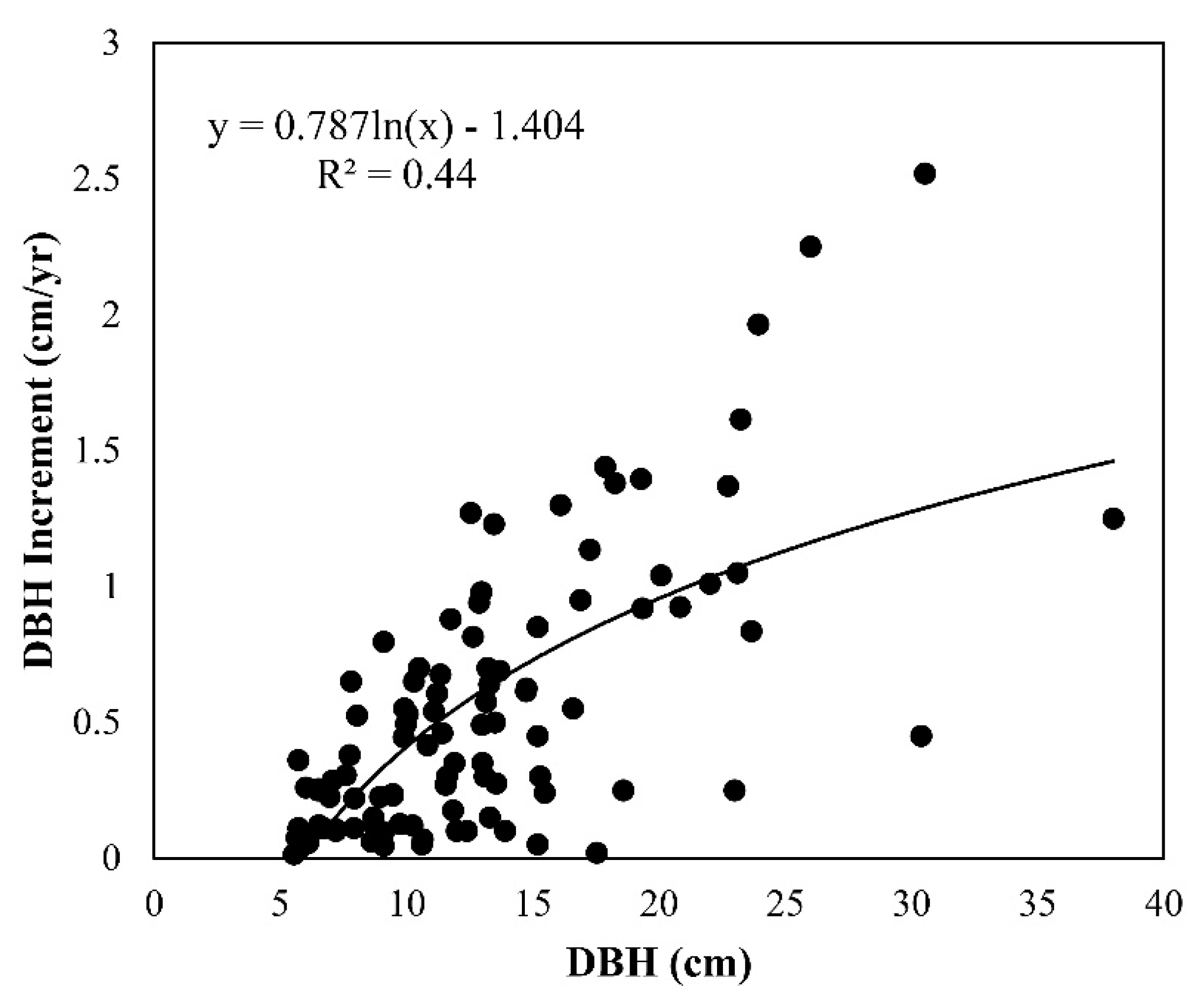
| Model | DBH Increment = 0.787ln(DBH) − 1.404 | |
|---|---|---|
| No of Samples (n) | 347 | |
| R | 0.67 | |
| R2 | 0.44 | |
| Constant | Variable Coefficients | |
| B | −1.404 | 0.787 |
| SE | 0.228 | 0.090 |
| t | −6.159 | 8.723 |
| Sig. | 0.000 * | 0.000 * |
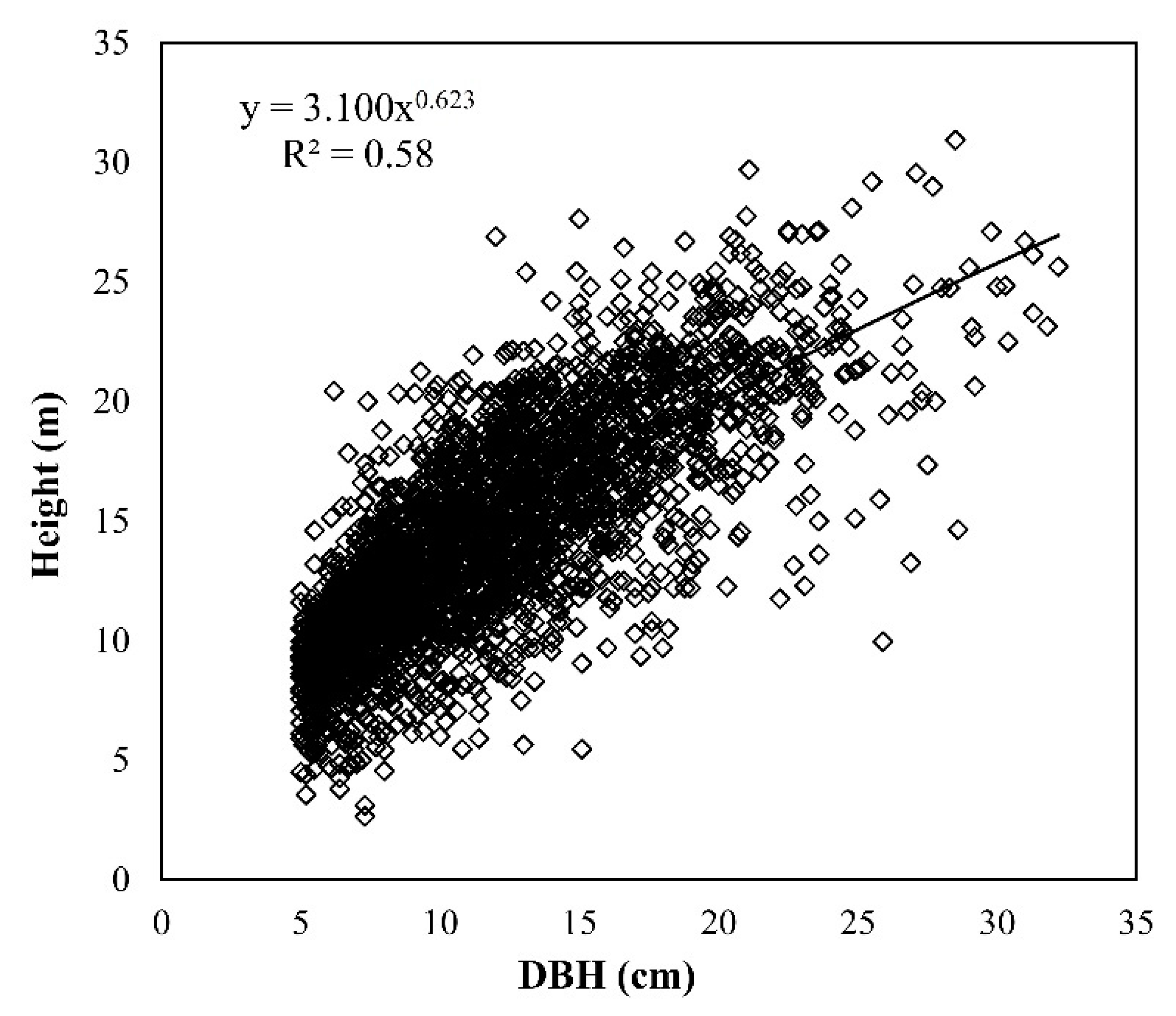
| Model | Height = 3.100(DBH)0.623 | |
|---|---|---|
| No of Samples (n) | 2760 | |
| R | 0.76 | |
| R2 | 0.58 | |
| Constant | Variable Coefficients | |
| B | 3.100 | 0.623 |
| SE | 0.075 | 0.010 |
| t | 41.176 | 61.991 |
| Sig. | 0.000 * | 0.000 * |
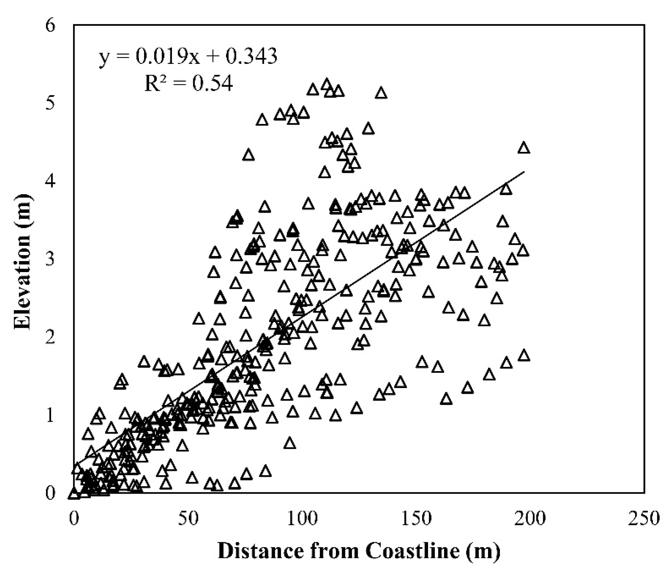
| Model | DTMmg = 0.019 (D) + 0.343 | |
|---|---|---|
| No of Samples (n) | 362 | |
| R | 0.73 | |
| R2 | 0.54 | |
| Constant | Variable Coefficients | |
| B | 0.343 | 0.019 |
| SE | 0.089 | 0.001 |
| t | 3.870 | 20.482 |
| Sig. | 0.000 * | 0.000 * |
| (a) 2000 | Groundtruths | Line Total | User’s Accuracy (%) | ||
| Mangrove | Non Mangrove | ||||
| Classification | Mangrove | 136 | 1 | 137 | 99.27 |
| Non Mangrove | 9 | 185 | 194 | 95.36 | |
| Column Total | 145 | 186 | 331 | ||
| Producer’s Accuracy (%) | 93.79 | 99.46 | |||
| Overall Accuracy = 96.98%; Overall Kappa = 0.94 | |||||
| (b) 2015 | Groundtruths | Line Total | User’s Accuracy (%) | ||
| Mangrove | Non Mangrove | ||||
| Classification | Mangrove | 114 | 4 | 118 | 96.61 |
| Non Mangrove | 16 | 195 | 211 | 92.42 | |
| Column Total | 130 | 199 | 329 | ||
| Producer’s Accuracy (%) | 87.69 | 97.99 | |||
| Overall Accuracy = 93.92%; Overall Kappa = 0.87 | |||||
| DBH (cm) | Height (m) | AGB (Mg ha−1) | ||
|---|---|---|---|---|
| Average | Observed | 11.89 | 14.30 | 196.88 |
| Estimated | 7.08 | 10.45 | 150.63 | |
| Minimum | Observed | 5.0 | 2.65 | 135.61 |
| Estimated | 5.95 | 9.41 | 138.52 | |
| Maximum | Observed | 49 | 30.95 | 291.31 |
| Estimated | 25.98 | 23.58 | 204.54 | |
| Standard Deviation | Observed | 5.44 | 4.43 | 32.58 |
| Estimated | 1.55 | 1.28 | 11.66 |
| Variables | R | R2 | Model Equation | RMSE Mg ha−1 | % RMSE | |
|---|---|---|---|---|---|---|
| Corrected | AGB – CHM | 0.76 | 0.57 | AGB = 2.51(CHM) + 128.28 | 8.59 | 5.70 |
| AGB – Ln CHM | 0.68 | 0.46 | AGB = 20.07(Ln CHM) + 108.24 | 9.36 | 6.21 | |
| Ln AGB – CHM | 0.77 | 0.60 | Ln AGB = 0.02(CHM) + 4.87 | 8.38 | 5.56 | |
| Uncorrected | AGB – CHM | 0.77 | 0.59 | AGB = 2.38(CHM) + 123.92 | 8.47 | 5.62 |
| AGB – Ln CHM | 0.69 | 0.47 | AGB = 23.78(Ln CHM) + 94.47 | 9.26 | 6.15 | |
| Ln AGB – CHM | 0.78 | 0.61 | Ln AGB = 0.01(CHM) + 4.85 | 8.24 | 5.47 |
© 2020 by the authors. Licensee MDPI, Basel, Switzerland. This article is an open access article distributed under the terms and conditions of the Creative Commons Attribution (CC BY) license (http://creativecommons.org/licenses/by/4.0/).
Share and Cite
Wong, C.J.; James, D.; Besar, N.A.; Kamlun, K.U.; Tangah, J.; Tsuyuki, S.; Phua, M.-H. Estimating Mangrove Above-Ground Biomass Loss Due to Deforestation in Malaysian Northern Borneo between 2000 and 2015 Using SRTM and Landsat Images. Forests 2020, 11, 1018. https://doi.org/10.3390/f11091018
Wong CJ, James D, Besar NA, Kamlun KU, Tangah J, Tsuyuki S, Phua M-H. Estimating Mangrove Above-Ground Biomass Loss Due to Deforestation in Malaysian Northern Borneo between 2000 and 2015 Using SRTM and Landsat Images. Forests. 2020; 11(9):1018. https://doi.org/10.3390/f11091018
Chicago/Turabian StyleWong, Charissa J., Daniel James, Normah A. Besar, Kamlisa U. Kamlun, Joseph Tangah, Satoshi Tsuyuki, and Mui-How Phua. 2020. "Estimating Mangrove Above-Ground Biomass Loss Due to Deforestation in Malaysian Northern Borneo between 2000 and 2015 Using SRTM and Landsat Images" Forests 11, no. 9: 1018. https://doi.org/10.3390/f11091018