Article

Identifying Variables to Discriminate between Conserved and Degraded Forest and to Quantify the Differences in Biomass

by
Yan Gao
1,*,
Margaret Skutsch
1,
Diana Laura Jiménez Rodríguez
2 and
Jonathan V. Solórzano
2
1
Centro de Investigaciones en Geografía Ambiental, Universidad Nacional Autónoma de México, Antigua Carretera a Pátzcuaro No. 8701, Col. Ex-Hacienda de San José de la Huerta, C.P. 58190 Morelia, Mexico
2
Posgrado en Geografía, Centro de Investigaciones en Geografía Ambiental, Universidad Nacional Autónoma de México, Antigua Carretera a Pátzcuaro No. 8701, Col. Ex-Hacienda de San José de la Huerta, C.P. 58190 Morelia, Mexico
*
Author to whom correspondence should be addressed.
Forests 2020, 11(9), 1020; https://doi.org/10.3390/f11091020
Submission received: 19 August 2020 / Revised: 4 September 2020 / Accepted: 17 September 2020 / Published: 22 September 2020

Abstract

:
The purpose of this work was to determine which structural variables present statistically significant differences between degraded and conserved tropical dry forest through a statistical study of forest survey data. The forest survey was carried out in a tropical dry forest in the watershed of the River Ayuquila, Jalisco state, Mexico between May and June of 2019, when data were collected in 36 plots of 500 m2. The sample was designed to include tropical dry forests in two conditions: degraded and conserved. In each plot, data collected included diameter at breast height, tree height, number of trees, number of branches, canopy cover, basal area, and aboveground biomass. Using the Wilcoxon signed-rank test, we show that there are significant differences in canopy cover, tree height, basal area, and aboveground biomass between degraded and conserved tropical dry forest. Among these structural variables, canopy cover and mean height separate conserved and degraded forests with the highest accuracy (both at 80.7%). We also tested which variables best correlate with aboveground biomass, with a view to determining how carbon loss in degraded forest can be quantified at a larger scale using remote sensing. We found that canopy cover, tree height, and density of trees all show good correlation with biomass and these variables could be used to estimate changes in biomass stocks in degraded forests. The results of our analysis will help to increase the accuracy in estimating aboveground biomass, contribute to the ongoing work on REDD+, and help to reduce the great uncertainty in estimation of emissions from forest degradation.

1. Introduction

Forest biomes provide important ecosystem services and habitat for many species [1] and sequester carbon through photosynthesis [2]. Forest degradation affects forest structure, function, ecosystem processes, and the capacity for carbon sequestration, generally also diminishing the provision of most ecosystem goods and services [3,4,5]. Unlike deforestation, there is no internationally accepted definition of forest degradation. Here, we adopt the definition from [6] that it is a human-induced disturbance in a forested landscape that results in carbon emissions but not a change in land cover. Forest degradation is usually a gradual process, which results in long-term damage while the forest remains in principle a forest. Forest degradation is often associated with anthropogenic activities, such as selective felling and cyclical use of forest, including shifting cultivation [7]. Cattle grazing causes forest degradation as a result of browsing on young tree shoots and trampling of soil. Fuelwood collection also causes low-intensity yet noticeable changes in forest structure. In many cases, these two latter activities cause small reductions of biomass below the forest canopy [6].
Tropical forests function as habitats for more than 45,000 tree species and store up to 66% of terrestrial biomass globally [8,9]. Nevertheless, tropical forests are under great pressure of deforestation and degradation, with more than 2000 km2 per year lost between 2000 and 2012 [10]. Although tropical forest loss is said to contribute 8%–15% of annual global anthropogenic carbon emissions to the atmosphere [11], neither the amount nor the locations of these contributions by forest degradation are clear. This uncertainty is due to factors related to lack of agreement in the definition of forest degradation and to the difficulties in monitoring forest degradation over extended areas [3,12]. There are more than 50 definitions for forest and forest degradation [13], and lack of clarity on ecological, anthropogenic, and conceptual aspects of forest degradation makes it difficult to select one that is universally applicable [14]. However, even if definitional issues are resolved, the mapping, monitoring, and quantification of forest degradation by remote sensing raise considerable challenges. Compared to deforestation, measuring, and monitoring of forest degradation requires much higher spatial resolution imagery to identify the more subtle changes typical of degradation activities [15]. Degraded forest forms a complex landscape often with mixed land cover, vegetation of different types and ages, dead trees, and bare soil patches, and because of the fast regrowth, the signature of the degradation often disappears within 1–2 years [3]; a typical case of this is the degradation caused by selective logging [16,17,18]. Moreover, while emissions from deforestation are usually calculated using an area estimate from remote sensing multiplied by an emission factor representing the average amount of carbon per hectare in each forest type, in the case of degradation, there is a need not only to estimate degraded areas but also to quantify the amount of carbon lost in any given forest in a particular year, which can vary enormously.
One method that has often been used to quantify forest degradation using remote sensing is by defining degradation as the gross change from primary forest to secondary forest, applying emission factors for “typical” secondary forest. This method is, however, flawed, because the classification of primary and secondary forest using remote sensing involves high uncertainties [19] and the error in the classified images will propagate into the results of change, making the quantification of forest degradation even more uncertain [20]. In addition, as mentioned already, the amounts of carbon lost in the conversion from primary forest to secondary forest are not in any way fixed or uniform. In order to obtain more accurate estimates of rates of degradation in the context of international policies, such as Reduced Emissions from Deforestation and forest Degradation (REDD+), a mixed method, involving both remote sensing and detailed ground-level forest surveys, will be necessary [21].
After disturbance, forests change their structural and compositional characteristics. A first step in developing mixed methods is therefore to establish to what extent degraded forest can be distinguished from conserved forest using ground level data. The purpose of this work was to determine which structural variables present statistically significant differences between degraded and conserved tropical dry forests. When this is clear, the capacity of remotely sensed data to pick up these variables can be tested. This paper is a first step towards developing a methodology linking ground characteristics with remote sensing, since it will tell us which characteristics are the most relevant at ground level to distinguish between conserved and degraded forest and which can be used to estimate the changing biomass levels within degraded forest, allowing estimation of emissions due to degradation.
Carbon emissions can most easily and accurately be calculated directly from changes in aboveground biomass (AGB) from year to year, on the assumption that approximately 50% of dry biomass consists of carbon [22]. AGB is defined as the mass of above ground living organic material in a given area [22] and it is a variable that is derived from estimates of dimensions of trees, such as basal area. Quantification of basal area, however, requires physical measurement of tree diameters (i.e., diameter at breast height) in the field, and changes in the basal area over time would require repeated surveys, which would be prohibitively expensive to carry out in most situations because it is highly labor intensive. Hence, the question arises of whether other variables, data on which could be acquired with less effort, could be used as proxies. Canopy cover, for example, has been assessed using medium- to high-resolution remote sensing platforms, such as Landsat [23,24], Sentinel-1 [25], and Sentinel-2 [26]. High spatial resolution canopy height models could be derived using images, such as GeoEye and Worldview-3 combined with a digital elevation model [27], and density of trees could potentially be obtained from photos taken from drones [28,29]. If such variables correlate strongly with AGB, then they could substitute for physical measurements of tree diameters in the calculation of emissions.

2. Materials and Methods

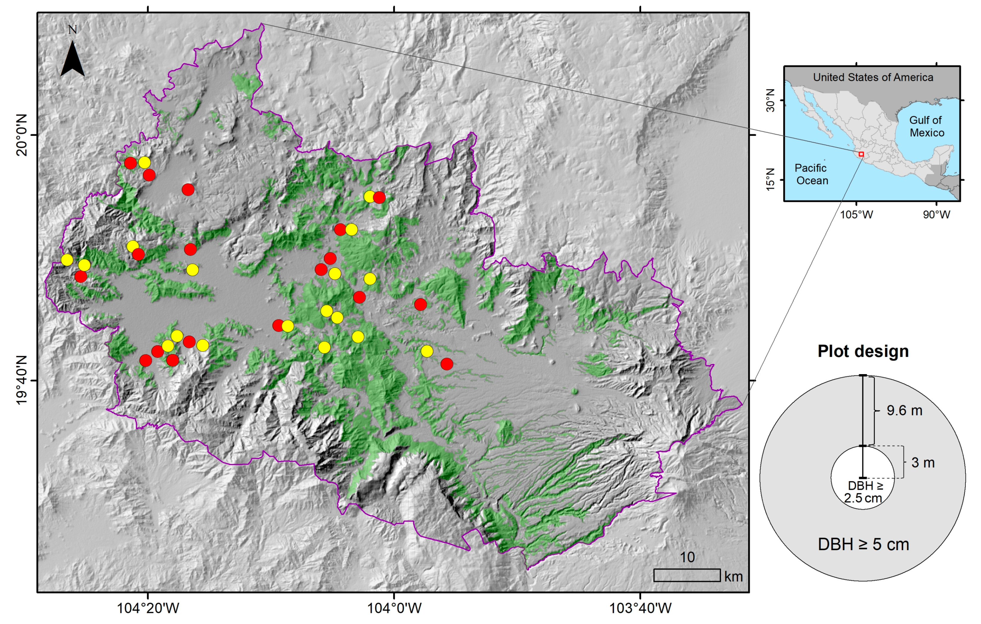
2.1. Study Focus and Area: Degradation in Forests of the Watershed of the Ayuquila River

The study area is located in the western Pacific area of Mexico, in the watershed of the Ayuquila River (Figure 1). Its topography ranges from 260 to 2500 m above mean seal level; the average annual precipitation is 800–1200 mm and occurs mostly between June and October; the average monthly temperature ranges from 18 to 22 °C [30]. Tropical dry forest (TDF) is distributed in the lower topographic areas. It is composed of deciduous and semi-deciduous woodlands with low biomass density, canopy height, and cover, and has low AGB compared to other areas of TDFs in the Neotropics [31]. TDFs in Mexico are widespread and they suffer higher rates of forest loss compared to the humid tropical forests due to higher population densities [32]. TDF in Ayuquila watershed is heavily used for shifting cultivation, fuelwood extraction, cattle grazing, extraction of poles for constructing fences, and for mushrooms and medicinal plants [33]. As in the rest of Mexico, most of the forests in the Ayuquila watershed are under the authority of ejidos, which are communally managed rural agrarian settlements [33]. The Mexican government created ejido in the 1930s as a type of community landholding for small-scale subsistence-based agriculture [34,35]. Across Mexico, about 52% of all land and 55% of all forestlands are in the hands of ejidos [36].
There are both permanent and shifting cultivation agriculture systems in the Ayuquila area. Permanent agriculture, which is under rain-fed and irrigated farming systems, is distributed over the lower elevations and flat areas, which have been completely cleared of TDF in the past 20–30 years [37], while areas of shifting cultivation are distributed within existing TDF in a mosaic landscape, which changes from year to year, as cultivated areas are left fallow and secondary forest regrows. Shifting cultivation is the main driver of forest degradation in the TDF in this area, although cattle grazing, fuelwood extraction, and extraction of poles for fences are contributory causes [38].

2.2. Sampling Design

For our analysis, we started with a recent land cover map (2018) to identify all patches in the study area that were covered by tropical dry forest at the time of our study. We then used Google Earth Pro, comparing images from 2016–2018 to identify patches of tropical dry forest where there had been visible changes in the texture between these dates. We randomly selected 30 points in areas where change had evidently occurred (i.e., where forest had clearly been degraded) and 30 in areas that had not changed (representing conserved forest). We then considered the accessibility of the sampling points following the criteria that the sampling points should not be further than 3000 m from principal roads and should have slopes of less than 30 degrees (for practical reasons). We also checked these 60 sample locations with the Junta Intermunicipal del Río Ayuquila (JIRA), a local environmental non-governmental organization (NGO), regarding security. As a result of these two filters, we excluded 5 of the plots identified in conserved forests and 12 of the plots in degraded forests, leaving 43 potential sampling sites, of which 25 were in conserved forest and 18 in degraded. In order to balance the sampling design, we eliminated at random 7 plots from the conserved forest group.

2.3. Forest Survey Data Collection

The field survey was carried out between May and June 2019, which is at the end of the dry season and the beginning of the rainy season. The field data were collected in 36 plots of 500 m2 each. As explained above, of the total 36 plots, 18 were in conserved and 18 in degraded forest.
In each plot, data were collected on diameter at breast height (DBH), tree height, number of branches, canopy cover, and number of trees per plot, from which basal area, AGB, and density of trees per hectare were calculated. All trees with DBH greater than 2.5 cm were measured in a radius of 3 m from the center of the plot, and all individuals with DBH greater than 5 cm were measured up to a radius of 12.6 m (Figure 1). Canopy cover was measured as the percentage of a spherical densometer grid covered by forest canopy. In addition, the presence of anthropogenic activities, such as cattle and cattle feces, logged tree trunks, leaves, and seedlings, was noted, as this supported identification of plots as being “degraded”.

2.4. AGB and Basal Area

AGB data was calculated using the allometric Equation (1) developed by Martínez-Yrizar et al. [39]:
l o g 10   A G B = A +   l o g 10   B A .
This equation is adjusted to tropical dry forests, where A G B is in kg/m2, A is the regression constant—here, we adopt the value—0.5352—and B A is the basal area in cm2.
Basal area was calculated from the following formula (Equation (2)) using the diameter at breast height ( D B H ):
B A =   π ( D B H 2 ) 2

2.5. Statistical Methods

The study assumes that variables that are found from ground level data to be statistically different between degraded and conserved forest can potentially be modelled using spectral information. The values of the structural variables in forests of conserved and degraded status were first analyzed by computing statistics, such as the maximum, minimum, mean, and standard deviation. Since the distributions of the forest structure variables were found to violate the assumption of normality [40], we applied the Wilcoxon signed-rank test, the non-parametric version of a paired samples t-test, to check which variables were significantly different between degraded and conserved forest. The null hypothesis was that the mean value of the structural variables would be the same in degraded and conserved forests.
Afterwards, we tested which structural variables discriminate well between the two types of forest. We fitted six binomial logistic regressions in which each model included a single structural variable as the independent variable and the forest condition (conserved vs. degraded) as the dependent variable. Using these models, the threshold value was determined to separate degraded and conserved forest with a 50% probability for each structural variable. We predicted forest types according to these logistic regressions and computed the overall accuracy for each model as the proportion of correctly classified plots over the total number of plots. The complete set of plots was used to fit the model as well as to evaluate the accuracy.
Finally, we explored the correlation between the structural variables, first with forest types combined and then separately. Special emphasis was placed on identifying attribute variables that have a significant correlation with AGB. If these variables can be quantified with remote sensing sensors, they could be used to assess AGB and estimate emissions from forest degradation.
All the statistical data analysis including Wilcoxon signed-rank test, logistic regression, classification, and Kendall’s correlation, was carried out in R [41]. The data and the scripts can be accessed from https://github.com/JonathanVSV/Conserved-vs-Degraded-Forest.

3. Results

3.1. How Well Can the Structural Variables Differentiate These Two States of Forest?

We first evaluated whether the values of forest structural variables differ between the two types of forest (i.e., conserved and degraded). The structural parameters measured are summarized in Table 1.
Looking at the data in Table 1, it appears that the variable that is most commonly used in remote sensing to distinguish degraded from conserved forest—canopy cover—is not necessarily a good indicator, since although the mean value is undoubtedly lower in degraded forests, there is considerable overlap at the top end, and the same is true for tree height. We note that because of the way TDF regrows (particularly after shifting cultivation), forests classified as degraded tend to have more individual trees with more branches than conserved forests, despite the fact that they have much lower basal area and AGB. In other words, most of the degraded forests are in fact recovering, and have larger numbers of thinner more branching trees than conserved forest, presumably because light conditions following clearance support the production of large numbers of saplings. Since none of the forest structural variables followed a normal distribution, we applied the non-parametric Wilcoxon signed-rank test to determine if the differences in their mean values could be considered significant. We found statistically significant differences between the mean values of four of the six variables: canopy cover, basal area, height, and biomass. As for density of trees and branches, they are not significantly different between degraded and conserved forests (Table 2).
Figure 2 identifies the structural variables that significantly differ between the two forest conditions. As can be seen, conserved forests show statistically higher values for canopy cover, tree height, and basal area. Since AGB is directly calculated from basal area, this variable obviously also differs between conserved and degraded forest. Importantly, we also note that although there can be overlap between the maximum canopy cover (100%) of conserved and degraded forest (Table 1), in practice only a limited number of plots (2 in 18 plots of conserved forests, and 5 in 18 plots of degraded forests) present this overlap; the mean values are statistically different and the standard deviations sufficiently small, in theory, for these two classes to be distinguished. As expected, the logistic regression models showed a significant coefficient (β) for canopy cover (z = −2.41, p = 0.02), basal area (z = −2.60, p = 0.01), mean height (z = −2.75, p = 0.01), and AGB (z = −2.60, p = 0.01) as explanatory variables to classify the plots into degraded and conserved forests, while the models that used density of branches (z = 0.93, p = 0.35) and density of trees did not (z = −0.18, p = 0.86). Using these models, we found the threshold values to separate the degraded and conserved forests for the four variables as the following: canopy cover: 90.9%; basal area: 9.45 m2/ha; height: 5.30 m; and AGB: 27.5 Mg/ha.
The overall accuracies obtained using these logistic regression models were canopy cover 80.56%, basal area 72.22%, mean height 80.56, and AGB 72.22%. Basal area and AGB are not independent variables, and thus, it is not surprising that they show the same accuracy when used to classify the plots into degraded and conserved forest. It became evident that the two statuses of forests showed an overlap in each of the quantified structural variables (Figure 2). Canopy cover and mean height appear to be the most promising structural variables for classifying forests into degraded and conserved conditions, partially because of the very low variance on these variables in conserved forests.

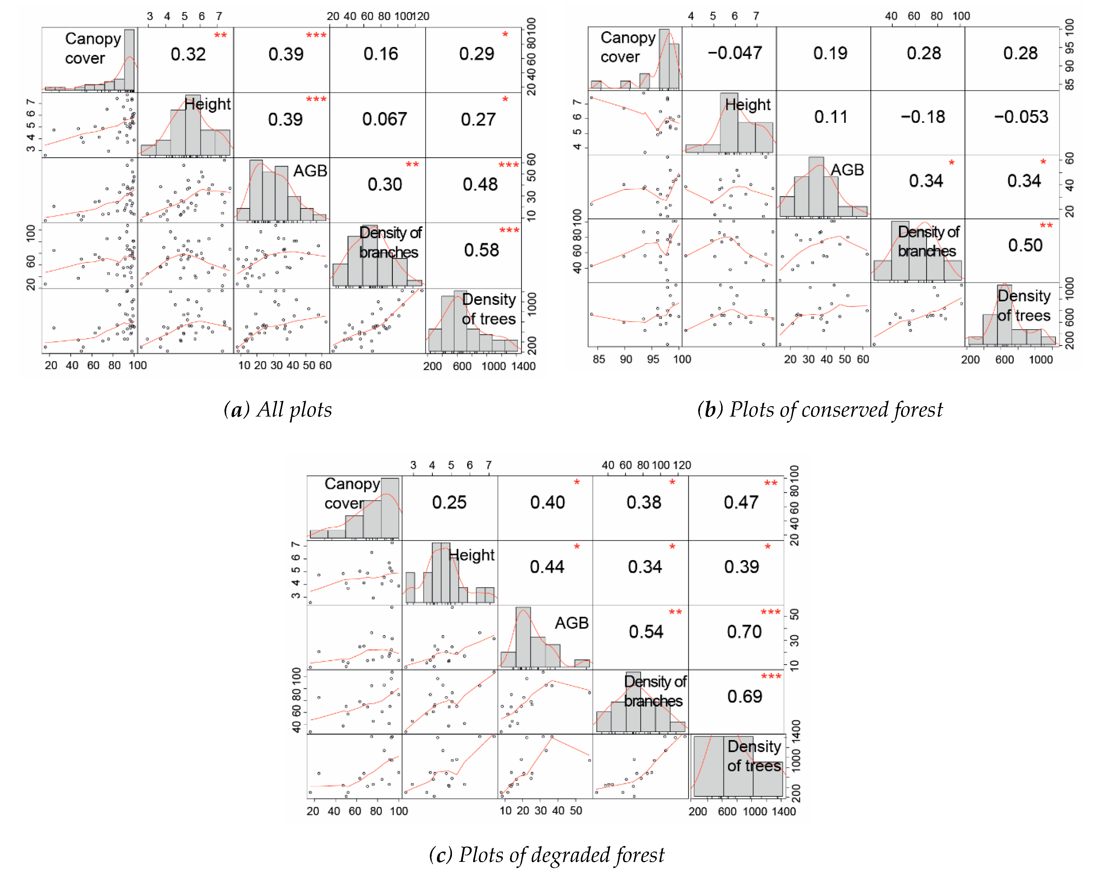
3.2. Correlation between Variables of Forest Attributes

Inter-correlations at plot level were calculated for all the forest structural variables except basal area, since basal area and biomass have a 100% correlation. The primary purpose of this analysis was to see to what extent the variables that can be measured using remote sensing methods—particularly canopy cover, density of trees, and tree height—might be used to predict variables, which, if measured over time, would reflect changes in AGB, and which could then be used to estimate emissions due to degradation. The Kendall tau correlation was applied, and the results are shown in Figure 3.
When all plots are taken together (Figure 3a), we see that AGB is correlated with canopy cover, tree height, and density of trees, at a high level of statistical significance (τ = 0.39, τ = 0.39, and τ = 0.48, respectively, at p < 0.001). AGB is also correlated with density of branches, although with a lower significance coefficient (τ = 0.30, p < 0.01). Canopy cover is correlated with density of trees and tree height, although there is no correlation between canopy cover and density of branches. Density of trees and density of branches are also highly correlated (τ = 0.58, p < 0.001). For the case of conserved forest (Figure 3b), AGB is only correlated with density of trees and density of branches (both at τ = 0.34, p < 0.05). However, in degraded forest (Figure 3c) there is a very good correlation between AGB and density of trees (τ = 0.7, p < 0.001). There is also good correlation between AGB and density of branches (τ = 0.54, p < 0.05), canopy cover (τ = 0.4, p < 0.05), and tree height (τ = 0.44, p < 0.01). In addition, there is good correlation between density of trees and canopy cover (τ = 0.47, p < 0.01) and between density of trees and tree height (τ = 0.39, p < 0.05). Density of branches and tree height (τ = 0.34, p < 0.05), density of branches and canopy cover (τ = 0.38, p < 0.05), and density of trees and density of branches (τ = 0.69, p < 0.001) are all significantly correlated in degraded forest. However, canopy cover and tree height is not correlated.

4. Discussion

In the context of programs such as REDD+, it is loss and gain of biomass that is the primary variable of concern, since it is from this that the flux of carbon can be calculated. The analysis shows that several forest attributes that are regularly recorded in forest surveys could be used to distinguish degraded and conserved forests at ground level. These variables include mean canopy cover and mean tree height, basal areas, and AGB. The analysis also shows that the density of trees and density of branches do not significantly differ between these two states of forest. We observed that the variance of all variables is much higher in the degraded plots than in the conserved plots, indicating greater variability in the degraded forest. This is entirely to be expected, since these forests are in a state of constant change following human disturbances. This finding strongly underlines the importance of not using a standard default value for carbon stocks in degraded forest and the need for much more careful assessment of changes in the level of carbon stocks in degraded forest over time.
Applying the threshold obtained by the logistic model to classify the plots into degraded and conserved states, canopy cover and mean height are the variables that enable the highest accuracy (-both at 80.56%). This makes canopy cover and mean height the most suitable indicators of forest status. Although mean canopy cover in theory discriminates reasonably well between conserved and degraded forest, this variable has a wide standard deviation in degraded forest, with one plot of degraded forest having 100% canopy cover, which means that it would be misclassified if only this criterion were used, although the mean value of canopy cover of all plots of degraded forest was much lower, and the standard deviations do not overlap (Figure 2). In the case of mean height, the two types of forest can also be discriminated, with a small fraction of plots wrongly classified using the threshold value. However, it is expected that if two or more variables were to be combined, the error in the discrimination of conserved and degraded forest would be reduced, enabling a much more definitive separation between conserved and degraded forest. Nevertheless, these results also suggest that, based only on structural variables from field measurements, these two types of forest can only be distinguished up to a certain degree.
In terms of the correlations between structural variables and AGB, we find that when both types of forest are analyzed together, density of trees has the highest correlation with AGB (τ = 0.48, p < 0.001), followed by canopy cover and canopy height (both at τ = 0.31, p < 0.01). In plots of only conserved forest, AGB is only correlated with density of trees and density of branches. In plots of only degraded forest, both density of trees (τ = 0.70, p < 0.001) and canopy cover (τ = 0.40, p < 0.05) appear to be correlated with AGB. A possible limitation of our study, however, was that we made a distinction between “conserved” and “degraded” forests. A more nuanced classification of forest into several levels of degradation (i.e., highly degraded, moderately degraded, and lightly degraded) might have produced better results in terms of variables to predict AGB.
Both canopy cover and canopy (tree) height are correlated with AGB both for forest in general (both forest types analyzed together), and for degraded forest only, while for conserved forest, these two attribute variables do not show significant correlation with AGB. Canopy cover is the most easily and commonly measured variable when using optical remote sensing of medium to high spatial resolution satellite imagery [42,43], also when using Light Detection and Ranging (LiDAR) data [26,44], although this last can also be used to estimate canopy height [45,46,47,48,49,50]. Density of trees is also a reasonably good predictor of AGB in both conserved and degraded forest (with more, though thinner, trees in degraded forest), but density of trees cannot be detected with low or medium spatial resolution optical imagery. Such data could, however, be obtained via aerial photographs or very high spatial resolution imagery or LiDAR borne on drones [51,52,53]. Although most of the published work has been for temperate forest in northern Europe, Canada, or USA, few experiments have been reported for tropical forest, probably due to the complicity of the composition and seasonality. Possibly an index that combines tree height and density of trees measured from a drone or airborne LiDAR could be developed as a predictor of AGB in degraded TDF. It would certainly be worth exploring the potential of such an index for assessing changing carbon stock in degraded forest where significant changes are expected.
LiDAR estimates of AGB have been shown to be highly correlated with field-measured AGB data. For example, Hernandez-Stefanoni et al. [32] show a high association between AGB and LiDAR data with an R2 = 0.87 using a linear regression analysis. An advantage of LiDAR data is that they do not get saturated in areas of high biomass; however, the high cost of acquisition could be a limitation [6]. It is worth noting that the Global Ecosystem Dimension Investigacion (GEDI) LiDAR mission (https://gedi.umd.edu/mission/mission-overview/), launched in December 2018, makes accurate measurements of canopy height, vertical canopy structure, and surface elevation and shows promise in improving measurements of AGB and forest carbon [54]. Synthetic aperture radar (SAR) data have also shown potential in biomass estimation. In particular, more accurate results have been found with longer wavelengths, such as L-band (23 cm wavelength) SAR [55]. L-band SAR has been used to estimate biomass in forest areas with low biomass [56,57]. In addition, the BIOMASS sensor from the European Satellite Agency (ESA), to be launched in 2022, will collect data at the P-band (70 cm wavelength) wavelength. It has potential to see through leafy treetops to build up maps of tree height and volume, and therefore it is expected to provide precise information on global forest biomass and carbon content and fill the gap of forest biomass density monitoring [58]. Since the data from L-band and P-band SAR become saturated in forest with a medium to high biomass level at approximately 60–100 and 100–150 Mg ha−1, respectively, they are not suitable for mapping forest biomass in all conditions [55,59], although they should function well at the densities we found in degraded forests in Ayuquila River watershed.. The application of texture data derived from L-band SAR has been reported to be able to reduce the saturation at high biomass values, since texture data capture variation in horizontal forest structure attributes, such as tree height and crown diameter [32]. The best result could probably be obtained with a combination of optical, LiDAR, and SAR data [60].

5. Conclusions

This paper presented findings of a statistical study of conserved and degraded forests based on a recent forest survey in TDF. The forest attributes that are significantly different between conserved and degraded forests include canopy cover, basal area, tree height, and AGB. Although canopy cover presents large variance in degraded forests, there is large difference in mean AGB between degraded and conserved forest. Among the four variables, canopy cover and canopy (tree) height separate degraded and conserved forests with the least error, which makes these two variables the most suitable to discriminate these two forest conditions. In terms of variables that could be used to estimate biomass stocks in degraded forests, density of trees, canopy cover, and canopy (tree) height all show a good correlation with AGB. It is clear that for accurate estimation of emissions from degraded forest, very high spatial resolution satellite images, including drone-based imaging LiDAR and radar data, are essential. An important next step would be to calibrate canopy cover, canopy height, or density of trees against degradation using a sliding scale of intensity of degradation as observed at ground level. This would likely enable a more reliable estimation of area of degradation and quantification of AGB using remote sensing.

Author Contributions

Y.G. and D.L.J.R. conceived and designed the experiments; Y.G. and D.L.J.R. performed the experiment; Y.G., D.L.J.R. and J.V.S. analyzed the data; D.L.J.R. and J.V.S. contributed analysis tools; Y.G. and M.S. wrote the paper. All authors have read and agreed to the published version of the manuscript.

Funding

This research was supported financially by the Consejo Nacional de Ciencia y Tecnología (CONACYT) grant number ‘Ciencia Básica’ SEP-285349.

Acknowledgments

The authors would like to acknowledge Jaime Octavio Loya Carrillo, Ernesto Carrillo, Miriam San Jose, Rita Adame, and Miguel Salinas for their assistance and participation in the data collection. Thanks also go to Samuel and Oscar Ponce from JIRA for their valuable advice during the fieldwork.

Conflicts of Interest

The authors declare no conflict of interest.

References

  1. Gentry, A. Tropical Forest Biodiversity—Distributional Patterns and their Conservational Significance. OIKOS 1992, 63, 19–28. [Google Scholar] [CrossRef]
  2. Buettel, J.C.; Ondei, S.; Brook, B.W. Missing the wood for the trees? New ideas on defining forests and forest degradation. Rethink. Ecol. 2017, 1, 15–24. [Google Scholar] [CrossRef]
  3. Herold, M.; Román-Cuesta, R.M.; Mollicone, D.; Hirata, Y.; Van Laake, P.; Asner, G.P.; Souza, C.; Skutsch, M.; Avitabile, V.; MacDicken, K. Options for monitoring and estimating historical carbon emissions from forest degradation in the context of REDD+. Carbon Balance Manag. 2011, 6, 13. [Google Scholar] [CrossRef] [PubMed] [Green Version]
  4. Chazdon, R.L.; Brancalion, P.H.S.; Laestadius, L.; Bennett-Curry, A.; Buckingham, K.; Kumar, C.; Moll-Rocek, J.; Vieira, I.C.G.; Wilson, S.J. When is a forest a forest? Forest concepts and definitions in the era of forest and landscape restoration. Ambio 2016, 45, 538–550. [Google Scholar] [CrossRef]
  5. Modica, G.; Merlino, A.; Solano, F.; Mercurio, R. An index for the assessment of degraded Mediterranean forest ecosystems. For. Syst. 2015, 24, 5. [Google Scholar] [CrossRef] [Green Version]
  6. GFOI. Integration of Remote-Sensing and Ground-Based Observations for Estimation of Emissions and Removals of Greenhouse Gases in Forests: Methods and Guidance from the Global Forest Observations Initiative; Food and Agriculture Organization: Rome, Italy, 2016. [Google Scholar]
  7. Thompson, I.D.; Guariguata, M.R.; Okabe, K.; Bahamondez, C.; Nasi, R.; Heymell, V.; Sabogal, C. An operational framework for defining and monitoring forest degradatio. Ecol. Soc. 2013, 18. [Google Scholar] [CrossRef]
  8. Slik, J.W.F.; Arroyo-Rodríguez, V.; Aiba, S.I.; Alvarez-Loayza, P.; Alves, L.F.; Ashton, P.; Balvanera, P.; Bastian, M.L.; Bellingham, P.J.; van den Berg, E.; et al. An estimate of the number of tropical tree species. Proc. Natl. Acad. Sci. USA 2015, 112, 7472–7477. [Google Scholar] [CrossRef] [Green Version]
  9. Pan, Y.; Birdsey, R.A.; Phillips, O.L.; Jackson, R.B. The Structure, Distribution, and Biomass of the World’s Forests. Annu. Rev. Ecol. Evol. Syst. 2013, 44, 593–622. [Google Scholar] [CrossRef] [Green Version]
  10. Hansen, M.C.; Potapov, P.V.; Moore, R.; Hancher, M.; Turubanova, S.A.; Tyukavina, A.; Thau, D.; Stehman, S.V.; Goetz, S.J.; Loveland, T.R.; et al. High-Resolution Global Maps of 21st-Century Forest Cover Change. Science 2013, 342, 850–853. [Google Scholar] [CrossRef] [Green Version]
  11. Houghton, R.A.; Byers, B.; Nassikas, A.A. A role for tropical forests in stabilizing atmospheric CO2. Nat. Clim. Chang. 2015, 5, 1022–1023. [Google Scholar] [CrossRef]
  12. Bullock, E.L.; Woodcock, C.E.; Olofsson, P. Monitoring tropical forest degradation using spectral unmixing and Landsat time series analysis. Remote Sens. Environ. 2020, 238, 110–968. [Google Scholar] [CrossRef]
  13. Putz, F.E.; Redford, K.H. The Importance of Defining’Forest’: Tropical Forest Degradation, Deforestation, Long-term Phase Shifts, and Further Transitions. Biotropica 2010, 42, 10–20. [Google Scholar] [CrossRef]
  14. Ghazoul, J.; Burivalova, Z.; Garcia-Ulloa, J.; King, L.A. Conceptualizing Forest Degradation. Trends Ecol. Evol. 2015, 30, 622–632. [Google Scholar] [CrossRef] [PubMed]
  15. Pearson, T.R.H.; Brown, S.; Murray, L.; Sidman, G. Greenhouse gas emissions from tropical forest degradation: An underestimated source. Carbon Balance Manag. 2017, 12, 3. [Google Scholar] [CrossRef] [Green Version]
  16. Asner, G.P.; Heidebrecht, K.B. Spectral unmixing of vegetation, soil and dry carbon cover in arid regions: Comparing multispectral and hyperspectral observations. Int. J. Remote Sens. 2002, 23, 3939–3958. [Google Scholar] [CrossRef]
  17. Souza, A.F.; Martins, F.R. Spatial variation and dynamics of flooding, canopy openness, and structure in a Neotropical swamp forest. Plant Ecol. 2005, 180, 161–173. [Google Scholar] [CrossRef]
  18. Stone, T.A.; Lefebvre, P. Using multi-temporal satellite data to evaluate selective logging in Para, Brazil. Int. J. Remote Sens. 1998, 19, 2517–2526. [Google Scholar] [CrossRef]
  19. INEGYCEI. Inventario Nacional de Emisiones de Gases y Compuestos de Efecto Invernadero 1990–2015; Secretaría de Medio Ambiente y Recursos Naturales and Instituto Nacional de Ecología y Cambio Climático: Ciudad de México, Mexico, 2018. [Google Scholar]
  20. Pelletier, J.; Kirby, K.R.; Potvin, C. Significance of carbon stock uncertainties on emission reductions from deforestation and forest degradation in developing countries. For. Policy Econ. 2012, 24, 3–11. [Google Scholar] [CrossRef]
  21. Gao, Y.; Skutsch, M.; Paneque-Gálvez, J.; Ghilardi, A. Remote sensing of forest degradation: A review. Environ. Res. Lett. 2020. [Google Scholar] [CrossRef]
  22. Karjalainen, T.; Richards, G.; Hernandez, T.; Kainja, S.; Lawson, G.; Liu, S.; Pardo, J.I.A.; Birdsey, R.; Boehm, M.; Daka, J.; et al. IPCC Report on Definitions and Methodological Options to Inventory Emissions from Direct Human-induced Degradation of Forests and Devegetation of Other Vegetation Types; Intergovernmental Panel on Climate Change: Kanagawa, Japan, 2003; p. 30. [Google Scholar]
  23. Vogeler, J.C.; Braaten, J.D.; Slesak, R.A.; Falkowski, M.J. Extracting the full value of the Landsat archive: Inter-sensor harmonization for the mapping of Minnesota forest canopy cover (1973–2015). Remote Sens. Environ. 2018, 209, 363–374. [Google Scholar] [CrossRef]
  24. Baumann, M.; Levers, C.; Macchi, L.; Bluhm, H.; Waske, B.; Gasparri, N.I.; Kuemmerle, T. Mapping continuous fields of tree and shrub cover across the Gran Chaco using Landsat 8 and Sentinel-1 data. Remote Sens. Environ. 2018, 216, 201–211. [Google Scholar] [CrossRef]
  25. Zhang, W.; Brandt, M.; Wang, Q.; Prishchepov, A.V.; Tucker, C.J.; Li, Y.; Lyu, H.; Fensholt, R. From woody cover to woody canopies: How Sentinel-1 and Sentinel-2 data advance the mapping of woody plants in savannas. Remote Sens. Environ. 2019, 234, 111–465. [Google Scholar] [CrossRef]
  26. Korhonen, L.; Hadi; Packalen, P.; Rautiainen, M. Comparison of Sentinel-2 and Landsat 8 in the estimation of boreal forest canopy cover and leaf area index. Remote Sens. Environ. 2017, 195, 259–274. [Google Scholar] [CrossRef]
  27. Meddens, A.J.H.; Vierling, L.A.; Eitel, J.U.H.; Jennewein, J.S.; White, J.C.; Wulder, M.A. Developing 5 m resolution canopy height and digital terrain models from WorldView and ArcticDEM data. Remote Sens. Environ. 2018, 218, 174–188. [Google Scholar] [CrossRef]
  28. Mohan, M.; Silva, C.A.; Klauberg, C.; Jat, P.; Catts, G.; Cardil, A.; Hudak, A.T.; Dia, M. Individual Tree Detection from Unmanned Aerial Vehicle (UAV) Derived Canopy Height Model in an Open Canopy Mixed Conifer Forest. Forests 2017, 8, 340. [Google Scholar] [CrossRef] [Green Version]
  29. Zhang, J.; Hu, J.; Lian, J.; Fan, Z.; Ouyang, X.; Ye, W. Seeing the forest from drones: Testing the potential of lightweight drones as a tool for long-term forest monitoring. Biol. Conserv. 2016, 198, 60–69. [Google Scholar] [CrossRef]
  30. Cuevas, R.; Nuñez, N.M.; Guzman, F.; Santana, M. El bosque tropical caducifolio en la reserva de la Biosfera Sierra Manantlan, Jalisco-Colima, Mexico. Bol. IBUG 1998, 5, 445–491. [Google Scholar]
  31. Becknell, J.M.; Kissing Kucek, L.; Powers, J.S. Aboveground biomass in mature and secondary seasonally dry tropical forests: A literature review and global synthesis. For. Ecol. Manag. 2012, 276, 88–95. [Google Scholar] [CrossRef]
  32. Hernández-Stefanoni, J.L.; Castillo-Santiago, M.Á.; Mas, J.F.; Wheeler, C.E.; Andres-Mauricio, J.; Tun-Dzul, F.; George-Chacón, S.P.; Reyes-Palomeque, G.; Castellanos-Basto, B.; Vaca, R.; et al. Improving aboveground biomass maps of tropical dry forests by integrating LiDAR, ALOS PALSAR, climate and field data. Carbon Balance Manag. 2020, 15, 15. [Google Scholar] [CrossRef]
  33. Borrego, A.; Skutsch, M. Estimating the opportunity costs of activities that cause degradation in tropical dry forest: Implications for REDD+. Ecol. Econ. 2014, 101, 1–9. [Google Scholar] [CrossRef]
  34. Barnes, G. The evolution and resilience of community-based land tenure in rural Mexico. Land Use Policy 2009, 26, 393–400. [Google Scholar] [CrossRef]
  35. Perramond, E.P. The Rise, Fall, and Reconfiguration of the Mexican “Ejido”. Geogr. Rev. 2008, 98, 356–371. [Google Scholar] [CrossRef]
  36. Madrid, L.; Núñez, J.M.; Quiroz, G. La propiedad social forestal en México. Investig. Ambient. 2009, 1, 179–196. [Google Scholar]
  37. Morales-Barquero, L.; Skutsch, M.; Jardel-Peláez, E.J.; Ghilardi, A.; Kleinn, C.; Healey, J.R. Operationalizing the definition of forest degradation for REDD+, with application to Mexico. Forests 2014, 5, 1653–1681. [Google Scholar] [CrossRef] [Green Version]
  38. Morales-Barquero, L. Beyond Carbon Accounting: A Landscape Perspective on Measuring and Monitoring Tropical Forest Degradation. Ph.D. Thesis, Bangor University, Bangor, Maine, 2016. [Google Scholar]
  39. Martinez-Yrizar, A.; Sarukhan, J.; Perez-Jimenez, A.; Rincon, E.; Maass, J.M.; Solis-Magallanes, A.; Cervantes, L. Above-ground phytomass of a tropical deciduous forest on the coast of Jalisco, México. J. Trop. Ecol. 1992, 8, 87–96. [Google Scholar] [CrossRef] [Green Version]
  40. Hollander, M.; Wolfe, D.A.; Chicken, E. Nonparametric Statistical Methods; Wiley Series in Probability and Statistics; John Wiley & Sons, Inc.: New York, NY, USA, 1999; ISBN 978-0-470-38737-5. [Google Scholar]
  41. R Core Team. R: A Language and Environment for Statistical Computing; R Foundation for Statistical Computing: Vienna, Austria, 2020. [Google Scholar]
  42. Potapov, P.V.; Turubanova, S.A.; Hansen, M.C.; Adusei, B.; Broich, M.; Altstatt, A.; Mane, L.; Justice, C.O. Quantifying forest cover loss in Democratic Republic of the Congo, 2000–2010, with Landsat ETM+ data. Remote Sens. Environ. 2012, 122, 106–116. [Google Scholar] [CrossRef]
  43. Chopping, M.; Su, L.; Rango, A.; Martonchik, J.V.; Peters, D.P.C.; Laliberte, A. Remote sensing of woody shrub cover in desert grasslands using MISR with a geometric-optical canopy reflectance model. Remote Sens. Environ. 2008, 112, 19–34. [Google Scholar] [CrossRef]
  44. Korhonen, L.; Korpela, I.; Heiskanen, J.; Maltamo, M. Airborne discrete-return LIDAR data in the estimation of vertical canopy cover, angular canopy closure and leaf area index. Remote Sens. Environ. 2011, 115, 1065–1080. [Google Scholar] [CrossRef]
  45. Ahmed, O.S.; Franklin, S.E.; Wulder, M.A. Integration of Lidar and Landsat Data to Estimate Forest Canopy Cover in Coastal British Columbia. Photogramm. Eng. Remote Sens. 2014, 80, 953–961. [Google Scholar] [CrossRef] [Green Version]
  46. Ahmed, O.S.; Franklin, S.E.; Wulder, M.A.; White, J.C. Characterizing stand-level forest canopy cover and height using Landsat time series, samples of airborne LiDAR, and the Random Forest algorithm. ISPRS J. Photogramm. Remote Sens. 2015, 101, 89–101. [Google Scholar] [CrossRef]
  47. Boudreau, J.; Nelson, R.F.; Margolis, H.A.; Beaudoin, A.; Guindon, L.; Kimes, D.S. Regional aboveground forest biomass using airborne and spaceborne LiDAR in Québec. Remote Sens. Environ. 2008, 112, 3876–3890. [Google Scholar] [CrossRef]
  48. Hadi; Korhonen, L.; Hovi, A.; Rönnholm, P.; Rautiainen, M. The accuracy of large-area forest canopy cover estimation using Landsat in boreal region. Int. J. Appl. Earth Obs. Geoinf. 2016, 53, 118–127. [Google Scholar] [CrossRef]
  49. Melin, M.; Korhonen, L.; Kukkonen, M.; Packalen, P. Assessing the performance of aerial image point cloud and spectral metrics in predicting boreal forest canopy cover. ISPRS J. Photogramm. Remote Sens. 2017, 129, 77–85. [Google Scholar] [CrossRef]
  50. Pascual, C.; Garcia-Abril, A.; Cohen, W.B.; Martin-Fernandez, S. Relationship between LiDAR-derived forest canopy height and Landsat images. Int. J. Remote Sens. 2010, 31, 1261–1280. [Google Scholar] [CrossRef]
  51. Brandtberg, T.; Walter, F. Automated delineation of individual tree crowns in high spatial resolution aerial images by multiple-scale analysis. Mach. Vis. Appl. 1998, 11, 64–73. [Google Scholar] [CrossRef]
  52. Mora, B.; Wulder, M.A.; White, J.C.; Hobart, G. Modeling Stand Height, Volume, and Biomass from Very High Spatial Resolution Satellite Imagery and Samples of Airborne LiDAR. Remote Sens. 2013, 5, 2308–2326. [Google Scholar] [CrossRef] [Green Version]
  53. Key, T.; Warner, T.A.; McGraw, J.B.; Fajvan, M.A. A Comparison of Multispectral and Multitemporal Information in High Spatial Resolution Imagery for Classification of Individual Tree Species in a Temperate Hardwood Forest. Remote Sens. Environ. 2001, 75, 100–112. [Google Scholar] [CrossRef]
  54. Dubayah, R.; Blair, J.B.; Goetz, S.; Fatoyinbo, L.; Hansen, M.; Healey, S.; Hofton, M.; Hurtt, G.; Kellner, J.; Luthcke, S.; et al. The Global Ecosystem Dynamics Investigation: High-resolution laser ranging of the Earth’s forests and topography. Sci. Remote Sens. 2020, 1, 100002. [Google Scholar] [CrossRef]
  55. Mitchard, E.T.A.; Saatchi, S.S.; Woodhouse, I.H.; Nangendo, G.; Ribeiro, N.S.; Williams, M.; Ryan, C.M.; Lewis, S.L.; Feldpausch, T.R.; Meir, P. Using satellite radar backscatter to predict above-ground woody biomass: A consistent relationship across four different African landscapes. Geophys. Res. Lett. 2009, 36, 1–6. [Google Scholar] [CrossRef]
  56. Ryan, C.M.; Hill, T.; Woollen, E.; Ghee, C.; Mitchard, E.; Cassells, G.; Grace, J.; Woodhouse, I.H.; Williams, M. Quantifying small-scale deforestation and forest degradation in African woodlands using radar imagery. Glob. Chang. Biol. 2012, 18, 243–257. [Google Scholar] [CrossRef] [Green Version]
  57. Ryan, C.M.; Berry, N.J.; Joshi, N. Quantifying the causes of deforestation and degradation and creating transparent REDD+ baselines: A method and case study from central Mozambique. Appl. Geogr. 2014, 53, 45–54. [Google Scholar] [CrossRef] [Green Version]
  58. Rogers, N.C.; Quegan, S.; Kim, J.S.; Papathanassiou, K.P. Impacts of Ionospheric Scintillation on the BIOMASS P-Band Satellite SAR. IEEE Trans. Geosci. Remote Sens. 2014, 52, 1856–1868. [Google Scholar] [CrossRef] [Green Version]
  59. Lucas, R.; Armston, J.; Fairfax, R.; Fensham, R.; Accad, A.; Carreiras, J.; Kelley, J.; Bunting, P.; Clewley, D.; Bray, S.; et al. An Evaluation of the ALOS PALSAR L-Band Backscatter—Above Ground Biomass Relationship Queensland, Australia: Impacts of Surface Moisture Condition and Vegetation Structure. IEEE J. Sel. Top. Appl. Earth Obs. Remote Sens. 2010, 3, 576–593. [Google Scholar] [CrossRef]
  60. Montesano, P.M.; Cook, B.D.; Sun, G.; Simard, M.; Nelson, R.F.; Ranson, K.J.; Zhang, Z.; Luthcke, S. Achieving accuracy requirements for forest biomass mapping: A spaceborne data fusion method for estimating forest biomass and LiDAR sampling error. Remote Sens. Environ. 2013, 130, 153–170. [Google Scholar] [CrossRef]
Figure 1. Study area and sampling plot locations. The background image is a digital elevation model (DEM) obtained by Shuttle Radar Topography Mission (SRTM) presented in shaded relief. Areas in green correspond to tropical dry forest in the study area. The purple line indicates the boundary of the watershed of the Ayuquila River. The red triangles indicate sampled plots of degraded forest and the yellow dots conserved forest.
Forests 11 01020 g001
Figure 2. Boxplots of the structural variables that were significantly different between degraded and conserved forest. (a) Basal area; (b) Biomass; (c) Canopy cover; (d) Mean height. The threshold value that separates the two status of forests is indicated by red dashed line.
Forests 11 01020 g002
Figure 3. Correlation by Kendall’s tau between forest structural variables at the plot level. (a) for all plots (n = 36), (b) for plots of conserved forest (n = 18), (c) for plots of degraded forest (n = 18). * p < 0.05, ** p < 0.01, *** p < 0.001. The histograms on the diagonal show the distribution of the variables and scatterplots on the lower left part of the figure show the correlation between the variables. The correlation coefficients (Kendall’s tau) are given in the cells in the upper right side of the figure.
Forests 11 01020 g003
Table 1. Summary of forest structural parameters in conserved and degraded forest plots.
VariableConserved Forest (n = 18)Degraded Forest (n = 18)
MaxMinMeanSDMaxMinMeanSD
Canopy cover (%)10083.8896.23.941001670.7224.59
Basal area (m2/ha)21.474.9511.974.3519.872.697.394.24
Mean Height (m)7.733.715.991.047.272.594.641.14
Aboveground biomass (AGB) (Mg/ha)62.4614.434.8212.6657.87.8221.4812.31
Density of branches (>2.5 cm) (№/ha)20204801346.67431.0925605401502.22563.72
Density of trees (№/ha)1240220745.56248.361420220726.67396.99
Table 2. Results of Wilcoxon signed-rank test for forest variables (p-value < 0.05).
Wilcoxon Signed-Rank TestDifference between Conserved and Degraded Forests
VariablesW Valuep-Value
Canopy cover (%)292.53.85 × 10−5Significant
Basal area (m2/ha)2621.12 × 10−3
Mean Height (m)272.55.01 × 10−4
AGB (Mg/ha)2621.12 × 10−3
Density of branches (>2.5 cm)1390.476Not significant
Density of trees1900.384

