


Abstract
In this paper, we present the first measurements of the vertical distribution of cyanogen ( ) in Titan's lower atmosphere at different latitudes and seasons, using Cassini's Composite Infrared Spectrometer far-infrared data. We also study the vertical distribution of three other minor species detected in our data: methylacetylene (
 ), diacetylene (
 ), and
  , in order to compare them to
  , but also to get an overview of their seasonal and meridional variations in Titan's lower stratosphere from 85 km to 225 km. We measured an average volume mixing ratio of
  of
of  at 125 km at the equator, but poles exhibit a strong enrichment in
  (up to a factor 100 compared to the equator), greater than what was measured for
  or
or  . Measuring
  profiles provides constraints on the processes controlling its distribution, such as bombardment by Galactic Cosmic Rays which seem to have a smaller influence on
  than predicted by photochemical models.
Export citation and abstract BibTeX RIS
1. Introduction
Titan's atmosphere is mainly composed of  (98%) and
  (between 1% and 1.5% in the stratosphere; Niemann et al. 2010; Bézard 2014; Lellouch et al. 2014), but also hosts a large variety of trace gases. Hydrocarbons and nitriles (
 ) such as
  and HCN are produced by the dissociation of the two main atmospheric components by solar UV and EUV photons, Saturn's magnetospheric electrons and Galactic Cosmic Rays (GCR), and by the subsequent reactions between the different species produced (Vuitton et al. 2019). The oxygen bearing species CO,
  , and
, and  were also detected (e.g., Lutz et al. 1983; Samuelson et al. 1983; Coustenis et al. 1998) although the origin of the oxygen is not fully understood. Different sources such as Enceladean plumes or micrometeorite ablation have been proposed (e.g., in Hörst et al. 2008; Dobrijevic et al. 2014). Characterizing the spatial distribution of Titan's trace gases and their temporal variations allow us to better understand the chemical and dynamical processes of its atmosphere and how they are affected by the seasonal variations of insolation caused by Titan's obliquity (26
 7). The data from the Cassini mission have been particularly helpful as they provided a monitoring of Titan's atmosphere from 2004 to 2017, i.e., from northern winter to summer solstice (Nixon et al. 2019).
In this paper, we focus on  (cyanogen) as its distribution in Titan's atmosphere is not very well constrained. Cui et al. (2009) used Cassini/Ion and Neutral Mass Spectrometer (INMS) data and measured an abundance of
  of 4.8 ± 0.8 × 10⁻⁵ in the thermosphere (1077 km). In the stratosphere, the meridional distribution of
  and its seasonal evolution around 85 km have been studied with Cassini/Composite Infrared Spectrometer (CIRS; Teanby et al. 2009; Sylvestre et al. 2018) and previously with Voyager I/Infrared Interferometer Spectrometer and Radiometer (IRIS; Coustenis & Bezard 1995). However, the vertical distribution of
  has only been measured once at 70°N in 1980 (during northern spring), by Coustenis et al. (1991) using Voyager I/IRIS. This polar profile is not directly comparable with photochemical models, which typically use low latitudes or equatorial conditions.
In the present study, we measured  vertical profiles in Titan's stratosphere, using Cassini/CIRS data to cover different latitudes and seasons. We compared the
  vertical distribution and its seasonal evolution with other species present in our data such as
  ,
,  , and
, and  to better understand the atmospheric processes at play in Titan's atmosphere.
2. Data Analysis
2.1. Observations
We used observations from the thermal infrared spectrometer Cassini/CIRS (Flasar et al. 2004; Jennings et al. 2017; Nixon et al. 2019). CIRS is composed of three focal planes operating at different wavenumbers:  (17–1000 μm) for FP1,
  (
( ) for FP3, and
  (
( ) for FP4.
In this study, we analyzed limb (line of sight perpendicular to the local vertical) and nadir (line of sight toward the center of Titan) FP1 spectra in the 200–350  range, with a spectral resolution of 0.5
  and a sampling interval of 0.25
  . During the limb observations, spectra are measured at 125 km and 225 km of altitude. The response of the FP1 detector can be represented by a Gaussian with a 50% integrated response diameter of 2.54 mrad, truncated at a radius r = 1.95 mrad from the center of the field of view (Flasar et al. 2004; Teanby & Irwin 2007), which corresponds to a vertical field of view of 70 km on average. For each altitude, an acquisition lasts from 10 to 30 minutes, which allows recording of 7 to 45 spectra, which are averaged together to increase the signal-to-noise ratio (S/N) by a factor of
  (with N the number of spectra). Nadir observations are realized in "sit-and-stare" geometry where the detector probes the same latitude and longitude during the acquisition, with an average field of view of 20° of latitude. For each observation, 100–330 spectra were acquired over a 1.5–4.5 hour period. These spectra were then averaged together.
Figure 1 shows the spatial and temporal distribution of all the available FP1 limb observations with a spectral resolution of 0.5  . In most datasets (datasets not acquired poleward from 60°S in fall–winter, or poleward from 60°N at all seasons), the
  band at
  (see Figure 2) was too weak to enable the retrieval of the molecule's vertical profile. That is why we chose to focus on a few specific datasets, representative of different seasons and latitudes and grouped other more equatorial datasets together to improve the S/N. We measured the vertical distribution of
  at 85°N in 2005 (during northern winter), at 80°N in 2015 (during northern spring), at 85°S in 2015 (during southern fall), and averaged all the spectra measured in the southern hemisphere between 2005 and 2009 during southern summer, and in the equatorial area (30°N–30°S) over the duration of the mission. These averages will be later respectively designated as "southern hemisphere summer average" and "equatorial average." For each of them, a preliminary inspection of the included datasets showed weak variations of radiances in the
  band for similar temperatures (e.g., Mathé et al. 2020; Sylvestre et al. 2020). This suggested that strong variations of
  were not present within these averages. Effects of the averages on retrieved abundances were assessed by comparing our results for
  and
and  with previous non-averaged CIRS observations at similar times and latitudes (see Section 3.1). For each case, we associate limb and nadir spectra measured at similar epoch (within a year) and latitude (within 5°), to obtain measurements at three different altitudes (225 km and 125 km with the limb observations, 85 km with the nadir observations) and probe Titan's lower stratosphere. The datasets presented in this study are listed in Appendix A.
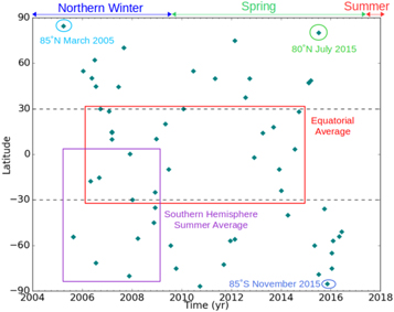
Figure 1. Spatial and temporal distribution of the limb datasets presented in this paper. Teal diamonds represent the available Cassini/CIRS limb data. Spatial averages are indicated with rectangles.
Download figure:
Standard image High-resolution image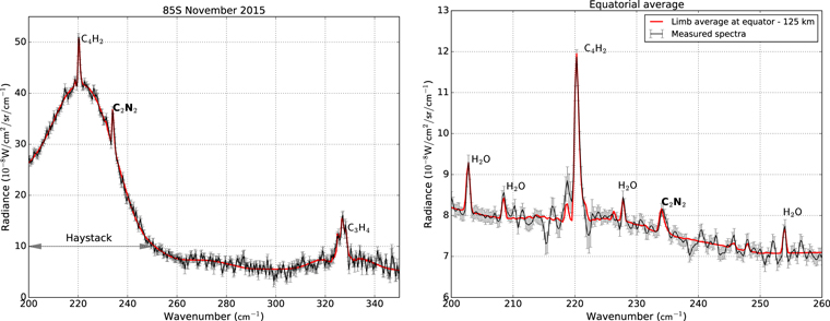
Figure 2. Examples of spectra measured with Cassini/CIRS (black lines) and matching synthetic spectra calculated by NEMESIS (red lines). The spectral resolution is 0.5  data points are spaced by 0.25
  . Left panel: limb spectrum measured at 85°S in 2015 November at 125 km. Note the presence of the haystack feature, which is visible only in limb and nadir far-infrared spectra measured at high latitudes (poleward from 60°) in fall and winter.
  bands are not visible at high latitudes. Right panel: average of all the limb spectra measured at 125 km between 30°N and 30°S over the duration of the Cassini mission (later referenced as equatorial average), with a close-up on the 200–260
  region where the
  ,
,  , and
, and  bands are visible.
Download figure:
Standard image High-resolution imageTable A1. Cassini CIRS Nadir Datasets Analysed in this Study
| Dataset | Date | N | Latitude (°N) |
|---|---|---|---|
| CIRS_000TI_FIRNADCMP017_PRIME† | 2004 Jul 3 | 13 | −35.5 |
| CIRS_003TI_FIRNADCMP002_PRIME† | 2005 Feb 15 | 180 | −18.7 |
| CIRS_005TI_FIRNADCMP002_PRIME† | 2005 Mar 31 | 241 | −41.1 |
| CIRS_00BTI_FIRNADCMP001_PRIME | 2004 Dec 12 | 224 | 16.4 |
| CIRS_013TI_FIRNADCMP004_PRIME† | 2005 Aug 22 | 248 | −53.7 |
| CIRS_019TI_FIRNADCMP002_PRIME† | 2005 Dec 26 | 124 | −0.0 |
| CIRS_021TI_FIRNADCMP002_PRIME† | 2006 Feb 27 | 213 | −30.2 |
| CIRS_022TI_FIRNADCMP003_PRIME†* | 2006 Mar 18 | 401 | −0.4 |
| CIRS_023TI_FIRNADCMP002_PRIME† | 2006 May 1 | 215 | −35.0 |
| CIRS_024TI_FIRNADCMP003_PRIME†* | 2006 May 19 | 350 | −15.5 |
| CIRS_029TI_FIRNADCMP003_PRIME* | 2006 Sep 23 | 312 | 9.5 |
| CIRS_030TI_FIRNADCMP002_PRIME† | 2006 Oct 10 | 340 | −59.1 |
| CIRS_035TI_FIRNADCMP023_PRIME† | 2006 Dec 12 | 164 | −73.3 |
| CIRS_036TI_FIRNADCMP002_PRIME† | 2006 Dec 28 | 136 | −89.1 |
| CIRS_037TI_FIRNADCMP002_PRIME† | 2007 Jan 13 | 107 | −70.3 |
| CIRS_038TI_FIRNADCMP002_PRIME† | 2007 Jan 29 | 254 | −39.7 |
| CIRS_040TI_FIRNADCMP001_PRIME† | 2007 Mar 9 | 159 | −49.2 |
| CIRS_041TI_FIRNADCMP001_PRIME† | 2007 Mar 25 | 2 | −76.8 |
| CIRS_042TI_FIRNADCMP001_PRIME† | 2007 Apr 10 | 103 | −60.8 |
| CIRS_043TI_FIRNADCMP001_PRIME† | 2007 Apr 26 | 263 | −51.4 |
| CIRS_044TI_FIRNADCMP002_PRIME*† | 2007 May 13 | 104 | −0.5 |
| CIRS_045TI_FIRNADCMP001_PRIME† | 2007 May 28 | 231 | −22.3 |
| CIRS_046TI_FIRNADCMP001_PRIME* | 2007 Jun 13 | 60 | 17.6 |
| CIRS_046TI_FIRNADCMP002_PRIME† | 2007 Jun 14 | 102 | −20.8 |
| CIRS_047TI_FIRNADCMP001_PRIME* | 2007 Jun 29 | 204 | 9.8 |
| CIRS_048TI_FIRNADCMP001_PRIME† | 2007 Jul 18 | 96 | −34.8 |
| CIRS_050TI_FIRNADCMP001_PRIME†* | 2007 Oct 1 | 144 | −10.1 |
| CIRS_053TI_FIRNADCMP001_PRIME† | 2007 Dec 4 | 223 | −40.2 |
| CIRS_055TI_FIRNADCMP001_PRIME* | 2008 Jan 5 | 190 | 18.7 |
| CIRS_059TI_FIRNADCMP001_PRIME† | 2008 Feb 22 | 172 | −24.9 |
| CIRS_059TI_FIRNADCMP002_PRIME* | 2008 Feb 23 | 98 | 17.1 |
| CIRS_067TI_FIRNADCMP001_PRIME† | 2008 May 11 | 48 | −59.5 |
| CIRS_069TI_FIRNADCMP001_PRIME† | 2008 May 27 | 112 | −44.6 |
| CIRS_069TI_FIRNADCMP002_PRIME* | 2008 May 28 | 112 | 9.5 |
| CIRS_095TI_FIRNADCMP001_PRIME†* | 2008 Dec 5 | 213 | −14.0 |
| CIRS_097TI_FIRNADCMP001_PRIME†* | 2008 Dec 20 | 231 | −10.9 |
| CIRS_106TI_FIRNADCMP001_PRIME† | 2009 Mar 26 | 165 | −60.3 |
| CIRS_110TI_FIRNADCMP001_PRIME† | 2009 May 6 | 282 | −68.1 |
| CIRS_111TI_FIRNADCMP002_PRIME† | 2009 May 22 | 168 | −27.1 |
| CIRS_112TI_FIRNADCMP002_PRIME† | 2009 Jun 7 | 274 | −58.9 |
| CIRS_114TI_FIRNADCMP001_PRIME† | 2009 Jul 9 | 164 | −71.4 |
| CIRS_119TI_FIRNADCMP001_PRIME† | 2009 Oct 11 | 5 | −25.9 |
| CIRS_119TI_FIRNADCMP002_PRIME* | 2009 Oct 12 | 166 | 0.4 |
| CIRS_123TI_FIRNADCMP002_PRIME† | 2009 Dec 28 | 186 | −46.1 |
| CIRS_124TI_FIRNADCMP002_PRIME* | 2010 Jan 13 | 272 | −1.2 |
| CIRS_131TI_FIRNADCMP002_PRIME* | 2010 May 20 | 229 | −19.8 |
| CIRS_133TI_FIRNADCMP001_PRIME* | 2010 Jun 20 | 187 | −49.7 |
| CIRS_134TI_FIRNADCMP001_PRIME* | 2010 Jul 6 | 251 | −10.0 |
| CIRS_138TI_FIRNADCMP001_PRIME* | 2010 Sep 24 | 190 | −30.1 |
| CIRS_148TI_FIRNADCMP001_PRIME* | 2011 May 8 | 200 | −10.0 |
| CIRS_153TI_FIRNADCMP001_PRIME* | 2011 Sep 11 | 227 | 9.9 |
| CIRS_160TI_FIRNADCMP002_PRIME* | 2012 Jan 30 | 280 | −0.2 |
| CIRS_161TI_FIRNADCMP001_PRIME* | 2012 Feb 18 | 121 | 9.9 |
| CIRS_161TI_FIRNADCMP002_PRIME* | 2012 Feb 19 | 89 | −15.0 |
| CIRS_166TI_FIRNADCMP001_PRIME* | 2012 May 22 | 318 | −19.9 |
| CIRS_169TI_FIRNADCMP001_PRIME* | 2012 Jul 24 | 258 | −9.7 |
| CIRS_175TI_FIRNADCMP001_PRIME* | 2012 Nov 28 | 150 | 15.0 |
| CIRS_185TI_FIRNADCMP001_PRIME* | 2013 Apr 5 | 244 | 15.0 |
| CIRS_190TI_FIRNADCMP001_PRIME* | 2013 May 23 | 224 | −0.2 |
| CIRS_195TI_FIRNADCMP001_PRIME* | 2013 Jul 25 | 186 | 19.6 |
| CIRS_201TI_FIRNADCMP001_PRIME* | 2014 Feb 2 | 329 | 19.9 |
| CIRS_203TI_FIRNADCMP002_PRIME* | 2014 Apr 7 | 239 | 0.5 |
| CIRS_207TI_FIRNADCMP002_PRIME | 2014 Aug 21 | 163 | 79.7 |
| CIRS_248TI_FIRNADCMP001_PRIME | 2016 Nov 13 | 185 | −88.9 |
Note. N is the number of spectra measured during the acquisition. Asterisks denote the datasets used in the equatorial average. † denote the datasets used in the southern summer hemisphere average.
Table A2. Cassini CIRS Limb Datasets Analysed in this Study
| Dataset | Date | N | Latitude (°N) |
|---|---|---|---|
| CIRS_005TI_FIRLMBINT002_PRIME | 2005 Mar 31 | 26 | 84.6 |
| CIRS_013TI_FIRLMBINT002_PRIME† | 2005 Aug 22 | 58 | −54.5 |
| CIRS_013TI_FIRLMBINT003_PRIME† | 2005 Aug 22 | 58 | −54.5 |
| CIRS_028TI_FIRLMBINT002_PRIME*† | 2006 Sep 7 | 54 | −15.3 |
| CIRS_029TI_FIRLMBINT003_PRIME* | 2006 Sep 23 | 70 | 30.0 |
| CIRS_038TI_FIRLMBINT001_PRIME* | 2007 Jan 29 | 26 | 28.7 |
| CIRS_040TI_FIRLMBINT001_PRIME* | 2007 Mar 9 | 35 | 9.6 |
| CIRS_040TI_FIRLMBINT002_PRIME* | 2007 Mar 10 | 29 | 14.8 |
| CIRS_052TI_FIRLMBINT001_PRIME† | 2007 Nov 18 | 24 | −79.9 |
| CIRS_053TI_FIRLMBINT001_PRIME*† | 2007 Dec 4 | 79 | 0.2 |
| CIRS_055TI_FIRLMBINT001_PRIME*† | 2008 Jan 5 | 54 | −29.9 |
| CIRS_062TI_FIRLMBINT003_PRIME† | 2008 Mar 25 | 49 | −55.3 |
| CIRS_093TI_FIRLMBINT002_PRIME† | 2008 Nov 19 | 74 | −44.9 |
| CIRS_095TI_FIRLMBINT001_PRIME† | 2008 Dec 5 | 54 | −35.1 |
| CIRS_095TI_FIRLMBINT002_PRIME*† | 2008 Dec 5 | 76 | −25.0 |
| CIRS_097TI_FIRLMBINT001_PRIME* | 2008 Dec 21 | 55 | 10.1 |
| CIRS_110TI_FIRLMBINT001_PRIME* | 2009 May 5 | 51 | 20.1 |
| CIRS_113TI_FIRLMBINT001_PRIME*† | 2009 Jun 22 | 59 | −10.0 |
| CIRS_115TI_FIRLMBINT002_PRIME† | 2009 Jul 24 | 51 | −60.0 |
| CIRS_119TI_FIRLMBINT002_PRIME† | 2009 Oct 12 | 60 | −75.0 |
| CIRS_125TI_FIRLMBINT001_PRIME* | 2010 Jan 29 | 68 | 29.9 |
| CIRS_175TI_FIRLMBINT001_PRIME* | 2012 Nov 29 | 70 | −2.0 |
| CIRS_185TI_FIRLMBINT001_PRIME* | 2013 Apr 5 | 70 | 14.0 |
| CIRS_200TI_FIRLMBINT002_PRIME* | 2014 Jan 1 | 49 | −24.0 |
| CIRS_206TI_FIRLMBINT005_PRIME* | 2014 Jul 20 | 65 | 3.5 |
| CIRS_208TI_FIRLMBINT002_PRIME* | 2014 Sep 22 | 70 | 28.1 |
| CIRS_218TI_FIRLMBINT001_PRIME | 2015 Jul 7 | 51 | 80.1 |
| CIRS_225TI_FIRLMBINT002_PRIME | 2015 Nov 13 | 53 | −84.6 |
Note. N is the number of spectra measured during the acquisition. Asterisks denote the datasets used in the equatorial average. † denote the datasets used in the southern hemisphere summer average.
Download table as: ASCIITypeset image
2.2. Retrieval Method
Figure 2 shows examples of limb spectra in the  range. We measure the abundance of
  using its ν5 band at
  . Other spectral features are visible such as the ν9 band of
  at
at  , ν10 band of
  at
at  , and several absorption bands of
  , for instance at
  ,
,  ,
,  , and
, and  . We retrieve the abundances of these gases using the constrained non-linear inversion code Non-linear Optimal Estimator for MultivariatE Spectral analySIS (NEMESIS; Irwin et al. 2008). NEMESIS uses an iterative algorithm where a synthetic spectrum is calculated from a reference atmosphere and a priori values for the retrieved parameters. For each iteration, these values are updated to minimize the difference between the measured and the synthetic spectra, until convergence is reached and the improvement in misfit is less than 0.1%.
We adopt the same reference atmosphere as Sylvestre et al. (2018) which takes into account the abundances of the main constituents of Titan's atmosphere, as measured by Cassini/CIRS, Cassini/Visible and Infrared Mapping Spectrometer (VIMS), Atacama Large Millimeter/submillimeter Array (ALMA), and Huygens/Gas Chromatograph Mass Spectrometer (GCMS). The composition of this reference atmosphere and the relevant references are fully detailed in Sylvestre et al. (2018).
Aerosol properties and vertical distributions are derived from previous Cassini/CIRS measurements of de Kok et al. (2007, 2010) and Vinatier et al. (2012), with the four types of hazes described in de Kok et al. (2007): hazes 0 ( to
to  ), A (centered at
  ), B (centered at
  ), and C (centered at
  ).
).
Spectroscopic parameters are the same as in Sylvestre et al. (2018), except for the Collision Induced Absorption coefficients (CIA). We adopted the model presented in Bézard & Vinatier (2020), where the coefficients for the  CIA from Borysow & Tang (1993) and the
  CIA from Borysow & Frommhold (1986a) are multiplied by the following factors:


where T, Tsat, and σ are respectively local temperature,  saturation temperature, and wavenumber. Coefficients for
  and
and  CIA remain the same as in Borysow & Frommhold (1986b, 1987).
For each of the cases presented in Figure 1, limb and nadir spectra were fitted individually as follows.
Southern summer hemisphere average and 80°N in 2015 July. For each limb spectrum, we retrieved scale factors toward the nominal profiles of  ,
,  ,
,  ,
,  , and the four types of hazes previously defined. The effect of the large field of view of the CIRS FP1 limb data was taken into account by dividing their field of view into M parts, generating synthetic spectra for each of these parts, and using a weighted average of these spectra, as described in Teanby & Irwin (2007). We chose M = 11 so that the errors in the modeled radiance stay smaller than the measurement noise. We set the temperature profiles for the considered latitudes and dates using previous Cassini/CIRS measurements of Sylvestre et al. (2020) and Teanby et al. (2019). For each gas, we used the abundances retrieved from the two limb spectra (at 125 km and 225 km) to build a priori profiles for the nadir retrievals. We then retrieved
  ,
,  ,
,  , and
, and  scale factors from the nadir spectra using these a priori profiles. We also retrieved simultaneously scale factors for hazes 0, B, and C and a temperature profile (as the tropospheric temperature contributes to the continuum emission of the nadir spectra).
85°N in 2005 March and 85°S in 2015 November. The previous method had to be adapted to these datasets in order to fit the haystack feature (see Figure 2) in both limb and nadir spectra. We retrieved the cross-sections of haze B for each spectrum while keeping the vertical distribution measured in de Kok et al. (2007). We also retrieve simultaneously scale factors for  ,
,  ,
,  ,
,  and haze 0 profiles, and a temperature profile (only for the nadir spectra).
Equatorial average. We follow a method similar as in the first case, except that this time, it was necessary to fit new cross-sections for haze 0 in each limb spectrum while scale factors were retrieved for hazes B and C. This difference could be due to the fact that the equatorial average was made by averaging CIRS spectra over 8 yr, unlike the other datasets where spectra were measured at a single date or over a half a season (2005–2009 for the southern hemisphere summer average).
Errors due to measurement noise, forward modeling, and smoothing of the profiles by NEMESIS are on the order of 10% on average. For the equatorial average, as we used an average temperature profile as a priori, we assess the effects of temperature variations on the considered latitude and time range by retrieving these datasets using the coldest and warmest temperature profiles measured at the equator over the Cassini mission. We found that the errors due to temperature variations are also about 10%.
For each dataset, the level of detection of a gas can be assessed by calculating the change in the misfit Δχ2, defined as

with

where Imes and Ifit are respectively the measured and fitted radiance, at a given wavenumber wi and for a value x of the abundance of the considered gas. σi is the measurement error at wi. The factor 2 at the denominator is to calculate the χ2 for the correct number of independent points, as spectra have a sampling interval of 0.25  while their spectral resolution is 0.5
  .
.  is the value of χ2 with x = 0. In the datasets presented here,
  and
and  were always detected at more than 3σ (Δχ2 ≤ −9). When
  and
and  were not detected at 3σ, we looked for their 3σ upper limits, i.e., the value x for which Δχ2 = 9. This was especially relevant at the poles, where water could not be detected at more than 1 − σ, and for
  which could not be detected at the equator at 225 km.
Figure 3 shows the normalized contribution functions for  (at
(at  ),
),  (at
(at  ),
),  (at
(at  ), and
  (at
(at  ). Taking into account their field of view, the combination of limb and nadir data are sensitive in the 75-265 km altitude range for
  ,
,  and
and  , and in the 90-265 km range for
  .
.  and
and  contribution functions are similar for the equatorial average and 85°S in 2015. However, the cold polar temperatures of southern fall increase the altitude at which
  condenses, shift the contribution function of the nadir spectra upwards (from 85 km to 95 km), and make the contribution function of the limb spectrum at 125 km narrower.
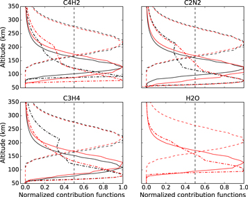
Figure 3. Normalized contribution functions for the equatorial average (in red) and 85°S in 2015 November (in black). Solid and dashed lines represent respectively the contribution functions for the limb data at 125 km and 225 km. Dotted–dashed lines stand for nadir data. The combination of the limb and nadir FP1 data allows for the measurement of  ,
,  ,
,  in the 75–265 km range, and
  between 90 km and 245 km. Note that the contribution functions of the equatorial average and for 85°S in 2015 November are often very similar (and hence superimposed), except for the
  nadir and 125 km limb spectra, as the cold polar temperatures shift the
  condensation level upward.
Download figure:
Standard image High-resolution image3. Results and Discussions
3.1.
 and
and


In Figure 4 we present the results of our limb and nadir measurements for  ,
,  ,
,  , and
, and  .
.
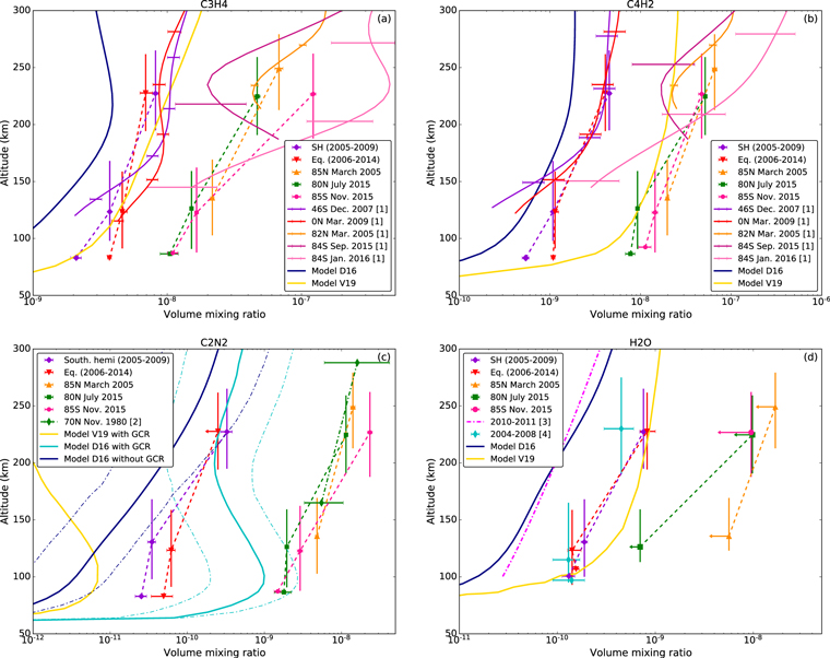
Figure 4. Vertical profiles of  ,
,  ,
,  , and
, and  . Markers indicate the volume mixing ratios measured from limb and nadir measurements. Vertical lines represent the field of view of the limb data. Dashed lines help to visualize the vertical variations of these four species. V19 and D16 stand respectively for the nominal photochemical model predictions of Vuitton et al. (2019), Dobrijevic et al. (2016), and Loison et al. (2019). Panels (a) and (b): [1] indicates the Cassini/CIRS limb measurements of Mathé et al. (2020). Panels (c) and (d): [2], [3], and [4] are respectively the measurements of Coustenis et al. (1991) with Voyager 1/IRIS, Moreno et al. (2012) with Herschel/PACS and HIFI, and Cottini et al. (2012) with Cassini/CIRS. In panel (c), the uncertainties around the profiles of model D16 are shown for
  as thin dotted–dashed lines.
Download figure:
Standard image High-resolution imageWe show our measurements of  in panel (a) and
  in panel (b). With our equatorial limb and nadir spectral averages over the Cassini mission, we obtained profiles of
  and
and  that are increasing with altitude (from
  at 85 km to
  at 225 km for
  , and from
  at 85 km to
  at 225 km for
  ). Previous Cassini/CIRS studies showed that below 300 km, at the equator, trace gas abundances vary weakly throughout the Cassini mission (e.g., Mathé et al. 2020; Teanby et al. 2019). The volume mixing ratios retrieved from our equatorial spectral average should thus be comparable to previous individual measurements at specific times during the Cassini mission. For instance Figure 4 shows that our profiles of
  are in very good agreement with the results of Mathé et al. (2020) with Cassini/CIRS FP3 measurements at 0°N in March 2009, while we measured slightly smaller abundances than them for
  . Lombardo et al. (2019a) averaged Cassini/CIRS FP3 limb spectra acquired between 20°S and 20°N from 2004 to 2009 and found a nearly constant with altitude volume mixing ratio of 1 × 10⁻⁸ between 110 km and 400 km, which is also slightly larger than our results. These differences can be explained by the characteristics of the compared datasets, especially the different vertical coverages and resolutions (10 to 50 km for the limb data of Lombardo et al. 2019a; Mathé et al. 2020), the use of detectors operating in different wavelengths, and thus the use of different spectroscopic data. Our results are also consistent with the nadir CIRS FP3 measurements from Coustenis et al. (2019) who measured volume mixing ratios of 4.9 ± 1 × 10⁻⁹ for
  and 1.1 ± 0.3 × 10⁻⁹ for
  at 10 mbar (100 km) at the equator in 2017, and nadir measurements of Teanby et al. (2019) who found average abundances of 9 × 10⁻⁹ for
  and 2 × 10⁻⁹ at 1 mbar (180 km) at the equator throughout the Cassini mission.
We observe a similar situation when comparing the  and
and  profiles measured from our limb and nadir spectral averages over the southern hemisphere in summer (2005–2009) with Mathé et al. (2020) at 46°S in December 2007, the measurements of Coustenis et al. (2019) and Teanby et al. (2019), and the average profile of
  in the southern hemisphere measured by Lombardo et al. (2019a) in 2004–2009 (20°S-60°S). Besides, Coustenis et al. (2019), Mathé et al. (2020), and Teanby et al. (2019) showed that trace gas abundances remain fairly constant below 300 km throughout southern summer. Consequently our equatorial and summer southern hemisphere averages seem to capture fairly well the composition of Titan's atmosphere in the lower atmosphere, despite the large latitude and time ranges used. Besides, using nadir FP1 data allows us to probe lower altitudes (down to 85 km) than the studies cited above, and thus to complete them with information about the lower part of the stratosphere, as shown in Sylvestre et al. (2018) and Lombardo et al. (2019b). For instance, Figure 4 shows that in summer, abundances of
  and
and  in the southern hemisphere are smaller than at the equator at 85 km (by a factor of 2 for
  ), while they are similar for both latitudes above 125 km and up to 360 km for
  and 440 km for
  . When compared to the predictions of the photochemical models, the
  profile measured at the equator is in good agreement with the predictions of Vuitton et al. (2019; model V19 on Figure 4). The model of Dobrijevic et al. (2016) and Loison et al. (2019; model D16 on Figure 4) underestimates the abundance of this gas by up to a factor of 10 at 85 km. The abundances predicted by Dobrijevic et al. (2016) and Loison et al. (2019) for
  are also smaller than the abundances we measured at the equator (by up to a factor of 10) at 85 km. The nominal model of Vuitton et al. (2019) overestimates by a factor of 10
  abundances, but their model without H heterogeneous loss (loss of hydrogen atoms when they interact with the surface of aerosols) is in very good agreement with our CIRS measurements. This is consistent with what Mathé et al. (2020) noted with their own CIRS observations at higher altitudes.
At high latitudes, we measure an enrichment in  and
and  compared to the equator (by a factor of 17 for
  and 10 for
  at 85°S in 2015 November at 225 km). This is in good agreement with the results from previous studies (e.g., Coustenis et al. 2019; Mathé et al. 2020; Teanby et al. 2019), especially if we take into account the strong dynamical activity and rapid evolution of the poles, for instance when the south pole goes from fall to winter solstice, as illustrated by the differences between the profiles measured at 84°S in 2015 September and 2016 January by Mathé et al. (2020; see Figure 4), and as described by Teanby et al. (2017). This is due to the atmospheric circulation that evolves from two equator-to-poles cells at the equinox, to a single pole-to-pole cell with a strong subsidence above the fall/winter pole that advects photochemical products from their production area in the upper atmosphere to the lower atmosphere, as shown in Titan's General Circulation Models (GCM; Vatant d'Ollone et al., in preparation; Newman et al. 2011; Lebonnois et al. 2012; Lora et al. 2015; Vatant d'Ollone et al. 2017). At high northern latitudes,
  and
and  abundances have decreased slightly from 2005 March to 2015 July, i.e., from winter to late spring. This confirms previous observations of Sylvestre et al. (2018; at 85 km) and Mathé et al. (2020; in the 175–280 km altitude range) where the enrichment in photochemical species at the north pole persists up to 2015 January in the lower stratosphere, whereas a depletion is observed in the upper stratosphere from 2011 December (Vinatier et al. 2015; Mathé et al. 2020). These observations are consistent with the persistence of a small circulation cell above the high northern latitudes during the transition from the two equator-to-poles cells to a single pole-to-pole during most of the northern spring as predicted by the Laboratoire de Météorologie Dynamique Zoom (LMDZ) GCM (Vatant d'Ollone et al. 2017; Lebonnois et al. 2012; see also Figure 12 of Sylvestre et al. 2018). In 2015 July, this residual circulation cell has disappeared, thus allowing the depletion in trace gases of the lower stratosphere by upwelling.
3.2.

Panel (c) of Figure 4 shows the  profiles we measured at different latitudes and seasons. At the equator, we measured an average profile over the Cassini mission where
  increases from 5.0 ± 1.5 × 10⁻¹¹ at 85 km to 6.2 ± 0.8 × 10⁻¹¹ at 125 km, and a 3σ upper limit of 2.5 × 10⁻¹⁰ at 225 km. In the southern hemisphere in summer (2005–2009) we were able to measure an abundance of 6.8 ± 0.6 × 10⁻¹⁰ for
  at 225 km. The
  abundances retrieved from the southern summer dataset below 225 km are smaller than the abundances at the equator, similar to what was measured for
  and
and  . The LMDZ GCM predicts that during northern winter the upwelling due to the ascending branch of the pole-to-pole cell is the strongest above southern mid-latitudes. Air depleted in photochemical products (due to their condensation) is thus advected upward in the southern hemisphere, which explains why it has lower
  ,
,  , and
, and  than at the equator.
At high latitudes, our measurements are consistent with the profile at 70°N by Coustenis et al. (1991).  profiles exhibit a strong enrichment compared to our equatorial or southern hemisphere summer averages. This trend is similar to the measurements of
  at 15 mbar (85 km) by Sylvestre et al. (2018), and to what has been measured for
  and
and  . The seasonal evolution of
  at high northern latitudes is also very similar to the evolution of
  and
and  , with a slight decrease from northern winter (2005) to late spring (2015). The enrichment in
  at the poles is much larger than the enrichment in
  and
and  . For instance, in our results, 85°S in 2015, the
  volume mixing ratio at 225 km was at least 100 times larger than at the equator, whereas
  and
and  abundances were respectively 17 and 10 times larger than at the equator. This is consistent with the results of Teanby et al. (2010) where nitriles were more enriched than hydrocarbons with similar photochemical lifetimes, which could indicate the presence of an additional loss process for nitriles.
In Figure 4, the CIRS profiles of  are compared with the profiles predicted by the photochemical models of Vuitton et al. (2019; model V19 in Figure 4) and of Dobrijevic et al. (2016) and Loison et al. (2015; model D16 in Figure 4). The abundances we measured at the equator and in the southern hemisphere in summer are the same order of magnitude as the predictions of Dobrijevic et al. (2016) and 1–2 orders of magnitude larger than the results of Vuitton et al. (2019). This may be explained by the different chemical reaction schemes of these two models, and more particularly in the main production reactions for
  , which for Vuitton et al. (2019) is

and for Dobrijevic et al. (2016) is

which is not taken into account into the model of Vuitton et al. (2019). However, significant uncertainties remain about the kinetics of reaction 6 (V. Vuitton, personal communication). In both models, the main loss reaction in the lower stratosphere is

unlike the photochemical model of Krasnopolsky (2014), where  is mainly lost by photodissociation and where the
  abundance is overestimated by a factor of 60.
GCRs ionize  in the lower stratosphere with a magnitude comparable to solar UV in the upper atmosphere (Gronoff et al. 2009), hence creating a second production region for
  at lower altitude in photochemical models. In Vuitton et al. (2019) and Dobrijevic et al. (2016), instead of increasing with altitude like
  abundance, the
  profile exhibits a local maximum between 100 km and 200 km (see Figure 4). Below 100 km,
  abundance decreases with decreasing altitude as this gas reacts with other species and condenses. When we compare the profiles of
  from Dobrijevic et al. (2016) with and without GCRs, our measurements at the equator and in the southern hemisphere in summer are in good agreement with the profile with GCRs at 225 km, but not in agreement with either profiles below 125 km, where photochemical models predict a local maximum of
  due to the GCR. This seems to indicate a smaller influence of the GCR on the
  profile than predicted by the models. However, their effect cannot be completely ruled out as we do not observe the steep decrease with pressure predicted without GCRs.
Many other nitrogen-bearing species are predicted to be affected by the GCR bombardment. For instance, in Dobrijevic et al. (2016), HNC is predicted to be up to 100 times more abundant below 600 km when effects of GCR bombardment are included. However, recent ALMA measurements of the vertical profile of HNC are in better agreement with the predictions of Dobrijevic et al. (2016) without the effects of GCRs (Lellouch et al. 2019). GCRs may also have a strong effect on the  ratios in
  and
and  , as they could be up to twice as high as in HCN or
  (Dobrijevic & Loison 2018). Iino et al. (2020) ALMA measurements of
  in
in  were not inconsistent with these predictions, but not precise enough to be conclusive. The production of amines (e.g.,
  ,
,  ,
,  ), imines (e.g.,
  ), and aromatics could also be increased by the GCR (by up to 3 orders of magnitude for amines and imines; Loison et al. 2015, 2019), but observational data are insufficient for these species.
3.3.

Panel (d) of Figure 4 presents our measurements for the  abundances. At the equator, the abundance of water increases with altitude from 1.6 ± 0.1 × 10⁻¹⁰ at 100 km to
  at 225 km. In the lower atmosphere, our results are consistent with the Cassini/CIRS measurements of Cottini et al. (2012; see Figure 4) and of Bauduin et al. (2018), and about one order of magnitude larger than the Herschel measurements of Moreno et al. (2012). Bauduin et al. (2018) explained the inconsistency between the CIRS and Herschel results by potential meridional and seasonal variations in
  abundance. At 225 km, we measured a
  abundance twice as large as Cottini et al. (2012). In the southern hemisphere in summer,
  abundance is within error bars from the equatorial measurements at all probed altitudes unlike
  ,
,  and
and  for which volume mixing ratios are significantly smaller in the southern hemisphere than at the equator below 125 km. This difference of behavior is expected as
  is predicted to have a much longer lifetime than
  ,
,  , and
, and  . At the poles, we could only measure 3σ upper limits of
  which allow us to say that fall/winter poles cannot be enriched in water by more than a factor of 10 compared to the equator at 225 km. These results are not inconsistent with the meridional and seasonal variations in water distribution suggested by Bauduin et al. (2018) to explain the differences between the Cassini/CIRS and the Herschel results.
Our  profiles are also compared to the photochemical models of Dobrijevic et al. (2016), Loison et al. (2019; model D16 in Figure 4), and Vuitton et al. (2019; model V19 in Figure 4). The profile from Vuitton et al. (2019) is in good agreement with our measurements at the equator and in the southern hemisphere in summer whereas the predictions of Dobrijevic et al. (2016) and Loison et al. (2019) are one order of magnitude smaller than our results. As Dobrijevic et al. (2016) used the results of Moreno et al. (2012) to constrain the eddy diffusion coefficient in their model, the good agreement between these two studies is expected. More measurements of
  abundance are required to constrain further its variations and understand the processes that shape its vertical and meridional distribution.
4. Conclusion
In this paper, we present the first study of the  vertical distribution for different latitudes and seasons in Titan's stratosphere, using Cassini/CIRS measurements. At the equator we measured a
  abundance increasing with altitude, from 5.0 ± 1.5 × 10⁻¹¹ at 85 km to 6.2 ± 0.8 × 10⁻¹¹ at 125 km and a 3σ upper limit of 2.5 × 10⁻¹⁰ at 225 km. Poles are enriched in
  , by up to a factor of 100 compared to the equator. Comparing these vertical profiles with the predictions of recent photochemical models helps to constrain the chemistry of this gas, especially on the role of the GCRs that seem less important than predicted in the models. These data also allowed us to measure profiles of
  and
and  in the lower part of the stratosphere (down to 85 km), which is usually not probed by mid-infrared Cassini/CIRS observations. We could thus extend the description of the meridional and seasonal variations of these species to this part of Titan's atmosphere. This study also provides insights on the variations of the
  abundance in Titan's lower atmosphere, including upper limits on its potential enrichment by the atmospheric circulation at the poles (up to a factor of 10).
This research was funded by the UK Sciences and Technology Facilities Research council (grant number ST/R000980/1) and the Cassini project. This research made use of Astropy, a community-developed core Python package for Astronomy (Astropy Collaboration et al. 2013), and matplotlib, a Python library for publication quality graphics (Hunter 2007). We thank Jan Vatant d'Ollone for insightful discussions about the predictions of the LMDZ GCM, Véronique Vuitton for useful comments about Titan's photochemistry, and the anonymous reviewer for their suggestions.