Post-Processing and Evaluation of Precipitation Ensemble Forecast under Multiple Schemes in Beijiang River Basin


1
Center for Water Resources and Environment, Sun Yat-sen University, Guangzhou 510275, China
2
Guangdong Research Institute of Water Resources and Hydropower, Guangdong Engineering Laboratory of Estuary Hydropower, Guangzhou 510635, China
*
Author to whom correspondence should be addressed.
Water 2020, 12(9), 2631; https://doi.org/10.3390/w12092631
Submission received: 8 August 2020
/
Revised: 13 September 2020
/
Accepted: 17 September 2020
/
Published: 21 September 2020
(This article belongs to the Section Hydrology)
Abstract
:Precipitation is one of the most important factors affecting the accuracy and uncertainty of hydrological forecasting. Considerable progress has been made in numerical weather prediction after decades of development, but the forecast products still cannot be used directly for hydrological forecasting. This study used ensemble pro-processor (EPP) to post-process the Global Ensemble Forecast System (GEFS) and Climate Forecast System version 2 (CFSv2) with four designed schemes, and then integrated them to investigate the forecast accuracy in longer time scales based on the best scheme. Many indices such as correlation coefficient, Nash efficiency coefficient, rank histogram, and continuous ranked probability skill score were used to evaluate the results in different aspects. The results show that EPP can improve the accuracy of raw forecast significantly, and the scheme considering cumulative forecast precipitation is better than that only considers single-day forecast. Moreover, the scheme that considers some observed precipitation would help to improve the accuracy and reduce the uncertainty. In terms of medium- and long-term forecasts, the integrated forecast based on GEFS and CFSv2 after post-processed would be better than CFSv2 significantly. The results of this study would be a very important demonstration to remove the deviation of ensemble forecast and improve the accuracy of hydrological forecasting in different time scales.
1. Introduction
Flood is a hazard with potentially serious consequences of loss of life and economic costs which occur more frequently with the impact of climate change and human activities [1,2]. Hydrological forecasting has been proven to be an effective non-engineering measure to resist flood disasters and reduce losses; its accuracy depends on the input precipitation data [3]. Therefore, improving the accuracy of precipitation forecast is an effective way to improve the accuracy of hydrological forecast. Many studies have shown that numerical weather prediction (NMP) and climate models can improve the skills of precipitation forecast significantly [4,5,6,7,8].
With the rapid development of computer technology and meteorological science, the meteorological ensemble prediction is superior to the traditional one in terms of forecast accuracy and period, and it has been widely accepted by many national meteorological departments [9]. Moreover, The Canadian Meteorological Centre (CMC), the European Centre for Medium-Range Weather Forecasts (ECMWF), the National Centers for Environmental Prediction (NCEP), and the China Meteorological Administration (CMA) have all realized the operation of numerical ensemble prediction [10]. At present, the Global Ensemble Forecast System (GEFS) [11], Climate Forecast System (CFS) [12], and THORPEX (The Observing System Research and Predictability Experiment) Interactive Grand Global Ensemble (TIGGE) [13] are the most representative products in the world. In addition, GEFS and CFS both have more than 30 years of meteorological ensemble database, which are operated by the NCEP and have developed to the second version of reanalysis and forecast system. Aiming to accelerate the improvements in the accuracy of one-day to two-week high-impact weather forecasts, the World Meteorological Organization launched a 10-year plan (2005–2015) of THORPEX and established the TIGGE database, which consists of ensemble forecast data from 10 global NWP centers, starting from October 2006 [13]. In addition, TIGGE can satisfy users’ various information needs such as the development of observation systems, forecasting systems, and data assimilation. Scholars have done a lot of research based on meteorological ensemble forecast. Liu et al. [14] evaluated the GFS forecast precipitation after ensemble pre-processing based on the measured data of meteorological stations in the Huaihe River, and found that the accuracy of precipitation in the early stage is higher than that in the later stage, while the accuracy of accumulated precipitation is higher than that of single day.
Although the meteorological ensemble forecast has been greatly improved in terms of accuracy and forecast period, it cannot be used to drive the hydrological model directly and needs to be processed for spatial downscaling and deviation correction. The core idea of the processing method is to establish a statistical relationship between the meteorological elements derived from the weather model and the corresponding measured hydrological elements for analysis. For example, the earliest Perfect Prognosis, as proposed by Klein et al. [15], directly applied the statistical relationship between different observed meteorological elements to the output by the model. The Model Output Statistics (MOS) proposed by Glahn et al. [16] uses multiple regression to establish the statistical relationship between observations and model outputs. Rank histograms [17], Bayesian processor method [18], quantile mapping method [19], and ensemble pre-processor [20,21] have all greatly promoted the development and application of NWP. This kind of methods have a certain good performance when dealing with most meteorological elements, but not with precipitation, due to precipitation may not happen at some time, which is difficult to simulate the statistical fitting distribution.
Quantile mapping is a relatively simple empirical method that connects the cumulative probability distribution of observed elements with that of forecast ones, and has been widely applied. For example, Verkade et al. [22] used it to correct the deviation of ECMWF precipitation and temperature forecast data, Zhu et al. [23] used it to correct the deviation of precipitation forecast in GEFS, and Hashino et al. [24] and Wood et al. [25] applied it to the runoff forecast deviation correction. They found that this method has a good effect of deviation correction. However, it does not have stability and reliability due to the limitations of the method itself [26,27].
The main idea of Bayesian method is to establish statistical relationship between historical observation and ensemble forecast, and then obtain conditional probability distribution function of observation corresponding to ensemble forecast [28]. For the non-normally distributed variables, Bayesian first performs the normal quantity transform (NQT), and then obtains the possible original field of observation through the inverse function of NQT after calculating the conditional probability of the observation. Krzysztofowicz et al. [29] verified that the result of Bayesian method is better than that of the traditional statistical model.
The Bayesian method has effectively promoted the research on post-processing methods. Schaake et al. [20] proposed the ensemble pre-processor (EPP) to turn the meteorological ensemble forecast by fitting the probability distribution function to generate ensemble members. Finally, the ensemble average of forecast members is taken as the processing result of numerical weather forecast based on measured data. Moreover, considering the spatiotemporal continuity of ensemble members, Clark et al. [30] and Schaake et al. [20] proposed the “Schaake shuffle” to make the ensemble members have continuous time information, thereby reducing forecast errors. This method is widely used in the world. Liu et al. [31] corrected the deviation of the 15-member daily precipitation forecast from NCEP GFS data in China’s Huai River basin by Schaake method and tested them by the observed data of 167 meteorological stations. Tao et al. [32] used this method to compare the accuracy of five ensemble forecast data sources of TIGGE (CMA, ECMWF, JMA, NCEP, and UKMO) before and after correction and found that the EPP improved the accuracy of the five data sources.
The purpose of this study was to post-process the ensemble forecast by EPP, investigate the better schemes to improve the accuracy of precipitation forecast from GEFS and CFSv2 based on observed data in the Beijiang River Basin (BJR) and explore a way to improve the accuracy of long-term forecasts. This paper is organized as follows. The study area and the main methods used in this study are described in Section 2 and Section 3. The main results and a discussion on the variability of dryness/wetness are presented in Section 4. The conclusions are provided in Section 5.
2. Study Area and Data
2.1. Study Area
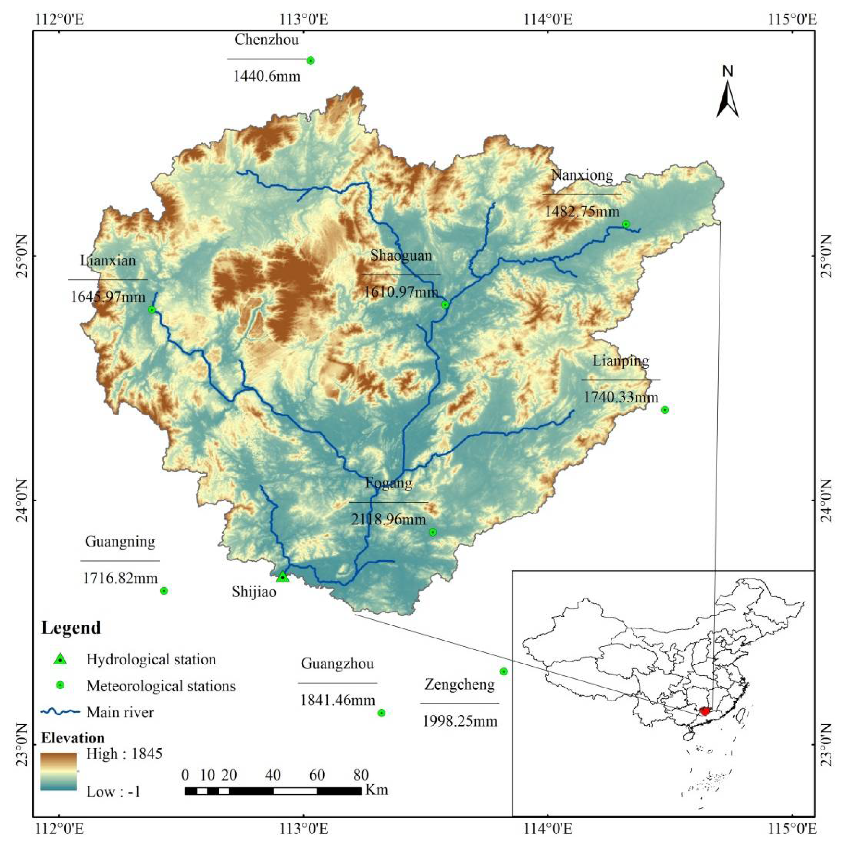
Beijiang River is the secondary tributary of the Pearl River, with an average annual runoff of 42.7 billion m3. The BJR (23°30′–25°42′ N, 112°6′–114°42′ E) is located in the lower reaches of the Pearl River Basin, north of Guangdong Province. The drainage area above Shijiao hydrological station is about 38,670 km2. The terrain of the BJR is mainly mountainous and hilly with the surface elevation of −1 to 1845 m and the terrain slopes of 0–72.79°; the mean slope is 13.37 in this basin. The BJR is a typical subtropical monsoon humid area in southern China, with an average annual rainfall of 1844 mm, of which about 80% of the precipitation is concentrated in the flood season. The historical flood disasters are more serious and directly threaten the Pearl River Delta in the lower reaches of the basin.
2.2. Data
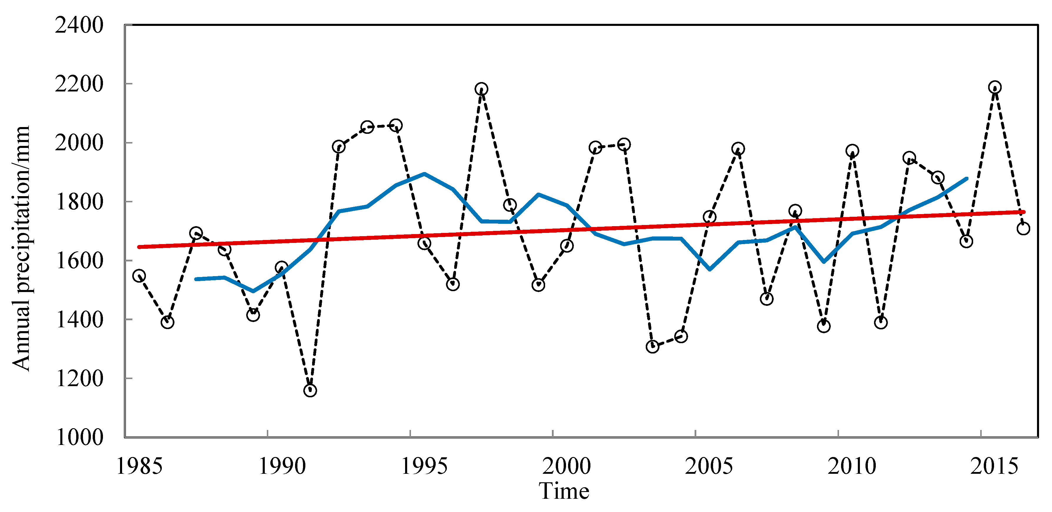
The daily observed precipitation data from meteorological stations (Figure 1 and Table 1) in the BJR were obtained from the China Meteorological Data Network (http://data.cma.cn/). The time span of the dataset is 1 January 1960–31 December 2015. The missing values and outliers in the dataset were verified and disposed using the inverse distance weighted method. The detailed information of the stations is displayed in Table 1, and the annual precipitation over the basin is showed in Figure 2.
The GEFS and CFSv2 used in this study were both provided by NCEP. The GEFS is a weather forecast model using the breeding scheme [33] to generate ensemble perturbations accounting for the uncertainty of initial conditions for medium-range ensemble prediction [11]. The model consists of 11 ensemble members with daily forecast from December 1984 to the present, beginning with 00 UTC (Coordinated Universal Time) every day, and uses an Eulerian horizontal resolution of T254 for the first 8 days of the forecast and T190 for the second 8 days with the data format of Grib2. The dataset contains multiple weather variables such as tropical cyclone, temperature, precipitation, wind etc., of which precipitation is the focus of this paper.
The CFSv2 is a fully coupled atmosphere–ocean–land model developed from four independently designed pieces of technology [30]. It uses the latest scientific methods to collect or assimilate a variety of data sources including ground observations, high-altitude balloon observations, aircraft observations, and satellite observations. The model has updated forecast data of multiple variables (e.g., Madden–Julian oscillation, sea surface temperature, 2-m air temperature, and precipitation) around the world from 1982 to March 2011, with 9-month hindcasts of every 5 days and 4 forecast cycles of that day, i.e., 00, 06, 12, and 18 UTC, and the same hindcasts of daily data from April 2011 to present, at a spatial resolution of 0.938° × 0.938°.
3. Methodology
3.1. Ensemble Pre-Processor
Tremendous progress has been made in the numerical weather and climate models mentioned above over the past decades, but the forecasts generated by those models still contain many deviations and uncertainties. EPP is a useful method that post-processes the ensemble forecasts from these models, reduces the deviations and uncertainties, and prepares precipitation ensemble forecasts for hydrological models. This method transforms the time series of single-value quantitative precipitation forecasts into corresponding ensemble forecasts of precipitation.
(1) Time window
As both the observed and forecasted precipitation would have values of 0, the regression analysis cannot be performed when single-day is selected in this case. The solution is to calculate a proper time window, extract all the data in the time window of given day of each year for statistical regression analysis, to increase the significance of statistical relationships. The time window selection range of this study is 15–30 days before and after given day, which means the total number range of samples in the time window is 31–61. The prerequisite for determining the time window of each given day is to ensure that enough samples can be taken for analysis.
(2) Precipitation threshold
It is considered that precipitation has not occurred if the precipitation value is less than the precipitation threshold. The method of determining the precipitation threshold is to arrange the single-value precipitation series of ensemble forecast in descending order. If the precipitation sequence X = {x1, x2,…, xn}, the precipitation threshold xm can be determined by the following formula.
As long as the percentage p value (e.g., 0.97) is determined, the precipitation threshold can be calculated.
(3) Canonical events
The purpose of canonical events is to extract useful information and eliminate forecast errors to establish a statistical relationship between historical observations and forecasts, so as to correct deviation of future forecast precipitation and reduce uncertainty. The premise of establishing canonical events model is to find events with high correlation from historical observed and forecasted data. According to the theory of chaos in the atmospheric system proposed by Lorenz [34], any forecast of meteorological elements over 5 days is not reliable, but this does not mean that is completely useless [32]. Specifically, GEFS and CFSv2 contain forecast data of multiple lead times; the forecast over the lead time of 5 days is not necessarily reliable, but the accumulated precipitation still contains useful information. For example, the single-day precipitation forecasts from the 6–15-day lead times are not suitable for canonical events since it has a weak correlation with the observed precipitation at the corresponding time. However, the cumulative precipitation forecasts of the 6–15-day lead times can be regarded as a canonical event if it has a good correlation with the observed data. The construction of the joint probability distribution of the measured and predicted meteorological element is based on the canonical events.
(4) Conditional distribution
The construction process of the conditional distribution of canonical events includes designing canonical event, calculating the marginal distribution of measured and forecasted precipitation, converting the marginal distribution into a standard normal distribution, and forming the conditional distribution of observations for a given precipitation forecast.
Assuming that X represents the forecast series, Y represents the observation series, the time window has been calculated to be w, and the time series length of the research data is n years. Then, the canonical events can be displayed as and , and their marginal distribution can be expressed as
If , , then , . and represent the probability of forecasted and observed precipitation respectively. and represent the cumulative probability distribution of forecasted and observed precipitation when it rained, respectively. and represent the cumulative probability distribution of forecasted and observed precipitation. The cumulative probability distribution can be fitted by Gamma, Weibull, or exponential distribution. The Gamma distribution is used in this paper.
It is difficult to find the joint distribution of forecasted and observed precipitation since they are non-normally distributed. The EPP converts the marginal distribution into the standard normal by the NQT to reach the purpose. The conversion process can refer to Ye et al. [35].
The correspondence can be expressed as follows
According to the sampling results of the random variables U and V in the normal distribution space, through the inverse function of the NQT, the conditional probability distribution of the measured precipitation based on the original forecast and the members of the ensemble forecast of corresponding time points can be obtained.
3.2. Schaake Shuffle
Because of the randomness of sampling process, the ensemble members of precipitation do not have certain time continuity. Schaake shuffle (SS) method reconstructs the time relationship of the obtained ensemble members.
SS is mainly divided into three steps. First, it arranges the sequence of observations in ascending order at each time point, then arranges the ensemble members of the same time in ascending order, and finally rearranges the ensemble members according to the rank of observations to form a new ensemble forecast with continuous time information. The principle of SS can refer to Ye et al. [35]. The example of the calculation process is shown in Appendix A.
3.3. Model Performance Measures
(1) Correlation coefficient
Correlation coefficient (R) is the most commonly used indicator in the field of statistics. In this paper, it is used to measure the linear relationship between the observed and the forecasted precipitation which is represented by the mean of ensemble members. The correlation coefficient is calculated by the following formula
where refers to the sample covariance. and refer to the standard error of observed and the forecasted precipitation, respectively.
(2) Root mean square error
The root mean square error (RMSE) is the square root of the mean square error (MSE) and can be calculated as follow
where n refers to the number of samples. and refer to the observed and the forecasted precipitation, respectively.
(3) Nash efficiency coefficient
The Nash efficiency coefficient (NSE) is generally used to evaluate whether the two sequences are consistent, and is used in this study to evaluate the accuracy of ensemble forecast
(4) Rank histogram
Rank histogram (RH) is to evaluate the reliability of the probability distribution of the ensemble forecast. The observations should fall evenly between any two ensemble members if the ensemble forecast is reliable. The theory and calculation steps of rank histogram can refer to Broecker et al. [36,37].
(5) Continuous ranked probability skill score
Continuous ranked probability skill score (CRPSS) can be used to measure the continuous prediction probability score (CRPS) of a forecast system to another system. The calculation process is as follows [38,39]
where and refer to the probability of simulated and observed cumulative distribution, respectively. represents CRPS of the selected reference system.
4. Results and Discussion
4.1. Evaluation of the GEFS and CFSv2
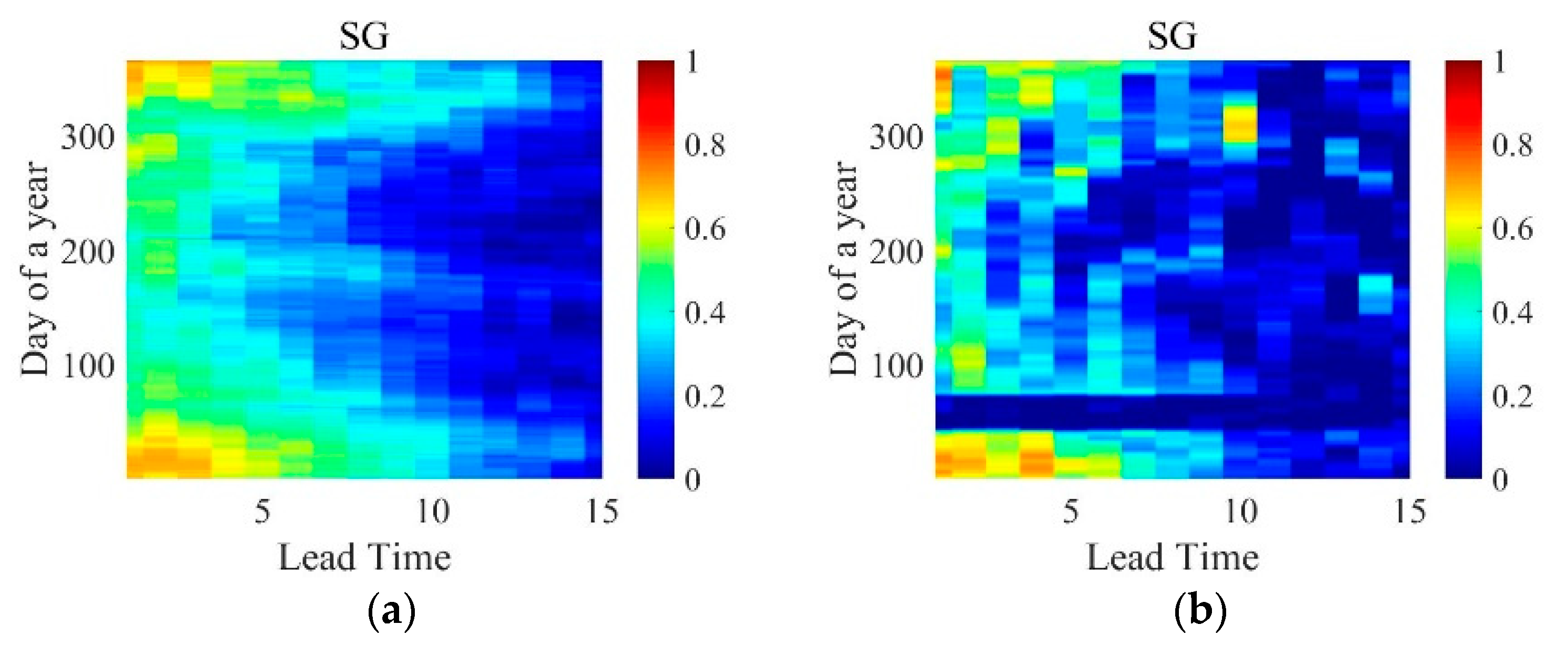
The ensemble means of the GEFS and CFSv2 forecasts are evaluated over the stations of the BJR based on observed precipitation. Taking the Shaoguan station as an example, Figure 3 displays the correlation coefficients of the observation and raw GEFS and CFSv2, respectively. The red color indicates high correlation, whereas the blue indicates low correlation. As shown in the figure, the results of GEFS are larger than those of CFSv2, which means the accuracy of GEFS is higher, and both accuracies are decreasing with the lead time. Besides, it can be found that both GEFS and CFSv2 have higher correlations in autumn and winter than in spring and summer, especially for the CFSv2, which performed nearly no prediction skills in the beginning of spring (Figure 3b). In addition, notable accuracy of GEFS forecasts can be recognized for the first few days (Figure 3a), and it can last about one week in the winter. A similar characteristic can also be detected in the results of CFSv2 but not remarkable.
4.2. Verification of the Processed Ensemble Forecasts
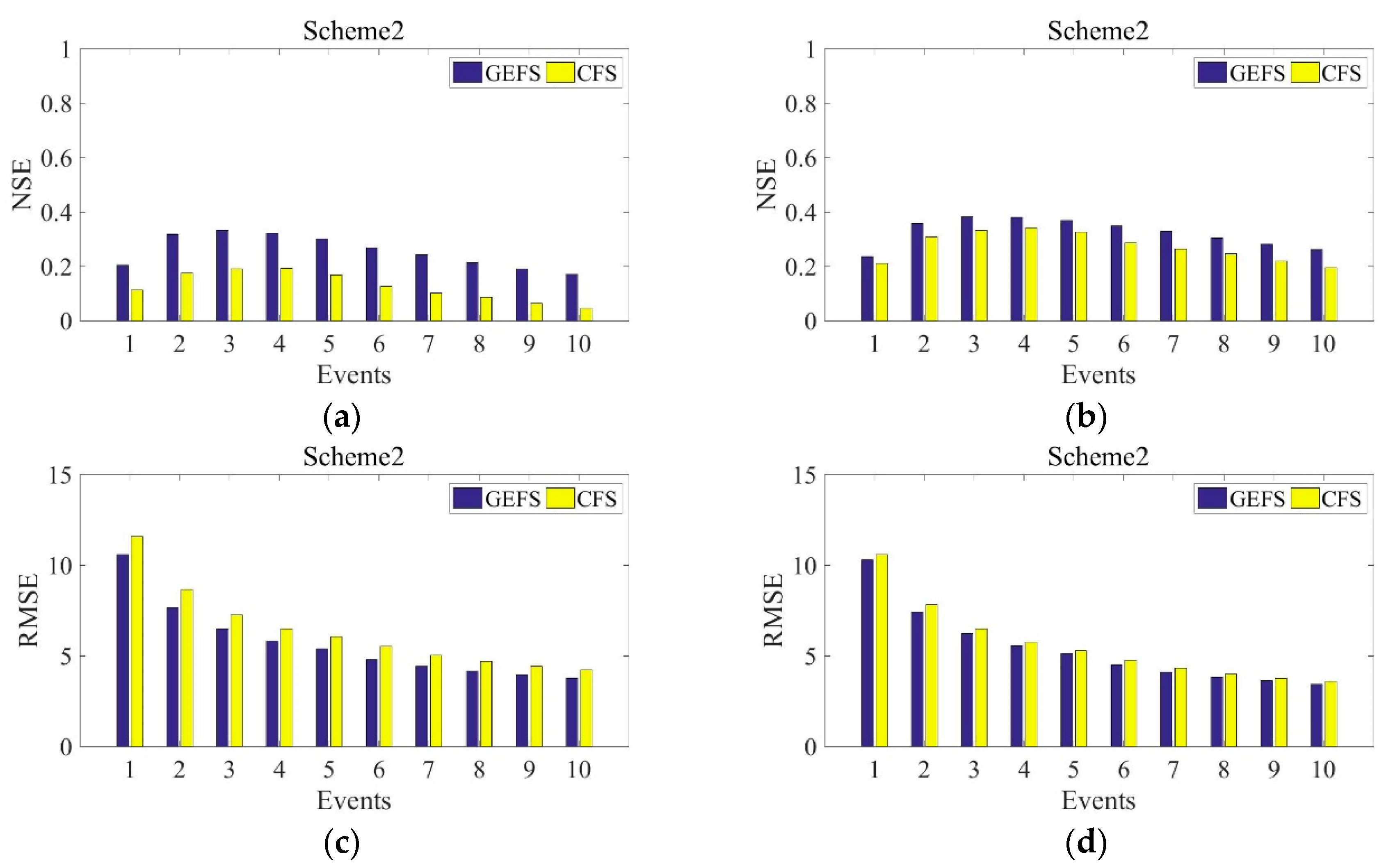
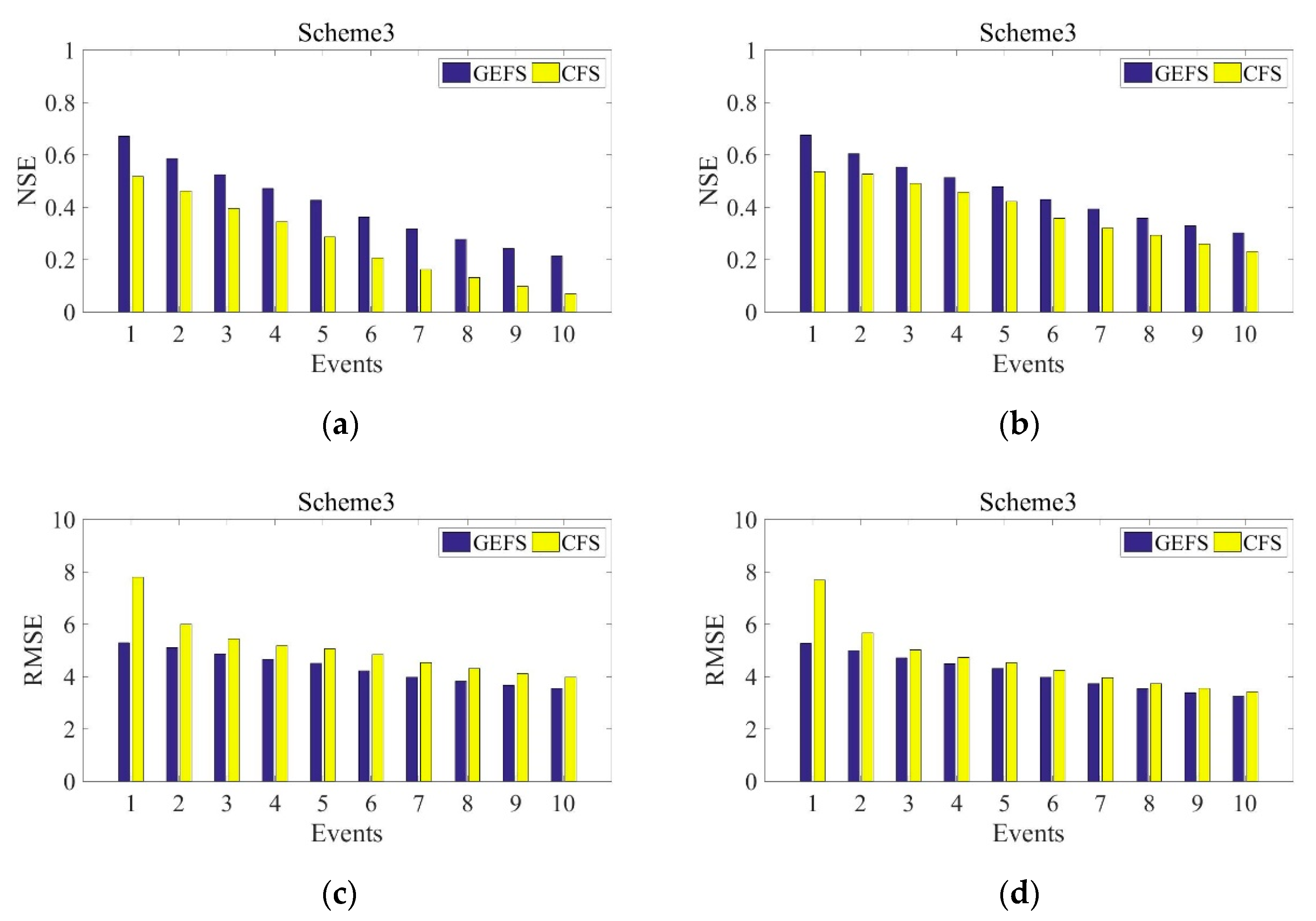
According to the analysis of raw GEFS and CFSv2, this study constructed four schemes to improve the accuracy by EPP. The designed schemes are displayed in Table 2 and the evaluation results by NSE and RMSE are displayed in Figure 4, Figure 5, Figure 6 and Figure 7. The left figures show the results of raw ensemble forecasts and the right ones show the post-processed forecasts by EPP.
Figure 4, Figure 5, Figure 6 and Figure 7 illustrate the evaluation results of Schemes 1–4, respectively, from which we can conclude that the schemes (Schemes 2–4) of cumulative forecast precipitation perform significantly better than the single-time step forecast, and the forecast precipitation of post-processed have higher accuracy compared to the raw forecasts. Moreover, the schemes (Schemes 3 and 4) considering observed information perform better than those that do not. The canonical events of composite time step designed for GEFS are effective to improve the forecast accuracy at a certain extent, whereas the events for CFSv2 are not performed ideally. The results of Scheme 1 show that CFSv2 is better than GEFS to some extent for single-time step forecast; however, it has little change under other schemes. This feature means that CFSv2 is concerned with climate information for a longer lead time and not very sensitive to the canonical events.
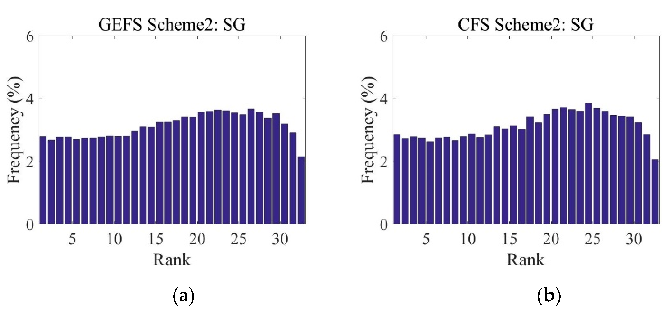
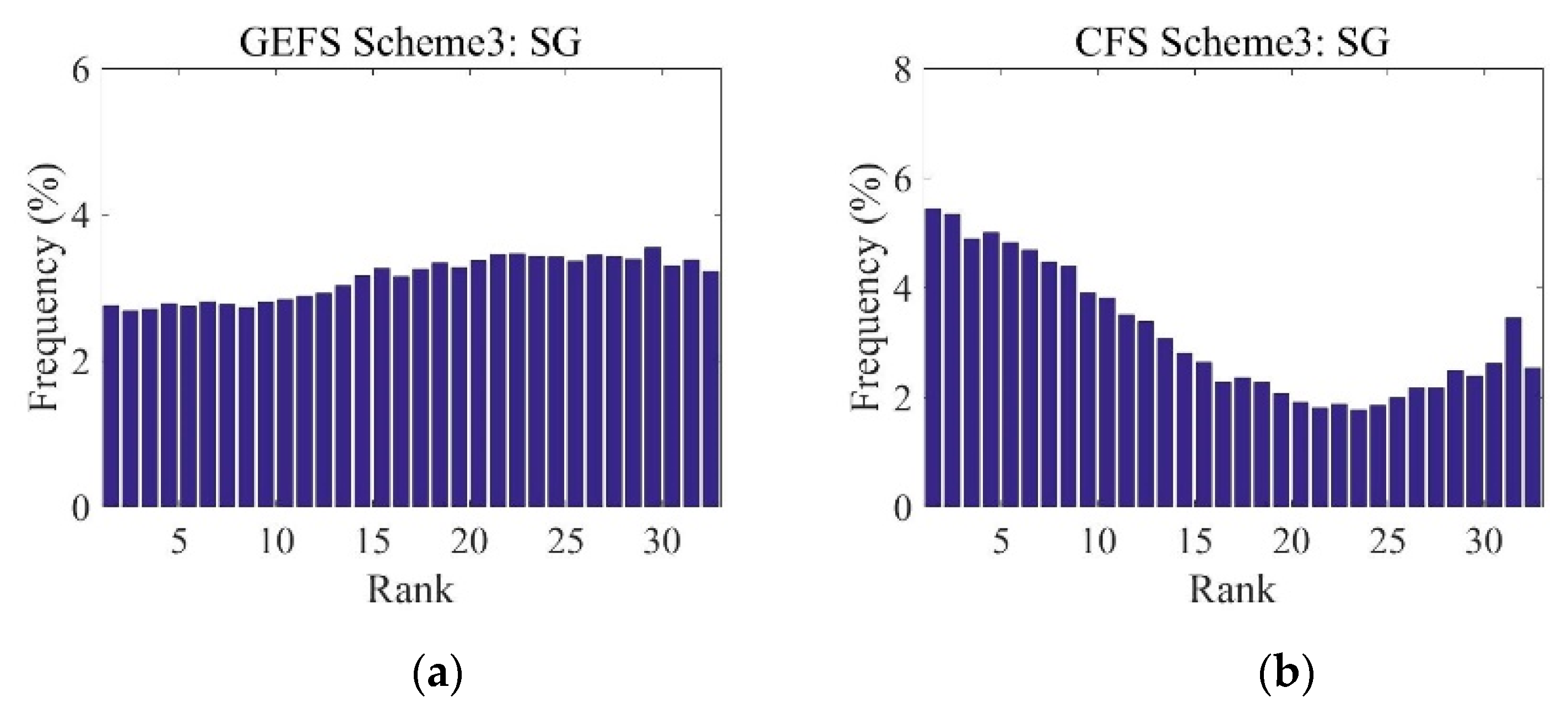
RH is used in this study to evaluate the reliability of ensemble distribution. The perfect forecast appears as the observation is evenly distributed in each level of the ensemble members. The RHs of Scheme 1 are not shown in this study since Figure 4 indicates that it cannot improve the forecast accuracy significantly. As mentioned above, Figure 8, Figure 9 and Figure 10 display the RHs of Shaoguan station under Schemes 2–4, respectively. The figures indicate that the schemes are designed properly to reduce error of raw GEFS and CFSv2. In comparison, Schemes 3 and 4 are better than Scheme 2 for GEFS, but they are not as good for CFSv2. The RHs of CFSv2 in Scheme 3 are right skewed U-shaped, which indicates that the range of ensemble members is narrower and most members are larger than the measured precipitation after post-processing. Scheme 4 shows a larger U-shaped differentiation, indicating that the post-processing results are further narrowed compared with Scheme 3.
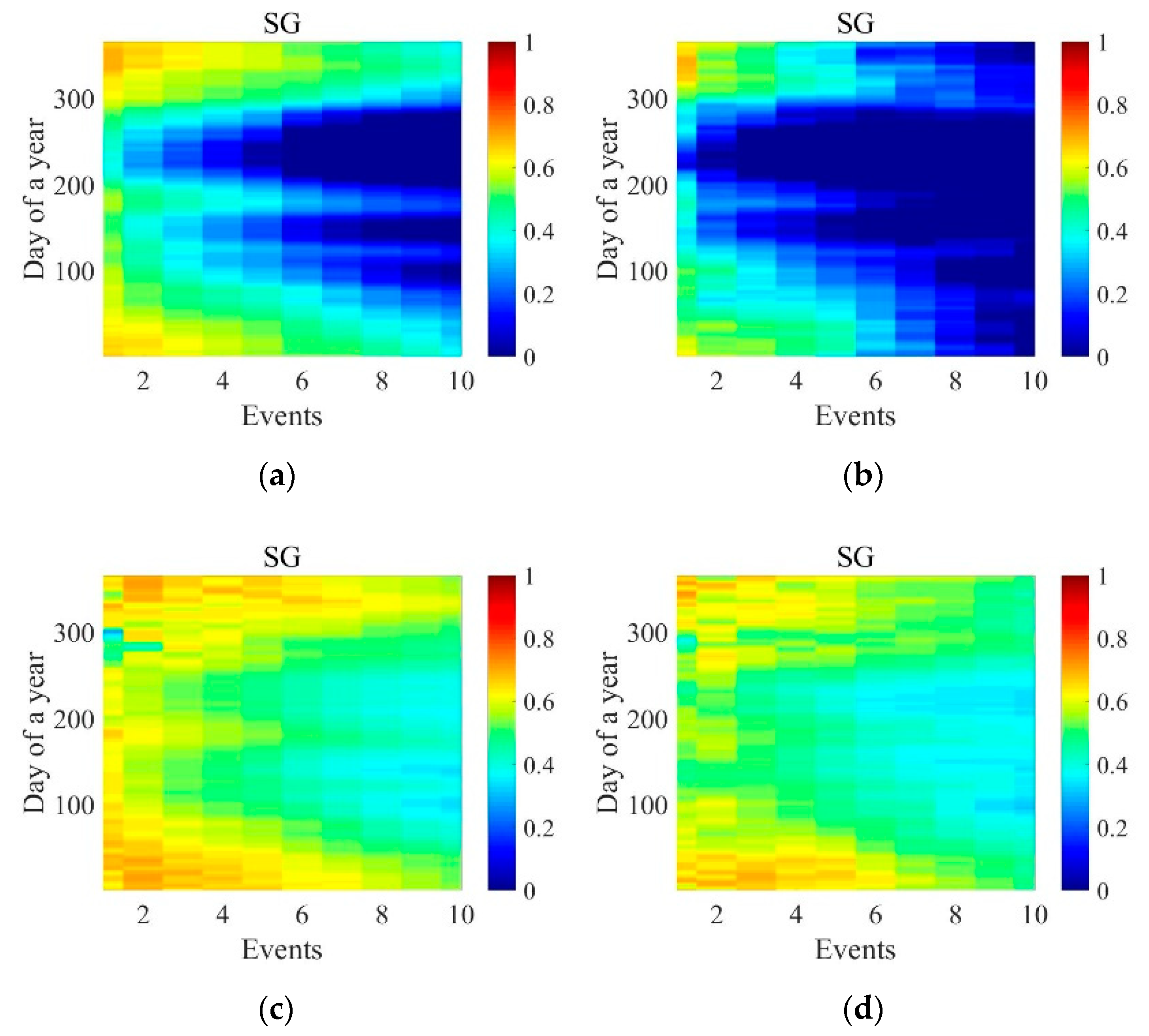
This study calculated the CRPSS of raw and post-processed ensemble forecast precipitation, respectively, to make a comparison. Only the results of Schemes 2 and 3 for Shaoguan station are shown in Figure 11 and Figure 12 considering the results of RH. The figures indicate that the raw forecasts have a lower CRPSS and differences exist in different stations. In addition, Scheme 2 shows that raw GEFS has higher CRPSS in cool seasons, and Fogang, which is lower latitude, has higher CRPSS than Shaoguan and Nanxiong in other seasons. This may be related to site location and climatic conditions; the annual precipitation of Fogang is larger than other stations. The CRPSS of CFSv2 indicates that it has almost no forecasting skills.
After post-processing, the CRPSS of GEFS and CFSv2 have become significantly larger, which means the EPP based on Schemes 2 and 3 can reduce the errors of ensemble forecast and improve the forecast accuracy. However, there are still many CRPSS of Event 1 in Scheme 2 which are lower than the normal value of other events, indicating that the precipitation samples of Event 1 are still not enough. It is necessary to take measures to increase precipitation samples for post-processing analysis. This problem does not exist in Scheme 3. On the whole, Scheme 3 would be the best one to improve the accuracy of ensemble forecast by EPP.
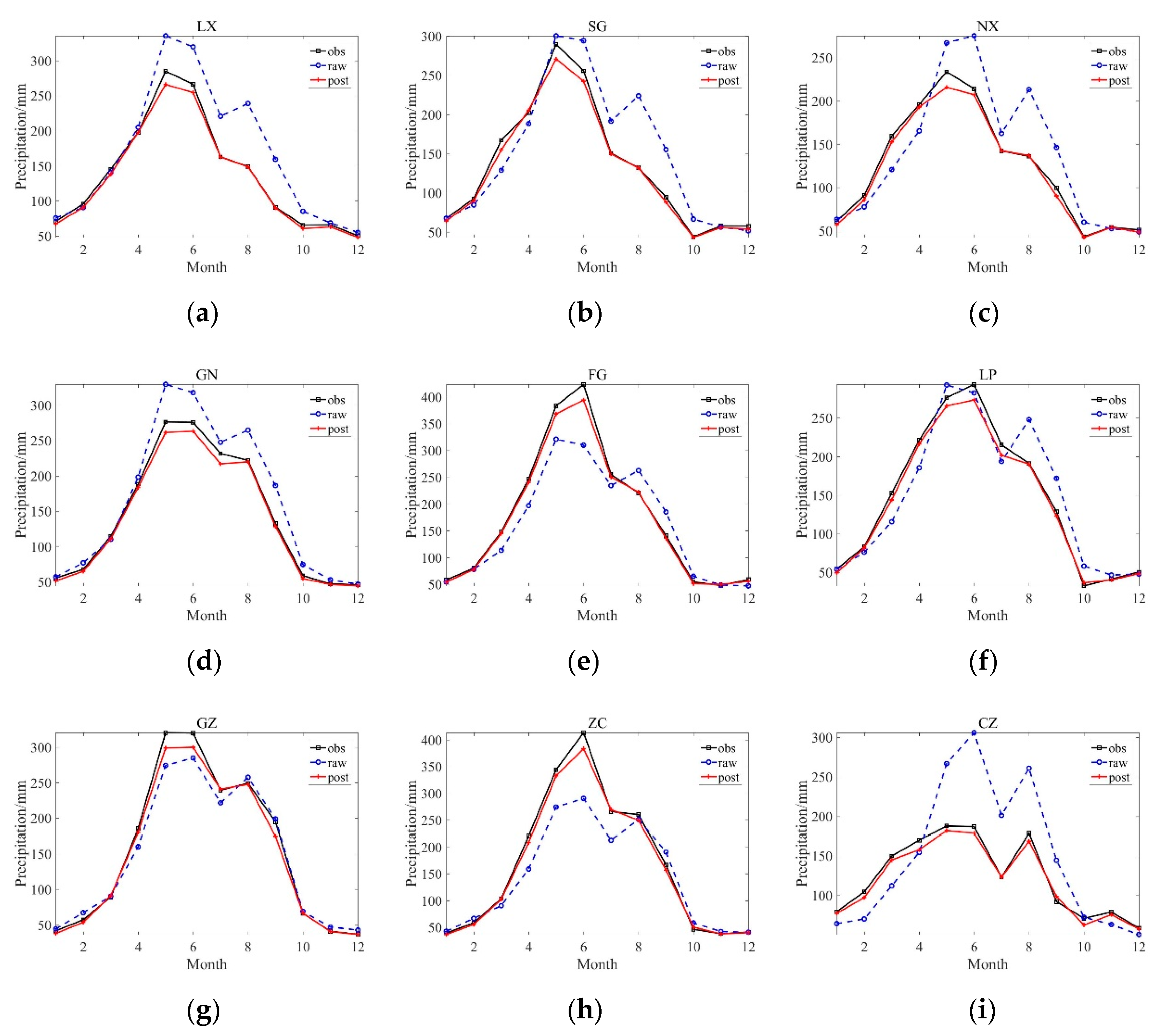
Figure 13 displays the annual average monthly precipitation of observed precipitation, raw GEFS forecast, and post-processed GEFS forecast, which are represented by black, blue, and red lines, respectively. We can conclude from the results in the figures that the raw forecast is more or less biased, but the new ensemble forecast results are close to the observed values after ensemble post-processing. In some areas where the raw ensemble forecast deviation is large, the optimization scheme in this paper can also greatly improve it.
4.3. Evaluation of Integrated Forecast Precipitation
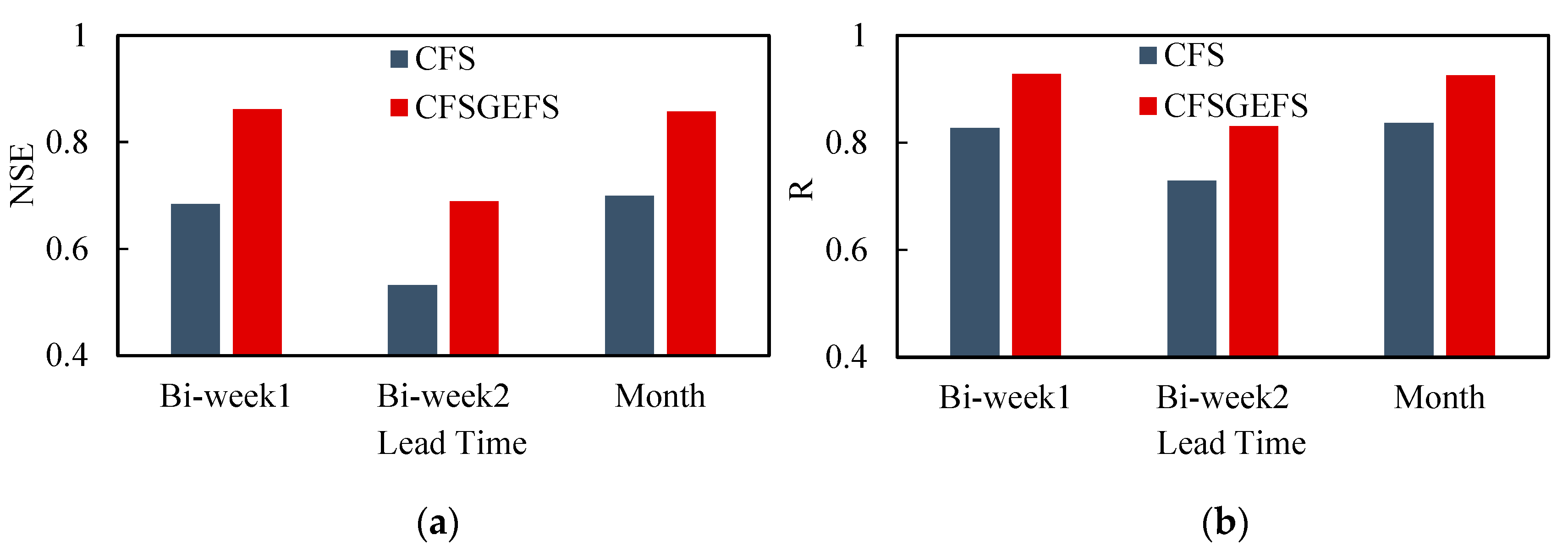
According to the above research, Scheme 3 has the best designed canonical events to reduce the deviation of ensemble forecast. In this section, the GEFS and CFSv2 are integrated into a new forecast series named CFSGEFS using EPP with the canonical events of Scheme 3 to test the performance of EPP in longer lead time, in which GEFS is selected for the former 15 days and CFSv2 for Days 16–30. We calculated the post-processed forecast precipitation of nine stations and turn them into surface rainfall of the BJR by the Thiessen polygons method to make comparison. The results are displayed in Figure 14, where CFS and CFSGEFS represent the evaluation results of post-processed CFSv2 and CFSGEFS in different time scales; Bi-Week 1 and Bi-Week 2 represent the former and latter two weeks of one month, respectively.
It can be concluded from the results in Figure 14 that the integrated forecast (CFSGEFS) performs better in weekly and monthly lead time comparing to the post-processed CFSv2. In addition, the results of Bi-Week 1 perform better than those of Bi-Week 2 since GEFS has higher forecast accuracy than CFSv2 in former days. This result indicates that the EPP can improve the forecast accuracy of CFSv2 in longer lead time significantly, but the integrated forecast precipitation improved by EPP would have better forecast accuracy and skills. The post-processed CFSGEFS precipitation can be used to improve the accuracy and reduce the uncertainty of hydrological prediction in long-term time scale.
5. Conclusions
Based on daily observed precipitation from meteorological stations of the BJR and GEFS and CFSv2 from NCEP, this study designed multiple schemes to correct deviations of ensemble forecast using EPP method and evaluated the accuracy of the results from multiple aspects. In addition, the best scheme was selected to integrate GEFS and CFSv2 to evaluate the forecast accuracy of long-term lead time. The processed results were evaluated by R, RMSE, NSE, RH, and CRPSS after many calculations, in which the former three indices were used to evaluate the ensemble mean and the latter indices were used to evaluate the ensemble distribution. We can conclude from the results that the raw forecasts of GEFS and CFSv2 contain more or less deviations and the EPP based on canonical events can improve their accuracy and give the deterministic forecast. The performance of results largely depends on the design of canonical events. In this study, Scheme 3 has been proven to be the optimal solution to improve forecast accuracy and reduce the uncertainty. However, the CFSv2 is not very sensitive to different designed schemes as it is concerned with climate information for a longer lead time. This study integrated the GEFS and CFSv2 by canonical events to try to improve the accuracy of long-time scale forecasting (e.g., weekly and monthly) considering the features of post-processed results. We found that the post-processing of integrated data can achieve better forecast results in longer time scales than that of CFSv2.
In summary, the EPP used in this study can improve the accuracy and reduce the uncertainty of ensemble forecasts significantly, and it can also be a helpful solution for long-term forecast of precipitation. These results would be very important for meteorological and hydrological ensemble prediction since they can be applied to many areas based on the global data and the precipitation forecast with higher precision can increase the accuracy and reduce the uncertainty of hydrological forecast, which plays a decisive role in preventing flood disasters. However, as the progress by EPP highly depends on the design of canonical events, the performance may vary in different regions. Therefore, the events should be redesigned when applied in other areas. In addition, the EPP can also be used to process the ensemble forecast of other elements from GEFS and CFSv2, which would be the following research and accompanied with a driving hydrological model in different time scales to evaluate the improving skills for hydrological forecasting.
Author Contributions
Conceptualization, X.C. (Xinchi Chen) and X.C. (Xiaohong Chen); methodology, X.C. (Xinchi Chen); formal analysis, X.C. (Xinchi Chen) and D.H.; investigation, X.C. (Xinchi Chen) and H.L.; data curation, X.C. (Xinchi Chen) and H.L.; writing—original draft preparation, X.C. (Xinchi Chen); writing—review and editing, X.C. (Xinchi Chen), X.C. (Xiaohong Chen) and D.H.; supervision, X.C. (Xinchi Chen) and X.C. (Xiaohong Chen); project administration, D.H.; and funding acquisition, D.H. and H.L. All authors have read and agreed to the published version of the manuscript.
Funding
This research was funded by the National Key Research and Development Program of China (No. 2016YFC0402604) and Water Science and Soft Science Research Project of Guangdong Province (No. 2018B020207004).
Acknowledgments
The authors would like to thank the National Centers for Environmental Prediction (NCEP) (https://www.ncep.noaa.gov/) for offering the Global Ensemble Forecast System (GEFS) and Climate Forecast System version 2 (CFSv2) data, and the China Meteorological Administration (http://data.cma.cn/) for the observed data used in this study. All support given by Aizhong Ye from Beijing Normal University is greatly appreciated for direction guidance and assistance.
Conflicts of Interest
The authors declare that there is no conflict of interests.
Appendix A

Table A1.
An example for the handling process of canonical events by Schaake Shuffle.
| Time (Year) | Observed Data | Canonical Events | Ascending Order of Forecast | Results | ||||||||
|---|---|---|---|---|---|---|---|---|---|---|---|---|
| Day 1 | Day 2 | Day 3 | Event 1 | Event 2 | K1 | K2 | Event 1 | Event 2 | Day 1 | Day 2 | Day 3 | |
| 2011 | 1.87 | 27.65 | 28.67 | (1.87 + 27.65)/2 = 14.76 | (1.87 + 27.65 + 28.67)/3 = 19.40 | 7 | 4 | 12.86(7) | 8.28(4) | 31.47 × 1.87/14.76 = 3.99 | 31.47 × 27.65/14.76 = 58.95 | 16.43 × 28.67/19.4 = 24.28 |
| 2012 | 18.2 | 10.97 | 29.76 | (18.23 + 10.97)/2 = 14.60 | (18.23 + 10.97 + 29.76)/3 = 19.65 | 4 | 10 | 18.51(4) | 10.94(10) | 30.07 × 18.23/14.6 = 37.54 | 30.07 × 10.97/14.6 = 22.59 | 22.77 × 29.76/19.65 = 34.49 |
| 2013 | 27.5 | 49.57 | 44.29 | (24.47 + 49.57)/2 = 38.52 | (24.47 + 49.57 + 44.29)/3 = 40.44 | 10 | 7 | 26.37(10) | 13.17(7) | 44.54 × 27.47/38.52 = 31.76 | 44.54 × 49.57/38.52 = 57.32 | 40.17 × 44.29/40.44 = 43.99 |
| 2014 | 3.21 | 14.75 | 4.6 | (3.21 + 14.75)/2 = 8.98 | (3.21 + 14.75 + 4.60)/3 = 7.52 | 2 | 1 | 30.07(2) | 16.43(1) | 18.51 × 3.21/8.98 = 6.62 | 18.51 × 14.75/8.98 = 30.4 | 8.28 × 4.6/7.52 = 5.06 |
| 2015 | 42.8 | 20.22 | 36.18 | (42.80 + 20.22)/2 = 31.51 | (42.80 + 20.22 + 36.18)/3 = 33.07 | 1 | 8 | 31.47(1) | 19.71(8) | 36.68 × 42.8/31.51 = 49.83 | 36.68 × 20.22/31.51 = 23.54 | 25.29 × 36.18/33.07 = 27.67 |
| 2016 | 32.2 | 38.77 | 47.98 | (32.15 + 38.77)/2 = 35.46 | (32.15 + 38.77 + 47.98)/3 = 39.64 | 8 | 2 | 32.88(8) | 22.77(2) | 43.62 × 32.15/35.46 = 39.55 | 43.62 × 38.77/35.46 = 47.69 | 35.21 × 47.98/39.64 = 42.62 |
| 2017 | 2.91 | 12.74 | 25.99 | (2.91 + 12.74)/2 = 7.83 | (2.91 + 12.74 + 25.99)/3 = 13.88 | 5 | 5 | 36.68(5) | 25.29(5) | 12.86 × 2.91/7.83 = 4.78 | 12.86 × 12.74/7.83 = 20.92 | 13.17 × 25.99/13.88 = 24.66 |
| 2018 | 38.5 | 3.82 | 16.28 | (38.51 + 3.82)/2 = 21.17 | (38.51 + 3.82 + 16.28)/3 = 19.54 | 6 | 6 | 43.62(6) | 35.21(6) | 32.88 × 38.51/21.17 = 59.81 | 32.88 × 3.82/21.17 = 5.93 | 19.71 × 16.28/19.54 = 16.42 |
| 2019 | 47.1 | 41.78 | 43.01 | (47.09 + 41.78)/2 = 44.44 | (47.09 + 41.78 + 43.01)/3 = 43.96 | 3 | 3 | 44.54(3) | 40.17(3) | 46.45 × 47.09/44.44 = 49.22 | 46.45 × 41.78/44.44 = 43.67 | 41.04 × 43.01/43.96 = 40.15 |
| 2020 | 11.4 | 17.41 | 2.47 | (11.39 + 17.41)/2 = 14.40 | (11.39 + 17.41 + 2.47)/3 = 10.42 | 9 | 9 | 46.45(9) | 41.04(9) | 26.37 × 11.39/14.4 = 20.86 | 26.37 × 17.41/14.4 = 31.88 | 10.94 × 2.47/10.42 = 2.59 |
The observed and forecast data are randomly sampled between 1 and 50.
References
- Hirabayashi, Y.; Mahendran, R.; Koirala, S.; Konoshima, L.; Yamazaki, D.; Watanabe, S.; Kim, H.; Kanae, S. Global flood risk under climate change. Nat. Clim. Chang. 2013, 3, 816–821. [Google Scholar] [CrossRef]
- Chen, X.; Zhang, L.; Gippel, C.J.; Shan, L.; Chen, S.; Yang, W. Uncertainty of flood forecasting based on radar rainfall data assimilation. Adv. Meteorol. 2016, 2016. [Google Scholar] [CrossRef] [Green Version]
- Zanchetta, A.; Coulibaly, P. Recent advances in real-time pluvial flash flood forecasting. Water 2020, 12, 570. [Google Scholar] [CrossRef] [Green Version]
- Shahrban, M.; Walker, J.P.; Wang, Q.J.; Seed, A.; Steinle, P. An evaluation of numerical weather prediction based rainfall forecasts. Hydrol. Sci. J. 2016, 61, 2704–2717. [Google Scholar] [CrossRef] [Green Version]
- Wang, G.; Yang, J.; Wang, D.; Liu, L. A quantitative comparison of precipitation forecasts between the storm-scale numerical weather prediction model and auto-nowcast system in Jiangsu, China. Atmos. Res. 2016, 181, 1–11. [Google Scholar] [CrossRef] [Green Version]
- Shrestha, D.L.; Robertson, D.E.; Wang, Q.J.; Pagano, T.C.; Hapuarachchi, H.A.P. Evaluation of numerical weather prediction model precipitation forecasts for short-term streamflow forecasting purpose. Hydrol. Earth Syst. Sci. 2013, 17, 1913–1931. [Google Scholar] [CrossRef] [Green Version]
- Luitel, B.; Villarini, G.; Vecchi, G.A. Verification of the skill of numerical weather prediction models in forecasting rainfall from U.S. landfalling tropical cyclones. J. Hydrol. 2018, 556, 1026–1037. [Google Scholar] [CrossRef]
- Ran, Q.; Fu, W.; Liu, Y.; Li, T.; Shi, K.; Sivakumar, B. Evaluation of quantitative precipitation predictions by ECMWF, CMA, and UKMO for flood forecasting: Application to two basins in china. Nat. Hazards Rev. 2018, 19, 5018003. [Google Scholar] [CrossRef] [Green Version]
- Duan, M.; Ma, J.; Wang, P. Preliminary comparison of the CMA, ECMWF, NCEP, and JMA ensemble prediction systems. Acta Meteorol. Sin. 2012, 26, 26–40. [Google Scholar] [CrossRef]
- Su, X.; Yuan, H.; Zhu, Y.; Luo, Y.; Wang, Y. Evaluation of TIGGE ensemble predictions of Northern Hemisphere summer precipitation during 2008-2012. J. Geophys. Res. Atmos. 2014, 119, 7292–7310. [Google Scholar] [CrossRef]
- Zhou, X.; Zhu, Y.; Hou, D.; Luo, Y.; Peng, J.; Wobus, R. Performance of the New NCEP global ensemble forecast system in a parallel experiment. Weather Forecast. 2017, 32, 1989–2004. [Google Scholar] [CrossRef]
- Saha, S.; Moorthi, S.; Wu, X.; Wang, J.; Nadiga, S.; Tripp, P.; Behringer, D.; Hou, Y.; Chuang, H.; Iredell, M.; et al. The NCEP climate forecast system version 2. J. Clim. 2014, 27, 2185–2208. [Google Scholar] [CrossRef]
- Bougeault, P.; Toth, Z.; Bishop, C.; Brown, B.; Burridge, D.; Chen, D.H.; Ebert, B.; Fuentes, M.; Hamill, T.M.; Mylne, K.; et al. The THORPEX interactive grand global ensemble. Bull. Am. Meteorol. Soc. 2010, 91, 1059–1072. [Google Scholar] [CrossRef]
- Liu, Y.; Duan, Q.; Zhao, L.; Ye, A.; Tao, Y.; Miao, C.; Mu, X.; Schaake, J.C. Evaluating the predictive skill of post-processed NCEP GFS ensemble precipitation forecasts in China’s Huai river basin. Hydrol. Process. 2013, 27, 57–74. [Google Scholar] [CrossRef]
- Klein, W.H.; Lewis, B.M.; Enger, I. Objective prediction of five-day mean temperatures during winter. J. Meteorol. 1959, 16, 672–682. [Google Scholar] [CrossRef] [Green Version]
- Glahn, H.R.; Lowry, D.A. The use of model output statistics (MOS) in objective weather forecasting. J. Appl. Meteorol. 1972, 11, 1203–1211. [Google Scholar] [CrossRef] [Green Version]
- Hamill, T.M. Interpretation of rank histograms for verifying ensemble forecasts. Mon. Weather Rev. 2001, 129, 550–560. [Google Scholar] [CrossRef]
- Reggiani, P.; Weerts, A.H. Probabilistic quantitative precipitation forecast for flood prediction: An application. J. Hydrometeorol. 2008, 9, 76–95. [Google Scholar] [CrossRef]
- Piani, C.; Haerter, J.O.; Coppola, E. Statistical bias correction for daily precipitation in regional climate models over Europe. Theor. Appl. Climatol. 2010, 99, 187–192. [Google Scholar] [CrossRef] [Green Version]
- Schaake, J.; Demargne, J.; Hartman, R.; Mullusky, M.; Welles, E.; Wu, L.; Herr, H.; Fan, X.; Seo, D. Precipitation and temperature ensemble forecasts from single-value forecasts. Hydrol. Earth Syst. Sci. Discuss. 2007, 4, 655–717. [Google Scholar] [CrossRef]
- Wu, L.; Seo, D.; Demargne, J.; Brown, J.; Cong, S.; Schaake, J. Generation of ensemble precipitation forecast from single-valued quantitative precipitation forecast for hydrologic ensemble prediction. J. Hydrol. 2011, 399, 281–298. [Google Scholar] [CrossRef]
- Verkade, J.; Brown, J.; Reggiani, P.; Weerts, A. Post-processing ECMWF precipitation and temperature ensemble reforecasts for operational hydrologic forecasting at various spatial scales. J. Hydrol. 2013, 501, 73–91. [Google Scholar] [CrossRef]
- Zhu, Y.; Luo, Y. Precipitation calibration based on frequency matching method. Weather Forecast. 2014, 30, 1109–1124. [Google Scholar] [CrossRef]
- Hashino, T.; Bradley, A.; Schwartz, S. Evaluation of bias-correction methods for ensemble streamflow volume forecasts. Hydrol. Earth Syst. Sci. Discuss. 2007, 3, 939–950. [Google Scholar] [CrossRef] [Green Version]
- Wood, A.W.; Lettenmaier, D.P. An ensemble approach for attribution of hydrologic prediction uncertainty. Geophys. Res. Lett. 2008, 35. [Google Scholar] [CrossRef] [Green Version]
- Li, W.; Duan, Q.; Ye, A.; Gong, W.; Di, Z. A review on statistical postprocessing methods for hydrometeorological ensemble forecasting: Statistical postprocessing methods. Wiley Interdiscip. Rev. Water 2017, 1–24. [Google Scholar] [CrossRef]
- Zhao, T.; Bennett, J.C.; Wang, Q.J.; Schepen, A.; Wood, A.W.; Robertson, D.E.; Ramos, M. How suitable is quantile mapping for postprocessing GCM precipitation forecasts? J. Clim. 2017, 30, 3185–3196. [Google Scholar] [CrossRef]
- Ye, A.; Duan, Q.; Yuan, X.; Wood, E.F.; Schaake, J. Hydrologic post-processing of MOPEX streamflow simulations. J. Hydrol. 2014, 508, 147–156. [Google Scholar] [CrossRef]
- Krzysztofowicz, R.; Maranzano, C. Bayesian processor of output for probabilistic quantitative precipitation forecasting. AGU Spring Meet. Abstr. 2006, 31, 1–53. [Google Scholar]
- Clark, M.; Gangopadhyay, S.; Hay, L.; Rajagopalan, B.; Wilby, R. The Schaake Shuffle: A method for reconstructing space–time variability in forecasted precipitation and temperature fields. J. Hydrometeorol. 2004, 5, 243–262. [Google Scholar] [CrossRef] [Green Version]
- Liu, J.; Bray, M.; Han, D. A study on WRF radar data assimilation for hydrological rainfall prediction. Hydrol. Earth Syst. Sci. 2013, 17, 3095–3110. [Google Scholar] [CrossRef] [Green Version]
- Tao, Y.; Duan, Q.; Ye, A.; Gong, W.; Di, Z.; Xiao, M.; Hsu, K. An evaluation of post-processed TIGGE multimodel ensemble precipitation forecast in the Huai river basin. J. Hydrol. 2014, 519, 2890–2905. [Google Scholar] [CrossRef] [Green Version]
- Toth, Z.; Kalnay, E. Ensemble Forecasting at NCEP and the Breeding Method. Mon. Weather Rev. 1997, 125, 3297–3319. [Google Scholar] [CrossRef]
- Lorenz, E.N. Deterministic nonperiodic flow. J. Atmos. Sci. 1963, 20, 130–141. [Google Scholar] [CrossRef] [Green Version]
- Ye, A.; Deng, X.; Ma, F.; Duan, Q.; Zhou, Z.; Du, C. Integrating weather and climate predictions for seamless hydrologic ensemble forecasting: A case study in the Yalong River basin. J. Hydrol. 2017, 547, 196–207. [Google Scholar] [CrossRef]
- Bröcker, J. On reliability analysis of multi-categorical forecasts. Nonlinear Process. Geophys. 2008, 15, 661–673. [Google Scholar] [CrossRef] [Green Version]
- Bröcker, J.; Bouallègue, B.Z. Stratified rank histograms for ensemble forecast verification under serial dependence. Q. J. R. Meteorol. Soc. 2020, 146, 1976–1990. [Google Scholar] [CrossRef]
- McCollor, D.; Stull, R. Evaluation of probabilistic medium-range temperature forecasts from the North American ensemble forecast system. Weather Forecast. 2009, 24, 3–17. [Google Scholar] [CrossRef] [Green Version]
- Hersbach, H. Decomposition of the continuous ranked probability score for ensemble prediction systems. Weather Forecast. 2000, 15, 559–570. [Google Scholar] [CrossRef]
Figure 1.
The topographic map of BJR and average annual precipitation of meteorological stations.

Figure 2.
Annual precipitation over the BJR: the black dotted line with circles represents the precipitation over the whole area, the blue line indicates the five-year moving average, and the red line represents the linear trend.
Figure 2.
Annual precipitation over the BJR: the black dotted line with circles represents the precipitation over the whole area, the blue line indicates the five-year moving average, and the red line represents the linear trend.

Figure 3.
The correlation coefficients of observation and raw forecast data: (a) GEFS; and (b) CFSv2.
Figure 3.
The correlation coefficients of observation and raw forecast data: (a) GEFS; and (b) CFSv2.

Figure 4.
The evaluation results of Scheme 1: (a) the NSE of raw forecasts; (b) the NSE of post-processed forecasts; (c) the RMSE of raw forecasts; and (d) the RMSE of post-processed forecasts.
Figure 4.
The evaluation results of Scheme 1: (a) the NSE of raw forecasts; (b) the NSE of post-processed forecasts; (c) the RMSE of raw forecasts; and (d) the RMSE of post-processed forecasts.

Figure 5.
The evaluation results of Scheme 2: (a) the NSE of raw forecasts; (b) the NSE of post-processed forecasts; (c) the RMSE of raw forecasts; and (d) the RMSE of post-processed forecasts.
Figure 5.
The evaluation results of Scheme 2: (a) the NSE of raw forecasts; (b) the NSE of post-processed forecasts; (c) the RMSE of raw forecasts; and (d) the RMSE of post-processed forecasts.

Figure 6.
The evaluation results of Scheme 3: (a) the NSE of raw forecasts; (b) the NSE of post-processed forecasts; (c) the RMSE of raw forecasts; and (d) the RMSE of post-processed forecasts.
Figure 6.
The evaluation results of Scheme 3: (a) the NSE of raw forecasts; (b) the NSE of post-processed forecasts; (c) the RMSE of raw forecasts; and (d) the RMSE of post-processed forecasts.

Figure 7.
The evaluation results of Scheme 4: (a) the NSE of raw forecasts; (b) the NSE of post-processed forecasts; (c) the RMSE of raw forecasts; and (d) the RMSE of post-processed forecasts.
Figure 7.
The evaluation results of Scheme 4: (a) the NSE of raw forecasts; (b) the NSE of post-processed forecasts; (c) the RMSE of raw forecasts; and (d) the RMSE of post-processed forecasts.

Figure 8.
RHs of Shaoguan under the Scheme 2: (a) GEFS; and (b) CFSv2.

Figure 9.
RHs of Shaoguan under the Scheme 3: (a) GEFS; and (b) CFSv2.

Figure 10.
RHs of Shaoguan under the Scheme 4: (a) GEFS; and (b) CFSv2.

Figure 11.
The CRPSS results of Scheme 2 for Shaoguan: (a) raw GEFS; (b) raw CFSv2; (c) post-processed GEFS; and (d) post-processed CFSv2.
Figure 11.
The CRPSS results of Scheme 2 for Shaoguan: (a) raw GEFS; (b) raw CFSv2; (c) post-processed GEFS; and (d) post-processed CFSv2.

Figure 12.
The CRPSS results of Scheme 3 for Shaoguan: (a) raw GEFS; (b) raw CFSv2; (c) post-processed GEFS; and (d) post-processed CFSv2.
Figure 12.
The CRPSS results of Scheme 3 for Shaoguan: (a) raw GEFS; (b) raw CFSv2; (c) post-processed GEFS; and (d) post-processed CFSv2.

Figure 13.
Comparison of annual average monthly precipitation before and after post-processing of GEFS with observed data: (a) Lianxian; (b) Shaoguan; (c) Nanxiong; (d) Guangning; (e) Fogang; (f) Lianping; (g) Guangzhou; (h) Zengcheng; and (i) Chenzhou.
Figure 13.
Comparison of annual average monthly precipitation before and after post-processing of GEFS with observed data: (a) Lianxian; (b) Shaoguan; (c) Nanxiong; (d) Guangning; (e) Fogang; (f) Lianping; (g) Guangzhou; (h) Zengcheng; and (i) Chenzhou.

Figure 14.
The evaluation results of integrated forecast precipitation in weekly and monthly lead time: (a) the result of NSE; and (b) the result of R.
Figure 14.
The evaluation results of integrated forecast precipitation in weekly and monthly lead time: (a) the result of NSE; and (b) the result of R.

Table 1.
Annual precipitation of the meteorological stations.
| Name | Abbreviation | Mean (mm) | Max (mm) | Min (mm) |
|---|---|---|---|---|
| Nanxiong | NX | 1482.75 | 1966 | 1040.5 |
| Lianxian | LX | 1645.97 | 2350.3 | 1081 |
| Shaoguan | SG | 1610.97 | 2132.1 | 1169.3 |
| Fogang | FG | 2118.96 | 2765.9 | 1183.8 |
| Lianping | LP | 1740.33 | 2396.9 | 1168 |
| Guangning | GN | 1716.82 | 2096.6 | 1102.8 |
| Guangzhou | GZ | 1841.46 | 2678.9 | 1239.5 |
| Zengcheng | ZC | 1998.25 | 2702.5 | 1224.9 |
| Chenzhou | CZ | 1440.6 | 2209.4 | 982.7 |
Table 2.
Designed schemes of canonical events.
| Event 1 | Event 2 | Event 3 | Event 4 | Event 5 | Event 6 | Event 7 | Event 8 | Event 9 | Event 10 | ||
|---|---|---|---|---|---|---|---|---|---|---|---|
| Scheme 1 | Start | 1 | 2 | 3 | 4 | 5 | 6 | 8 | 10 | 12 | 14 |
| End | 1 | 2 | 3 | 4 | 5 | 7 | 9 | 11 | 13 | 15 | |
| Scheme 2 | Start | 1 | 1 | 1 | 1 | 1 | 1 | 1 | 1 | 1 | 1 |
| End | 1 | 2 | 3 | 4 | 5 | 7 | 9 | 11 | 13 | 15 | |
| Scheme 3 | Start | −1 | −1 | −1 | −1 | −1 | −1 | −1 | −1 | −1 | −1 |
| End | 1 | 2 | 3 | 4 | 5 | 7 | 9 | 11 | 13 | 15 | |
| Scheme 4 | Start | −3 | −3 | −3 | −3 | −3 | −3 | −3 | −3 | −3 | −3 |
| End | 1 | 2 | 3 | 4 | 5 | 7 | 9 | 11 | 13 | 15 | |
© 2020 by the authors. Licensee MDPI, Basel, Switzerland. This article is an open access article distributed under the terms and conditions of the Creative Commons Attribution (CC BY) license (http://creativecommons.org/licenses/by/4.0/).
Share and Cite
MDPI and ACS Style
Chen, X.; Chen, X.; Huang, D.; Liu, H. Post-Processing and Evaluation of Precipitation Ensemble Forecast under Multiple Schemes in Beijiang River Basin. Water 2020, 12, 2631. https://doi.org/10.3390/w12092631
AMA Style
Chen X, Chen X, Huang D, Liu H. Post-Processing and Evaluation of Precipitation Ensemble Forecast under Multiple Schemes in Beijiang River Basin. Water. 2020; 12(9):2631. https://doi.org/10.3390/w12092631
Chicago/Turabian StyleChen, Xinchi, Xiaohong Chen, Dong Huang, and Huamei Liu. 2020. "Post-Processing and Evaluation of Precipitation Ensemble Forecast under Multiple Schemes in Beijiang River Basin" Water 12, no. 9: 2631. https://doi.org/10.3390/w12092631
Note that from the first issue of 2016, this journal uses article numbers instead of page numbers. See further details here.