Climate-Biome Envelope Shifts Create Enormous Challenges and Novel Opportunities for Conservation

Abstract

Research Highlights: We modeled climate-biome envelopes at high resolution in the Western Great Lakes Region for recent and future time-periods. The projected biome shifts, in conjunction with heterogeneous distribution of protected land, may create both great challenges for conservation of particular ecosystems and novel conservation opportunities. Background and Objectives: Climate change this century will affect the distribution and relative abundance of ecological communities against a mostly static background of protected land. We developed a climate-biome envelope model using a priori climate-vegetation relationships for the Western Great Lakes Region (Minnesota, Wisconsin and Michigan USA and adjacent Ontario, Canada) to predict potential biomes and ecotones—boreal forest, mixed forest, temperate forest, prairie–forest border, and prairie—for a recent climate normal period (1979–2013) and future conditions (2061–2080). Materials and Methods: We analyzed six scenarios, two representative concentration pathways (RCP)—4.5 and 8.5, and three global climate models to represent cool, average, and warm scenarios to predict climate-biome envelopes for 2061–2080. To assess implications of the changes for conservation, we analyzed the amount of land with climate suited for each of the biomes and ecotones both region-wide and within protected areas, under current and future conditions. Results: Recent biome boundaries were accurately represented by the climate-biome envelope model. The modeled future conditions show at least a 96% loss in areas suitable for the boreal and mixed forest from the region, but likely gains in areas suitable for temperate forest, prairie–forest border, and prairie. The analysis also showed that protected areas in the region will most likely lose most or all of the area, 18,692 km², currently climatically suitable for boreal forest. This would represent an enormous conservation loss. However, conversely, the area climatically suitable for prairie and prairie–forest border within protected areas would increase up to 12.5 times the currently suitable 1775 km². Conclusions: These results suggest that retaining boreal forest in potential refugia where it currently exists and facilitating transition of some forests to prairie, oak savanna, and temperate forest should both be conservation priorities in the northern part of the region.

1. Introduction

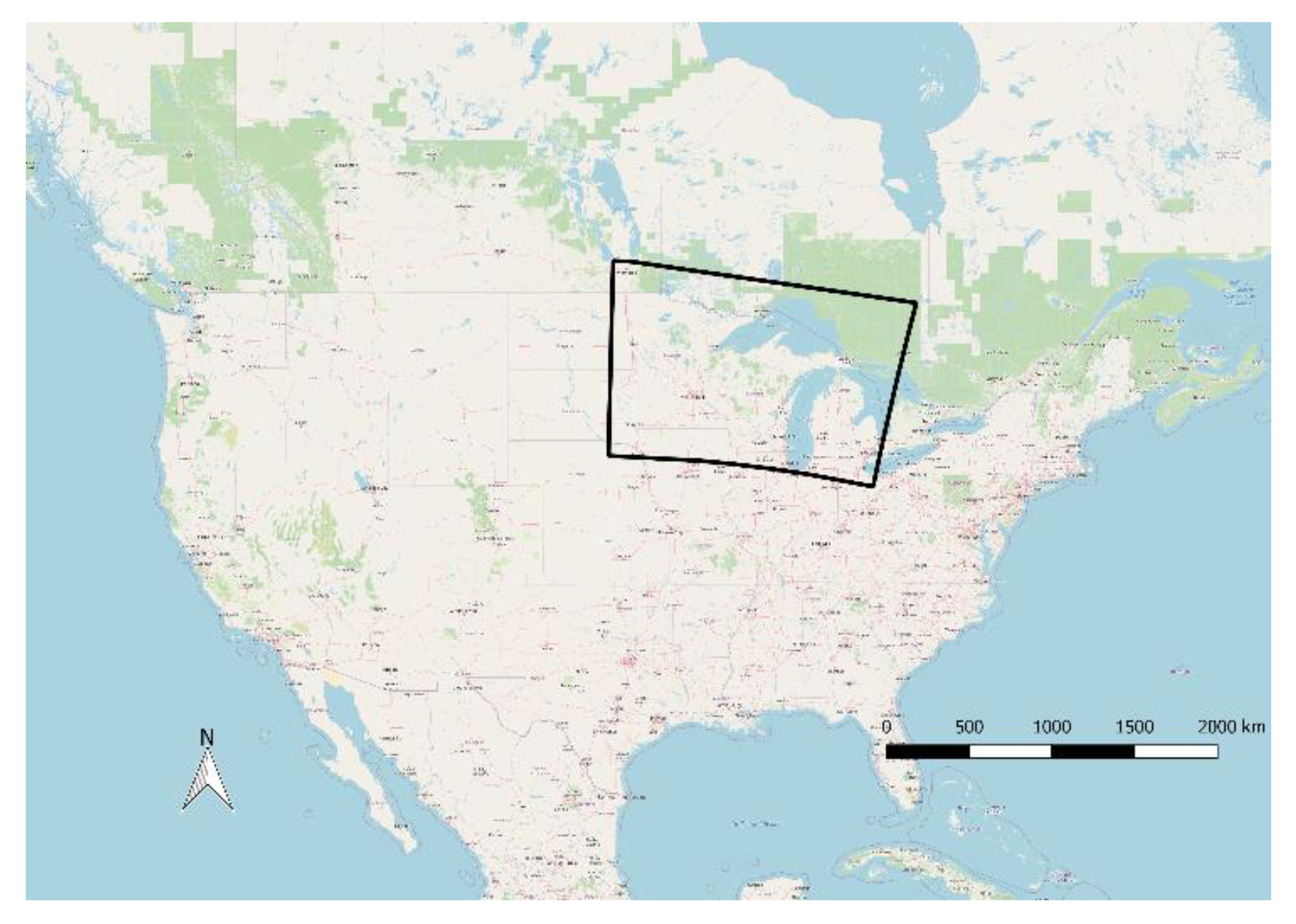
The Western Great Lakes Region in midcontinental North America (Minnesota, Wisconsin, and Michigan USA and adjacent Ontario, Canada—shown in Figure 1), is one of two interior continental regions of the world where prairie, boreal, and temperate biomes meet. The northwestern part of the region is host to the Quetico-Superior Ecosystem (QSE), a land of boreal and Laurentian (boreal and temperate) mixed forests and thousands of glacier-carved lakes on the ancient bedrock of the Canadian Shield. The QSE includes Voyageur’s National Park and the Boundary Waters Canoe Area Wilderness (BWCAW) in the U.S. and Quetico Provincial Park (QPP) in Canada—the latter two contain one of the largest tracts of primeval unlogged forest in eastern North America [1]. Climate change threatens the continued existence of boreal species integral to the plant communities of the QSE, and more broadly, the boreal biome in the region, due to warmer temperatures and periodically drier soils [2,3,4,5]. Conversely, oak savanna and prairie, once ubiquitous in the southwest part of the region have been nearly eliminated by land use conversion, mostly to agriculture [6,7]. Climate change is of further concern here because of the limited ability of prairie species on small remnants embedded in vast agricultural landscapes to respond to a warming climate with rapid migration [2].

Temperate forests lie generally between the region’s prairies and boreal forest, resulting in boreal-temperate forest and prairie–forest ecotones subject to shifts with climate change. Although many factors determine vegetation composition in a given location and time including geology and geomorphic processes, soil, landform, anthropogenic land management, legacy, and disturbance, climate is a driving factor at the biome scale [9,10], and found to be most important for the thresholds in this region of study. The southern extent in this region of several boreal conifers-black spruce (Picea mariana (Mill.) Britton, Sterns & Poggenb.), white spruce (Picea glauca (Moench) Voss), and balsam fir (Abies balsamea (L.) Mill.) is mainly controlled by mean summer temperature [4,11]. Depending on climate–change scenario, summer temperatures in this region will likely rise 2.0 °C to 5.5 °C by 2080 from 18.7 °C in 1979–2013 [12]. Temperate species such as sugar maple (Acer saccharum Marshall), American basswood (Tilia americana L.), and northern red oak (Quercus rubra L.) may compete better within the boreal-temperate ecotone and expand their ranges northward with the help of higher temperatures [11]. The potentially diminished ability of boreal species to compete may extirpate most of the boreal forest and the boreal component of mixed forests [2]. The prairie–forest border, too, is expected to shift northeast due to climate change and other complex factors [3]. Climatic moisture balance, as a surrogate for or possibly in conjunction with fire, largely determines the position of the prairie–forest border in North America—areas with positive balances (more annual precipitation than potential evapotranspiration) support forests [13,14,15]. As the climate warms, higher temperatures, especially during summer, will drive additional evaporation and transpiration, and although mean annual precipitation may increase slightly, it is expected to decrease during the summer months. Together, these effects will create a drier climate, driving the northeastward migration of the prairie–forest border. The changing distribution of biomes against a heterogeneous and relatively static arrangement of protected land may have critical impacts on conservation efforts for two reasons. First, vegetation of the Western Great Lakes Region is particularly susceptible to climate change for several reasons: a large number of species at the trailing edge of their ranges, the presence of biome ecotones, a steep climate gradient, and interior continental location where the magnitude of climate change is likely to be relatively large [3,11,16,17,18]. Second, the large tracts of protected land—managed for sustainable timber production, conservation or biodiversity—are unevenly distributed, occurring largely in the northern part of the region in Ontario, northern Minnesota, Wisconsin, and Michigan. Although there have been efforts to restore prairie and oak savanna, the current prairie and prairie–forest border climate envelopes are mostly developed [6,7], and large-scale restoration of those ecosystems at their pre-European settlement location is unrealistic. However, the northeastward migration of climate could place climates that could support prairies into the large protected areas in the northern part of the region, opening an opportunity to manage some of those lands for prairie and oak savanna, which have been largely eliminated in their current climatic envelopes. The loss of boreal species and this novel conservation opportunity are important considerations for ecologists, conservationists, and land managers.

Other studies have analyzed the spatial relationships of protected areas with respect to climate change [19] discussed the importance of strategic planning at the landscape level [20], and projected species and species assemblage locations [2,21,22], but a useful biome model that can be projected for future climates has not been available for the Western Great Lakes region, nor have emerging conservation opportunities in the face of climate change been highlighted in the literature. Our first objective is to provide a high-resolution biome model for the Western Great Lakes region, and project it for the late 21st Century with multiple emissions scenarios and general circulation models, bracketing potential future conditions. Our second objective is to use the projections to address the potential loss of biomes from the region and its protected areas, and the potential for novel conservation opportunities.

2. Materials and Methods

2.1. Study Area

The region studied is bounded by latitudes 41.62° and 49.68° and longitudes −97.96° and −81.27°. It includes all of Minnesota, Wisconsin, and Michigan, and parts of South and North Dakota, Nebraska, Iowa, Illinois, Indiana, Ohio in the US, and part of Ontario, Canada. The region encompasses the southern edge of the boreal forest in Ontario and Minnesota, the temperate forest in west-central and southeastern Minnesota, central Wisconsin, and central Michigan, and the current and former prairie–forest border in Minnesota, the Dakotas, and Iowa. The region encompasses three biomes and the two transitions between (e.g., from places with >95% boreal to > 95%temperate forest), known as ecotones, for which climatic extents were mapped: boreal forest, mixed forest, temperate forest, prairie–forest border, and prairie.

2.2. Model Definitions and Equations

Each climate-biome envelope was defined by predicting its borders using climatic information in a rule-based model, based on empirical data tied to physiological principles. The location of prairie–forest border in North America is best explained by the zero isoline of the annual climatic moisture index (CMI): annual precipitation (P)—annual potential evapotranspiration (PET) [13,15,23]. Here, PET was calculated on a monthly time step using the simplified Penman-Monteith equation presented by E. H. Hogg [13] (Equations (1)–(5)),

$$CMI=P-PET$$

(1)

$$For{T}_{mean}>10°:PET=93\ast D\ast exp\left(\frac{E}{9300}\right)$$

(2)

$$For10°>T_{mean}>-5°:PET=\left(6.2\ast T+31\right)\ast D\ast exp\left(\frac{E}{9300}\right)$$

(3)

$$For{T}_{mean}<-5°:PET=0$$

(4)

$$D=0.5*\left(e_{T_{max}}^{*}+e_{T_{min}}^{*}\right)-e_{T_{dew}}^{*}$$

(5)

where $T_{mean}$ is the monthly mean temperature (°C), $D$ is vapor pressure deficit (kPa), $E$ is elevation (m), $e_T^{*}$ is the saturation vapor pressure (kPa), and $T_{dew},$ the dew point temperature, is approximated by $\left(T_{min}-2.5\right)$. $e_T^{*}$ is saturation vapor pressure, which can be approximated a number of ways; used here are polynomials presented by [24].

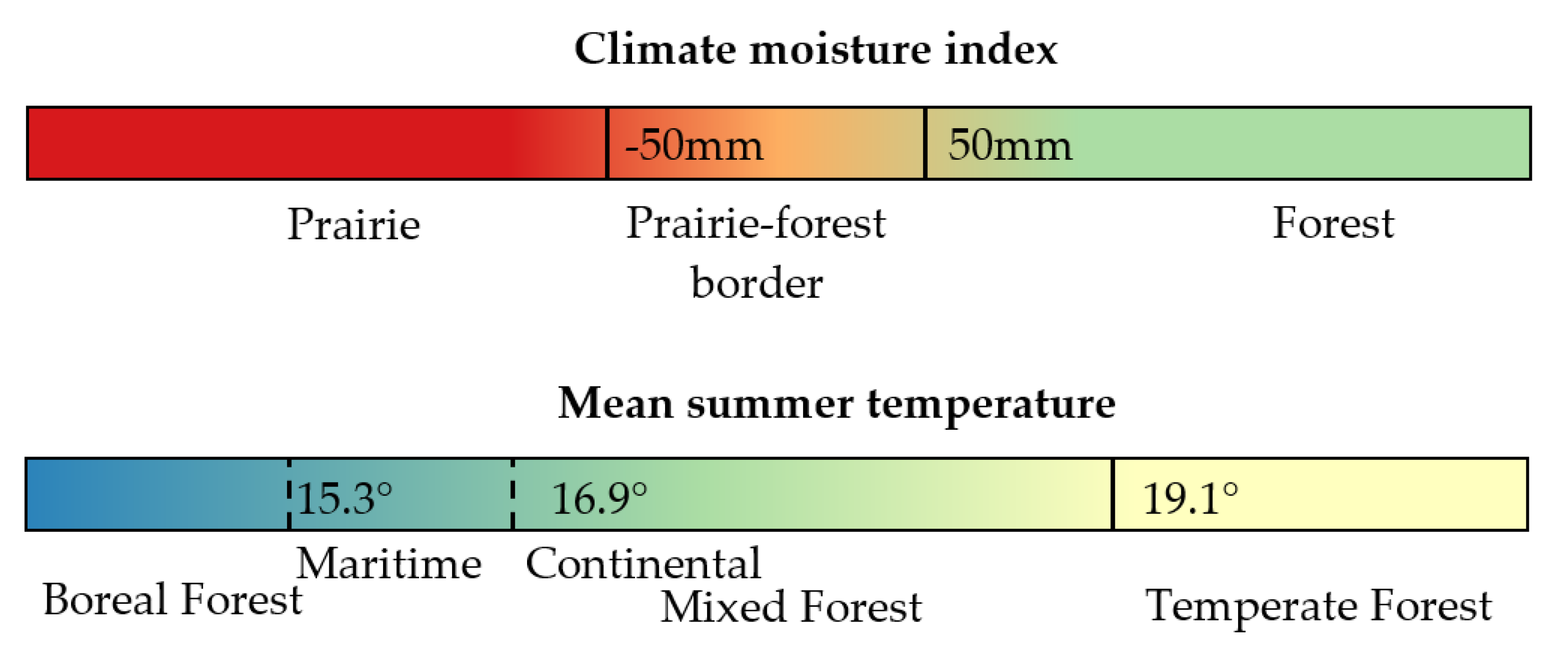
The prairie–forest border ecotone was defined here by a CMI between −50 mm and +50 mm, spanning 100 mm, as shown in Figure 2, corresponding to the approximate range indicated by Danz, Frelich, Reich, and Niemi [14].

Fisichelli, Frelich, and Reich [25] found in Minnesota that the growth of boreal seedlings was surpassed by that of temperate broadleaf saplings (when controlling for browse pressure by white-tailed deer) above 18.1 °C mean summer (June, July, August, or JJA) temperature, defining a threshold between boreal and temperate forest where the composition of forest would be approximately 50:50 boreal and temperate due to equal growth rates of saplings from the two biomes. The range of mean summer temperatures that support the mixed forest would extend to colder and warmer bounds about this mean, representing the edge of nearly pure boreal forest and nearly pure temperate forests, respectively.

The temperature thresholds of the mixed forest climate-biome envelope represented in the model for this study were refined from Fisichelli et al. [25] and Fisichelli et al. [11], who found that currently existing mixed-boreal forest ranged from 16.2–19.1 °C in Minnesota and from 15.8–19.4 °C in Minnesota, Wisconsin and Upper Michigan.

The temperate—mixed forest border was defined by an upper mean summer temperature threshold of 19.1 °C (Figure 2), which was found through a grid search of the threshold in 0.1 degree increments to obtain the best match to the southern range limits of white spruce. White spruce, as opposed to black spruce and tamarack (Larix laracina (Du Roi) K. Koch), primarily grows on upland sites where cold air pooling does not occur [26,27], and is, therefore, a good proxy for the southern bound of the mixed forest.

Here we assumed that the lower mean summer temperature threshold of the mixed forest—the mixed-boreal forest boundary—was partially correlated with the Great Lakes effect on climate. This is indicated by the different summer temperature thresholds in which temperate species could compete with boreal species, as found by Fisichelli et al. [11,25]. Continentality index (CI) is a measure of how much influence large bodies of water have on climate and can be calculated for this region using simple climate and geographic inputs independent of distance to water body:

$$CI=\frac{1.7\ast R}{\sin \left(y+10\right)-14}$$

(6)

where $R$ is the annual range of mean monthly temperatures and $y$ is latitude in degrees [28,29]. That continentality plays a role in the mixed-boreal forest boundary makes physiological sense because maritime areas are associated with milder winters. An approximate extreme minimum temperature threshold for survival of many temperate tree species is between −40 and −45 °C [30], and unlike continental areas, winters near the Great Lakes do not reach those values that are damaging to temperate trees, and consequently, they are able to compete better at lower mean summer temperatures.

Preliminary trials using these thresholds mapped large areas in northern Michigan that are currently mixed forest as boreal. We found by overlaying CI contours on these maps that the areas anomalously mapped as boreal occurred in areas with CI less than approximately 45. We developed a logistic function of CI, that smooths the transition between the relatively warmer and cooler lower mean summer temperature thresholds ($T_{bm}$) that determine the boreal-mixed forest boundary in continental and maritime climates, respectively (Equation (7)):

$$T_{bm}=15.3+\frac{\left(16.9-15.3\right)}{\left(1+\frac{1}{\exp \left(k\ast CI-45\right)}\right)}$$

(7)

where the smoothed transition between the continental and maritime thresholds is centered on CI of 45, with a steepness parameter ($k$) of 0.5, and the temperature constants of 16.9 °C in continental climates and 15.3 °C in maritime climates were found by assessing the model results after 0.1 degree adjustments, and observing that resulting projected maps did not contain anomalous patches of boreal forest in maritime areas. The resulting thresholds are similar to the respective continental climate plots that Fisichelli [25] used in Minnesota and that of the region [11], which included more maritime plots. The range established and used here is slightly broader, probably in part due to the higher resolution of the analysis.

A previously published model used absolute minimum temperatures to define the southern boundary of boreal forest [31], and other work has indicated that a minimum winter temperature threshold defines the limits of the interior boreal forest from coastal hemlock-spruce forest in Alaska [32]. A model tried here used both winter minimum monthly temperature and mean summer temperature to define boreal forest, but resulted in an anomalous boreal patch in northwestern Wisconsin that is currently, and has historically been occupied by mixed forest, rather than boreal forest [33,34,35]. Therefore, the temperature bound in Equation (7) adjusted for continentality was used. Thresholds resulting from these analyses for the prairie–forest border (based on climatic moisture index) and boreal-temperate forest (based on mean summer temperature adjusted for continentality) are shown in Figure 2.

The model to project current and future biome distribution onto maps was built and displayed using R statistical software version 3.4.0 with the RStudio graphical user interface, and the raster, rgdal, dplyr, caret, and rastervis packages [36,37,38,39,40,41]. Resources from the University of Minnesota’s Minnesota Supercomputing Institute (MSI) were used to run the model.

2.3. Climate Data

The CHELSA climate data product at 30 arc-second (roughly 1 km² depending on projection and latitude) resolution [12] was used here. This statistically downscaled climate information is available as a recent 1979–2013 normal (current) and from global circulation models for the years 2061–2080 (2070, future) in multiple representative concentration pathways (RCP) emissions scenarios.

We assessed the current CHELSA climatology monthly mean temperatures against U.S. NOAA and Canadian Weather Service normals for a similar time period (1981–2010) [42,43]. A spatial correlation of differences between these two data sets was apparent in maritime climates near the Great Lakes, especially for the critical summer season, so we compared the difference to CI, calculated from the same CHELSA climatology, for each season as shown in Figure 3. Meteorological seasons are used: winter is December through February (DJF); spring: March through May (MAM), and autumn: September through November (SON).

Linear models were constructed for DJF and SON using linear regression and exponential models for MAM and JJA using non-linear least squares (Appendix A,

Table A1. CHELSA temperature correction model coefficients and error by season.

				Residual Standard Error
	$a$	$b$	$n$
DJF (Equation (A1))	0.0150	-	−1.60	0.675
MAM (Equation (A2))	0.0234	159	−0.959	0.608
JJA (Equation (A2))	0.00437	228	−0.952	0.633
SON (Equation (A1))	0.00816	-	−0.874	0.545

). The models were evaluated using residual plots and lack of fit analysis of variance (ANOVA) (Appendix A). The models were used to adjust the CHELSA monthly maximum and minimum temperatures to more closely reflect the weather station normals.

All terms for the models were significant at p < 0.001 with the exception of the $a$ parameter in both exponential models (Appendix A, Table A1.). This parameter was, however, found to significantly improve the model based on residuals, an ANOVA comparing both a reduced model without the term and a full model with the term, and by the Akaike information criterion, and was therefore kept in both exponential models.

The adjusted recent climate information was used to create a climate-biome envelope model with the definitions described previously (Figure 2.), calculating CI from the adjusted CHELSA normals. The same temperature corrections were applied to the spatially corresponding grid cells for future climate information. CI used for the mixed forest/boreal forest threshold was calculated after the temperature correction described here was performed.

2.4. Global Climate Models and Emissions Scenarios

Because no single model best represents future conditions [44], and because we do not attempt to predict anthropogenic actions with respect to carbon emissions, the climate-biome envelope model was applied to three global climate models that participated in the climate model intercomparison project 5 (CMIP5), and three representative concentration pathway (RCP) scenarios for the years 2041–2060 averaging to 2050, and 2061–2080, averaging to year 2070, to present a range of potential future scenarios. For brevity, only the 2070 analysis is presented here.

Three models were selected to present a range of possible future conditions. In eastern North America, the Beijing Climate Center Climate System Model, version 1.1 (BCC CSM 1.1) [45] runs relatively cold and wet [46]. The Community Climate System Model, version 4 (CCSM4) [47] runs similar to the CMIP5 mean, and the Model for Interdisciplinary Research on Climate, Earth Systems Model (MIROC-ESM) [48] runs relatively hot and dry [44,46].

The scenario RCP 2.6 was run but not included here because it assumes that greenhouse gas emissions peak between 2010 and 2020, and which is almost certainly not the case. Included here are RCP 4.5, which assumes GHG emissions peak around 2040, and decline thereafter; and RCP 8.5, which assumes GHG emissions continue to increase throughout the century [49]. Therefore, six scenarios are presented here; three GCMs by two RCPs for 2070.

2.5. Model Evaluation

The extent of boreal forest in North America has been represented in multiple ways in published literature [34]. Brandt [34] presents one such version against which comparisons could be made, but ultimately, classification is largely dependent on the purpose of the definition [50], and a representation is valuable if it is useful for a given purpose. The classification used here utilizes empirical relationships between vegetation and climate found by scientific study in addition to discoveries made in the course of this study. The classification is useful in that it corresponds to findings of local studies of vegetation, geographic limits of important boreal and temperate species—white spruce and sugar maple—and other modeling efforts and serves the goal of investigating potential vegetation change this century as climate changes.

The prairie forest border presents an additional challenge for quantifiable comparison because of the extent of agricultural development along it. As a result of this and the extent of the prior literature upon which the definition of that ecotone was based, an evaluation of its boundaries is not presented.

The value and emphasis of this study is not the numeric value of the climatic thresholds, but their reasonably accurate representation of vegetation, and most importantly, the utilization addressing potential vegetation change in the region this century.

2.6. Protected Area and Climate-Biome Turnover Analysis

To analyze the difference between future and current climate-biome envelopes, two quantitative analyses were performed. In the first, the land area of each climate-biome was calculated from projected climate-biome envelope model grids by multiplying the number of grid cells in each climate-biome envelope by their resolution. The grids, which are based on the 1983 North American Datum and the GRS80 ellipse with Alber’s Equal Area projection, have a resolution of 648 × 924 m. We then compared the areas of the biomes and ecotones between the two time periods, three GCMs, and two emissions scenarios.

Whereas the first analysis reflects step-size change, for instance, boreal forest to mixed forest, the climate-biome turnover analysis (turnover analysis hereafter) controls for ecotonal gradients, eliminating changes that do not result in an entire biome “turnover”. Turnover of boreal forest is defined as grid cells classified as boreal forest in the recent climate normal and as temperate forest, prairie–forest border, or prairie in 2061–2080. Turnover for mixed and temperate forest is defined as grid cells classified as mixed or temperate forest in the recent climate normal and classified as prairie in 2061–2080. Boreal species loss is defined as the grid cells classified as boreal or mixed forest (both of which can support boreal species) in the recent climate normal and classified as temperate forest, prairie–forest border, or prairie (none of which can support boreal species) in 2061–2080. For this analysis, a confusion matrix, or cross-tabulation, of recent normal climate-biome envelope model values and future model values was created. The percentage of boreal, mixed, and temperate forest grid cells that were classified in the 2070 modeled future scenario as a biome different from the modeled recent normal scenario as defined was then calculated.

The two analyses were performed both for protected areas and over the entire modeled region. Land covered by significant lakes was removed from consideration using spatial data from the Commission for Environmental Cooperation [51].

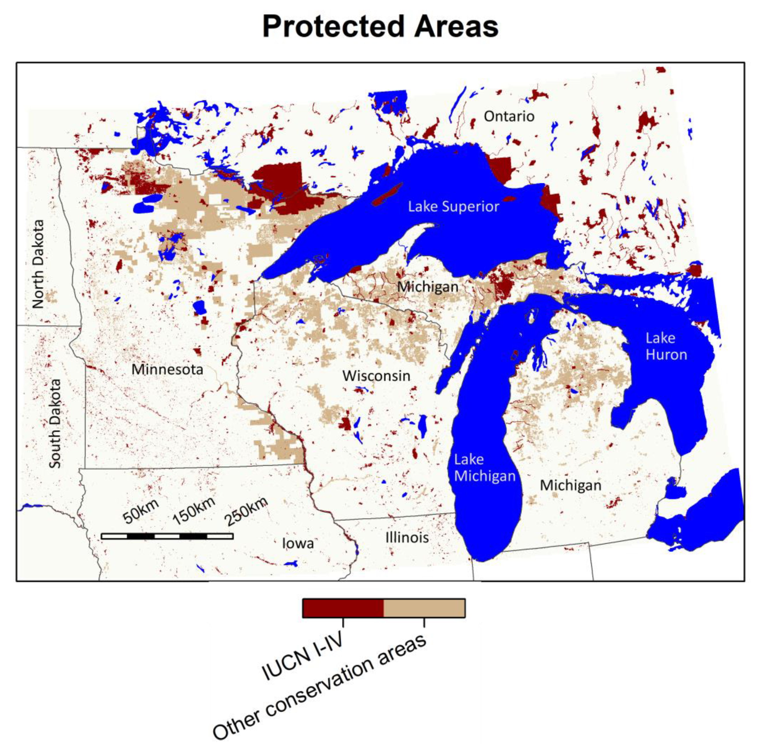
US Geological Survey Gap Analysis Project Protected Areas Data (PAD) [52] and the Canadian Conservation Reporting and Tracking System (CARTS) [53] were utilized to define and outline International Union for the Conservation of Nature (IUCN) classified protected areas in the study area. The analysis presented here includes IUCN categories I–V, lands managed for conservation and recreation, to provide a conservative analysis of protected areas. The analyses were also performed on a second tier of protected areas which includes IUCN categories I–VI, ranging from areas managed for wilderness protection to areas managed for sustainable use of natural resources, and in the PAD database, “other conservation areas” not classified by IUCN, but managed for multiple uses including both resource extraction and conservation (PAD classes I–III). This includes the public forest land in northern Minnesota, Wisconsin, and Michigan, which is managed for multiple uses including conservation, timber, recreation, and mining. For brevity, the analyses of the total land area and the second protected area tier area are presented in Appendix B,

Table A2. Climate-biome envelope total regional areas using a recent normal period, three global climate models and two relative concentration pathway scenarios.

	Global Climate Model	Total Area (km2)
		1979–2013	2061–2080
			RCP 4.5	RCP 8.5
Boreal forest	BCC CSM 1.1	175,782	6764	1
	CCSM4		7512	0
	MIROC ESM		23	0
Mixed forest	BCC CSM 1.1	242,007	211,094	63,693
	CCSM4		177,050	33,177
	MIROC ESM		92,583	14,523
Temperate forest	BCC CSM 1.1	424,955	560,482	580,543
	CCSM4		480,316	491,128
	MIROC ESM		526,284	359,199
Prairie–forest border	BCC CSM 1.1	51,943	47,915	85,590
	CCSM4		86,735	124,203
	MIROC ESM		94,302	88,643
Prairie	BCC CSM 1.1	46,010	114,443	210,870
	CCSM4		189,085	292,189
	MIROC ESM		227,505	478,332

,

Table A3. Climate-biome envelope areas in IUCN I-VI and PAD I-III protected areas, using a recent normal period, three global climate models and two relative concentration pathway scenarios.

		Area (km2)
	Global Climate Model	1979–2013	2061–2080
			RCP 4.5	RCP 8.5
Boreal Forest	BCC CSM 1.1	24,633	1624	0
	CCSM4		1057	0
	MIROC ESM		0	0
Mixed Forest	BCC CSM 1.1	83,207	40,947	9991
	CCSM4		26,485	6000
	MIROC ESM		12,195	3120
Temperate Forest	BCC CSM 1.1	25,424	85,853	102,934
	CCSM4		89,555	92,217
	MIROC ESM		97,498	69,170
Prairie–forest border	BCC CSM 1.1	1574	3568	9775
	CCSM4		9513	16,087
	MIROC ESM		11,171	12,884
Prairie	BCC CSM 1.1	1195	722	2580
	CCSM4		1798	4259
	MIROC ESM		2947	10,085

and

Table A4. Turnover of climate-biome envelopes in total and second tier of protected areas (IUCN classified 1-VI and PAD I-III) protected areas for 1979–2013 and 2061–2080. Turnover of boreal forest is defined as grid cells classified as boreal forest in the recent climate normal classified as temperate forest, prairie–forest border, or prairie in 2061–2080. Turnover for mixed and temperate forest is defined as grid cells classified as mixed or temperate forest in the recent normal and classified as prairie in 2061–2080. Boreal species loss is defined as the grid cells classified as boreal or mixed forest in the recent climate normal and classified as temperate forest, prairie–forest border, or prairie in 2061–2080.

		Turnover (%)
	Global Climate Model	Total Area		IUCN I–VI & PAD I–III
		RCP 4.5	RCP 8.5	RCP 4.5	RCP 8.5
Boreal forest	BCC CSM 1.1	0	64	0	59
	CCSM4	6	81	13	76
	MIROC ESM	47	92	51	87
Mixed forest	BCC CSM 1.1	1	14	0	7
	CCSM4	9	20	3	12
	MIROC ESM	14	42	7	37
Boreal species loss	BCC CSM 1.1	48	85	61	91
	CCSM4	56	92	74	94
	MIROC ESM	78	97	89	97
Temperate forest	BCC CSM 1.1	4	19	3	17
	CCSM4	16	34	15	34
	MIROC ESM	23	65	23	67

. The outlines of both protected area tiers are shown in Figure 4.

3. Results

3.1. Climate-Biome Envelope Model

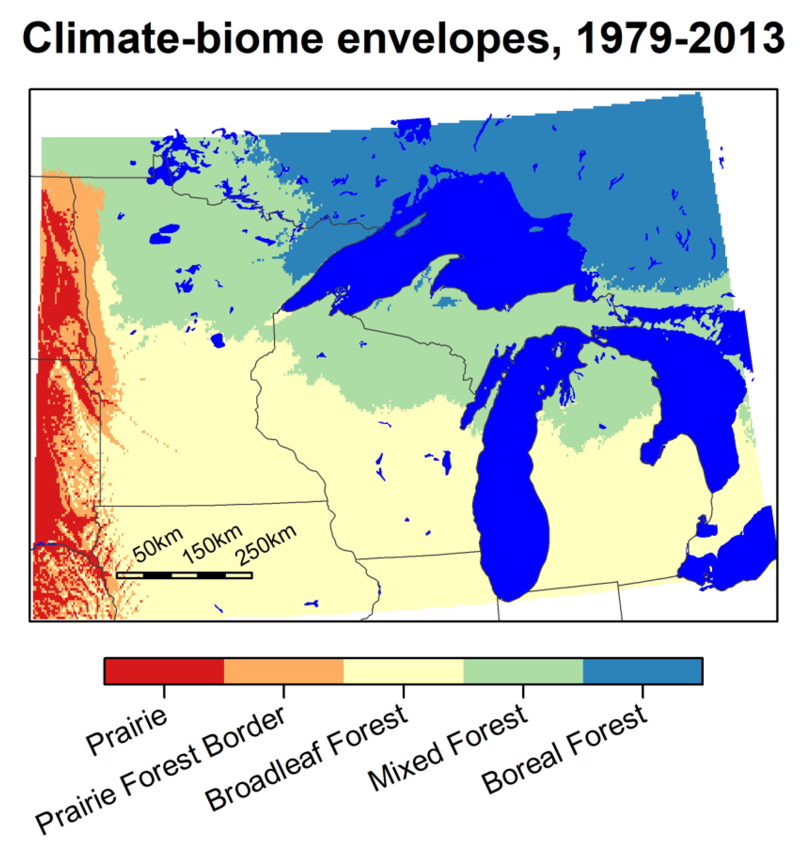
The boreal forest climate-biome envelope for the 1979–2013 period encompasses an area north and east of Lake Superior, as shown in Figure 5. It includes far northeastern Minnesota where land surfaces have slightly higher elevation or are near Lake Superior, and a few small patches of the highlands in upper Michigan. The adjacent mixed forest climate-biome envelope reaches from the boreal forest, south into central Minnesota, Wisconsin, and Lower Michigan. The temperate forest climate-biome envelope covers the remaining southern two-thirds of Lower Michigan, Wisconsin, and Minnesota and areas to the south of that within the spatial domain of our study. The prairie–forest border climatic envelope runs north-south along the western border of Minnesota, adjacent to the mixed forest envelope in the far north, and temperate forest envelope south of that. The prairie climate-biome envelope exists primarily west of the Minnesota—North/South Dakota border, and in far western IA and Nebraska.

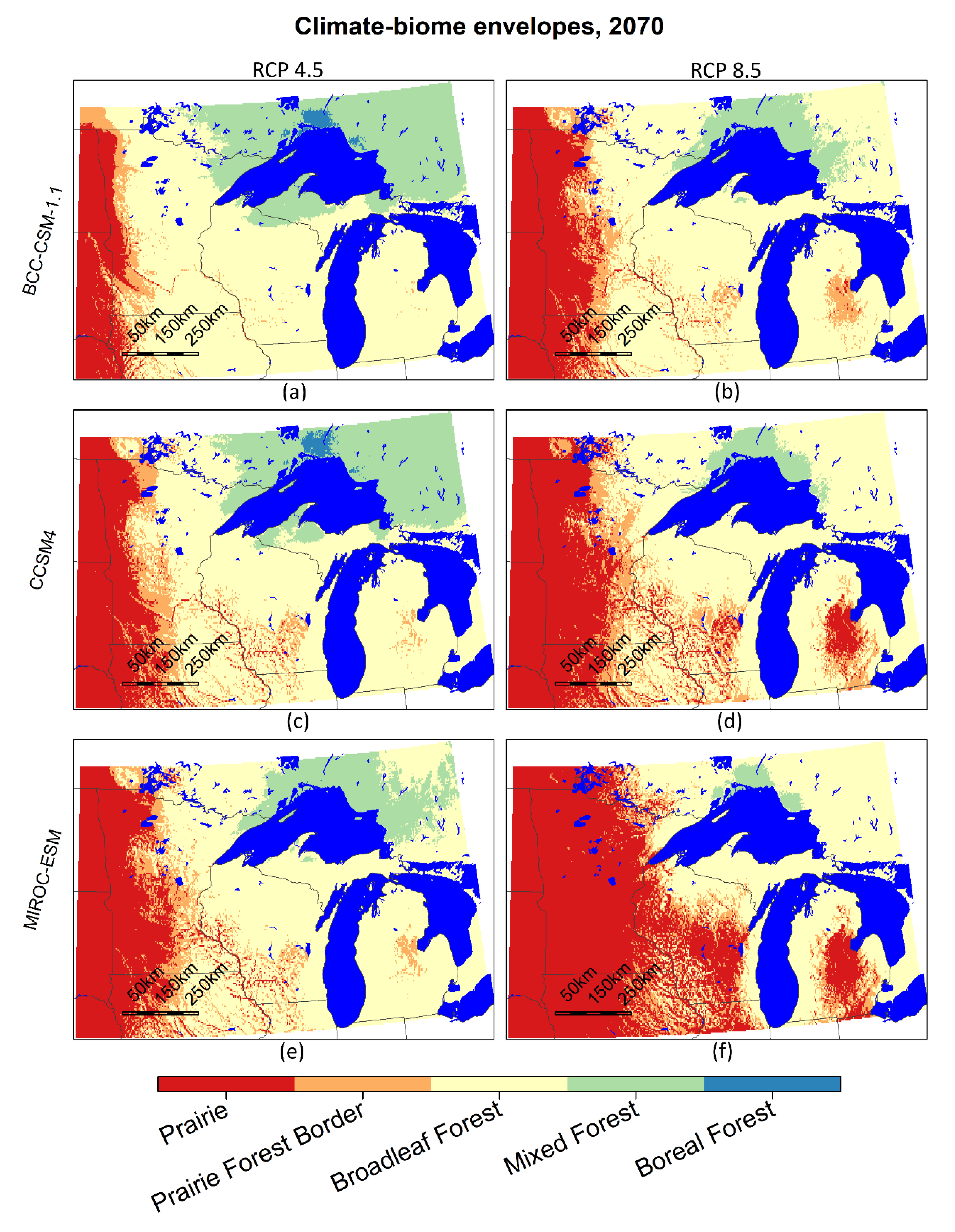
The 2070 projections of the climate-biome envelopes in Figure 6. show an eastward shift of the prairie and prairie forest border climate envelopes, and a decrease in the spatial extent of the mixed and boreal forest climate envelopes in all modeled scenarios. Among models, the magnitude of the changes can be arranged from lowest to highest: BCC-CMS 1.1, CCSM4, MIROC-ESM within each emissions scenario, and the RCP 4.5 scenarios had lower magnitudes of change than the RCP 8.5 scenarios for each model. BCC-CSM 1.1 at RCP 8.5 (6b) indicates a similar shift to that of MIROC-ESM at RCP 4.5 (Figure 6e).

Figure 6a,f had the least and most change among scenarios, respectively, bracketing the future climate conditions investigated here. The cooler, wetter scenario, (Figure 6a) shows a small extent of boreal forest climate envelope remaining north of Lake Superior in 2070; even in this least-change scenario, the extent of land suitable for boreal forest is greatly diminished from its current extent. The mixed forest climate-biome envelope surrounds the boreal climate-biome envelope patch in Ontario, extends west and south into northeastern Minnesota in roughly the same area that boreal forest climate-biome envelope occupies in 1979–2013, and includes approximately two-thirds of upper Michigan. The temperate forest climate-biome envelope occupies a majority of Minnesota, Wisconsin, and Lower Michigan. This envelope covers slightly less than its westerly extent in 1979–2013, but stretches significantly eastward and northward. Prairie and prairie–forest border climate-biome envelopes occupy approximately the western quarter of Minnesota, covering about 50% more than its previous extent.

In the hottest, driest scenario (Figure 6f), the boreal forest climate-biome envelope is eliminated. The mixed forest climate-biome envelope is on the north side of Lake Superior, similar in size and shape to the boreal patch in the cold and wet scenario. The temperate forest climate-biome envelope is smaller than its 1979–2013 extent, or those represented in the other scenarios. It encompasses the mixed forest climate-biome envelope patch in Ontario and extends west into northeastern Minnesota, and covers upper Michigan and northwestern Wisconsin, and encircles Lakes Michigan and Huron in southern Wisconsin and Michigan. The extent of prairie climate-biome envelope is much bigger than the 1979–2013 baseline period and covers approximately 80% of Minnesota and more than half of Wisconsin. The unglaciated regions with rugged topography in southeastern Minnesota and southwestern Wisconsin show a mosaic of prairie, prairie–forest border, and temperate forest climate-biome envelopes surrounded by prairie climate-biome envelope. Prairie climate-biome envelope also covers approximately the center third of Lower Michigan, south and west of Saginaw Bay.

3.2. Protected Area and Climate-Biome Turnover Analyses

Analysis of the boreal forest climate-biome envelope (

Table 1. Comparison of climate-biome envelope areas in protected areas (IUCN classified 1–V) protected areas for 1979–2013 and 2061–2080.

		Area (km2)			% of 1979–2013 Value
	Global Climate Model	1979–2013	2061–2080		2061–2080
			RCP 4.5	RCP 8.5	RCP 4.5	RCP 8.5
Boreal Forest	BCC CSM 1.1	18,692	1353	0	7	0
	CCSM4		971	0	5	0
	MIROC ESM		0	0	0	0
Mixed Forest	BCC CSM 1.1	18,531	21,706	7666	117	41
	CCSM4		16,600	5084	90	27
	MIROC ESM		9555	2688	52	15
Temperate Forest	BCC CSM 1.1	9681	20,734	29,436	214	304
	CCSM4		20,375	27,923	210	288
	MIROC ESM		26,202	23,469	271	242
Prairie–forest border + prairie	BCC CSM 1.1		4886	11,576	275	652
	CCSM4	1775	10,733	15,672	605	883
	MIROC ESM		12,922	22,522	728	1269
Prairie–forest border	BCC CSM 1.1	890	2494	3606	280	405
	CCSM4		4533	4276	509	481
	MIROC ESM		4045	4150	455	466
Prairie	BCC CSM 1.1	885	2391	7971	270	901
	CCSM4		6200	11,397	701	1288
	MIROC ESM		8877	18,372	1003	2076

) indicates a dramatic decrease in extent of climate suitable for boreal forest in protected areas (IUCN I–V) of the region, reaching 0% in every model with the RCP 8.5 scenario as well as MIROC ESM with the RCP 4.5 scenario, and maintaining a maximum of 7% of the current extent in the coldest, wettest scenario (BCC CSM 1.1 with RCP 4.5), from the 1979–2013 recent climate normal period to 2061–2080. Climate suited for mixed forest indicates a wide range of outcomes, from a slight increase in the coldest, wettest scenario (BCC CSM 1.1 with RCP 4.5), to a decrease leaving only 15% of the current spatial extent remaining in protected areas in the hottest and driest scenario (MIROC ESM with RCP 8.5).

Analysis of the protected area within the prairie–forest border and prairie climate-biome envelopes combined (Table 1) shows the spatial extent increasing from 2.7 times in the coldest, wettest scenario (BCC CSM 1.1 with RCP 4.5) to 12.7 times in the hottest, driest scenario (MIROC ESM with RCP 8.5) by 2061–2080 compared to the base period. When including multiple-use public forest land in the US, the spatial extent of protected area in the prairie–forest border climate-biome envelope in 2061–2080 is between 2.5 and 23 times that of 1979–2013 (Appendix B, Table A3).

Analysis of the climate-biome turnover by grid cell in

Table 2. Turnover of climate-biome envelopes in protected areas (IUCN classified 1–V) protected areas for 1979–2013 and 2061–2080. Turnover of boreal forest is defined as grid cells classified as boreal forest in the recent climate normal and as temperate forest, prairie–forest border, or prairie in 2061–2080. Turnover for mixed and temperate forest is defined as grid cells classified as mixed or temperate forest in the recent climate normal and classified as prairie in 2061–2080. Boreal species loss is defined as the grid cells classified as boreal or mixed forest in the recent climate normal and classified as temperate forest, prairie–forest border, or prairie in 2061–2080.

	Global Climate Model	Turnover (%)
		RCP 4.5	RCP 8.5
Boreal forest	BCC CSM 1.1	0	59
	CCSM4	13	73
	MIROC ESM	49	86
Mixed forest	BCC CSM 1.1	1	20
	CCSM4	11	27
	MIROC ESM	21	46
Boreal species loss	BCC CSM 1.1	38	79
	CCSM4	53	86
	MIROC ESM	74	93
Temperate forest	BCC CSM 1.1	5	26
	CCSM4	25	47
	MIROC ESM	34	81

shows that boreal turnover to a combination of temperate forest, prairie forest border, or prairie in protected areas varies widely by GCM and RCP, from 0% in the coldest, wettest scenario (BCC CSM 1.1 with RCP 4.5) to 86% in the hottest, driest scenario (MIROC ESM with RCP 8.5). Boreal species loss in protected areas ranges from 38% to 93%. Mixed forest turnover and temperate forest turnover rates to prairie vary widely based on model and emissions scenario as well, but are as high as 46% and 81% respectively in the hottest, driest scenario. Table A4 shows turnover for the total land area and for the second protected area tier.

4. Discussion

4.1. 1979–2013 Climate-Biome Envelope Model

The location of the boreal-mixed forest border presented in the 1979–2013 model is corroborated by the forest description of the Boundary Waters Canoe Area in Minnesota [1], and on the east side of Lake Superior, it falls very close to the known northern range limits of sugar maple in Lake Superior Provincial Park [54]. It is supported in a recent study by Chaffin [55] who found that temperate species of all size classes decreased dramatically from West to East across the Boundary Waters Canoe Area Wilderness, and were almost entirely absent in the eastern third of the wilderness and adjacent northeastern MN. Finally, the area in northeastern Minnesota mapped as boreal here also corresponds very well to an area previously mapped as subalpine wet forest [33], which is equivalent here to boreal forest.

The mixed forest climate-biome envelope accurately includes Itasca State Park in Minnesota [56], and the southern border of the mixed forest climate-biome envelope follows the southern range of white spruce very closely—mostly within 20 km, but with a narrow 50 km deviation in the St. Croix River valley on the Minnesota-Wisconsin state line.

As expected, the prairie–forest border as shown by the 1979–2013 model is oriented more north-south and further west than familiar prairie–forest border delineations based on pre-European settlement data [15]. It has been shown that the climate, especially near the prairie–forest border in Minnesota, was significantly wetter during 1979–2013 than pre-European settlement, while experiencing little summer warming, resulting in a wetter climate at the end of the twentieth century [15,17], which results in a climate suitable for forests further west than typically delineated. In addition, fire use by Native Americans prior to European settlement allowed some areas of prairie to exist east of the border as defined by climate [3]. Other analyses of biome climate envelopes for the late 20th Century [10,33], also place the prairie–forest border in a north-south orientation right along the western edge of Minnesota, and eastern North Dakota and South Dakota, while Gonzalez et al. [57] places it also in a north-south orientation, but slightly further west.

The rule-based model developed here to map boreal, mixed forest and temperate forest is an improvement over previous efforts to map forest biomes in the region. For example, boreal forest is clearly a better classification for the previously mentioned patch of forest in northeastern Minnesota (Figure 4) that was classified as subalpine forest by Lugo et al. [33], since the elevation of the area does not support the subalpine classification. Boreal conifer forest was shown covering the northern one-fourth of Minnesota by Gonzalez et al. [57], placing the boreal/mixed forest border too far south, including large swaths of forest with high percentages of temperate tree species. Despite improvements made here, limitations related to effects of cold-air pooling and other local topographical effects, and effects of the Great Lakes (other than those we were able to take into account through continentality adjustments) were encountered. The next generation of models should attempt to incorporate topographic effects that we could not account for here, including cold air pooling in lowlands [58], cold water upwelling in deep lakes [59], and north-south slope effects, which could potentially account for inclusions of boreal forest within the temperate biome, and vice versa, at finer spatial scales. Furthermore, the results emphasized here are differences between the current and future climate-biome envelopes, especially with respect to protected areas, and it is likely that the range of uncertainty covered by the multiple GCM’s and emissions scenarios dwarfs uncertainty in the climate-biome envelope definitions. Although the range of possibilities is somewhat broad, it demonstrates that more extreme shifts are likely if carbon emissions are not curbed soon and indicates clear trends from which implications can be drawn.

4.2. 2061–2080 Projections, Protected Area and Turnover Analysis

Although timing and specific geography will depend on the multitude of factors that determine existing vegetation, projections reported here for 2061–2080 agree with previous analyses that northeastward shifts in biomes are likely to occur in this region, with loss of conifer forest and replacement of forests by grasslands that vary in magnitude depending on the GCM and carbon emissions scenarios examined [2,60]. The 2061–2080 climate-biome envelope model indicates that the projected climate change in two of the six scenario/model combinations will eliminate areas suitable to boreal forest from the study region. Two more of the modeled scenarios show only a diminutively small spatial extent of boreal forest remaining by 2070. The analysis of climate-biome envelope in protected areas suggests that it will be very difficult to conserve boreal forest in the region in the future. The turnover analysis and the boreal species loss shown here indicate that vegetation, especially boreal species, at many locations will no longer be suited to the climate at those locations. Boreal forest will likely continue to exist further north than this study area, and there is a possibility of boreal forest being retained in small areas with cold air pooling or cold water upwelling not captured by the climate information used here. Local efforts are key to cataloging and retaining potential boreal forest refugia. Resilience management strategies, or improving the ability of ecosystems to return to their un-disturbed state [61], such as maintaining diversity and other strategies like those outlined in Galatowitsch et al. [2] should be used in order to conserve potential boreal refugia where possible and support regional diversity.

The future projections of the climate-biome envelopes corroborate predictions that both the prairie and the temperate forest may establish northeast of their current locations. There may be an opportunity to manage prairie and oak savanna in the northern part of the region. Just as conservation of healthy savanna and prairie is currently made difficult by the paucity of protected lands in the southwestern part of the study region, the concentration and size of protected lands in the northern part of the region may help make large-scale management and conservation of prairie and savanna achievable in the region. An increase in fire severity due to the drier climate and a possible increase in fire frequency in the northern part of the region may hasten and assist transition of forest to fire-dependent prairie and prairie–forest border [3]. It will likely be pertinent to use response management strategies [61] to facilitate ecosystem change with a goal of managing land for oak savanna and prairie in many locations throughout the range where the prairie–forest border and prairie climate-biome envelopes may be in the future. For instance, because of the high velocity of change expected in the region, and as indicated by the high rates of biome turnover shown here, establishing oak savanna or prairie in the protected areas that now harbor mixed and boreal forest, assisted migration will likely be important [2,19,61]. It is important that plant communities, ecotones, and biomes currently in the southern portion of the study area, especially those that have been nearly eliminated such as oak savanna and prairie, remain healthy where they exist, and expand if possible, as they may be important seed sources and ecosystem blueprints for future off-site restoration of prairie and savanna in large protected areas of the north which may have suitable climates. Research on oak savanna and prairie ecosystem dynamics continues to be extremely valuable.

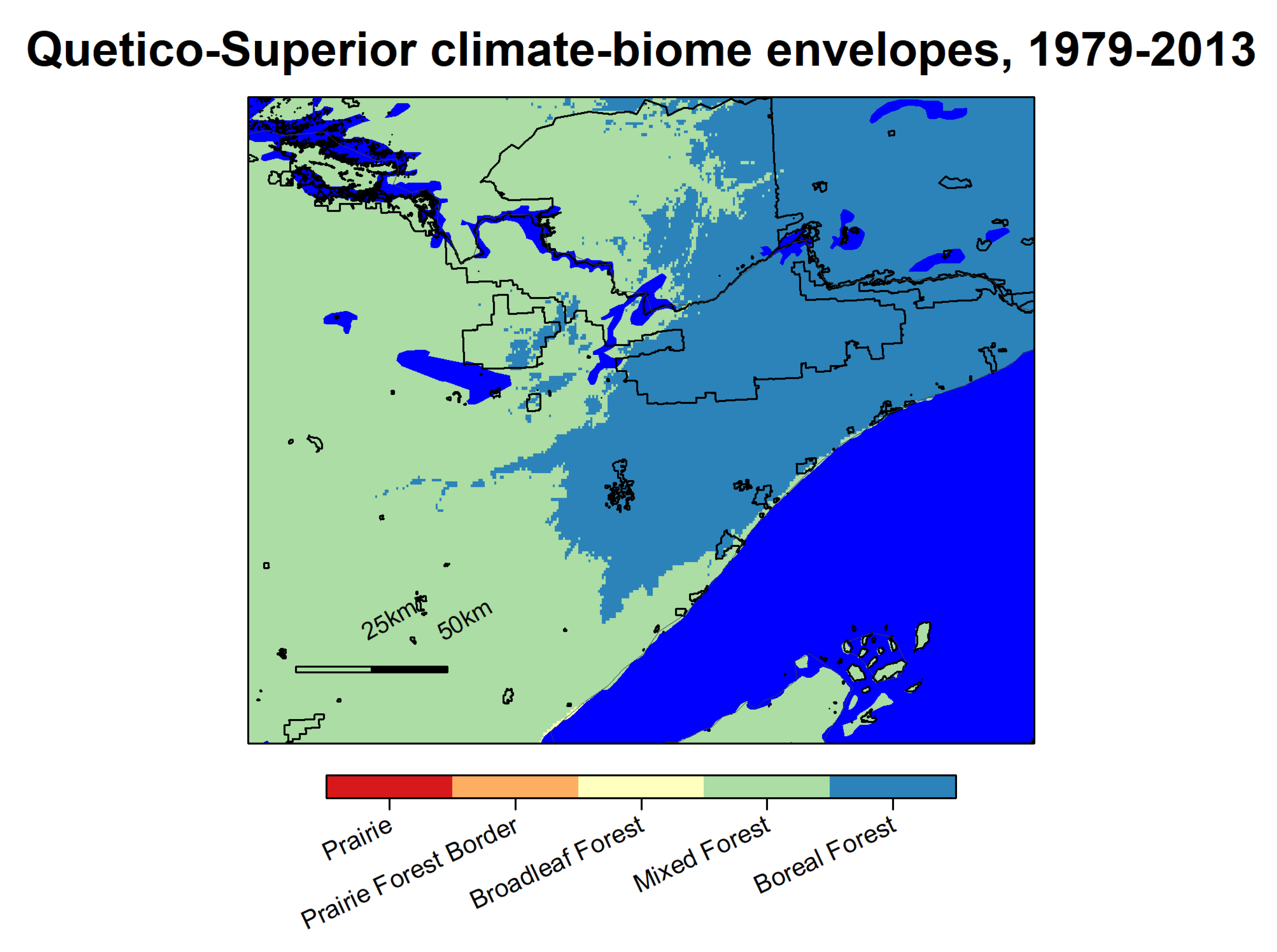
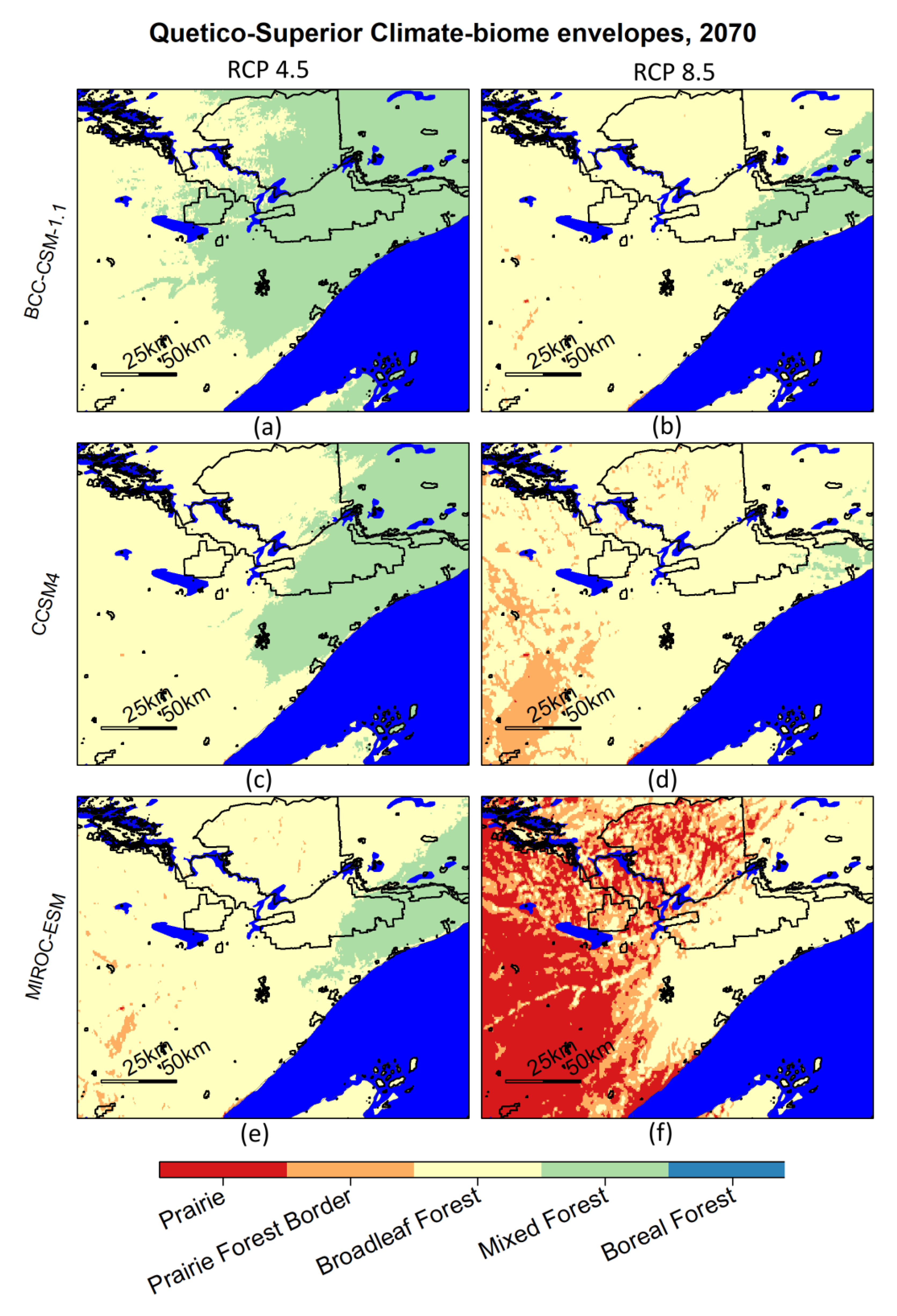
An important example of protected areas at risk of biome change is the QSE, with its nearly one million ha of wilderness and large tracts of unlogged boreal and near-boreal mixed forest that constitute the premiere natural areas within the study region (Figure 7). Our analysis shows that climate in this area may not support mixed and boreal forest by 2070 (Figure 8). Although small boreal refugia may still exist, maintaining these boreal species widely will not be possible via resistance (actively managing to prevent any vegetative change in a changing climate) and resilience strategies [61], and facilitation of conversion to temperate oak and maple forests, oak savannas, or prairies may be needed [62]. The future climate-biome envelope for the region that the QSE currently resides in varies depending on the emissions scenario/GCM combination. In cool and wet scenarios, the area is near the edge of the mixed forest and would likely support some boreal refugia. But in the hot and dry scenario presented here, the climate in this area could support prairie–forest border ecosystems by 2070 (Figure 8).

This analysis indicates that, in general, some conservation opportunities will close and some will arise due to a changing climate and the heterogeneous spatial arrangement of protected lands. Landscape wide, conservation efforts will, of necessity, balance between maintaining healthy ecosystems in the present, which may include managing for resistance or resilience, and facilitating change to accommodate future climates. In this way, as climate change presents great problems for diverse and stable ecosystems, and potentially novel opportunities to manage for or conserve diverse ecosystems in biomes and ecotones landscape-scale diversity may be maximized for the given conditions.

5. Conclusions

The climate-biome envelope model presented here shows good correspondence with other modeling efforts and provides valuable insight for the study region. The projections for the years 2061–2080 show that the region will likely lose most of its suitable climate for boreal forest and thus lose most of its boreal forest eventually, perhaps retaining some small portion north of Lake Superior. In the hottest and driest scenario, the US portion of the study area and the landscapes of the Boundary Waters Canoe Area Wilderness and Quetico Provincial Park in the current QSE, lose all mixed forest climate-biome envelope, indicating the loss of a climatic niche for boreal species entirely. These scenarios indicate that, unless a low greenhouse gas emissions scenario is achieved by society soon, the prairie–forest border is likely to move northeast and fall within larger swaths of protected areas in Northeastern Minnesota and Northern Wisconsin. Therefore, under a business as usual climate change scenario (i.e., RCP 8.5) these lands represent potential opportunities for prairie and savanna replenishment—extremely diverse ecosystems that have been nearly lost due to land transformation—at large spatial extents not seen since European settlement. This opportunity arises due to the unique juxtaposition of three biomes on the current landscape, the heterogeneous pattern of human development in the region and the location of protected lands. It illustrates that climate change poses many problems for conservation and biodiversity, but may also present novel opportunities to manage for ecosystems that are currently difficult to conserve.

References

- Heinselman, M.L. Boundary Waters Wilderness Ecosystem; University of Minnesota Press: Minneapolis, MN, USA; London, UK, 1996; ISBN 0816628041. [Google Scholar]
- Galatowitsch, S.; Frelich, L.E.; Phillips-Mao, L. Regional climate change adaptation strategies for biodiversity conservation in a midcontinental region of North America. Boil. Conserv. 2009, 142, 2012–2022. [Google Scholar] [CrossRef]
- Frelich, L.E.; Reich, P.B. Will environmental changes reinforce the impact of global warming on the prairie– forest border of central North America? Front. Ecol. Environ. 2010, 8, 371–378. [Google Scholar] [CrossRef]
- Reich, P.B.; Sendall, K.M.; Rice, K.; Rich, R.; Stefanski, A.; Hobbie, S.; Montgomery, R.A. Geographic range predicts photosynthetic and growth response to warming in co-occurring tree species. Nat. Clim. Chang. 2015, 5, 148–152. [Google Scholar] [CrossRef]
- Reich, P.B.; Sendall, K.M.; Stefanski, A.; Rich, R.L.; Hobbie, S.; Montgomery, R.A. Effects of climate warming on photosynthesis in boreal tree species depend on soil moisture. Nature 2018, 562, 263–267. [Google Scholar] [CrossRef]
- Nuzzo, V.A. Extent and status of Midwest oak savanna: Presettlement and 1985. Nat. Areas J. 1986, 6, 6–36. [Google Scholar]
- Samson, F.; Knopf, F. Prairie Conservation in North America. Bioscience 1994, 44, 418–421. [Google Scholar] [CrossRef] [Green Version]
- OpenStreetMap Contributors Planet Dump. Available online: https://planet.osm.org (accessed on 13 September 2020).
- McNab, H.; Cleland, D.; Freeouf, J.; Keys, J.; Nowacki, G.; Carpenter, C. Description of ecological subregions: Sections of the conterminous United States. Gen. Tech. Rep. WO-76B 2007, 76, 1–82. [Google Scholar]
- Prentice, I.C.; Cramer, W.; Harrison, S.P.; Leemans, R.; Monserud, R.A.; Solomon, A.M. Special Paper: A Global Biome Model Based on Plant Physiology and Dominance, Soil Properties and Climate. J. Biogeogr. 1992, 19, 117. [Google Scholar] [CrossRef]
- Fisichelli, N.; Frelich, L.E.; Reich, P.B. Temperate tree expansion into adjacent boreal forest patches facilitated by warmer temperatures. Ecography 2013, 37, 152–161. [Google Scholar] [CrossRef]
- Karger, D.N.; Conrad, O.; Böhner, J.; Kawohl, T.; Kreft, H.; Soria-Auza, R.W.; Zimmermann, N.E.; Linder, H.P.; Kessler, M. Climatologies at high resolution for the earth’s land surface areas. Sci. Data 2017, 4, 170122. [Google Scholar] [CrossRef] [Green Version]
- Hogg, E. (Ted) Temporal scaling of moisture and the forest-grassland boundary in western Canada. Agric. For. Meteorol. 1997, 84, 115–122. [Google Scholar] [CrossRef] [Green Version]
- Danz, N.P.; Frelich, L.E.; Reich, P.B.; Niemi, G.J. Do vegetation boundaries display smooth or abrupt spatial transitions along environmental gradients? Evidence from the prairie–forest biome boundary of historic M innesota, USA. J. Veg. Sci. 2013, 24, 1129–1140. [Google Scholar] [CrossRef]
- Danz, N.P.; Reich, P.B.; Frelich, L.E.; Niemi, G. Vegetation controls vary across space and spatial scale in a historic grassland-forest biome boundary. Ecography 2010, 34, 402–414. [Google Scholar] [CrossRef]
- Williams, J.W.; Shuman, B.N.; Webb, T.; Bartlein, P.J.; Leduc, P.L. Late-Quaternay vegetation dynamics in North America: Scaling from taxa to biomes. Ecol. Monogr. 2004, 74, 309–334. [Google Scholar] [CrossRef] [Green Version]
- Millett, B.; Johnson, W.C.; Guntenspergen, G. Climate trends of the North American prairie pothole region 1906–2000. Clim. Chang. 2009, 93, 243–267. [Google Scholar] [CrossRef]
- Bennett, S.; Wernberg, T.; Joy, B.A.; De Bettignies, T.; Campbell, A. Central and rear-edge populations can be equally vulnerable to warming. Nat. Commun. 2015, 6, 10280. [Google Scholar] [CrossRef]
- Batllori, E.; Parisien, M.-A.; Parks, S.A.; Moritz, M.A.; Miller, C. Potential relocation of climatic environments suggests high rates of climate displacement within the North American protection network. Glob. Chang. Boil. 2017, 23, 3219–3230. [Google Scholar] [CrossRef]
- Hannah, L.; Midgley, G.F.; Millar, D. Climate change-integrated conservation strategies. Glob. Ecol. Biogeogr. 2002, 11, 485–495. [Google Scholar] [CrossRef] [Green Version]
- Prasad, A.M.; Iverson, L.R.; Matthews, S.; Peters, M. A Climate Change Atlas for 134 Forest Tree Species of the Eastern United States. Available online: https://www.nrs.fs.fed.us/atlas/tree (accessed on 9 January 2019).
- Hällfors, M.H.; Aikio, S.; Fronzek, S.; Hellmann, J.; Ryttäri, T.; Heikkinen, R. Assessing the need and potential of assisted migration using species distribution models. Boil. Conserv. 2016, 196, 60–68. [Google Scholar] [CrossRef] [Green Version]
- Hogg, E. (Ted) Climate and the southern limit of the western Canadian boreal forest. Can. J. For. Res. 1994, 24, 1835–1845. [Google Scholar] [CrossRef]
- Lowe, P.R. An Approximating Polynomial for the Computation of Saturation Vapor Pressure. J. Appl. Meteorol. 1977, 16, 100–103. [Google Scholar] [CrossRef] [Green Version]
- Fisichelli, N.; Frelich, L.E.; Reich, P.B. Sapling growth responses to warmer temperatures ‘cooled’ by browse pressure. Glob. Chang. Boil. 2012, 18, 3455–3463. [Google Scholar] [CrossRef]
- Wolken, J.M.; Landhausser, S.M.; Lieffers, V.J.; Silins, U. Seedling growth and water use of boreal conifers across different temperatures and near-flooded soil conditions. Can. J. For. Res. 2011, 41, 2292–2300. [Google Scholar] [CrossRef]
- Society of American Foresters. Forest Cover Types of the Eastern United States; Report of the Committee on Forest Types, Society of American Foresters; Society of American foresters: Washington, DC, USA, 1940. [Google Scholar]
- Kopec, R.J. Continentality around the Great Lakes. Bull. Am. Meteorol. Soc. 1965, 46, 54–57. [Google Scholar] [CrossRef] [Green Version]
- Conrad, V. Usual formulas of continentality and thiir limits of validity. Trans. Am. Geophys. Union 1948, 27, 663–664. [Google Scholar] [CrossRef]
- Sakai, A.; Weiser, C.J. Freezing Resistance of Trees in North America with Reference to Tree Regions. Ecology 1973, 54, 118–126. [Google Scholar] [CrossRef]
- Lenihan, J.M.; Neilson, R.P. A Rule-Based Vegetation Formation Model for Canada. J. Biogeogr. 1993, 20, 615. [Google Scholar] [CrossRef]
- Hopkins, D.M. Some Characteristics of the Climate in Forest and Tundra Regions in Alaska. Arctic 1959, 12, 214–220. [Google Scholar] [CrossRef]
- Lugo, A.E.; Brown, S.L.; Dodson, R.; Smith, T.S.; Shugart, H.H. The Holdridge life zones of the conterminous United States in relation to ecosystem mapping. J. Biogeogr. 1999, 26, 1025–1038. [Google Scholar] [CrossRef]
- Brandt, J. The extent of the North American boreal zone. Environ. Rev. 2009, 17, 101–161. [Google Scholar] [CrossRef]
- Stearns, F.W. History of the Lake States Forests: Natural and Human Impacts; Gen. Tech. Rep. NC; U.S. Department of Agriculture: St. Paul, MN, USA, 1981.
- R Core Team R: A Language and Environment for Statistical Computing. Available online: http://www.r-project.org/ (accessed on 12 March 2019).
- Hijmans, R.J. Raster: Geographic Data Analysis and Modeling. Available online: https://cran.r-project.org/package=raster (accessed on 30 January 2019).
- Bivand, R.; Keitt, T.; Rowlingson, B. Rgdal: Bindings for the “Geospatial” Data Abstraction Library. Available online: https://cran.r-project.org/package=rgdal (accessed on 15 March 2019).
- Wickham, H.; Francois, R.; Henry, L.; Müller, K. Dplyr: A Grammar of Data Manipulation. Available online: https://cran.r-project.org/package=dplyr (accessed on 15 February 2019).
- Perpiñán, O.; Hijmans, R. RasterVis. Available online: http://oscarperpinan.github.io/rastervis/ (accessed on 17 March 2019).
- Kuhn, M.; From, C.; Wing, J.; Weston, S.; Williams, A.; Keefer, C.; Engelhardt, A.; Cooper, T.; Mayer, Z.; Kenkel, B.; et al. Caret: Classification and Regression Training. Available online: https://cran.r-project.org/package=caret (accessed on 26 March 2019).
- NOAA 1981-2010 US Climate Normals. Available online: https://www.ncdc.noaa.gov/data-access/land-based-station-data/land-based-datasets/climate-normals/1981-2010-normals-data (accessed on 23 July 2018).
- Environment and Climate Change Canada Canadian Climate Normals & Averages 1981–2010. Available online: http://climate.weather.gc.ca/climate_normals/ (accessed on 23 July 2018).
- Sheffield, J.; Barrett, A.P.; Colle, B.; Fernando, D.N.; Fu, R.; Geil, K.; Hu, Q.; Kinter, J.; Kumar, S.; Langenbrunner, B.; et al. North American Climate in CMIP5 Experiments. Part I: Evaluation of Historical Simulations of Continental and Regional Climatology. J. Clim. 2013, 26, 9209–9245. [Google Scholar] [CrossRef] [Green Version]
- Xin, X.; Wu, T.; Zhang, J. Introductions to the CMIP 5 simulations conducted by the BCC climate system model (in Chinese). Adv. Clim. Chang. Res. 2012, 8, 378–382. [Google Scholar]
- Cook, B.I.; Smerdon, J.E.; Seager, R.; Coats, S. Global warming and 21stcentury drying. Clim. Dyn. 2014, 43, 2607–2627. [Google Scholar] [CrossRef] [Green Version]
- Gent, P.R.; Danabasoglu, G.; Donner, L.J.; Holland, M.M.; Hunke, E.C.; Jayne, S.R.; Lawrence, D.; Neale, R.B.; Rasch, P.J.; Vertenstein, M.; et al. The Community Climate System Model Version 4. J. Clim. 2011, 24, 4973–4991. [Google Scholar] [CrossRef]
- Watanabe, M.; Suzuki, T.; O’Ishi, R.; Komuro, Y.; Watanabe, S.; Emori, S.; Takemura, T.; Chikira, M.; Ogura, T.; Sekiguchi, M.; et al. Improved Climate Simulation by MIROC5: Mean States, Variability, and Climate Sensitivity. J. Clim. 2010, 23, 6312–6335. [Google Scholar] [CrossRef]
- Meinshausen, M.; Smith, S.J.; Calvin, K.; Daniel, J.S.; Kainuma, M.L.T.; Lamarque, J.-F.; Matsumoto, K.; Montzka, S.A.; Raper, S.C.B.; Riahi, K.; et al. The RCP greenhouse gas concentrations and their extensions from 1765 to 2300. Clim. Chang. 2011, 109, 213–241. [Google Scholar] [CrossRef] [Green Version]
- Sims, R.A.; Corns, I.G.W.; Klinka, K. Introduction-global to local: Ecological Land Classification. Environ. Monit. Assess. 1996, 39, 1–10. [Google Scholar] [CrossRef]
- Commission for Environmental Cooperation North American Atlas-Hydrography. Available online: http://nationalatlas.gov/atlasftp-na.html (accessed on 12 June 2018).
- Gergely, K.J.; McKerrow, A. PAD-US—National Inventory of Protected Areas (ver. 1.4 Combined Feature Class). Available online: https://gapanalysis.usgs.gov/padus/ (accessed on 6 July 2016).
- Canadian Council on Ecological Areas (CCEA). Conservation Areas Reporting and Tracking System (CARTS). Available online: http://www.ccea.org/carts/ (accessed on 19 January 2018).
- Goldblum, D.; Rigg, L.S.; Goldblum, D.; Rigg, L.S. Age structure and regeneration dynamics of sugar maple at the deciduous/boreal forest ecotone, Ontario, Canada. Phys. Geogr. 2002, 23, 115–129. [Google Scholar] [CrossRef]
- Chaffin, D. Climate Change and Future Forests of the Boundary Waters Canoe Area Wilderness: An assessment of Temperate Tree Abundance, Earthworm Invasion and Understory Regeneration Trends; University of Minnesota: Minneapolis, MN, USA, 2019. [Google Scholar]
- Zenner, E.K.; Peck, J.E. Maintaining a Pine Legacy in Itasca State Park. Nat. Areas J. 2009, 29, 157–166. [Google Scholar] [CrossRef]
- Gonzalez, P.; Neilson, R.P.; Lenihan, J.M.; Drapek, R.J. Global patterns in the vulnerability of ecosystems to vegetation shifts due to climate change. Glob. Ecol. Biogeogr. 2010, 19, 755–768. [Google Scholar] [CrossRef]
- Sartz, R. Effect of Topography on Microclimate in Southwestern Wisconsin; North Central Experimentation Station, Forest Service, US Department of Agriculture: St. Paul, MN, USA, 1972.
- Plattner, S.; Mason, D.M.; Leshkevich, G.A.; Schwab, D.J.; Rutherford, E.S. Classifying and Forecasting Coastal Upwellings in Lake Michigan Using Satellite Derived Temperature Images and Buoy Data. J. Great Lakes Res. 2006, 32, 63–76. [Google Scholar] [CrossRef]
- Bachelet, M.; Neilson, R.P.; Lenihan, J.M.; Drapek, R.J. Climate Change Effects on Vegetation Distribution and Carbon Budget in the United States. Ecosystems 2001, 4, 164–185. [Google Scholar] [CrossRef]
- Millar, C.I.; Stephenson, N.L.; Stephens, S.L. Climate change and forests of the future: Managing in the face of uncertainty. Ecol. Appl. 2007, 17, 2145–2151. [Google Scholar] [CrossRef] [PubMed]
- Frelich, L.E.; Jõgiste, K.; Stanturf, J.; Jansons, A.; Vodde, F. Are Secondary Forests Ready for Climate Change? It Depends on Magnitude of Climate Change, Landscape Diversity and Ecosystem Legacies. Forests 2020, 11, 965. [Google Scholar] [CrossRef]
Figure 1.
The study area extent in North America. Basemap © OpenStreetMap contributors [8].
Figure 2.
Visual summary of climate-biome envelope model definitions.
Figure 3.
CHELSA 1979–2013 and U.S. NOAA 1981–2010 temperature comparisons and correction models.
Figure 4.
Protected areas considered for analysis of protected climate-biome envelope areas. Dark red indicates the conservative estimate of “protected” status addressed in this study, IUCN classification I–V. Tan indicates “other conservation areas” meeting PAD criteria I II or III and IUCN classification VI (analysis included in Appendix B). Alber’s Equal Area projection.
Figure 5.
Climate-biome envelopes in the Lake States region for the years 1979–2013. Alber’s Equal Area projection.
Figure 6.
Climate-biome envelopes for the Lake States region for the years 2061–2080. Tiles represent two emissions scenarios and three CMIP5 global climate models. Alber’s Equal Area projection.
Figure 7.
Quetico-Superior ecosystem biomes for the 1979–2013 period. IUCN categories I–V are outlined in black and include Quetico Provincial Park, the Boundary Waters Canoe Area Wilderness, Voyageurs National Park, and others. Albers Equal Area projection.
Figure 8.
Quetico-Superior ecosystem biomes for the 2061–2080 period. Tiles represent two emissions scenarios and three CMIP5 global climate models. IUCN categories I–V are outlined in black and include Quetico Provincial Park, the Boundary Waters Canoe Area Wilderness, Voyageurs National Park, and others. Albers Equal Area projection.