Applying Multi-Temporal Landsat Satellite Data and Markov-Cellular Automata to Predict Forest Cover Change and Forest Degradation of Sundarban Reserve Forest, Bangladesh

Abstract

Overdependence on and exploitation of forest resources have significantly transformed the natural reserve forest of Sundarban, which shares the largest mangrove territory in the world, into a great degradation status. By observing these, a most pressing concern is how much degradation occurred in the past, and what will be the scenarios in the future if they continue? To confirm the degradation status in the past decades and reveal the future trend, we took Sundarban Reserve Forest (SRF) as an example, and used satellite Earth observation historical Landsat imagery between 1989 and 2019 as existing data and primary data. Moreover, a geographic information system model was considered to estimate land cover (LC) change and spatial health quality of the SRF from 1989 to 2029 based on the large and small tree categories. The maximum likelihood classifier (MLC) technique was employed to classify the historical images with five different LC types, which were further considered for future projection (2029) including trends based on 2019 simulation results from 1989 and 2019 LC maps using the Markov-cellular automata model. The overall accuracy achieved was 82.30%~90.49% with a kappa value of 0.75~0.87. The historical result showed forest degradation in the past (1989–2019) of 4773.02 ha yr⁻¹, considered as great forest degradation (GFD) and showed a declining status when moving with the projection (2019–2029) of 1508.53 ha yr⁻¹ and overall there was a decline of 3956.90 ha yr⁻¹ in the 1989–2029 time period. Moreover, the study also observed that dense forest was gradually degraded (good to bad) but, conversely, light forest was enhanced, which will continue in the future even to 2029 if no effective management is carried out. Therefore, by observing the GFD, through spatial forest health quality and forest degradation mapping and assessment, the study suggests a few policies that require the immediate attention of forest policy-makers to implement them immediately and ensure sustainable development in the SRF.

1. Introduction

Mangrove forests (MFs), are predominantly observed along the inter-tidal coastlines across the world where land meets with the sea [1]. Forty-one percent of the world’s mangroves exist in South and Southeast Asia and the remaining 59% are shared by other regions (East Asia, Pacific Islands, Middle East, North and Central America and the Caribbean, South America, Eastern and Southern Africa, and West and Central Africa) worldwide [2]. Globally, MF plays an important role in countries’ national economies through natural productivity and the variety of its products and services [3]. Moreover, mangroves protect coastal areas from severe cyclonic storms, save valuable human lives and properties, as well as preserve habitats of endangered species [4,5]. However, the Sundarban Reserve Forest (SRF), including MF, is located between Bangladesh and India and is the largest continuous MF patch (approximately 10,300 km² or 1,030,000 ha) and, in Bangladesh, a major portion (about 60%) of it, 6017.22 km² or 601,722 ha, is found, and the rest is in India [6].

The SRF is considered as one of the world’s most endangered tropical ecosystems [7], which has been threatened over the past 30 years by several activities, such as industrialization, extensive crab and shrimp farming, agricultural production, natural disasters such as cyclones and tidal surges [8], climate change [9], unsustainable human activities, etc. [10,11]. These changes have taken place on the Earth’s surface by the significant land surface conversions [12], considered as an important factor for environmental degradation in any landscape [13]. For example, due to cyclones and natural disasters, forests experience additional stress to their biodiversity [14]. In connection with this, sea-level projection data suggest that a rise in sea level from 32–88 cm will lead to the total disappearance of mangroves by 2100 [15,16,17].

However, to date, there are insufficient studies conducted in SRF, especially in the Bangladesh Sundarban part, to monitor its trend changes related to several drivers including its future changes and degradation. Therefore, monitoring, analysis, modeling and transformation of Land Use and Land Cover (LULC) changes are significantly important for conservation, planning and ecosystem management activities [18,19,20], so distribution and dynamics studies must first be completed [21] under the past and present data lens, which will play a key role in the decision-making process [22]. To investigate the future forest changes and degradation, specific questions need to be focused on how much degradation occurred in the past, and what will be the scenario in the future if it continues with some of the drivers related changes based on the pressure–state–response–future (PSRF) conceptual framework? Therefore, the main objectives in the study were to: (i) analyze the spatio-temporal conditions of land cover (LC) in last 30 years from 1989–2019, (ii) predict LC maps and forest cover (FC) changes of SRF for 2029 based on past trends and (iii) analyze and predict spatial forest health quality (SFHQ) and spatial forest degradation (SFD) assessment from 1989 to 2029 to meet the specific target of the UN’s 2030 Sustainable Development Goals (SDGs). To achieve the above three objectives, the present study used geospatial modeling of the Markov chain and cellular automata (Markov-CA) approach in a land change modeler (LCM) [23].

2. Literature Review

Remote sensing (RS) techniques and geographical information system (GIS) modeling approaches are widely used to monitor LULC changes and in studies on prediction modeling [13,24,25,26,27,28,29,30,31], landscape risk (LR) [32,33] including mangrove cover mapping and distribution, change analysis [34,35,36,37,38,39,40,41,42,43,44,45,46], simulation [47,48], long-term changes in mangrove species composition and distribution [49] and conservation strategies [50]. MF cover quantification, considering multispectral passive sensors such as Landsat [21,51,52,53,54], Sentinel-2 [55], IKONOS [56], Worldview-2 [57], Worldview-3 [58] with moderate to high resolution and active Sentinel-1 sensor synthetic aperture radar (SAR) [59], have been widely used by numerous researchers across the globe. Globally, various attempts have been made to identify MF change using Landsat time series data, especially worldwide MF status and distribution by Giri et al. [36]; Long and Giri [60] in the Philippines; and in the Zambezi Delta by Shapiro et al. [51]. However, Wang et al. [61] worked on performance evaluation of Sentinel-2, Landsat 8 and Pléiades-1 in mapping mangrove extent and species in the first National Nature Reserve for mangroves in Dongzhaigang, China. A review paper undertaken by Kuenzer et al. [62] on remote sensing of mangrove ecosystems highlights a comprehensive overview and sound summary of all the previous works, addressing the numerous methods and techniques used for mangrove ecosystem mapping through RS techniques. Mangrove threat and loss information is very crucial for MF mapping, change detection, biomass estimation and sustainable mangrove management [35,63,64,65].

Sundarban MF ecosystem studies have been conducted in both India and Bangladesh [66,67] with a few studies focusing on the Bangladeshi SRF [68,69,70]. However, in recent times, the Bangladeshi SRF has been investigated by Islam et al. [71] and Islam and Bhuiyan [72]. According to a recent study [71], MF land cover change monitoring from 1976–2015 over the entire coastline of Bangladesh was performed using a maximum likelihood classification (MLC) algorithm with an overall accuracy of 80% achieved by different Landsat sensors and the results suggest that the areal extent of MF increased by 3.1% in 1976–2015, with a 1.79% increase in 2000–2015. In another case [73], the SRF of Bangladesh was investigated in the light of causes of degradation and sustainable management options and the study reported that the biodiversity and ecosystems of SRF are threatened due to several natural and human-induced pressures, including overexploitation of forest resources, changes in coastal land use, oil spillages, disease outbreaks, natural disasters and so on. Moreover, the authors proposed an integrated approach by refining the existing management and combining updated information. To understand the potential modifications and alterations that will likely happen in near future, LULC prediction studies are very important in this regard and can support and help land use planners, resource managers and conservation practitioners in making decisions [27,74,75].

The LCM module of TerrSet IDRISI software is considered for change visualization and model prediction [76], it is easy to use and has relatively low-level data requirements [77]. In a LCM, results can be identified in three sections, such as (a) quantitative assessment of multiple LULC categories; (b) net change of each LULC class; and (c) contributors to the net change in individual LULC categories. Furthermore, two historical LULC datasets are required to predict the future LULC in the LCM module, which evaluated the temporal and spatial changes in a specific area [78] through model calibration and validation accuracy assessment processes [79].

Numerous studies have examined LULC simulation by the Markov-CA model. The Markov-CA model is a widely accepted method considered for LULCC modeling compared to many LULC modeling tools and techniques [20,80]. The model is considered t − 1 to t to project probabilities of LULCC for the future date t + 1 [81,82,83]. The probabilities are generated based on the past changes and then a future change prediction is performed [81]. The Markov-CA model has the ability to simulate changes in different LULC types, and clearly identify the transition from one category of LULC change to another [24,81]. Based on this idea, Parsa et al. [74] used the Markov-CA model to predict future LULC of an Arabian biosphere reserve in Iran to tackle future land use challenges in that area and they indicated that the model is useful in land use policy design and early warning systems. Moreover, this model was also used in LULC dynamics of the Phewa Lake watershed in Nepal by considering several drivers [20]. However, Mondal et al. [83] concluded in their study that a combined Markov-CA model is better to generate spatio-temporal patterns of LULC change. The Markov-CA initial conditions, parametrization of the model, calculations of the transition probabilities and determining of the neighborhood rules were defined by the integration of remote sensing and GIS datasets [81,82,84,85,86,87,88]. Therefore, this Markov-CA model is found to be ideal for our present study as the Markov model quantifies the changes and a CA model evaluates geospatial changes. This is the reason for selecting this integrated model to predict future forest cover changes and degradation of SRF in Bangladesh for 2029.

3. Materials and Methods

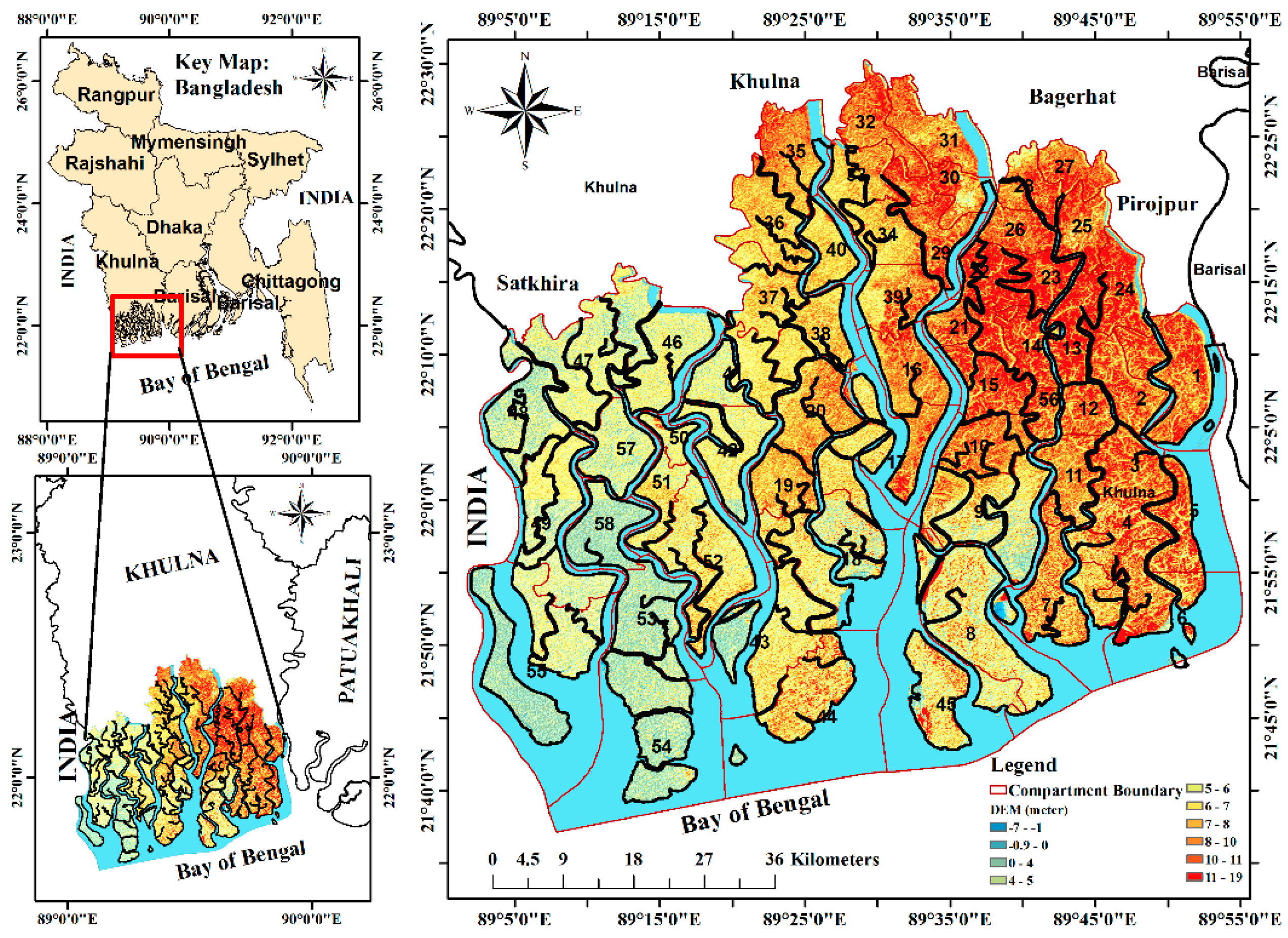
3.1. Study Area

The Sundarbans mangrove forest (SMF) is an unique natural habitat for about 300 species of flora, 425 species of terrestrial fauna and 291 species of fishes [89], and has been recognized as an important natural resource base, due to its geographic location, climatic conditions and species diversity. This forest is considered as the largest mangrove territory in the world, which is shared by Bangladesh and India. In between two countries, more than 60% of the Sundarban ecosystem is in Bangladesh [90]. In 1987, the United Nations Educational, Scientific and Cultural Organization (UNESCO) declared the area as a World Heritage Site officially named as “The Sundarbans” [91] and on 21 May 1992, it was officially named Ramsar Wetland as “Sundarban Reserve Forest” (SRF) [92] and on 30 January 2019, it was also referred to as “Sundarban Wetland” [93]. In this study, we have used SRF as it is well known locally and internationally. The study area lies approximately between 89°2′00″ E to 89°53′00″ E longitude and between 21°37′00″ N to 22°30′00″ N latitude (Figure 1). The entire SRF consists of 601,700.22 ha and shares a major portion with the mangrove forest, including important rivers and numerous tidal creeks. The SRF was categorized into 58 compartments by the Bangladesh Forest Division (BFD) in 1975, and for the protection and monitoring of its valuable resources, it was selected for the present study.

The topographically, SRF is generally flat in nature. The elevation varies locally from west to east, where the western part has a height variation of 0–6 m, in middle section it varies by 5–10 m and in the eastern part it varies by 4–19 m above mean sea level (AMSL). The climate in SRF is generally soothing and pleasant. The temperature ranges from 20–34 °C and the level of rainfall is extremely high, and the weather is almost moist, with hot, humid air (80% humidity) blowing constantly from the Bay of Bengal (BoB) [94]. The forest has economic value; wood is valued as timber (although protected) and the major tree species of the Sundarbans are sundari (Heritiera fomes), goran (Ceriops decendra), gewa (Excoecaria agallocha), keora (Sonneratia apetala), passur (Xylocarpus granatum), kankra (Bruguiera gymnorhiza) and baen (Avicennia officinalis) [93,95,96,97,98]. Tree height variations are observed across the entire SRF, in the south central and northwest regions by 0–5 m, in the southwestern part by 5–10 m and in the north and southeast they vary by 10–15 m [99,100].

3.2. Methods

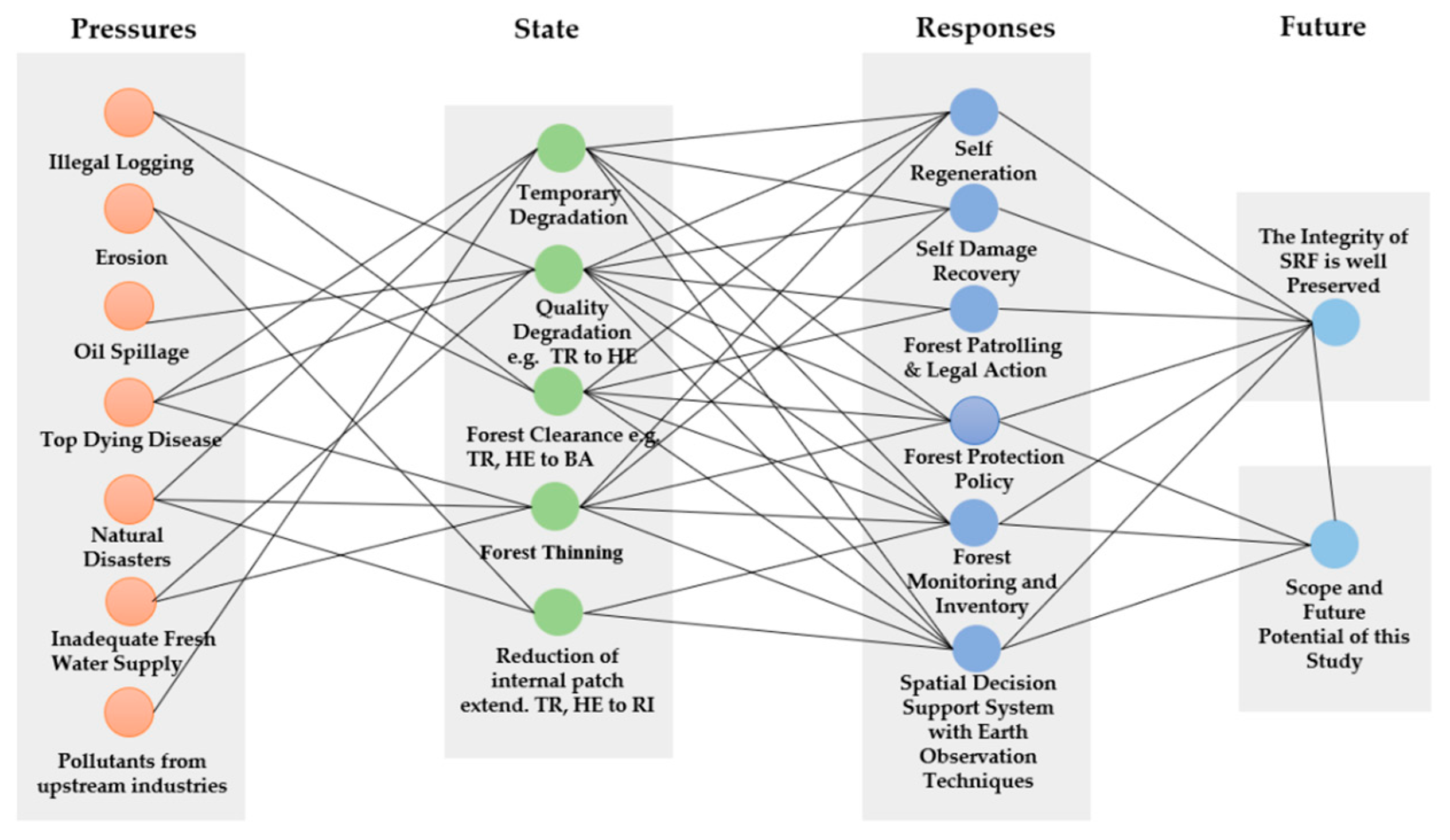
3.2.1. Understanding SRF Changes through PSRF Conceptual Framework

To understand the prediction of forest cover changes and degradation of SRF in Bangladesh, a PSRF conceptual framework was constructed in this study, which was adapted from Liao et al. [48] with modification, exploring multiple drivers of changes, related pressures and the consequences on several states in individual forest compartments of SRF (Figure 2). In this framework, pressures that act upon on SRF changes are due to natural and anthropogenic activities such as illegal logging, top dying disease, oil spillage, pollutants from upstream industries and natural phenomena (e.g., erosion, natural disasters, etc.).

The pressures increase due to the above activities’ impacts on the state of SRF through multifarious actions such as temporary and quality degradation, forest clearance or thinning, etc. However, the responses are signified in forest protection policies, forest monitoring and inventory and spatial decision support systems (SDSSs) with earth observation techniques including self-regeneration and self-damage recovery of mangrove forests. By observing these phenomena, future FC changes and SFD status of SRF can be measured through multi-temporal Earth observation Landsat satellite data. Spatial forest health rank (FHR), constant good patch (GCP) and forest degradation intensity (FDI) measurements were undertaken by considering three equations (see Section 3.2.6) for the first time in a study of SRF (proposed in this study). In this regard, multi-temporal Landsat earth observation data can help us to explore the SRF in qualitative and quantitative ways to better identify the proxies of multiple pressures, and its changing state. Moreover, implementing forest policies, continuous monitoring and forest inventory and SDSSs, as well as self-regeneration and damage recovery, helps responses to succeed and provides a sustainable future to achieve specific targets of UN 2030 SDGs.

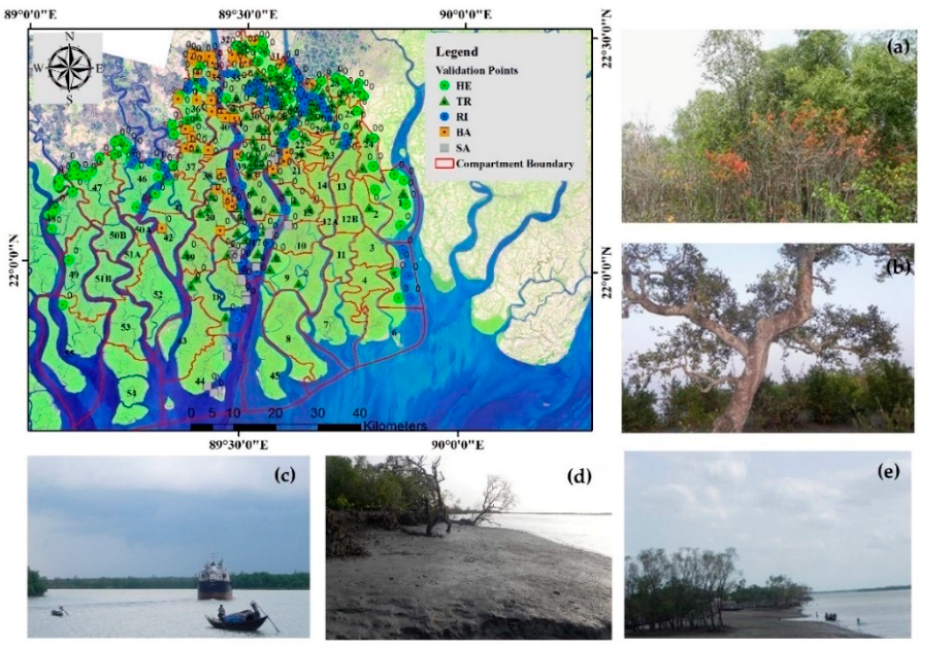
3.2.2. Datasets and Field Survey Data Validation

RS and GIS techniques were used for data acquisition, preparation, data analysis, mapping and reporting. The coupling of RS and GIS along with field survey data is the basis of the study to understand and analyze the present, past and future of the Sundarbans ecosystem. This study uses multi-temporal Landsat imageries at a 30 m spatial resolution for five years (1989, 1999, 2009, 2014 and 2019), to monitor long-term (1989–2019) changes followed by future predictions (2029) in SRF. To advance this, we selected 10 Landsat satellite images in post-monsoon and winter seasons (from November and January) with less than 0.5% cloud cover, including six Landsat 5 Thematic Mapper (TM) and Landsat 7 Enhanced Thematic Mapper (ETM) images and four Landsat 8 Operation Land Imager (OLI) images of path/row 137/45 and 138/45 (see Table S1 for details), acquired from the NASA-USGS EarthExplorer web portal (https://earthexplorer.usgs.gov/) [101]. It is worth mentioning that, to cover broad swathes of the SRF, two Landsat satellite scenes for each sensor in each year were geometrically corrected, mosaicked and projected to the World Geodetic System (WGS) 1984 into the Universal Transverse Mercator (UTM) Zone 45 N and 46 N coordinate system.

Moreover, the other data, such as the SRF administrative boundary and forest inventory data of 1996, were gathered from the Bangladesh Forest Department (BFD) and US Forest Service, respectively. To observe the changes and modeling scenarios, different application software such as ENVI 5.3 (satellite image pre-processing, image enhancement), ERDAS Imagine 2014 (interpretation and classification), TerrSet IDRISI 18.21 (land and FC simulation, projection modeling and transition matrix), ArcGIS 10.7 (GIS data for SFHQ and SFD assessment through FDI mapping and analysis) and Microsoft Excel 2019 (numerical analysis for tables and charts) were used to analyze the various types of data throughout the study.

In addition, field surveys were conducted in the entire SRF in March–April 2015 and February 2018 with forest field officials, maintaining certain limits to access inside the forest to avoid dangerous wild animals such as Bengal tigers, snakes, deer, etc. To conduct the survey, we used available Google Earth (GE) images with a forest compartment layer overlay, along with the Garmin eTrex global positioning system (GPS), including field photos, to collect field validation points of the MF and the surrounding environment. A total of 305 ground validation points were taken across the SRF to use further in image classification accuracy assessments, where 170 points represented MF the categories of Land Use (LU) types as light forest/small trees (HE) and dense forest/large trees (TR) and 135 points represented other LU types as water bodies (RI), bare land (BA) and sandy area (SA) (Figure 3).

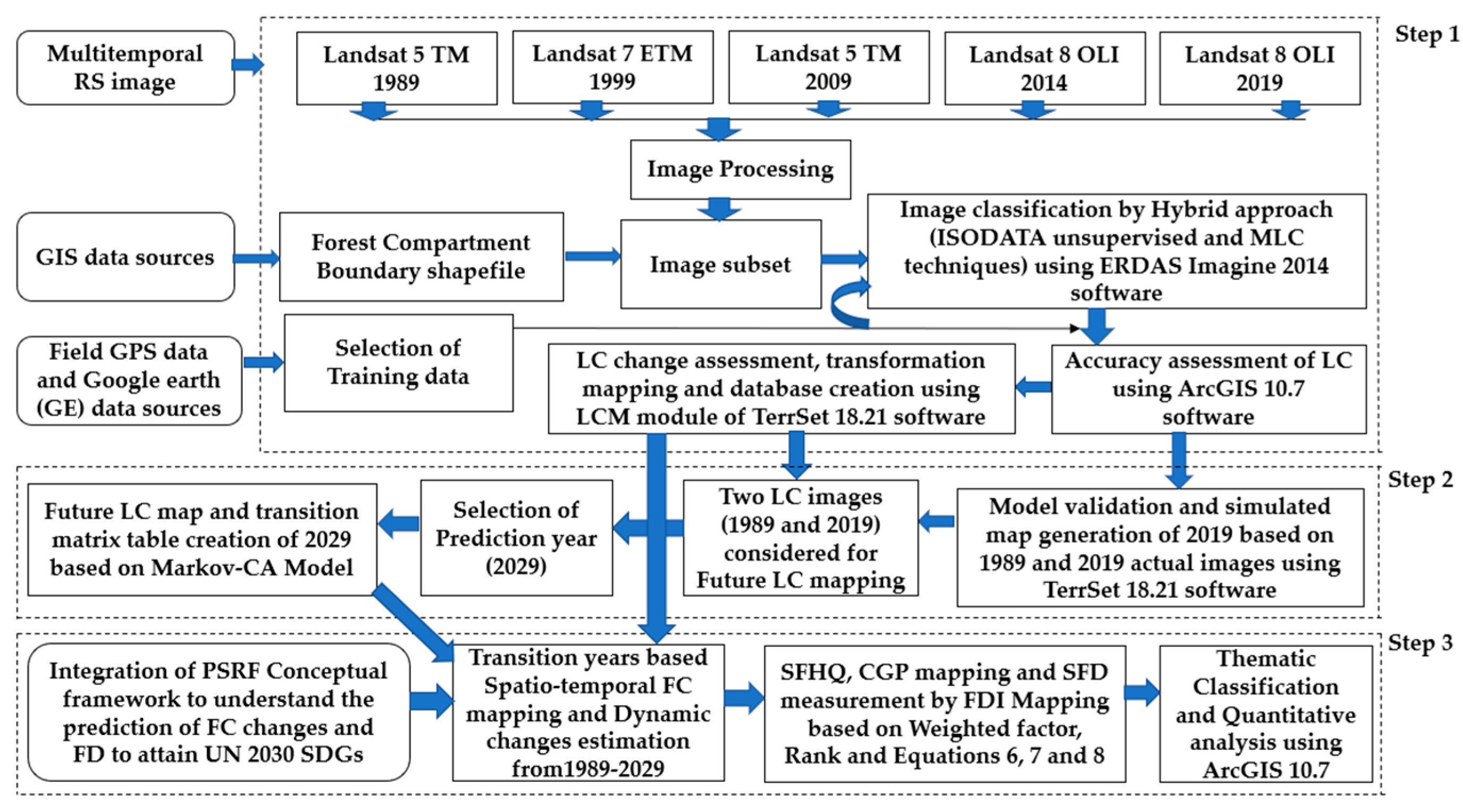
3.2.3. Image Processing, Classification Techniques and LC Mapping Method

In order to fulfill the coverage of the entire SRF of Bangladesh, two satellite scenes for each of the selected years and a total of ten satellite scenes were considered in this study to interpret and analyze the images. The image processing steps involved pre-processing steps first, where Landsat 5 TM, 7 ETM and 8 OLI images were processed by standard procedures such as image calibration to at-sensor radiance, then radiometric correction was performed using an atmospheric correction model to get surface reflectance images. These correction steps were applied to the images using the Fast Line-of-sight Atmospheric Analysis of Spectral Hypercubes (FLAASH) tools based on a MODTRAN radiative transfer module of ENVI 5.3 software. To perform spatial matching between images, image-to-image geometric correction was considered prior to the image interpretation and 5% linear image enhancement algorithms and histogram equalization were applied for better visualization of various features in the Landsat multispectral data.

In this study, we used a hybrid approach, comprising unsupervised and supervised image classification techniques [102] to obtain necessary LC classes in the SRF. Therefore, in the beginning, we collected signatures with an iterative self-organizing data analysis (ISODATA) classification algorithm technique. The ISODATA clustering method is employed to reduce primary human efforts to distinguish between LC classes for the less known and less accessible areas, like SRF, using the spectral separability of the machine itself. The advantage is that the analyst has a prior idea about the probable LC classes of the study area and has the opportunity to confirm any confusing LC classes through field validation. In the hybrid classification process, the ISODATA techniques, along with human-derived training data, yield better accuracy through integrating machine and human skill. The selected clusters were then assigned to specific classes based on field verification before using them as classification training data in ERDAS Imagine 2014. The signatures were evaluated using the histogram technique/transform divergence (TD) to ensure that each signature was normally distributed [103]. In order to achieve a higher accuracy of LC class derivation, we eliminated the signatures that were not normally distributed and had poor TD separability. TD values ranged between 0 and 2000 and a TD above 1500 was considered to be separable. Values greater than 1700 indicated good separability and those above 1900 indicated excellent separability [104]. In our study, a TD value of ≥1900 was found, which indicated an excellent separable category.

After evaluation, we used the retained signatures as inputs and ran a maximum likelihood classification (MLC) in ERDAS Imagine 2014 software to classify spectral signatures into five discrete LC categories, namely: light forest (i.e., seedlings, saplings, herbs and shrubs, small trees, partly degraded forest that has diameter at breast height (dbh) < 15 cm) designated as HE, dense forest (i.e., trees with canopy coverage, continuous patches of trees that have dbh > 15 cm, especially large trees) referred to as TR, water bodies (i.e., ocean, small and large rivers, creeks, swamps) designated as RI, bare land (exposed soil, mudflat, degraded forest) designated as BA and sandy areas (sand or sandy soil) considered as SA. The MLC algorithm has been the most common, popular and widely used classification algorithm for a long time, as the process is very easy and less computational engagement is required [105]. However, as of now, the newly developed artificial neural network (ANN), support vector machine (SVM) and deep learning (DL) algorithms have not been thoroughly compared for MF classification. Therefore, we relied on the MLC technique for our final image classification, and it also provides statistically satisfactory results for a large area compared to the nearest neighbor algorithm.

To support the MLC technique by considering the temporal image dates, field discussion data were collected after discussion with the forest beat officers from major forest compartments of SRF regarding the existence of particular features of LC. Therefore, the ground validation GPS data points and GE high-resolution satellite images were used for signature collection and accuracy checks of the five different LC classes, while the 30 m resolution Landsat scenes were used for classification because of their long temporal availability, which is absent in other sensors such as Sentinel 2A, Sentinel 1 synthetic aperture radar (SAR), hyperspectral and so on. Moreover, to improve the historic data classification, we used visual interpretation of the images by applying false color, infrared, true color and other custom combinations on images to distinguish spectral features. In this regard, the classified 2019 image was used as a reference image for the digital visual interpretation technique (DVIT) of LC classes for images of preceding years. The results were trusted to be accurate because of field validation conducted in SRF. The use of the DVIT in this context is not uncommon and its benefits are reported by other studies [106,107].

In the next step, we categorized LC maps within the GIS programs into HE, TR, RI, BA and SA and maps were prepared with a scale of 1: 500,000. The identified LC pattern was cross-verified within the present context to identify how many losses or gains occurred in the SRF areas. We used the historic data (1989–2019) to project changes in LC, looking 10 years into the future (i.e., 2019–2029). The classified temporal imagery data were used to prepare a geospatial database. The database identified the current state of the LC as well as compared the changes in LC from 1989–2019. In the next step, the 2019 simulation was prepared based on twice classified data (1989 and 2019) in the LCM module of TerrSet version 18.21 software and then the 2029 prediction was made which was considered as a 10-year projection under the business as usual (BAU) scenario of the model. This projection is envisaged to be the working plan of Bangladesh, usually considered for 10 years [108], as well as to facilitate Government of Bangladesh (GoB) in fulfilling the SDGs target which is due by 2030. Moreover, LC change transformations based on different time frames in 1989–2029 were performed in the same software.

3.2.4. Dynamic Degrees (DD) and Transition Matrices Computation Method

At this stage, the DD model was used to represent the spatio-temporal characteristics of LC changes and gain and loss (%) were estimated for earlier and future time period change data. To attain this, DD estimation can be calculated using the approach adopted from Liu et al. [109], and from other researchers [10,33,110,111], as shown in Equation (1):

$$D=\frac{\frac{Ab-Aa}{Aa}}{T}\times 100\%$$

(1)

where D represents the DD model, which refer to rate of change; A_a is the area in the initial year; A_b is the area in the terminal year; and T is the temporal scale. In this study, the time comparisons are 10, 10, 5, 5 (for past), 30 (overall past years), 10 (for future prediction) and 40 years (overall past–future).

Moreover, land cover transition (LCT) maps were generated based on historical and predicted data of different time periods (i.e., 1989–1999, 1999–2009, 2009–2014, 2014–2019, 1989–2019, 2019–2029 and overall 1989–2029), as well as matrix information computed in the LCM module of TerrSet 18.21 software. These LCT data are generally used to identify the transformation of each LC class through a qualitative and quantitative manner [32,33]. At this stage, each LC map was used to observe the change in the next most recent one, to produce a transition matrix for each time period. Based on five LC classes, LCT maps of different time periods were prepared following a from–to approach. In the next step, all time frame raster images were converted into vector form using ArcGIS 10.7 software, which allowed us to identify the areas where changes occurred in the past, as well as what will occur or persist in the future. Finally, all of the results obtained using GIS software were exported to text file and later used for statistical analysis.

3.2.5. Prediction of LC Change Using Markov-CA Model and Simulation Validation

The Markov-CA model is a popular model compared to other modeling approaches, and is generally used for temporal and spatial change estimation [112,113], as well as planning support tools [113]. The Markov-CA model signifies the model as a combination of a Markov chain and cellular automata to predict the LULC trends and characteristics over time [58]. In particular, in geographical research, the Markov chain model was developed by Andrei A. Rakov in 1970, and was first used by Burnham for land use modeling [75,114]. This model provided a simple methodology which dissected a dynamic system and examined LULC change from one time to another [13,29,30,33,34,115,116,117,118,119,120] in order to predict future change [24,25] based on Equation (2):

$$S \left(t, t+1\right)=Pij \times S \left(t\right)$$

(2)

where S(t) represents the status at time t, S(t + 1) is the status at time t + 1 and Pij is the transition probability matrix (TPM) in a state which is calculated based on Equations (3) and (4) [81,88,116]:

$$P_{ij}=\left[\begin{array}{cccc}{P}_{11} & P_{12 }& \dots & P_{1n} \\ P_{21} & P_{22 }& \dots & P_{2n} \\ \dots \dots & \dots \dots & \dots \dots & \dots \dots \\ P_{n1 }& P_{n2 }& \dots & P_{nn} \end{array}\right]$$

(3)

$$(0\le Pij<1)$$

(4)

P is the transition probability; $Pij$ represents the probability of converting from current state i to another state j in next year; P_n is the state probability of any time. A low transition value will have a probability near (0) and a high transition have a probability near (1) [81].

Furthermore, cellular automata (CA) considered with a Markov chain in a model boost LULC modeling, which is a robust approach in spatio-temporal dynamic modeling [88,120]. The CA model is a dynamic spatial process model that is used for LULC changes. Each particular cell has self-characteristics and can represent a parcel of land with a dynamic character [121] which is dependent on the spatial and temporal characteristics of its neighboring cells.

In order to predict the LC changes, we used the integrated Markov-CA model [33] to simulate LC changes by generating a set of matrices and spatial information. In this regard, the land cover change modeler (LCM) program of TerrSet version 18.21 software was used to predict the LC of 2029, which is widely recognized and used by the scientific community to monitor and model earth system processes [33]. Before that, a simulated image of 2019 was generated based on the initial year (1989) and final year (2019) images and then the transition probability matrix (TPM) and transition area matrix (TAM) were prepared from the Markov model. The transition suitability image (TSI) was also generated at this stage, and then all three (TPM, TAM and TSI) were integrated in the Markov-CA model. Finally, a 5 × 5 contiguity filter was applied with five iterations to model the LC for the year 2029 to visualize the significant cellular changes, and then the TPM of future LC classes in specific time period (such as 2019–2029) was obtained using the Markov model.

In addition, the model needed to be validated further with the LC image of 2019 (derived from the Landsat 30 m image) by using chi-squared (χ²) test statistics and the kappa index of agreement with goodness of fit. Therefore, simulated image of 2019 was compared with the 2019 actual image (Landsat 8 OLI) and the result was hypothetically tested, as the area statistics of both images were the same. This is valid when the test statistics are χ² distributed under the null hypothesis, specifically Pearson’s ${\mathsf{\chi }}^2$ test and variants thereof, and the test is done with the following formula:

$${\mathsf{\chi }}^2=\sum {\left(\mathrm{O}-\mathrm{E}\right)}^2/\mathrm{E}$$

(5)

where ${\mathsf{\chi }}^2$ denotes chi-squared, O is the observed image (in our case, simulated LC image 2019) and E is the expected image (in our study it is the actual LC image 2019).

However, this does not necessarily validate the agreement on the spatial distribution of the LC classes of the study site. To solve this problem, we performed a more sophisticated kappa index of agreement between the two images. Moreover, the kappa coefficient value was measured [10,32,121,122,123] using the following set of conditions: <0 = less than chance agreement, 0.01–0.40 = poor agreement, 0.41–0.60 = moderate agreement, 0.61–0.80 = substantial agreement and 0.81–1.00 = almost perfect agreement. In the kappa index, three indicators were used for the Markov-CA model validation, kappa for no ability (k_no), kappa for location (k_location) and kappa for quantity (K_quantity), which is strongly recommended [124]. The accuracy of the LC classification is very crucial to assess and understand the statistical significance of the classification. According to Eastman [125], the simulation is well justified with an acceptable accuracy rate of 0.80 (which is within the conditions 0.61–0.80 = substantial agreement) and is considered for plausible future predictions, where a value of the indicator equal to 1 is well defined and it is unsatisfactory when it is equal to 0 [36,126].

3.2.6. Assessment Method of SFHQ and SFD

In order to assess qualitative and quantitative SFHQ and SFD in forest degradation intensity (FDI) scenarios, three equations were considered (proposed in this study) to observe the past and future condition of SRF. Before FD change assessment, SFHQ and Constant Good Patch (CGP) assessments are also necessary to clearly understand the FD status. In these aspects, the SFHQ value ranges from 0 to 10, where the higher the value, the higher the forest quality and vice versa, which is also similar for CGP. However, the individual SFD map is prepared based on the FDI whose rank is defined as -10 to +10, where, ‘−’ value represents forest improvement or regenerations and ‘+’ value represents forest degradation. This rank is assigned based on the improvement and degradation percentage such as −1 to 6 in the present study, where −5–−14% degradation is −1, rank 0 is −4–5%, rank 1 is 6–15% FD, 16–24% is rank 2, 25–34% is rank 3, 35–44% is rank 4, 45–54% is rank 5 and 55–64% FD is rank 6. In this case, the lower the FDI value, the healthier the forest is. To prepare SFHQ, CGP and FDI maps, past and future scenario statistics were calculated based on the following three equations with Microsoft Excel 2019 and ArcGIS 10.7 software environments, respectively.

$$\mathrm{SFHQ}=\mathrm{WTR}\times \left( \frac{100\times \mathrm{TR}}{\mathrm{CA}-\mathrm{RI}}\right)÷100+\mathrm{WHE}\times \left(\frac{100\times \mathrm{HE}}{\mathrm{CA}-\mathrm{RI}}\right)÷100$$

(6)

where SFHQ = spatial forest health quality, WTR = weighting value for TR (10 in this study), TR = TR area in particular compartment in an assessment year, CA = compartment area, RI = water Area in particular compartment in an assessment year, WHE = weighting value for HE (five in this study).

$$\mathrm{CGP}=\frac{\mathrm{FQy}1+\mathrm{FQy}2+\mathrm{FQyn}}{\mathrm{yn}}$$

(7)

where CGP = constant good patch, FQyn = forest quality for particular year (In this study, six years).

$$\mathrm{FDI}=\frac{\left\{\left(\mathrm{TRG}-\mathrm{TRL}\right)+\left(\mathrm{HEG}-\mathrm{HEL}\right)\right\}\times 100\times \mathrm{WV}}{\left(\mathrm{CA}-\mathrm{RI}\right)\times 100}$$

(8)

where FDI = forest degradation intensity; TRG = gain of TR (transitioned total from HE, RI, BA and SA); TRL = loss of TR (transitioned total from HE, RI, BA and SA); HEG = gain of HE (transitioned total from RI, BA and SA); HEL = loss of HE (transitioned total from RI, BA and SA); WV = weighted value for DI rank; CA = compartment area; and RI = water area in a compartment. Moreover, the detailed integrated methodological flowchart of the research process considers three main steps, which is shown in Figure 4.

4. Results

4.1. Accuracy Assessment of LC Classification Images and Validation of Future LC Projection

Table 1. The producer, user and overall accuracies of 5 TM (1989), 7 ETM (1999), 5 TM (2009), 8 OLI (2014, 2019 act., 2019 sim.) images using MLC techniques.

Landsat Sensors	Time	Val. Points	HE		TR		RI		BA		SA		Accuracies
			PA (%)	UA (%)	PA (%)	UA (%)	PA (%)	UA (%)	PA (%)	UA (%)	PA (%)	UA (%)	OA (%)	Kappa
TM	1989	305	72.86	77.27	86.00	85.15	97.14	97.14	93.33	84.00	90.00	100.00	86.89	0.82
ETM	1999	305	70.00	69.01	81.00	81.00	98.57	98.57	91.11	91.11	95.00	100.00	84.92	0.79
TM	2009	305	82.86	77.33	86.00	89.58	95.17	98.53	88.89	83.33	85.00	94.44	87.87	0.83
OLI	2014	305	80.00	82.35	91.00	89.22	98.57	97.18	88.89	85.11	85.00	100.00	89.51	0.85
OLI	2019 (act.)	305	85.71	81.08	87.00	91.58	97.14	98.55	93.33	87.50	95.00	100.00	90.49	0.87
OLI	2019 (sim.)	305	77.14	62.79	77.00	83.70	92.86	97.01	84.44	88.37	85.00	100.00	82.30	0.75

Note: TM: Thematic Mapper; ETM: Enhanced Thematic Mapper; OLI: Operation Land Imager; Val. Points: Validation points; PA: Producer’s accuracy; UA: User’s accuracy; OA: Overall accuracy; HE: Light forest; TR: Dense forest; RI: River; BA: Barren area; SA: Sandy area; MLC: Maximum likelihood classification.

summarizes the producer accuracy (PA), user accuracy (UA), overall accuracy (OA) and finally Cohen’s kappa coefficient [127] of the various LC classes of SRF for LC maps for the time periods of 1989, 1999, 2009, 2014, 2019 (actual) and 2019 (simulated). The results revealed among all the images that the highest OA and kappa statistics were found for the 2019 supervised classification at 90.49% and 0.87, respectively.

However, a detailed classification matrix is given in Supplementary Table S2a–f, where the rows denote the categories derived from the classified image, and columns represent the categories identified from the reference values [121,128,129]. The diagonal of the matrix shows the agreement of the “from–to” categories identified from the reference values. On the other hand, the off-diagonal represents the disagreement of the “from–to” categories which indicates the errors (omission and commission errors) that remain between the classified and reference data [130]. In connection with this, the actual LC of 2019 was compared with the simulated 2019 LC based on the Markov-CA model. This model is further validated by the chi-squared (χ²) test result generated based on Formula (5) of Section 3.2.5. The generated data and the graphical illustration are given in Table S3 and Figure S1, respectively. The tabulated chi-squared (χ²) value was found to be greater (χ² _0.975 ⁽⁴⁾ = 0.484) than the calculated one (0.335), so, we failed to reject the null hypothesis. Although the above result does not necessarily validate the agreement on the spatial distribution of LC classes of the study area, a similar kind of validation problem was also observed by Nath et al. [33]. By observing this issue, a more sophisticated standard kappa index of agreement between two images with goodness of fit, which is corrected for accuracy by chance [131], is performed in the LCM module of TerrSet 18.21 software and further partitions the agreement/disagreement components (see Table S4) into 0.0444 (error due to quantity/disagree quantity) and 0.1585 (error due to allocation/disagree grid cell). However, the main disagreement was due to an allocation error rather than quantity errors between simulated and actual 2019 LC images. At this stage of validation, the Markov-CA model was a good fit to run the future prediction of the LC.

Moreover, the overall accuracy of the projection model could be further obtained from the Kno index, which is the standard kappa index of agreement. The Klocation index validates the ability of the simulation to predict the location. Based on the all indices of agreement results (Table S4 for details), the average value was found to be 0.76, which means that the LC categories of the actual and simulated images were more than 75% similar, which indicates substantial agreement. Therefore, finally, the model is ideally fit for future predictions of SRF.

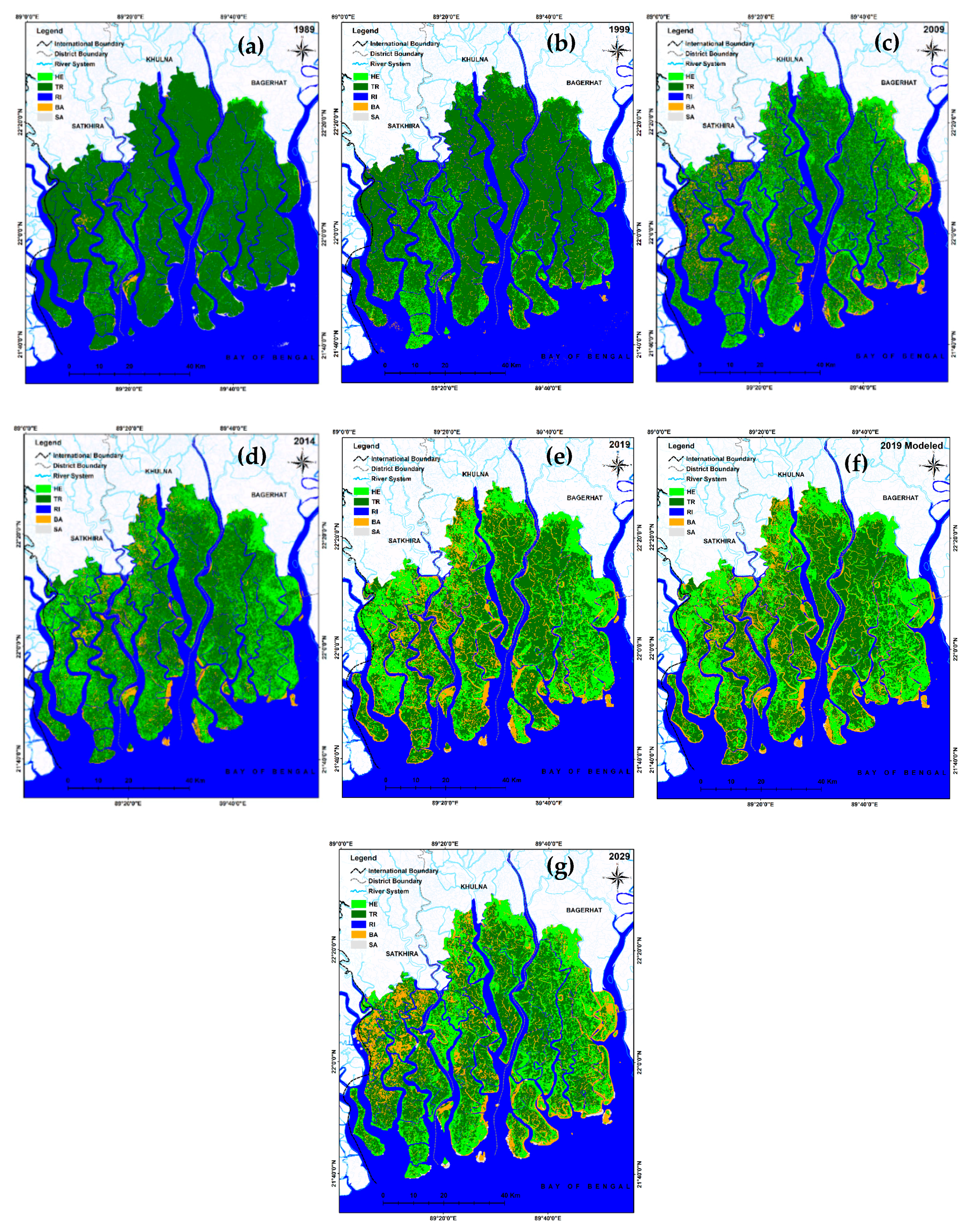
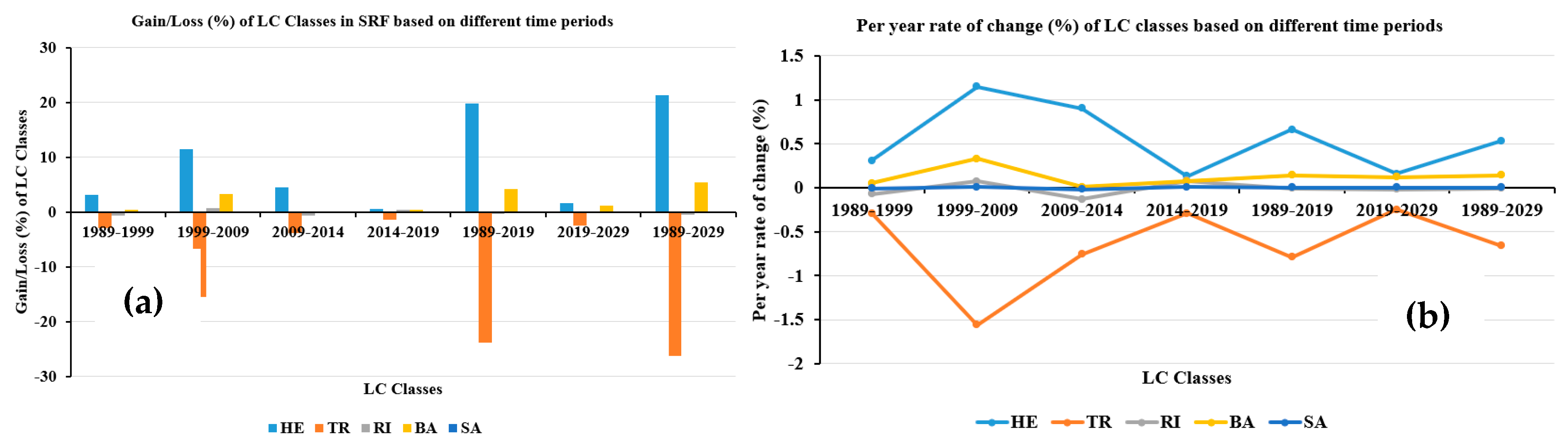
4.2. Historical and Future LC Change Analysis of SRF

In the classified LC images, deep green patches indicate TR, while light green patches indicate the regeneration of plants as HE, whereas BA and SA were identified in almost all adjoining areas of tidal creeks, highlighted with orange and white, as observed in the western, southern and eastern parts of the SRF. Tidal river, creeks and ocean parts of the Bay of Bengal (BoB) were considered as RI.

The LC areal changes of SRF from 1989–2029 are presented in Figure 5a–g, and statistics are presented in

Table 2. Types of LC within the SRF from 1989 to 2019 presented in hectares and percentages, based on multi-temporal satellite data.

LC Categories	1989		1999		2009		2014		2019 (Actual)		2019 (Simulated)		2029
	Area (ha)	%	Area (ha)	%	Area (ha)	%	Area (ha)	%	Area (ha)	%	Area (ha)	%	Area (ha)	%
HE	30,069.27	5	48,884.76	8.12	118,139.49	19.63	145,268.1	24.14	149,181	24.79	150,909.48	25.08	158,424.66	26.33
TR	364,686.93	60.61	347,400.81	57.74	253,201.14	42.08	230,281.83	38.27	221,496.3	36.81	220,685.67	36.68	206,410.95	34.31
RI	196,132.77	32.6	191,995.29	31.91	196,140.24	32.6	192,134.88	31.93	194,556.51	32.33	192,172.77	31.94	193,591.71	32.17
BA	10,168.47	1.69	13,183.65	2.19	33,310.08	5.54	33,584.76	5.58	35,866.35	5.96	37,560.33	6.24	42,835.5	7.12
SA	642.78	0.11	235.71	0.04	909.27	0.15	430.65	0.07	599.22	0.1	371.97	0.06	437.4	0.07
Total	601,700.22	100	601,700.22	100	601,700.22	100	601,700.22	100	601,700.22	100	601,700.22	100	601,700.22	100

Source: USGS EarthExplorer for Landsat 5 TM, 7 ETM and 8 OLI Satellite images from 1989–2019 and, based on 1989 and 2019 images, 2019 simulated and prediction images for 2029 were generated; data extraction and compilation was done by the JDR 3rd Research Mangrove Team using ERDAS 2014 and ArcGIS 10.7 software.

.

The results indicate that changes in LC patterns of SRF started in 1989, which had 394,756.20 ha of forests, with the majority being TR (60.61% of all the land) (Table 2 and Figure 5a), while in 1999, there was HE on the western and southwestern margins of the SRF. The proportion of BA increased slightly in 1999 (Table 2). FD started to become visible along the southern coast of the SRF, due to river and seawater influences (one of the drivers), although regeneration of mangrove species took place in some parts of the SA through successional processes (Table 2 and Figure 5b).

In 2009, the proportion of TR showed a downtrend (42.08%), while the proportions of HE (19.63%), RI (32.60%), BA (5.54%) and SA (0.15%) were enhanced significantly (Table 2 and Figure 5c). On the other hand, in 2014, the LC status suggests improvements in the HE (24.14%) areas due to self-regeneration (natural causes) of the SRF in the forest compartments (Table 2 and Figure 5d). The FC in SRF was severely affected due to two successive natural disasters, super cyclones Sidr in 2007 and Aila in 2009, with an overall decline in TR, which remained as 38.27% (Table 2 and Figure 5d). However, the TR in the 2019 actual image is 36.81%, (Table 2 and Figure 5e) a sharp decrease compared to the 2014 status (38.27%). However, HE is almost the same as in the 2019 actual image (24.79%) and in 2014 (24.41%) (Table 2 and Figure 5e,d). The LC of the TR area is almost similar up to 36.68% in 2019 (simulated) (Figure 5f) compared to the 2019 actual state (36.81%) (Table 2 and Figure 5d), whereas it will be 34.31% (Table 2), showing less TR by the year 2029 (Figure 5g) with deterioration of up to 2.5%. Moreover, a greater proportion of HE (26.33%), RI (32.17%) and BA (7.12%) will be present in 2029 (Table 2 and Figure 5g) and the southwestern part of the forest will incur significant losses in this regard. The results also suggest that HE will be in an uptrend by up to 1.54% by the year 2029 (calculated based on Table 2).

In addition, there will be a slight downtrend in the areas of RI by 2029, suggesting that erosional activities (one of the causes of SRF changes) will continue in the future. Moreover, BA areas were slightly enhanced in both 2019 actual and simulated images (Table 2 and Figure 5e,f) because of natural regeneration activities (common in the mangrove tidal flat areas across the world). However, the prediction of the year 2029 indicates that higher portions of BA are projected in the western, eastern, southeastern and northern parts of the SRF (Figure 5g).

However, the different time period comparison results reveal that important changes occurred in the SRF (

Table 3. LC change assessment of the SRF based on different time frame data (1989 to 2029).

LC Classes	Land Cover Change (1989–1999)
	Magnitude Area (ha)	% Change	Annual Rate of Change (ha yr−1)
HE	18,815.49	62.57	1881.55
TR	−17,286.12	−4.74	−1728.61
RI	−4137.48	−2.11	−413.75
BA	3015.18	29.65	301.52
SA	−407.07	−63.33	−40.71
LC Classes	Land Cover Change (1999–2009)
	Magnitude Area (ha)	% Change	Annual Rate of Change (ha yr−1)
HE	69,254.73	141.67	6925.47
TR	−94,199.67	−27.11	−9419.97
RI	4144.95	2.16	414.49
BA	20,126.43	152.66	2012.64
SA	673.56	285.76	67.36
LC Classes	Land Cover Change (2009–2014)
	Magnitude Area (ha)	% Change	Annual Rate of Change (ha yr−1)
HE	27,128.61	22.96	5425.72
TR	−22,919.31	−9.05	−4583.86
RI	−4005.36	−2.04	−801.07
BA	274.68	0.82	54.94
SA	−478.62	−52.64	−95.72
LC Classes	Land Cover Change (2014–2019)
	Magnitude Area (ha)	% Change	Annual Rate of Change (ha yr−1)
HE	3913.74	2.69	782.75
TR	−8785.53	−3.81	−1757.11
RI	2421.63	1.26	484.33
BA	2281.59	6.79	456.32
SA	168.57	39.14	33.71
LC Classes	Land Cover Change (1989–2019)
	Magnitude Area (ha)	% Change	Annual Rate of Change (ha yr−1)
HE	119,112.57	396.13	3970.42
TR	−143,190.63	−39.26	−4773.02
RI	−1576.26	−0.80	−52.54
BA	25,697.88	252.72	856.60
SA	−43.56	−6.78	−1.45
LC Classes	Land Cover Change (2019–2029)
	Magnitude Area (ha)	% Change	Annual Rate of Change (ha yr−1)
HE	9242.82	6.19	924.28
TR	−15,085.35	−6.81	−1508.53
RI	−964.80	−0.49	−96.48
BA	6969.15	19.43	696.91
SA	−161.82	−27.00	−16.18
LC Classes	Land Cover Change (1989–2029)
	Magnitude Area (ha)	% Change	Annual Rate of Change (ha yr−1)
HE	128,355.39	426.86	3208.88
TR	−158,275.98	−43.40	−3956.90
RI	−2541.06	−1.29	−63.53
BA	32,667.03	321.26	816.67
SA	−205.38	−31.95	−5.13

Note: (I) Land Cover (LC) Changes assessment based on interim years from 1989 to 1999, 1999 to 2009, 2009 to 2014, 2014 to 2019 and 2019–2029 and overall 1989 to 2019 and 1989–2029; (II) (+) sign denotes an uptrend and (−) sign denotes a downtrend of the magnitude of change of LC categories in different time frames.

). In 1989–1999, the most negative change was observed for SA (−63.33%) with −40.71 ha yr⁻¹ and TR (−4.74%) with a rate of change of −1728.61 ha yr⁻¹, while a positive change was observed for HE (62.57%), with a rate of change of 1881.55 ha yr⁻¹, compared to BA (29.65%), which changed by 301.52 ha yr⁻¹ (Table 3). Moreover, RI changed (−2.11%) by −413.75 ha yr⁻¹ (Table 3) due to land erosion (one of the causes) which was relatively higher in the Khulna range, compared to other places across the SRF. This results also support the study conducted by Emch et al. [132] on mangrove FC change detection in the Bangladeshi Sundarbans from 1989–2000 using an RS approach.

In 1999–2009, a negative change was observed only for TR (−27.11% with annual rate of change of −9419.97 ha yr⁻¹) because of the two severe super cyclones that struck in 2007 and 2009 (a major natural cause of mangrove forest changes), which was a bit higher compared to 1989–1999 (Table 3). However, a few significant enhancements were observed for HE and other categories due to an increase in erosion (another major cause) in 1999–2009 compared to 1989 –1999 (Table 3). In 2009–2014, the magnitude of negative change was higher for SA (−52.64% with a change of −95.72 ha yr⁻¹) and TR (−9.05% with a change of −4583.86 ha yr⁻¹) compared to changes in RI (−2.04% with a change of −801.07 ha yr⁻¹), which were lower compared to the other two time periods (i.e., 1989–1999 and 1999–2009). Moreover, the study also observed that the regeneration rate of mangrove species increased across the SRF during the time period of 2009–2014, and severe FD took place in the TR areas, due to the overdependence of local people on forest resources for their livelihood, including illegal logging (one of the major causes of SRF changes). However, the FD continued till the 2014–2019 period with a negative change of −8785.53 ha (−3.81%) and an annual rate of change of −1757.11 ha yr⁻¹ (Table 3). Moreover, the proportion of BA in the SRF in 2014–2019 was boosted by 6.79% compared to 0.82% in 2009–2014 (see Table 3), perhaps due to resource extraction across all forest compartments, which was noticeable in the southeastern part of the SRF.

The area covered in RI also underwent changes in the overall (1989–2019) time period, indicating erosion and accretion of land in the SRF. Looking at the overall change over 30 years, the SRF has been degraded significantly in a negative manner (−4773.02 ha yr⁻¹) with regard to TR (considered as a GFD) and, on the contrary, HE and BA were significantly boosted in a positive way by 3970.42 ha yr⁻¹ and 856.60 ha yr⁻¹, respectively (Table 3). However, the scenario of 2019–2029 (10 years into the future) has a negative trend for TR (−1508.53 ha yr⁻¹), including RI and SA, and, conversely, the HE changes will be in positive a trend of 924.28 ha yr⁻¹, which is comparatively slower (changed by 3970.42 ha yr⁻¹) with respect to the 30 years before (1989–2019) (Table 3). Finally, in the 40-year (1989–2029) time period, TR is going to be changed by −158,275.98 ha (−43.20%) with an annual rate of change of −3956.90 ha yr⁻¹, a greater indication of GFD in SRF. Further, the descriptive statistics results suggest a major share of HE (DD with 12.80% uptrend) in 1989–2019 (30 year-time period), while it had a 14.17% and 6.26% uptrend in 1999–2009 and 1989–1999, respectively (

Table 4. Dynamic degrees (DD) (%) estimation between different times (1989–2029) based on LC total area coverage (ha) (adopted from Table 3).

		DD (%) between Different Times
LC Classes	1989–1999	1999–2009	2009–2014	2014–2019	1989–2019	2019–2029	1989–2029
HE	6.26	14.17	4.59	0.54	12.80	0.62	10.67
TR	−0.47	−2.71	−1.81	0.76	−1.35	−0.68	−1.09
RI	−0.21	0.22	−0.41	0.25	−0.04	−0.05	−0.03
BA	2.97	15.27	0.16	1.36	11.89	1.94	8.03
SA	−6.33	28.58	−10.53	7.83	−1.00	−2.70	−0.80

Note: The LC class definitions are available in Section 3.2.2. Source: Image statistical results calculated by authors considering Equation (1), as shown in Section 3.2.4.

), alternatively representing the FD status in SRF. Moreover, the DD change in SA was observed to be negative (−10.56%) in 2009–2014 which indicates that the transformation occurred in various forest compartments.

The DD change % was positive in all LC classes in SRF in 2014–2019 (Table 4), probably due to forest self-regeneration activities. The SRF showed a higher dynamic degree (DD) in BA (1.94%) from the predicted time period (2019–2029), compared to other LC classes, suggesting more river erosion and severe cyclone-induced damage (a major pressure and identified known causes in the SRF). As a result, forest loss will be incurred in the future which will impact SRF to a greater spatial extent. However, the case was different for LC in 2009–2014, and a faster rate of negative impact was observed upon the TR. This scenario was observed while we performed forest surveys in the major compartments of SRF (see Figure 3a–e for field evidence photo). Moreover, in 2019–2029, the HE and TR area will change in a positive and negative DD with changes of 0.62% and −0.68%, respectively (Table 4), whereas overall from 1989–2029 (40 years), HE and TR will have positive and negative DD trends (0.62%, −1.09%), similar to 2019–2029, but with different DDs (10.67%, −1.09%), respectively. These data suggest that TR will continuously be degraded till 2029, if any protections for forest loss, illegal encroaching, river erosion control, etc., are not executed at the earliest opportunity.

In the next, the gains and losses (%) and per year rate of change (%) of different LC classes in SRF during different time periods (1989–2029) are presented in Figure 6a,b, respectively. The overall HE gain will be 1.59% (0.16% yr⁻¹) (Figure 6a,b) indicating an uptrend scenario through natural regeneration or plantation activities, while there will also be a negative (−0.25% yr⁻¹) downtrend tendency of TR during 2019–2029 (10 years into the future). This scenario alternatively suggests that more dependency on TR forest cover products through illegal logging, encroachment, tree felling, etc., will be the prime causes to aggravate the condition till 2029, resulting in GFD in the SRF. However, in the 40-year period (1989–2029), the rate of change per year was positively higher (21.33%) compared to other LC types (see Table S5 and Figure 6b).

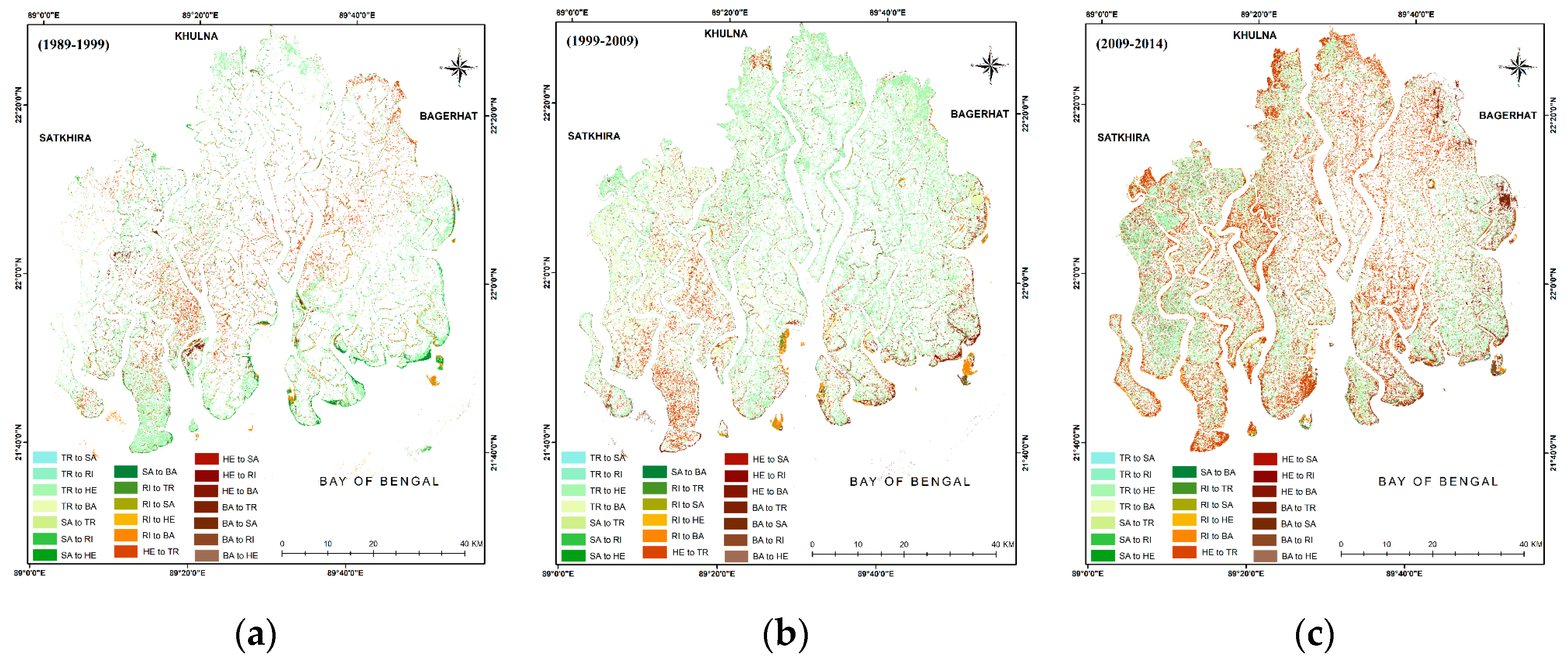
4.3. LC Transition Mapping, Transition Areas and Probability Matrix Analysis (1989–2029)

The LCT mapping for 1989–1999, 1999–2009, 2009–2014, 2014–2019, 2019–2029,1989–2019 and 1989–2029 were prepared and are presented in Figure 7a–g and the cross tabulation matrices are summarized and shown in Table S9 (for details).

Further, TAM and TPM are two important components considered for projection simulation. From the matrix (Tables S5 and S6), it was observed that almost 512,913.0 pixels were expected to be transformed into HE from the TR class during the period of 1989 to 1999. Similarly, 911,462.0, 894,392.0, 896,812.0 and 592,288.0 pixels were expected to be transformed in the same way in four different time periods, 1999–2009, 2009–2014, 2014–2019 and 1989–2019, respectively (see Table S5 for details).

The Future Land Cover (FULC) data of 2019–2029 indicate that the TR class would change to HE and BA, with a probability of (0.2387, 23.87%) and (0.0598, 5.98%), respectively (Table S6), which indicates the future deterioration of FC in the SRF areas. The highest level of LC transformation is observed in HE, with a TP of (0.3303) 33.03% of being transformed into other classes.

Moreover, the LC transformation matrices and spatial change maps of TR to HE in 1989–2029 are shown in Figure S2a–g. The five earlier different time assessment transformation data and maps of 1989–1999, 1999–2009, 2009–2014, 2014–2019 and 1989–2019 suggest that the SRF regions have continuously changed in the past, especially TR to HE conversions (see Figure S2a–g as reference images), which will be maintained into the future till the predicted time (2019–2029), if no action is taken immediately.

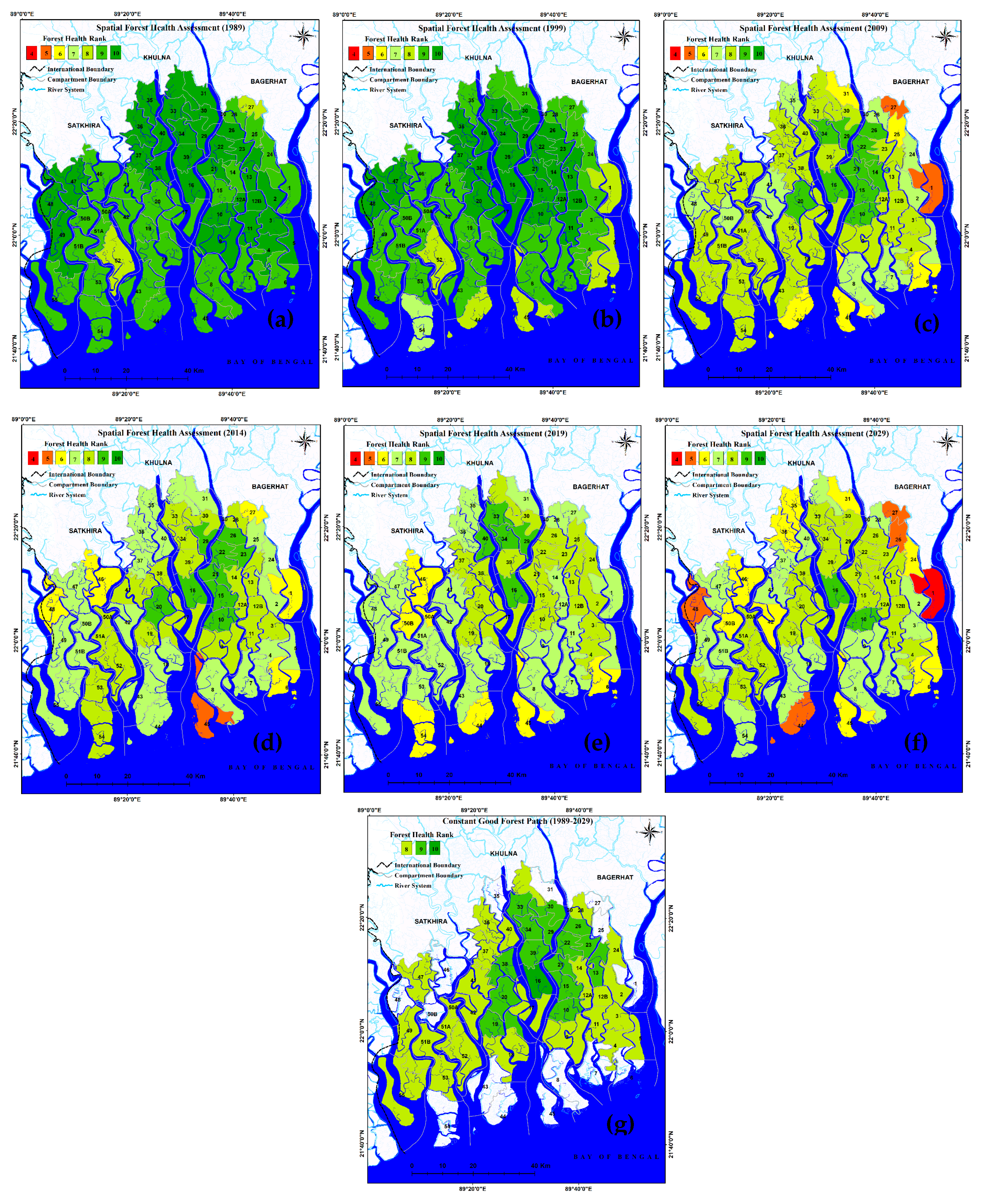
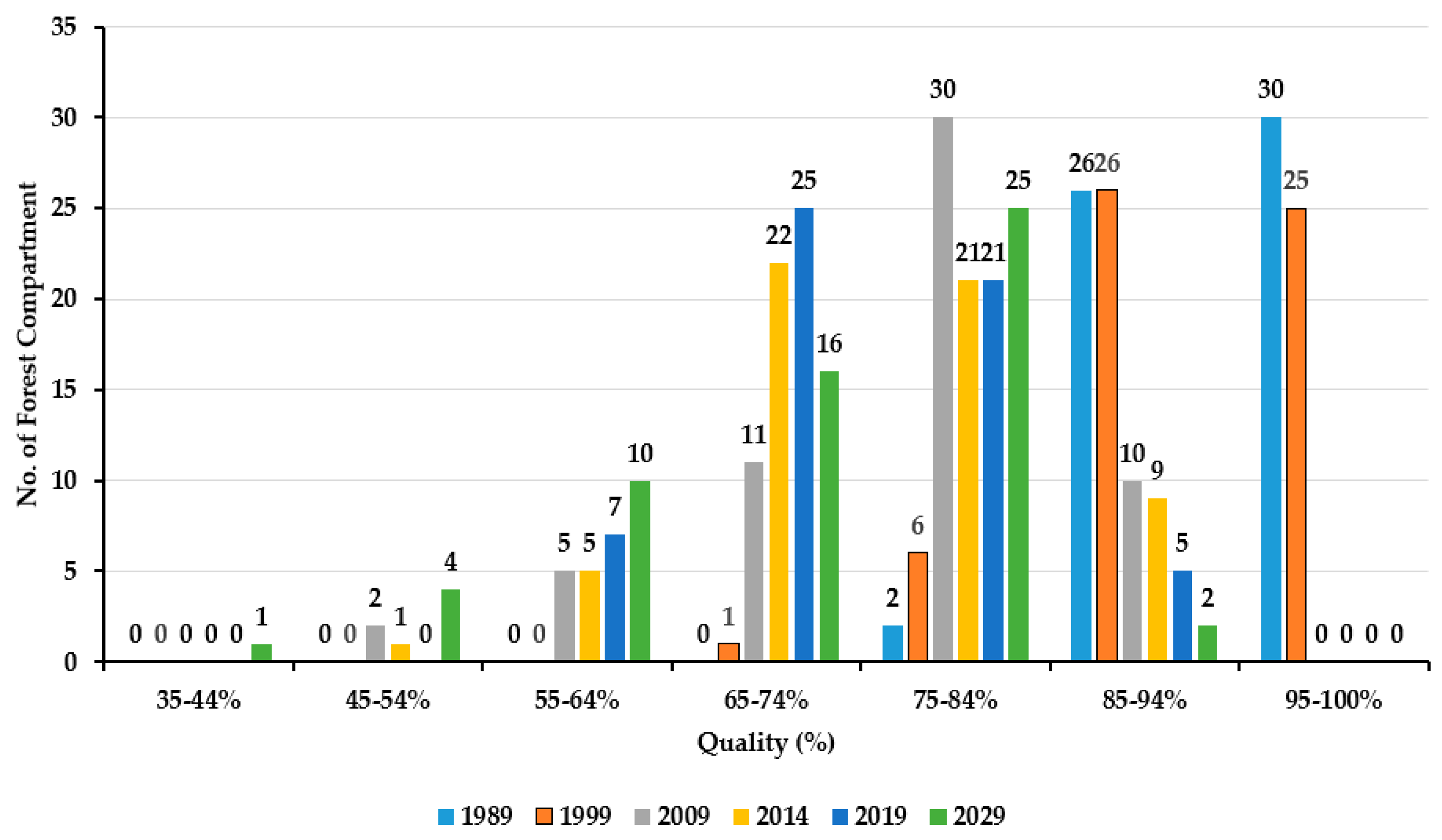
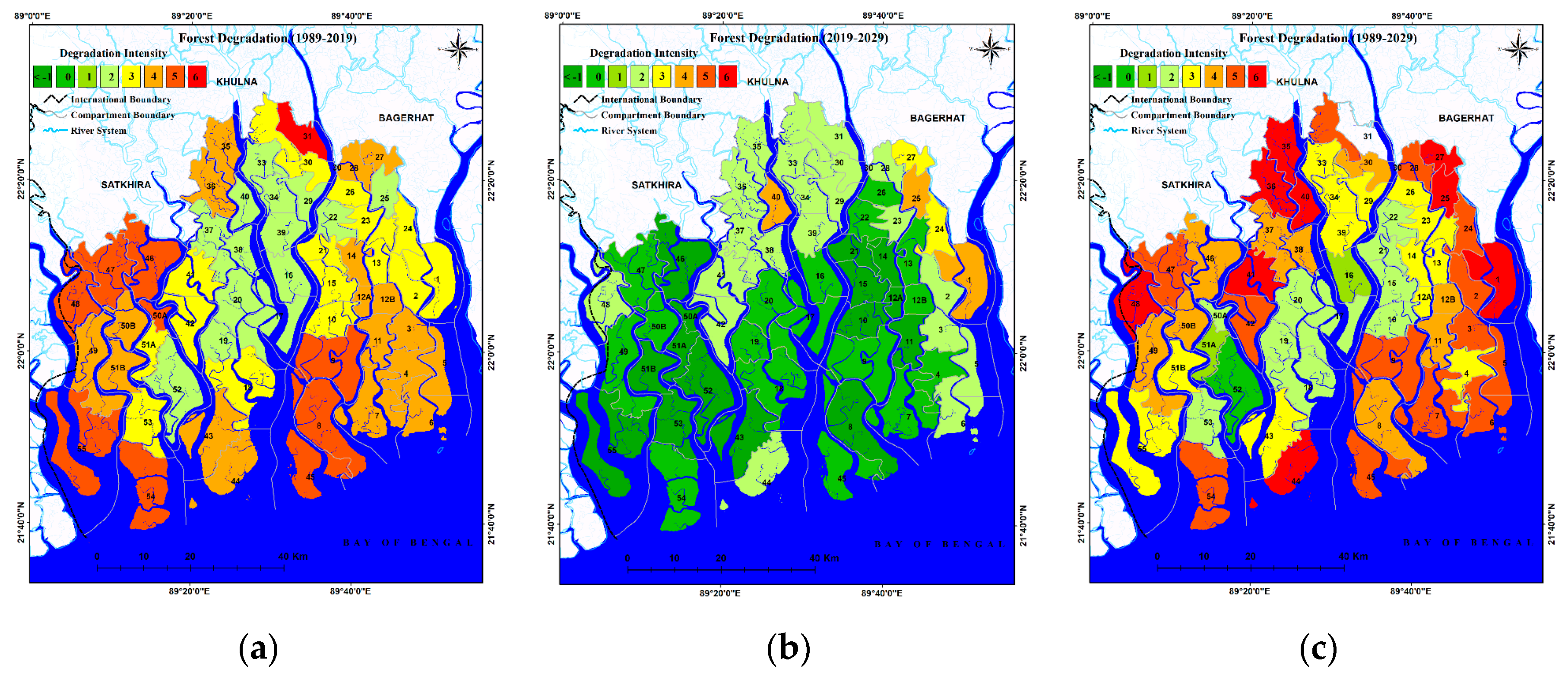
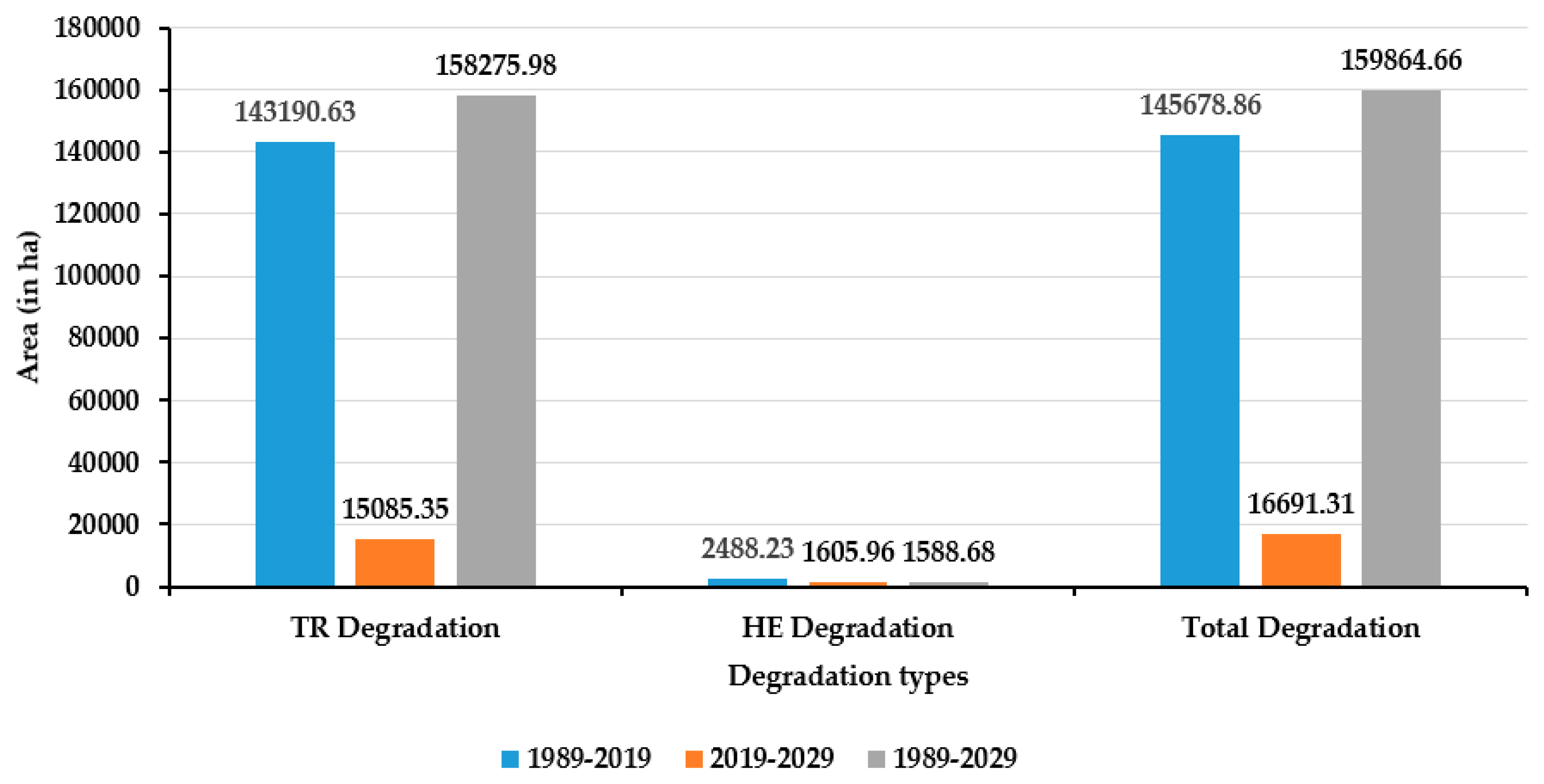
4.4. SFHQ and SFD Assessment (1989–2029)

Changes in SFHQ and SFD of SRF at the spatio-temporal scale from 1989 to 2029 and its corresponding quantitative analyses were prepared based on the considered Equations (6)–(8) (discussed in Section 3.2.6), are shown in Figure 8a–g and Figure 9, respectively. Furthermore, SFHQ and SFD were considered for and are shown in Figure 10a–c and Figure 11, respectively.

Figure 8a–e represent the earlier SFHQ of SRF, whereas Figure 8f,g represent future forest quality and CGF status. The SFHQ values by the number of forest compartment are represented by Figure 9. In 1989, a total of 30 and 26 forest compartments were in good quality, representing 95–100% and 85–94% of TR and HE, compared to the 2019 status, which had five forest compartments with 85–94% quality forest coverage, with no forest compartments classified as top quality forest coverage.

Moreover, 65–74% and 75–84% quality forest was identified in 25 and 21 forest compartments, respectively, which was absent during 1989, because of the presence of good quality forest in that time. These statistics indicate that the SFHQ of SRF was deteriorating significantly between 1989 and 2019 (Figure 8a,e). However, in the interim time period from 1999 to 2014 (Figure 8b–d), quality forest was limited because of degradation, illegal encroachment and other pressures that acted upon SRF. In the future time period (2029) (Figure 8f), the quality of forest will deteriorate further, where only 25 forest compartments will remain in medium to good condition (75–84%), and 16 forest compartments will be 65–74% quality forest, and the remaining forest compartments will be in poor to moderate condition. However, the SRF will maintain a few CGPs of forest (Figure 8g) with rank 8, 9 and 10, meaning 75–100% quality forest (Figure 9), based on the calculated data derived from Equation (7) of Section 3.2.6. The CGP map represents the overall scenario of SRF in the 1989–2029 time period (Figure 8g).

Finally, the SFD maps (in three time domains) were prepared based on Equation (8) of Section 3.2.6, as shown in Figure 10a–c. There are three FDI maps representing the past, future and overall scenarios of the FD status of SRF. The 30-year time period data (1989–2019) (Figure 10a) suggest that SRF underwent a critical stress condition, and it was difficult to maintain its pure, healthy, sustainable forest status due to multiple pressures that are pronounced in SRF (see conceptual framework of Section 3.2.1). In this study, the future time period (2019–2029) (10 years in this study) was considered specifically in which to achieve UN forest SDGs, which are due by 2030. In the future (2019–2029), SFD will be in a severe condition as the majority of forest compartments (38 out of 58) represent −1 to +1 in FDI, and 15 forest compartments are rank 2–4 (Figure 10b and Figure 11). Meanwhile, the overall 40-year interval from 1989–2029 suggests GFD in SRF, where nine and thirteen forest compartments (marked as red and light red where FDI is 6 and 5) are moving towards GFD with 55–64% and 45–54% FD that might occur in SRF. Moreover, 32 forest compartments out of 58 will face 16–44% FD during this time and the remaining compartments will be safe from further FD.

Based on the above three maps (Figure 10a–c), FD statistics of SRF were generated, as shown in Figure 11. The real degradation values are shown with labels for easy understanding of the FD status of SRF in different time windows, such as what already happened during 1989–2019, as well as how much FD will likely occur in 2019–2029, and how SRF will head towards the future, which is represented through the statistics data of FD in an integrated manner. The results suggest that in 2019–2029, TR degradation will be 15,085.35 ha (90.38%) with annual degradation of 1508.53 ha yr⁻¹, whereas TR degradation was significantly higher in 1989–2019 (143,190.63 ha and 98.29%) with annual FD of 4773.02 ha yr⁻¹. However, the overall (1989–2029) TR will experience FD in the future, indicating an alarming state and a big constraint to attaining sustainable forest management in SRF. On the other hand, HE degradation was lower (1.71%) in 1989–2019, which will be 9.62% in 2019–2029, and overall HE degradation will be 0.99%. Furthermore, the total FD in TR was quite high in the past in 1989–2019, while it will be comparatively less in 2019–2029 and the overall FD (1989–2029) will be higher in SRF (Figure 11). The results suggest that TR loss is a big concern for forest communities in Bangladesh, including the rest of the world, because it is a World Heritage Site declared by UNESCO in 1987.

5. Discussion

This study presents earlier and future LC changes in SRF considering Landsat 30 m resolution data and provides an answer to our research questions and systematically describes the issues based on our objectives. The first objective describes the spatio-temporal conditions of LC in last 30 years in 1989–2019, which represents the natural and anthropogenic pressures (Figure 2 of Section 3.2.1) that have caused changes in SRF in the past.

However, the second objective examines the prediction of LC maps and forest cover changes of SRF for 2029 based on the past trends which indicate how it will be in the future and these are mapped in this study. The third objective analyzes and predicts SFHQ and SFD from 1989 to 2029 which helps to meet the specific target of the UN 2030 SDGs. To achieve the above three objectives, the present study utilizes geospatial modeling of the Markov chain and cellular automata (Markov-CA) approach in a land change modeler (LCM) [75]. Moreover, the four tiers of the PSRF conceptual framework were introduced in this study. The available literature and the Landsat satellite-based predicted model data and corresponding change information, including pressures, show the major drivers that act upon MF changes in SRF of Bangladesh. The SRF was paid less attention by forest officials in the past, therefore, its forest compartments were extremely imbalanced.

SRF is shrinking due to coastal erosion, though it is not clear how much erosion is linked to global warming and sea level rise [133]. The erosion and accretion balance in the SRF has been estimated to be 145.3 km² or 14,530 ha for the period from 1960 to 1984 [134]. Erosion along the riverbanks (one of the major pressures) causes the disappearance of mature and valuable stands (confirmed with the forest officials during the survey), resulting in the loss of FC (see Figure 3a,b). On newly formed accretions, it takes time to develop forest patches, particularly those of commercial value, which appear at the later stages of succession [135]. This unstable situation cannot be prevented even by large-scale engineering works. In the western parts of the forest, silt deposition is low, as observed during the field survey. The forest floor is compacted there and does not support various tree growths. On the other hand, very heavy depositions of silt in the eastern parts threaten the existence and continuity of mangrove vegetation, because of raised forest floors and irregular flows of tidal waters [136]. Mangrove regeneration is difficult on raised floors [16]. Many stable forest lands supporting rich, healthy and valuable mature stands are disappearing due to erosion of the riverbanks in the SRF. This is a natural process in the SRF ecosystem that cannot be reversed and has no solution. Degradation of forest resources due to this process should not be underestimated.

This study area (SRF) has acted as a safeguard for Bangladesh to protect it from cyclones and tidal surges at certain levels, though several severe category cyclonic storms, such as Cyclone Sidr in 2007 and Aila in 2009, had much effect and caused damage to the SRF. Quantification of exact forest cover changes, aesthetic SFHQ and SFD in future perspectives received little attention in the past and, to the best of our knowledge, no such work is available in the SRF based on the methods followed in this study. By observing the gap of future assessments, we have focused for the first time to see how the forest will be in the future till 2029, if no effective management is carried out based on the observed time frame of 1989–2019. This must be done by focusing the PSRF conceptual framework to attain specific forest conservation goals under the UN SDGs which are due by 2030. We tried to compare the results produced in this study with the available mangrove studies conducted so far and observed that the Indian Sundarbans [137], the entire coastline of Bangladesh [72] and SRF, Bangladesh only, including causes of degradation and sustainable management options [73], were the target areas of the mangrove studies. Temporal mismatches and spatial coverage issues, as well as their choice of preferences, made it difficult to make quantitative comparisons.

Moreover, numerous researchers across the world have focused on mangrove mapping and distribution and its changes using remote sensing (RS) techniques [18,49,100,111,137,138,139,140,141], where long-term changes in mangrove in the Sundarbans (India and Bangladesh) were studied by [49] based on 38 years of Landsat satellite data in the 1977–2015 time period. Das and Mandal [138] pointed that Sundarban mangrove forests were nearly double the area of what exists at present. A Mangrove study along the coastal belt of Bangladesh was carried out [100] using Landsat satellite data and the results suggest that 58,140 ha of mangrove forests grew in 1976–2015. Among these studies, many emphasized human-induced pressures, i.e., land use pattern changes, effluent discharges from industry, decreases in freshwater flow and oil spillages from sea ports, that have severe negative effects on the biodiversity of the Sundarbans. There are several other issues involved in MF changes, such as several diseases, natural disasters, a rise in sea level, insufficient regeneration [137], top dying disease [139], sediment deposition due to coastal flooding [140] and forest fires of 1.0 km² or 100 ha at Napitkhali under the Chandpai range [18], and these are the main causes of deterioration of the sundari trees of SRF. However, Ghosh et al. [50] worked on mangrove forest change in 1776–2014 in the Indian Sundarbans by considering toposheets and multi-sensor RS data, like Corona KH, Landsat 5 TM, 7 ETM and 8 OLI, and observed that the MF area was 6588 km² or 658,800 ha in 1776, while it was 1852 km² or 185,200 ha in 2014, a greater indication of FD, which is consistent with the findings of our study. Besides these, a significant study by Liao et al. [48] observed mangrove area changes with an overall net decrease of 9.3% in selected protected areas of Hainan Island of China from over 30 years of Landsat data (1987–2017).

In our study, an OA in the range of 82.30~90.49% with a kappa value of 0.75~0.87 was observed for the LC classification in 1989–2019 (simulation) (see Table 1 in Section 4.1). The LC changes (past to future time period) in SRF based on five different classes were used to measure the magnitude of changes, including the percentage of shares and annual rate of change (ha yr⁻¹) (see Table 3), along with dynamic degrees (%), gain/loss (%) and corresponding yr⁻¹ rate of changes (see Table 4 and Figure 6a,b, respectively) based on Tables S5 and S6. To support the study, a detailed confusion matrix table was prepared based on past (1989–2019) (see Table S7) and future trends (see Table S8). LC transition mapping with TAM and TPM calculations was performed based on the abovementioned time periods followed by the “from-to” approach adopted by Nath et al. [32,33]. Additionally, forest transformations of SRF in different time periods, 1989–1999, 1999–2009, 2009–2014, 2014–2019, 2019–2029 and overall 1989–2019 and 1989–2029, were executed in this study (see Table S9).

Moreover, the overall assessments suggest that forest cover is being highly degrading in our study areas. In the last 30 years (1989–2019), the SRF gradually lost its aesthetic and economic value due to a downtrend of forest coverage. The change in SRF was enormous and a maximum conversion was observed in the category of change from TR to HE, with a significant loss of 4773.02 ha yr⁻¹ of TR, and an uptrend HE by 3970.42 ha yr⁻¹. However, the overall results of the 40-year time period (1989–2029) showed that forest cover, such as TR, will continue to be degraded and depleted (3956.90 ha yr⁻¹). On the contrary, HE will be enhanced significantly by 3208.88 ha yr⁻¹ and this result will continue till 2029, if no effective actions are taken immediately. The finding of our study suggests that TR disappeared in the past due to illegal forest clearing, riverbank erosion, forest fires, resource extraction, etc., which is consistent to a certain extent with the reported work conducted by Ghosh et. al. [49].

The transformation matrix results for 1989–2029 (see Table S9) clearly showed the changing status and degraded condition of SRF that transformed TR to HE and a deterioration of up to 26.31% TR in the SRF will occur by the end of 2029 (Figure 5g). On the contrary, in a similar time period, HE will increase by approximately 21.33%.

In addition, the study also discussed the DD (%) trend, gain/loss (%) and per year rate of changes based on historical and projected data. The DD (%) trend data (Table 4) also identified the changing nature of TR into HE to some extent, where the exact loss quantification and SFHQ and SFD assessments were difficult to measure without extensive field data values of each compartment. Based on our LC maps, we calculated SFHQ, CGP and SFD, considering the three equations (details are available in Section 3.2.6) with the conditional assessment of special ranks for both types. The future data represent significant negative downtrends and positive uptrends of TR and HE, with changes of −0.25% yr⁻¹, and 0.16% yr⁻¹, respectively, that might occur in the SRF in 2019–2029 (see Table 4). The SFHQ maps of different time spans and their statistical presentation are shown in Figure 8a–f and Figure 9, respectively, where forest quality issues of TR and HE were considered based on the number of compartments in that particular category. This idea was considered and applied to a total of 58 compartments for calculation following the Equation (6). Then, a CGP map of SRF was derived based on Equation (7) which represents how much forest will be available in the future in the good quality category. In the final stage, SFD maps were successfully generated in three time domains (i.e., 1989–2019, 2019–2029 and 1989–2029) following Equation (8). The output statistics data are used in a statistical presentation of FD of TR and HE categories, as well as total FD. The results indicate that, from 2019–2029 (10 years into the future), 90% of TR will be facing extensive FD, compared to 9.62% of HE during that time.

Furthermore, the present study also identified that the mangrove ecosystem was constantly changing and GFD occurred in both temporal and spatial scales by the natural and anthropogenic forces which are completely controlled by the PSRF conceptual framework. These forces, related to forest cover changes, are reported by Liao et al. [48] and Ghosh et al. [49] in their mangrove change studies. However, our projections are based solely on the pattern of changes in the past and, as well as the decisive factors provided in the PSRF conceptual framework, such as pressures related to degradation, it is worth mentioning that events, such as cyclones, storm surges, temperature rises due to global warming, severe river bank erosion, etc., are likely to increase both in frequency and intensity in future periods, which needs to be considered. In addition, several other studies regarding mangrove FD and land use changes across the coastal areas of the world, such as Guangdong Province of China [141], the Caribbean Sea of Colombia [142] and the southeast coast of China [143], have been reported. By observing the global scenario of mangroves with their present loss rate, the Intergovernmental Panel on Climate Change (IPCC) [144] predicted that 30~40% of coastal wetlands could be lost in the coming 100 years. Their prediction results also support our projected results to a certain extent, which identified that the quantity and quality of the SRF will be further degraded if the current trends continue and no effective management is carried out. As a result of this, the entire SRF and its vicinity will be facing unprecedented challenges in the near future.

To observe this future scenario and protect the SRF from further GFD, we recommend a few suggestions along with our proposed PSRF conceptual framework, which is linked to policy and might be an effective choice for forest policy-makers to immediately include, revise and implement with the existing forest policy. Several important suggested policies are:

• Critically stressed areas should be identified on a top priority basis through RS and field observation techniques, which can help to attain reforestation in the significantly reduced areas.
• An afforestation program along the riverbanks of SRF could protect from major cyclonic and other events, therefore GFD could be minimized to a certain extent.
• Providing alternative sources of fuels for the forest-dependent people who regularly or once in a week encroach in SRF legally or illegally.
• Cutting remaining TR inside the SRF regions should be strictly banned on an emergency basis, whichwill be helpful to curb the losses of valuable forest resources including biodiversity and habitat loss within our projected time (2029).
• Earthen polders inside or outside of SRF should be re-constructed, protected and secured with high quality engineering construction.
• Massive coastal afforestation with highly resistive capacity of specific forests should be done at the earliest opportunity to protect SRF from further cyclonic events and high tide storm surges.
• To regain the earlier status, which may or may not be possible, vacant areas should be replaced with an ideal species composition inside the forest where TR existed before.
• Establishing a local monitoring team according to forest compartment will be helpful to closely observe the forest encroachment.
• Existing forest policy (1999) of the Government of Bangladesh (GoB) should be revised at the earliest opportunity, as the present study observed GFD in different time domains in the past as well as in future scenarios.
• To protect forest from further detrimental effects of climate change (one of the key drivers of degradation) and to minimize the risk factors (both environmental and social), short- and long-term assessments and a strategic plan including high-resolution satellite data considered on an yearly basis would help considerably.
• Studies on climate change due to global warming-related sea level rise, increasing vulnerability of the forest ecosystem (e.g., open forest and increased warming of forest) with ecological modeling in future time domains, including forest fragmentation, must be conducted at the earliest opportunity.
• In addition to the above, an unmanned aerial vehicle (UAV) commonly known as drone- and light detection and ranging (LIDAR)-based surveys and their application are suggested for micro-level assessment of SRF in the near future.
• Finally, to prevent GFD, the Bangladesh Forest Service Commission, local forest beat officials, and the Ministry of Environment, Forest and Climate Change (MoEF) of the GoB must take an efficient bottom-up approach immediately to save the pristine SRF.

The findings of our study suggest that the use of RS and GIS and geointegrated techniques with multi-sensor high-resolution data are helpful in this regard. The study applied the most common, widely used and accepted image classification algorithm (i.e., maximum likelihood), which provided an acceptable accuracy for the mangrove forest classification. However, the contemporary image classification techniques of machine learning and deep learning can be sought in future. The Markov-CA modeling exercise provided predicted scenarios according to the BAU scenario, which was also within acceptable range in terms of accuracy. Moreover, the most intriguing and unique aspect of the paper is the introduction of the methods of estimating SFHQ, CGP and SFD through FDI by developed three equations to quantitatively measure the SFHQ and FDI. The equations have been applied to the SRF, but the authors, however, recommend these at a universal level, including the PSRF conceptual framework, which can help in understanding the state of mangrove forests in different regions of the world. As we introduced the PSRF framework, it clearly shows the linkage between multiple drivers that are responsible for forest quality and degradation. The authors also recommend the forest officials of SRF in Bangladesh to revise their 1994 forest policy at the earliest opportunity. Forest exploitation triggers GFD to a great extent in SRF. At the final outset, policy-makers need to look at ways to conserve the SRF of Bangladesh in a sustainable manner.

6. Limitations and Future Scope of the Study

The study attempted to cover a wide range of topics which are very crucial in conservation decisions. The study, however, is not beyond limitations. MFs are one of the less accessible areas, therefore the validation process has a significant dependency on high-resolution satellite imagery. Moreover, classifying MFs based on 30 m resolution multispectral imagery makes very difficult to distinguish between TR and HE, as there are always overlapping issues. From the existing research, as well as the study conducted by Sarker et al. 2016 [145], it is known that degradation is happening in the Sundarbans. Therefore, a more important index consideration, such as landscape change index (LCI) proposed by Krajewski et al. [146], our provided index (used in this study) of SFHQ with ranks and CGP and SFD based on FDI ranking (user friendly and can be modified), along with drone-based forest surveys with other satellite sensors [147] with high-resolution satellite images, such as Sentinel 2 MSI, EO-1 Hyperion [148] and UAV [149], might be effective in near-future research.

More importantly, SRF is considered a dynamic forest ecosystem, therefore, lots of driver effects can be considered with climate change-induced modeling scenarios to improve the future of the forest. However, within the limited scope of time, budget and accessibility, the LC is considered as the main variable in a BAU practice. As RS-based Earth observation is considered as the main data derivation technique, not all the drivers can be directly fitted and exercised in the model, which is a weakness of this paper. Moreover, a dynamic user-centric flexible parameter model is proposed in the future scope to overcome these limitations.

7. Conclusions

From the overall assessment of this SRF study initiated by the John D. Rockefeller project by the USAID and Winrock International and its mangrove assessment team in Bangladesh, it has been clearly noticed that forest cover is greatly changing and extremely degraded, especially TR, in the study areas. In the last 30 years (1989–2019), the forest greatly lost its aesthetic quality including its values due to a downtrend in forest coverage. Additionally, it is confirmed by the predicted results of this study that forest cover will continuously be degraded and depleted. Moreover, how drastically the land cover of SRF for selected trees such as TR and HE, considered as mangrove forest, have been degraded over the years is clearly stated and presented in this study.

The forested area was degraded in 1989–2009 by about 18.53% for TR of the total share of land area. The reason for this GFD in 2009 was due to the devastating Cyclone Sidr, which severely affected the forest in 2007. Meanwhile, TR was degraded 3.81% and 1.46% in 2009–2014 and 2014–2019, respectively, and over the 30-year (1989–2019) time scale, based on the SFHQ equation, TR was degraded by 98.29% with an annual rate of change of 3.28%. However, if this trend continues without any intervening measures (by lack of monitoring and policy implementation), the LC for trees, especially TR in the SRF, will be degraded by 90.38% in the next 10 years (from 2019 to 2029), and over the 40-year scale (1989–2029), the degradation of TR is extremely high, as much as 99.01%, resulting in the almost complete disappearance of TR, a sign of GFD and great concern for the world forest communities. This forest is degrading and, without any hesitation, we must act now.

Moreover, we have considered the freely available long-term historical Landsat satellite images from the USGS archive and found the potential to observe and determine the changing status of the SRF in the past as well as for future modeling of forest cover change. Based on the past two LC classified results, the simulation and future prediction were successfully performed with the geospatial modeling software, which was found to be ideally suited for the prediction of forest cover change and FD research. In this respect, data coupling with other RS and GIS software was more robust and ideal for prediction research because of the spatiality and multifaceted design module integrated in the TerrSet software which is simple to use. However, the methods considered in this study can be effectively used for future analysis too in the same regions or similar mangrove wetland areas across the globe.

In conclusion, for better policy recommendations, managers and policy-makers need to envision the future management of forest resources on the basis of the analyses of the great degradation status of the past, the existing situation and the future projections of the SRF, including our recommended guidelines linked to policy. The coupling of remote sensing (RS) and GIS techniques and the Markov-CA model will be a good example in this regard, along with the availability of the multi-date satellite images from the past and present. Therefore, the study highly recommends the relevant government agencies at the highest policy-making level to design and implement short- and long-term strategies for sustainable management and use of the SRF’s valuable resources.

References

1. Chen, L.; Wang, W.; Zhang, Y.; Lin, G. Recent progresses in mangrove conservation, restoration and research in China. J. Plant Ecol. 2009, 2, 45–54. [Google Scholar] [CrossRef]
2. Malik, A.; Mertz, O.; Fensholt, R. Mangrove forest decline: Consequences for livelihoods and environment in South Sulawesi. Reg. Environ. Chang. 2017, 17, 157–169. [Google Scholar] [CrossRef]
3. Abdullah, A.N.; Myers, B.; Stacey, N.; Zander, K.K.; Garnett, S.T. The impact of the expansion of shrimp acquaculture on livelihoods in coastal Bangladesh. Environ. Dev. Sustain. 2017, 19, 2093–2114. [Google Scholar] [CrossRef]
4. Mukhtar, I.; Hannan, A. Constrains on mangrove forests and conservation projects in Pakistan. J. Coast. Conserv. 2012, 16, 51–62. [Google Scholar] [CrossRef]
5. Sandilyan, S.; Kathiresan, K. Decline of mangroves—A threat of heavy metal poisoning in Asia. Ocean Coast. Manag. 2014, 102, 161–168. [Google Scholar] [CrossRef]
6. WWF. Sundarban in a Global Perspective: Long Term Adaptaton and Development; Discussion Paper; WWF-India Secretariat: New Delhi, India, 2017; pp. 1–52. Available online: https://wwfin.awsassets.panda.org/downloads/sundarbans_discussion_paper_nitisha.pdf (accessed on 21 August 2020).
7. Oswell, A. Mangrove Forests: Threats. 2015. Available online: http://wwf.panda.org/about_our_earth/blue_planet/coasts/mangroves/mangrove_threats/ (accessed on 5 January 2020).
8. CEGIS Center for Environmental and Geographic Information Services. Effect of Cyclone Sidr on the Sundarbans: A Preliminary Assessment. 2007. Available online: http://www.lcgbangladesh.org/derweb/cyclone/cyclone_assessment/effect%20of%20cyclone%20sidr%20on% (accessed on 19 December 2019).
9. Gilman, E.L.; Ellison, J.; Duke, N.C.; Field, C. Threats to mangroves from climate change and adaptation options: A review. Aquat. Bot. 2008, 89, 237–250. [Google Scholar] [CrossRef]
10. Son, N.T.; Chen, C.F.; Chang, N.B.; Chen, C.R.; Chang, L.Y.; Thanh, B.X. Mangrove mapping and change detection in Ca Mau Peninsula, Vietnam, using Landsat data and object-based image analysis. IEEE J. Sel. Top. Appl. Earth Obs. Remote Sens. 2015, 8, 503–510. [Google Scholar] [CrossRef]
11. Shamsuddoha, M.; Chowdhury, R.K. Climate Change Impact and Disaster Vulnerabilities in the Coastal Areas of Bangladesh; COAST Trust and Equity and Justice Working Group (EJWG): Dhaka, Bangladesh, 2007. [Google Scholar]
12. Meles, K.H. Temporal and Spatial Changes in Land Use Patterns and Biodiversity in Relation to Farm Productivity at Multiple Scales in Tigray, Ethiopia; Wageningen Universiteit: Wangeningen, The Netherlands, 2008. [Google Scholar]
13. Hamad, R.; Kolo, K.; Balzter, H. Land Cover Changes Induced by Demining Operations in Halgurd-Sakran National Park in the Kurdistan Region of Iraq. Sustainability 2018, 10, 2422. [Google Scholar] [CrossRef] [Green Version]
14. Luetz, J. Planet Prepare: Preparing Coastal Communities in Asia for Future Catastrophes; Asia Pacific Disaster Report; World Vision International: Bangkok, Thailand, 2008; pp. 1–29. [Google Scholar]
15. Al-Amin, M. Vulnerability and Adaptation to Climate Change; University of Chittagong: Chittagong, Bangladesh, 2013; p. 101. [Google Scholar]
16. Mohal, N.; Khan, Z.H.; Rahman, N. Impact of Sea Level Rise on Coastal Rivers of Bangladesh; Coast, Port & Estuary Division, Institute of Water Modelling (IWM): Dhaka, Bangladesh, 2006; pp. 1–9. Available online: http://archive.riversymposium.com/2006/index.php?element=06MOHALNasreen (accessed on 10 February 2020).
17. Payo, A.; Mukhopadhyay, A.; Hazra, S.; Ghosh, T.; Ghosh, S.; Brown, S.; Nicholls, R.J.; Bricheno, L.; Wolf, J.; Kay, S.; et al. Projected changes in area of the Sundarban mangrove forest in Bangladesh due to SLR by 2100. Clim. Chang. 2016, 139, 279–291. [Google Scholar] [CrossRef] [Green Version]
18. Rahman, M.M.; Rahman, M.M.; Islam, K.S. The causes of deterioration of Sundarban mangrove forest ecosystem of Bangladesh: Conservation and sustainable management issues. AACL Bioflux 2010, 3, 77–90. [Google Scholar]
19. Dezhkam, S.; Amiri, B.J.; Darvishsefat, A.A.; Sakieh, Y. Performance evaluation of land change simulation models using landscape metrics. Geocarto Int. 2017, 32, 655–677. [Google Scholar] [CrossRef]
20. Regmi, R.; Saha, S.; Balla, M. Geospatial analysis of land use land cover change predictive modeling at Phewa Lake Watershed of Nepal. Int. J. Curr. Eng. Technol. 2014, 4, 2617–2627. [Google Scholar]
21. Kirui, K.B.; Kairo, J.G.; Bosire, J.; Viergever, K.M.; Rudra, S.; Huxham, M.; Briers, R.A. Mapping of mangrove forest land cover change along the Kenya coastline using Landsat imagery. Ocean Coast. Manag. 2013, 83, 19–24. [Google Scholar] [CrossRef]
22. Omar, N.Q.; Sanusi, S.A.; Hussin, W.M.; Samat, N.; Mohammed, K.S. Markov-CA model using analytical hierarchy process and multiregression technique. In IOP Conference Series: Earth and Environmental Science; IOP Publishing: Bristol, UK, 2014. [Google Scholar]
23. Roy, S.; Farzana, K.; Papia, M.; Hasan, M. Monitoring and prediction of land use/land cover change using the integration of Markov chain model and cellular automation in the Southeastern Tertiary Hilly Area of Bangladesh. Int. J. Sci. Basic Appl. Res. 2015, 24, 125–148. [Google Scholar]
24. Sang, L.; Zhang, C.; Yang, J.; Zhu, D.; Yun, W. Simulation of land use spatial pattern of towns and village based on CA-Markov model. Math. Comput. Model. 2011, 54, 938–943. [Google Scholar] [CrossRef]
25. Kumar, S.; Radhakrishnan, N.; Mathew, S. Land use change modelling using a Markov model and remote sensing. Gemat. Nat. Hazards Risk 2014, 5, 145–156. [Google Scholar] [CrossRef]
26. Yagoub, M.M.; Al Bizreh, A.A. Prediction of land cover change using Markov and cellular automata models: Case of Al-Ain, UAE, 1992–2030. J. Indian Soc. Remote. 2014, 42, 665–671. [Google Scholar] [CrossRef]
27. Halmy, M.W.A.; Gessler, P.E.; Hicke, J.A.; Salem, B.B. Land use/land cover change detection and prediction in the north-western coastal desert of Egypt using Markov-CA. Appl. Geogr. 2015, 63, 101–112. [Google Scholar] [CrossRef]
28. Hua, A.K. Application of CA-Markov model and land use/land cover changes in Malacca river watershed, Malaysia. Appl. Ecol. Environ. Res. 2017, 15, 605–622. [Google Scholar] [CrossRef]
29. Hamad, R.; Balzter, H.; Kolo, K. Multi-criteria Assessment of Land Cover Dynamic Changes in Halgurd Sakran National Park (HSNP), Kurdistan Region of Iraq, Using Remote Sensing and GIS. Land 2017, 6, 18. [Google Scholar] [CrossRef] [Green Version]
30. Hamad, R.; Balzter, H.; Kolo, K. Predicting Land Use/Land Cover Changes Using a CA-Markov Model under Two Different Scenarios. Sustainability 2018, 10, 3421. [Google Scholar] [CrossRef] [Green Version]
31. Gidey, E.; Dikinya, O.; Sebego, R.; Segosebe, E.; Zenebe, A. Cellular automata and Markov Chain (CA_Markov) model-based predictions of future land use and land cover scenarios (2015–2033) in Raya, northern Ethiopia. Model. Earth Syst. Environ. 2017, 3, 1245–1262. [Google Scholar] [CrossRef]
32. Nath, B.; Niu, Z.; Singh, R.P. Land Use and Land Cover Changes, and Environment and Risk Evaluation of Dujiangyan City (SW China) Using Remote Sensing and GIS Techniques. Sustainability 2018, 10, 4631. [Google Scholar] [CrossRef] [Green Version]
33. Nath, B.; Wang, Z.; Ge, Y.; Islam, K.; Singh, R.; Niu, Z. Land Use and Land Cover Change Modeling and Future Potential Landscape Risk Assessment Using Markov-CA Model and Analytical Hierarchy Process. ISPRS Int. J. Geo-Inf. 2020, 9, 134. [Google Scholar] [CrossRef] [Green Version]
34. Song, X.F.; Cui, H.S.; Guo, Z.H. Remote sensing of mangrove wetlands identification. Proc. Environ. Sci. 2011, 10, 2287–2293. [Google Scholar]
35. Jones, T.G.; Glass, L.; Gandhi, S.; Ravaoarinorotsihoarana, L.; Carro, A.; Randriamanatena, D.; Cripps, G. Madagascar’s Mangroves: Quantifying Nation-Wide and Ecosystem Specific Dynamics, and Detailed Contemporary Mapping of Distinct Ecosystems. Remote Sens. 2016, 8, 106. [Google Scholar] [CrossRef] [Green Version]
36. Giri, C.; Ochieng, E.; Tieszen, L.L.; Zhu, Z.; Singh, A.; Loveland, T.; Masek, J.; Duke, N. Status and distribution of mangrove forests of the world using earth observation satellite data. Glob. Ecol. Biogeogr. 2011, 20, 154–159. [Google Scholar] [CrossRef]
37. Sulaiman, N.A.; Ruslan, F.A.; Tarmizi, N.M.; Hashim, K.A.; Samad, A.M. Mangrove forest changes analysis along Klang coastal using remote sensing technique. In Proceedings of the IEEE 3rd International Conference on System Engineering and Technology (ICSET), Shah Alam, Malaysia, 19–20 August 2013; pp. 307–312. [Google Scholar]
38. Eslami-Andargoli, L.; Dale, P.E.R.; Sipe, N.; Chaseling, J. Local and landscape effects on spatial patterns of mangrove forest during wetter and drier periods: Moreton Bay, Southeast Queensland, Australia. Estuar. Coast. Shelf Sci. 2010, 89, 53–61. [Google Scholar] [CrossRef] [Green Version]
39. Heumann, B.W. An object-based classification of mangroves using a hybrid decision tree-support vector machine approach. Remote Sens. 2011, 3, 2440–2460. [Google Scholar] [CrossRef] [Green Version]
40. Kanniah, K.D.; Sheikhi, A.; Cracknell, A.P.; Goh, H.C.; Tan, K.P.; Ho, C.S.; Rasli, F.N. Satellite images for monitoring mangrove cover changes in a fast growing economic region in southern Peninsular Malaysia. Remote Sens. 2015, 7, 14360–14385. [Google Scholar] [CrossRef] [Green Version]
41. Milani, A.; Jafarbeglue, M. Satellite-based assessment of the area and changes in the mangrove ecosystem of the Qeshm Island. Iran. J. Environ. Res. Dev. 2012, 7, 1052–1060. [Google Scholar]
42. Pham, T.D.; Yoshino, K. Mangrove mapping and change detection using multi-temporal Landsat imagery in hai phong city, Vietnam. In Proceedings of the Inter-National Symposium on Cartography in Internet and Ubiquitous Environments, Tokyo, Japan, 17–19 March 2015; p. 14. [Google Scholar]
43. Shi, C. An Analysis Comparing Mangrove Conditions under Different Management Scenarios in Southeast Asia. 2017. Available online: http://dukespace.lib.duke.edu/dspace/handle/10161/14138 (accessed on 10 March 2020).
44. Team, R.C. R: A Language and Environment for Statistical Computing; R Foundation for Statistical Computing: Vienna, Austria, 2012; ISBN 3-900051-07-0. [Google Scholar]
45. Zhang, X.; Treitz, P.M.; Chen, D.; Quan, C.; Shi, L.; Li, X. Mapping mangrove forests using multi-tidal remotely-sensed data and a decision-tree-based procedure. Int. J. Appl. Earth Obs. Geoinf. 2017, 62, 201–214. [Google Scholar] [CrossRef]
46. Chen, C.-F.; Son, N.-T.; Chang, N.-B.; Chen, C.-R.; Chang, L.Y.; Valdez, M.; Aceituno, J. Multi-decadal mangrove forest change detection and prediction in Honduras, Central America, with Landsat imagery and a Markov chain model. Remote Sens. 2013, 5, 6408–6426. [Google Scholar] [CrossRef] [Green Version]
47. Mujiono, I.T.L.; Harmantyo, D.; Rukmana, I.P.; Nadia, Z. Simulation of Land Use Change and Effect on Potential Deforestation Using Markov Chain-Cellular Automata. In American Institute of Physics (AIP) Conference Proceeding; AIP Publishing: New York, NY, USA, 1862; p. 030177. [Google Scholar] [CrossRef] [Green Version]
48. Liao, J.; Zhen, J.; Zhang, L.; Metternicht, G. Understanding Dynamics of Mangrove Forest on Protected Areas of Hainan Island, China: 30 Years of Evidence from Remote Sensing. Sustainability 2019, 11, 5356. [Google Scholar] [CrossRef] [Green Version]
49. Ghosh, M.K.; Kumar, L.; Roy, C. Mapping Long-Term Changes in Mangrove Species Composition and Distribution in the Sundarbans. Forests 2016, 7, 305. [Google Scholar] [CrossRef] [Green Version]
50. Ghosh, A.; Schmidt, S.; Fickert, T.; Nüsser, M. The Indian Sundarban Mangrove Forests: History, Utilization, Conservation Strategies and Local Perception. Diversity 2015, 7, 149–169. [Google Scholar] [CrossRef]
51. Shapiro, A.C.; Trettin, C.C.; Küchly, H.; Alavinapanah, S. The mangroves of the Zambezi Delta: Increase in extent observed via satellite from 1994 to 2013. Remote Sens. 2015, 7, 16504–16518. [Google Scholar] [CrossRef] [Green Version]
52. Dan, T.T.; Chen, C.F.; Chiang, S.H.; Ogawa, S. Mapping and change analysis in mangrove forest by using Landsat imagery. ISPRS Ann. Photogramm. Remote Sens. Spat. Inf. Sci. 2016, 3, 109–116. [Google Scholar] [CrossRef]
53. Hoa, N.H.; Binh, T.D. Using Landsat imagery and vegetation indices differencing to detect mangrove change: A case in Thai Thuy district, Thai Binh province. J. For. Sci. Technol. 2016, 5, 59–66. [Google Scholar]
54. Brown, M.I.; Pearce, T.; Leon, J.; Sidle, R.; Wilson, R. Using remote sensing and traditional ecological knowledge (TEK) to understand mangrove change on the Maroochy River, Queensland, Australia. Appl. Geogr. 2018, 94, 71–83. [Google Scholar] [CrossRef]
55. Chen, B.; Xiao, X.; Li, X.; Pan, L.; Doughty, R.; Ma, J.; Giri, C. A mangrove forest map of China in 2015: Analysis of time series Landsat 7/8 and Sentinel-1A imagery in Google Earth Engine cloud computing platform. ISPRS J. Photogramm. Remote Sens. 2017, 131, 104–120. [Google Scholar] [CrossRef]
56. Wang, L.; Silván-Cárdenas, L.; Sousa, W.P. Neural network classification of mangrove species from multi-seasonal Ikonos imagery. Photogramm. Eng. Remote Sens. 2008, 74, 921–927. [Google Scholar] [CrossRef]
57. Heenkenda, M.K.; Joyce, K.E.; Maier, S.W.; Bartolo, R. Mangrove species identification: Comparing WorldView-2 with aerial photographs. Remote Sens. 2014, 6, 6064–6088. [Google Scholar] [CrossRef] [Green Version]
58. Wang, T.; Zhang, H.; Lin, H.; Fang, C. Textural–Spectral Feature-Based Species Classification of Mangroves in Mai Po Nature Reserve from Worldview-3 Imagery. Remote Sens. 2016, 8, 24. [Google Scholar] [CrossRef] [Green Version]
59. Giardino, C.; Bresciani, M.; Fava, F.; Matta, E.; Brando, V.; Colombo, R. Mapping submerged habitats and mangroves of lampi island marine national park (Myanmar) from in situ and satellite observations. Remote Sens. 2015, 8, 2. [Google Scholar] [CrossRef] [Green Version]
60. Long, J.B.; Giri, C. Mapping the Philippines’ mangrove forests using Landsat imagery. Sensors 2011, 11, 2972–2981. [Google Scholar] [CrossRef] [Green Version]
61. Wang, D.; Wan, B.; Qiu, P.; Su, Y.; Guo, Q.; Wang, R.; Sun, F.; Wu, X. Evaluating the Performance of Sentinel-2, Landsat 8 and Pléiades-1 in Mapping Mangrove Extent and Species. Remote Sens. 2018, 10, 1468. [Google Scholar] [CrossRef] [Green Version]
62. Kuenzer, C.; Bluemel, A.; Gebhardt, S.; Quoc, T.V.; Dech, S. Remote sensing of mangrove ecosystems: A review. Remote Sens. 2011, 3, 878–928. [Google Scholar] [CrossRef] [Green Version]
63. Green, E.P.; Mumby, P.J.; Edwards, A.J.; Clark, C.D. Remote Sensing Handbook for Tropical Coastal Management; Edwards, A.J., Ed.; United Nations Educational, Scientific and Cultural Organization: Paris, France, 2000; p. 328. ISBN 92-3-103736-6. [Google Scholar]
64. Giri, C.; Pengra, B.; Zhu, Z.; Singh, A.; Tieszen, L.L. Monitoring mangrove forest dynamics of the Sundarbans in Bangladesh and India using multi-temporal satellite data from 1973 to 2000. Estuar. Coast. Shelf Sci. 2007, 73, 91–100. [Google Scholar] [CrossRef]
65. Heumann, B.W. Satellite remote sensing of mangrove forests: Recent advances and future opportunities. Prog. Phys. Geogr. 2011, 35, 87–108. [Google Scholar] [CrossRef]
66. Islam, M.T. Vegetation changes of Sundarbans based on Landsat Imagery analysis between 1975 and 2006. Acta Geogr. Debrecina Landsc. Environ. Ser. Debr. 2014, 8, 1–9. [Google Scholar]
67. Giri, C.; Long, J.; Abbas, S.; Murali, R.M.; Qamer, F.M.; Pengra, B.; Thau, D. Distribution and dynamics of mangrove forests of South Asia. J. Environ. Manag. 2015, 148, 101–111. [Google Scholar] [CrossRef]
68. Akhter, M. Remote Sensing for Developing an Operational Monitoring Scheme for the Sundarban Reserved Forest, Bangladesh. Ph.D. Thesis, Technische Universität Dresden, Dresdren, Germany, 2006. [Google Scholar]
69. Salam, M.A.; Ross, L.G.; Beveridge, C.M.C. The use of GIS and remote sensing techniques to classify the Sundarbans Mangrove vegetation. J. Agrofor. Environ. 2007, 1, 7–15. [Google Scholar]
70. Diyan, M.A.A. Multi-Scale Vegetation Classification Using Earth Observation Data of the Sundarban Mangrove Forest, Bangladesh. Master’s Thesis, Universidade Nova de Lisboa, Lisbon, Portugal, 2011. [Google Scholar]
71. Islam, M.M.; Borgqvist, H.; Kumar, L. Monitoring Mangrove forest landcover changes in the coastline of Bangladesh from 1976 to 2015. Geocarto Int. 2019, 34, 1458–1476. [Google Scholar] [CrossRef]
72. Islam, S.M.D.; Bhuiyan, M.A.H. Sundarban mangrove forest of Bangladesh: Causes of degradation and sustainable management options. Environ. Sustain. 2018, 1, 113–131. [Google Scholar] [CrossRef]
73. Memarian, H.; Balasundram, S.K.; Talib, J.B.; Teh Boon Sung, C.; Mohd Sood, A.; Abbaspour, K.C. KINEROS2 application for land use/cover change impact analysis at the Hulu Langat Basin, Malaysia. Water Environ. J. 2013, 27, 549–560. [Google Scholar] [CrossRef]
74. Parsa, V.A.; Yavari, A.; Nejadi, A. Spatio-temporal analysis of land use/land cover pattern changes in Arasbaran Biosphere Reserve: Iran. Model. Earth Syst. Environ. 2016, 2, 1–13. [Google Scholar] [CrossRef]
75. Land Change Modeler in TerrSet. Available online: https://clarklabs.org/terrset/land-change-modeler/ (accessed on 5 February 2020).
76. Mishra, V.N.; Rai, P.K.; Mohan, K. Prediction of land use changes based on land change modeler (LCM) using remote sensing: A case study of Muzaffarpur (Bihar), India. J. Geogr. Inst. Jovan Cvijic SASA 2014, 64, 111–127. [Google Scholar] [CrossRef]
77. Veldkamp, A.; Lambin, E.F. Predicting land-use change. Agric. Ecosyst. Environ. 2001, 85, 1–6. [Google Scholar] [CrossRef]
78. Vliet, J.V. Calibration and Validation of Land-Use Models. Ph.D. Thesis, Wageningen University, Wageningen, The Netherlands, 2013; p. 162. Available online: https://www.wur.nl/en/Publication-details.htm?publicationId=publication-way-343332353934 (accessed on 19 August 2020).
79. Weng, Q. Land use change analysis in the Zhujiang Delta of China using satellite remote sensing, GIS and stochastic modelling. J. Environ. Manag. 2002, 64, 273–284. [Google Scholar] [CrossRef] [Green Version]
80. Islam, K.; Rahman, M.F.; Jashimuddin, M. Modeling land use change using Cellular Automata and Artificial Neural Network: The case of Chunati Wildlife Sanctuary, Bangladesh. Ecol. Indic. 2018, 88, 439–453. [Google Scholar] [CrossRef]
81. Aitkenhead, M.J.; Aalders, I.H. Predicting land cover using GIS, Bayesian and evolutionary algorithm methods. J. Environ. Manag. 2009, 90, 236–250. [Google Scholar] [CrossRef] [PubMed]
82. Aitkenhead, M.J.; Aalders, I.H. Automating land cover mapping of Scotland using expert system and knowledge integration methods. Remote Sens. Environ. 2011, 115, 1285–1295. [Google Scholar] [CrossRef]
83. Mandal, M.S.; Sharma, N.; Garg, P.K.; Kappas, M. Statistical independence test and validation of CA Markov land use land cover (LULC) prediction results. Egypt. J. Remote Sens. Space Sci. 2016, 19, 259–272. [Google Scholar] [CrossRef] [Green Version]
84. Baysal, G. Urban Land Use and Land Cover Change Analysis and Modeling a Case Study Area Malatya, Turkey. Ph.D. Thesis, University of Jaume, Castelon, Spain, 2013. [Google Scholar]
85. Mandal, U.K. Geo-information Based Spatio-temporal Modeling of Urban Land Use and Land Cover Change in Butwal Municipality, Nepal. Int. Arch. Photogramm. Remote Sens. Spat. Inf. Sci. 2014, 40, 809. [Google Scholar] [CrossRef] [Green Version]
86. Batty, M.; Xie, Y.; Sun, Z. Modeling urban dynamics through GIS-based cellular automata. Comput. Environ. Urban Syst. 1999, 23, 205–233. [Google Scholar] [CrossRef] [Green Version]
87. Wang, Y.; Zhang, X. A Dynamic Modeling Approach to Simulating Socioeconomic Effects on Landscape Changes. Ecol. Model. 2001, 140, 141–162. [Google Scholar] [CrossRef]
88. Biswas, S.R.; Choudhury, J.K.; Nishat, A.; Rahman, M. Do invasive plants threaten the Sundarban mangrove forest of Bangladesh? J. For. Ecol. Manag. 2007, 245, 1–9. [Google Scholar] [CrossRef]
89. MoEF Ministry of Environment and Forests. Collaborative REDD + IFM Sundarbans Project; Government of Bangladesh, Forest Department: Dhaka, Bangladesh, 2011. Available online: http://pdf.usaid.gov/pdf_docs/PA00JFT6.pdf (accessed on 10 January 2020).
90. World Heritage Committee. Available online: https://en.wikipedia.org/wiki/World_Heritage_Committee (accessed on 18 December 2019).
91. Sundarbans Reserved Forest. Ramsar Sites Information Service. Available online: https://rsis.ramsar.org/ris/560 (accessed on 18 December 2019).
92. Sundarbans. Wikipedia. 2020. Available online: En.wikipedia.org/wiki/Sundarbans (accessed on 18 December 2019).
93. FAO (Food and Agriculture Organization). Global Forest Resources Assessment—2005, Thematic Study on Mangroves: Bangladesh Country Profile; Forestry Department, Food and Agriculture Organization of the United Nations: Rome, Italy, 2005. [Google Scholar]
94. FAO (Food and Agriculture Organization). Bangladesh—Global Forest Resources Assessment 2015—Country Report; Food and Agriculture Organization: Rome, Italy, 2015; p. 107. [Google Scholar]
95. FAO (Food and Agriculture Organization). The World’s Mangrove: 1980–2005; FAO Forestry Paper-153; Food and Agriculture Organization of the United Nations: Rome, Italy, 2007; ISBN 978-92-5-10-5856-5. [Google Scholar]
96. FAO (Food and Agriculture Organization). FAO’s Database on Mangrove Area Estimates; Forest Resources Assessment Working Paper No. 62; Wilkie, M.L., Fortuna, S., Souksavat, O., Eds.; Food and Agriculture Organization: Rome, Italy, 2002. [Google Scholar]
97. FAO (Food and Agriculture Organization). Tropical Forest Resources Assessment Project. Forest Resources of Tropical Africa. Part II: Country Briefs; FAO; UNEP: Rome, Italy, 1981. [Google Scholar]
98. ESA European Space Agency. Height of Bangladesh Mangrove. 2015. Available online: http://www.esa.int/spaceinimages/Images/2015/01/Height_of_Bangladesh_mangrove (accessed on 15 February 2020).
99. Islam, M.M.; Rahman, M.S.; Kabir, M.A.; Islam, M.N.; Chowdhury, R.M. Predictive assessment on landscape and coastal erosion of Bangladesh using geospatial techniques. Remote Sens. Appl. Soc. Environ. 2019, 17, 100277. [Google Scholar] [CrossRef]
100. USGS. Landsat Scene. 1989–2019. Available online: https://earthexplorer.usgs.gov/ (accessed on 5 December 2019).
101. Bauer, M.E.; Burk, T.E.; Ek, A.R.; Coppin, P.R.; Lime, S.D.; Walters, D.K.; Befort, W.; Heinzen, D.F. Satellite inventory of Minnesota forests. Photogramm. Eng. Rem. Sens. 1994, 60, 287–298. [Google Scholar]
102. Yuan, F.; Sawaya, K.E.; Loeffelholz, B.C.; Bauer, M.E. Land cover classification and change analysis of the Twin Cities (Minnesota) Metropolitan Area by multitemporal Landsat remote sensing. Remote Sens. Environ. 2005, 98, 317–328. [Google Scholar] [CrossRef]
103. Quinn, N.W.T.; Burns, J.R. Use of a hybrid optical remote sensing classification technique for seasonal wetland habitat degradation assessment resulting from adoption of real-time salinity management practices. J. Appl. Remote Sens. 2015, 9, 096071. [Google Scholar] [CrossRef] [Green Version]
104. Nitze, S.U.; Asche, H. Comparison of machine learning algorithms random forest, artificial neural network and support vector machine to maximum likelihood for supervised crop type classification. In Proceedings of the 4th GEOBIA, Rio de Janeiro, Brazil, 7–9 May 2012; p. 35. [Google Scholar]
105. Lesiv, M.; See, L.; Juan Laso Bayas, J.; Sturn, T.; Schepaschenko, D.; Karner, M.; Moorthy, I.; McCallum, I.; Fritz, S. Characterizing the spatial and temporal availability of very high resolution satellite imagery in google earth and microsoft bing maps as a source of reference data. Land 2018, 7, 118. [Google Scholar] [CrossRef] [Green Version]
106. Bey, A.; Sánchez-Paus Díaz, A.; Maniatis, D.; Marchi, G.; Mollicone, D.; Ricci, S.; Bastin, J.F.; Moore, R.; Federici, S.; Rezende, M.; et al. Collect earth: Land use and land cover assessment through augmented visual interpretation. Remote Sens. 2016, 8, 807. [Google Scholar] [CrossRef] [Green Version]
107. Biswas, S.R.; Choudhury, J.K. Forests and forest management practices in Bangladesh: The question of sustainability. Int. For. Rev. 2007, 9, 627–640. [Google Scholar] [CrossRef]
108. Liu, J.Y.; Kuang, W.H.; Zhang, Z.X.; Xu, X.L.; Qin, Y.W.; Ning, J.; Zhou, W.C.; Zhang, S.W.; Li, R.D.; Yan, C.Z.; et al. Spatiotemporal characteristics, patterns and causes of land use changes in China since the late 1980s. J. Geogr. Sci. 2014, 69, 3–14. [Google Scholar] [CrossRef]
109. Liu, J.; Zhang, Z.; Xu, X.; Kuang, W.; Zhou, W.; Zhang, S.; Li, R.; Yan, C.; Yu, D.; Wu, S.; et al. Spatial patterns and driving forces of land use change in China during the early 21st century. J. Geogr. Sci. 2010, 20, 483–494. [Google Scholar] [CrossRef]
110. Liu, J.Y.; Liu, M.L.; Zhuang, D.F.; Zhang, Z.X.; Deng, X.Z. Study on spatial pattern of land-use change in China during 1995–2000. Sci. China Earth Sci. 2003, 46, 373–384. [Google Scholar]
111. Giri, C. Observation and Monitoring of Mangrove Forests Using Remote Sensing: Opportunities and Challenges. Remote Sens. 2016, 8, 783. [Google Scholar] [CrossRef] [Green Version]
112. Zhang, W.; Chen, Z.; Wang, J. Monitoring the area variation of mangrove in Beibu Gulf Coast of Guangxi China with remote sensing data. J. Guangxi Univ. (Nat. Sci. Ed.) 2015, 40, 1570–1576. (In Chinese) [Google Scholar]
113. Mishra, V.N.; Rai, P.K. A remote sensing aided multi-layer perceptron Markov chain analysis for land use and land cover change prediction in Patna district (Bihar), India. Arab. J. Geosci. 2016, 9, 249. [Google Scholar] [CrossRef]
114. Muller, M.R.; Middleton, J. A Markov model of land-use change dynamics in the Niagara Region, Ontario, Canada. Landsc. Ecol. 1994, 9, 151–157. [Google Scholar]
115. Dongjie, G.; Weijun, G.; Kazuyuki, W.; Hidetoshi, F. Land use change of Kitakyushu based on landscape ecology and Markov model. J. Geogr. Sci. 2008, 18, 455–468. [Google Scholar]
116. Huang, W.; Liu, H.; Luan, Q.; Bai, M.; Mu, X. Monitoring urban expansion in Beijing, China by multi temporal TM and spot images. IEEE Proc. IGARSS 2008, 4, 695–698. [Google Scholar]
117. Dadhich, P.N.; Hanaoka, S. Remote sensing, GIS and Markov’s method for land use change detection and prediction of Jaipur district. J. Geomat. 2010, 4, 9–15. [Google Scholar]
118. Zhang, R.; Tang, C.; Ma, S.; Yuan, H.; Gao, L.; Fan, W. Using Markov chains to analyze changes in wetland trends in arid Yinchuan plain, China. Math. Comput. Model. 2011, 54, 924–930. [Google Scholar] [CrossRef]
119. Singh, S.K.; Mustak, S.; Srivastava, P.K.; SzabÓ, S.; Islam, T. Predicting spatial and decadal LULC changes through cellular automata Markov chain models using earth observation datasets and geo-information. Environ. Process. 2015, 2, 61–78. [Google Scholar] [CrossRef] [Green Version]
120. Brown, D.G.; Walker, R.; Manson, S.; Seto, K. Modeling land use and land cover change. Land Chang. Sci. 2012, 6, 395–409. [Google Scholar]
121. Landis, J.R.; Koch, G.G. The measurement of observer agreement for categorical data. Biometrics 1977, 33, 159–174. [Google Scholar] [CrossRef] [Green Version]
122. Yang, X.; Lo, C.P. Using a time series of satellite imagery to detect land use and land cover changes in the Atlanta, Georgia metropolitan area. Int. J. Remote Sens. 2002, 23, 1775–1798. [Google Scholar] [CrossRef]
123. van Vliet, J.; Bregt, A.; Hagen-Zanker, A. Revisiting Kappa to Account for Change in the Accuracy Assessment of Land-Use Change Models. Ecol. Model. 2011, 222, 1367–1375. [Google Scholar] [CrossRef]
124. Pontius, R.G. Quantification error versus location error in comparison ofcategorical maps. Photogramm. Eng. Remote Sens. 2000, 66, 1011–1016. [Google Scholar]
125. Eastman, J.R. IDRISI Andes Tutorial; Clark Labs: Worcester, MA, USA, 2006. [Google Scholar]
126. Nadoushan, M.A.; Soffianian, A.; Alebrahim, A. Modeling land use/cover changes by the combination of markov chain and cellular automata markov (CA-Markov) models. J. Earth Environ. Health Sci. 2015, 1, 16–21. [Google Scholar] [CrossRef]
127. Cohen, J. A coefficient of agreement for nominal scales. Educ. Psychol. Meas. 1960, 20, 37–46. [Google Scholar] [CrossRef]
128. Congalton, R.G. A comparison of sampling schemes used in generating error matrices for assessing the accuracy of maps generated from remotely sensed data. Photogr. Eng. Remote Sens. 1988, 54, 593–600. [Google Scholar]
129. Congalton, R.G. A review of assessing the accuracy of classifications of remotely sensed data. Remote Sens. Environ. 1991, 37, 35–46. [Google Scholar] [CrossRef]
130. Afify, H.A. Evaluation of change detection techniques for monitoring land-cover changes: A case study in new Burg El-Arab area. Alex. Eng. J. 2011, 50, 187–195. [Google Scholar] [CrossRef] [Green Version]
131. Mukherjee, S.; Shashtri, S.; Singh, C.; Srivastava, P.; Gupta, M. Effect of canal on LULC using remote sensing and GIS. J. Indian Soc. Remote Sens. 2009, 37, 527–537. [Google Scholar] [CrossRef]
132. Emch, M.; Peterson, M. Mangrove forest cover change in the Bangladesh Sundarbans from 1989–2000: A remote sensing approach. Geocarto Int. 2006, 21, 5–12. [Google Scholar] [CrossRef]
133. Rahman, M.M.; Hossain, M.S. Mangrove forests and aquaculture farmers: Aspects of climate change adaptation on the central coast of Bangladesh. World Aquac. 2012, 45, 12–16. [Google Scholar]
134. Jabber, M.A.; Rahman, A.; Kalam, A. A study on coastal morphology and coastal afforestation in Bangladesh using remote sensing techniques. In Proceedings of the Workshop on coastal Zone Management in Bangladesh, Dhaka, Bangladesh, 27–31 December 1992. [Google Scholar]
135. Das, S.; Siddiqi, N.A. The Mangrove and Mangrove Forests of Bangladesh; Bangladesh Forest Research Institute: Chittagong, Bangladesh, 1985; p. 142.
136. Siddiqi, N.A. Preliminary Trial of Mangrove and Mainland Species in the Sundarbans highlands. Banobiggyan Patrika 1986, 15, 25–30. [Google Scholar]
137. Hossain, M.S.; Dearing, J.A.; Rahman, M.M.; Salehin, M. Recent changes in ecosystem services and human well-being in the Bangladesh coastal zone. Reg. Environ. Chang. 2015, 16, 429–443. [Google Scholar] [CrossRef] [Green Version]
138. Das, C.S.; Mandal, R.N. Coastal people and mangrove ecosystem resources vis-à-vis management strategies in Indian Sundarban. Ocean Coast. Manag. 2016, 134, 1–10. [Google Scholar] [CrossRef]
139. Sarwar, M.G.M. SUNDARI: Protecting the Biodiversity of the Sundarbans by Reducing Human Pressure. In Research and Documentation; Concern Worldwide: Dhaka, Bangladesh, 2015; pp. 1–52. [Google Scholar]
140. Deb, M.; Ferreira, C.M. Potential impacts of the Sunderban mangrove degradation on future coastal flooding in Bangladesh. J. Hydro Environ. Res. 2017, 17, 30–46. [Google Scholar] [CrossRef]
141. Ma, C.; Ai, B.; Zhao, J.; Xu, X.; Huang, W. Change Detection of Mangrove Forests in Coastal Guangdong during the Past Three Decades Based on Remote Sensing Data. Remote Sens. 2019, 11, 921. [Google Scholar] [CrossRef] [Green Version]
142. Villate Daza, D.A.; Sánchez Moreno, H.; Portz, L.; Portantiolo Manzolli, R.; Bolívar-Anillo, H.J.; Anfuso, G. Mangrove Forests Evolution and Threats in the Caribbean Sea of Colombia. Water 2020, 12, 1113. [Google Scholar] [CrossRef] [Green Version]
143. Zhang, J.; Su, F. Land Use Change in the Major Bays Along the Coast of the South China Sea in Southeast Asia from 1988 to 2018. Land 2020, 9, 30. [Google Scholar] [CrossRef] [Green Version]
144. IPCC Intergovernmental Panel on Climate Change. Global Warming of 1.5 °C. In Summary for Policymakers; IPCC: Geneva, Switzerland, 2018; ISBN 978-92-9169-151-7. [Google Scholar]
145. Sarker, S.K.; Reeve, R.; Thompson, J.; Paul, N.K.; Matthiopoulos, J. Are we failing to protect threatened mangroves in the Sundarbans world heritage ecosystem? Sci. Rep. 2016, 6, 21234. [Google Scholar] [CrossRef] [Green Version]
146. Krajewski, P.; Solecka, I.; Mrozik, K. Forest Landscape Change and Preliminary Study on Its Driving Forces in Ślęża Landscape Park (Southwestern Poland) in 1883–2013. Sustainability 2018, 10, 4526. [Google Scholar] [CrossRef] [Green Version]
147. Rahman, M.M.; Ullah, M.R.; Lan, M.; Sri Sumantyo, J.T.; Kuze, H.; Tateishi, R. Comparison of Landsat image classification methods for detecting mangrove forests in Sundarbans. Int. J. Remote Sens. 2013, 34, 1041–1056. [Google Scholar] [CrossRef]
148. Kumar, T.; Mandal, A.; Dutta, D.; Nagaraja, R.; Dadhwal, V.K. Discrimination and classification of mangrove forests using EO-1 Hyperion data: A case study of Indian Sundarbans. Geocarto Int. 2019, 34, 415–442. [Google Scholar] [CrossRef]
149. Zimudzi, E.; Sanders, I.; Rollings, N.; Omlin, C.W. Remote sensing of mangroves using unmanned aerial vehicles: Current state and future directions. J. Spat. Sci. 2019, 1–18. [Google Scholar] [CrossRef]
Figure 1. Location of the study area, Sundarban Reserve Forest (SRF), Bangladesh. Top left panel represents key map: red bounding box shows an overview of SRF; bottom left panel indicates zoomed-in view with digital elevation model (DEM); right panel indicates DEM of the study (elevation in meters) with overlay of forest compartment boundaries represented with the red polygon and compartment numbers in black and bold.
Forests 11 01016 g001
Figure 2. Conceptual framework of pressure–state–response–future for SRF (modified based on local SRF factors in [48]).
Forests 11 01016 g002
Figure 3. Location of field survey and validation points (color code represents five Land Use (LU) types of SRF overlay on Landsat images from 2019 (band combination used: R, G, B: 1, 2, 3 for background display only) along with corresponding field photographs: (a) light forest (HE); (b) dense forest (TR); (c) water bodies (RI); (d) bare land (BA); (e) sandy area (SA).
Forests 11 01016 g003
Figure 4. A methodological flowchart model used in this study. Note: RS, remote sensing; TM, thematic mapper; ETM, enhanced thematic mapper; OLI, operation land imager; GIS, geographical information system; GPS, global positioning system; ISODATA, iterative self-organizing data analysis techniques; MLC, maximum likelihood classifier; LC, land cover; Markov-CA, Markov cellular automata; LCM, land change modeler; PSRF, pressure–state–response–future; FC, forest cover; FD, forest degradation; UN, United Nations; SDGs, sustainable development goals; SFHQ, spatial forest health quality; CGP, constant good patch; SFD, spatial forest degradation; FDI, forest degradation intensity.
Forests 11 01016 g004
Figure 5. Changes in LC status of the SRF (1989 to 2029). (a) LC in 1989; (b) LC in 1999; (c) LC in 2009; (d) LC in 2014; (e) LC in 2019 (actual); (f) LC in 2019 (simulated); (g) LC in 2029 (future).
Forests 11 01016 g005
Figure 6. Gain and loss (%) and per year rate of change (%) distribution of different LC classes in SRF: (a) Gain and loss (%) of LC classes during different time periods in 1989–2029, (b) per year rate of change (%) of LC classes based on similar time periods.
Forests 11 01016 g006
Figure 7. SRF transition maps in different time periods in 1989–2029. (a) Transition map 1989–1999; (b) transition map 1999–2009; (c) transition map 2009–2014; (d) transition map 2014–2019; (e) future transition map 2019–2029; (f) overall transition map (1989–2019); and (g) overall transition map towards the future (1989–2029).
Forests 11 01016 g007aForests 11 01016 g007b
Figure 8. Spatial forest health quality assessment from 1989–2029. (a) SFHQ status of 1989, (b) SFHQ status of 1999, (c) SFHQ status of 2009, (d) SFHQ status of 2014, (e) SFHQ status of 2019, (f) future SFHQ status of 2029, (g) overall CGP forest in SRF (1989–2029). Note: FC numbers is labeled with black bold numbers.
Forests 11 01016 g008
Figure 9. Spatial forest health quality assessment in SRF in 1989–2029 based on the forest compartments. Note: the number of forest compartments is displayed as a data label for the corresponding year maintaining quality (%) of forest cover in the SRF.
Forests 11 01016 g009
Figure 10. Spatial forest degradation (SFD) assessment for three different time periods by forest degradation intensity (FDI) mapping. (a) Forest degradation status in 1989–2019, (b) forest degradation status in the future (2019–2029), (c) overall forest degradation from past to future in 1989–2029.
Forests 11 01016 g010
Figure 11. Forest degradation assessment based on three different time periods.
Forests 11 01016 g011