

Abstract
We analyze the Lotka–Volterra n prey-1 predator system without any interspecific interaction between preys, in which each prey species has the relationship of apparent competition with any other prey species. The system we considered in this paper necessarily has a globally asymptotically stable unique equilibrium state. We find the necessary and sufficient condition to determine which equilibrium states becomes asymptotically stable. Then we consider the effect of the deletion of a native prey species and that of the invasion of an alien prey species on the stability of the system. We prove that the deletion of a prey species could not cause the secondary extinction of any other prey species but could make the predator go extinct. In contrast, if an alien prey species is successfully introduced into the system at the coexistent equilibrium state, the extinction of some native prey species could occur by the apparent competition effect. Moreover, such a successful introduction of an alien prey species causes the reduction of the population size of every surviving native prey species while it always increases the predator's equilibrium population size even when some native prey species go extinct. We show that the strength of the apparent competition effect would be significantly affected by the number and the composition of coexisting prey species.
Export citation and abstract BibTeX RIS
1. Introduction
The interspecific interaction in a food web is made up of direct and the indirect effects [2]. Direct effect includes competition, predation and symbiosis. Indirect effect is defined as an effect on a species from another which has no direct interaction with it. The indirect effect between two species could occur through interactions with the other species in the food web. Apparent competition is defined by Holt [16, 17] as a negative indirect effect between two prey species which have a shared predator and have no direct interaction between them. Jeffries and Lawton [23, 24] called the corresponding indirect effect the competition for enemy-free space. In a system of one predator and its two prey species, one prey population plays a roll to increase the predator population, so that the other prey population can be regarded as indirectly affected by the former prey population even if no direct interaction exists between them. There have been lots of previous ecological works related to apparent competition, in which the effect of predation on the diversity of competing prey species was mainly discussed [6, 7, 12, 14, 32, 35, 36]. However, as Holt and Bonsall [20] clearly describes in a recent up-to-date review, the 'apparent competition' effect defined above has been accepted and it is used today for the theoretical discussions in a variety of contexts which transcend ecology. This can be seen in the agricultural, medical and sociological sciences with a variety of examples in reality including pest control [3, 5, 21, 22], immune dynamics [26], and epidemics [8] (also see the literatures cited in [18, 20]).
In nature, the members of a food web are always subjected to change on a long time scale following species extinctions and invasions [4, 29]. Morris et al [30] successfully demonstrated the long-term apparent competition in natural communities of herbivorous insects, and gave a suggestion that interactions mediated by shared natural enemies may be a significant factor in structuring natural communities. In lots of theoretical researches about the effect of the species deletion or introduction on the community structure, community assembly models or 'global models' has been constructed, analyzed and investigated mainly to discuss the stability of structure [1, 7, 10, 11, 34].
In this paper, we analyze the Lotka–Volterra n prey-1 predator system in which prey species have no direct interaction among them. Prey species have only indirect interactions, that is, apparent competition via the shared predator. We revisit the system analyzed in Holt [16], and we find the necessary and sufficient condition to determine which equilibrium states becomes globally asymptotically stable, because the system necessarily has a globally asymptotically stable unique equilibrium state. Then, we shall focus on the transition of the equilibrium state due to the deletion or the introduction of a prey species into the system. With this, we discuss in a systematic manner how many prey species a generalist predator could coexist with and how the apparent competition works to balance the equilibrium state.
2. Model
We consider the following well-known Lotka–Volterra n prey-1 predator system:

where Hi is the population size of prey i, P the population size (e.g., density) of predator, ri the intrinsic growth rate of prey i, βi the coefficient of the intraspecific density effect for prey i, bi the predation rate for prey i, δ the predator's natural death rate, and ci the energy conversion rate of the predation for prey i. Prey species have no interspecific interaction. No intraspecific density effect is assumed for the predator.
We consider the system (1) with the initial condition such that

since ri/βi is the carrying capacity for prey i. In our model, without loss of generality, we assume the following order of the numbering for prey species, as similarly done in Holt [16]:

3. The globally asymptotically stable equilibrium state
First of all, we have the following theorem, based on the theorem for the general Lotka–Volterra system, proved by Takeuchi and Adachi [37] (also see [38]):
Theorem 1. The system (1) always has a globally asymptotically stable equilibrium state.
The globally asymptotically stable equilibrium state means here that the system (1) asymptotically converges to the equilibrium state as t → ∞ for any initial condition given by (2) (for more mathematical treatment of the global stability, see [15, 38] for example). This theorem means also that the system (1) cannot converge to any temporally oscillating (e.g., periodic or chaotic) stationary state.
Since the system (1) could have at most 2n+1 different equilibrium states, we will find in the next part the condition to determine which equilibrium state becomes globally asymptotically stable. This will help us to discuss later the consequence of the apparent competition between preys through a shared predator.
At first, let us consider the equilibrium state with the predator's extinction for the system (1). We can prove the following theorem (appendix
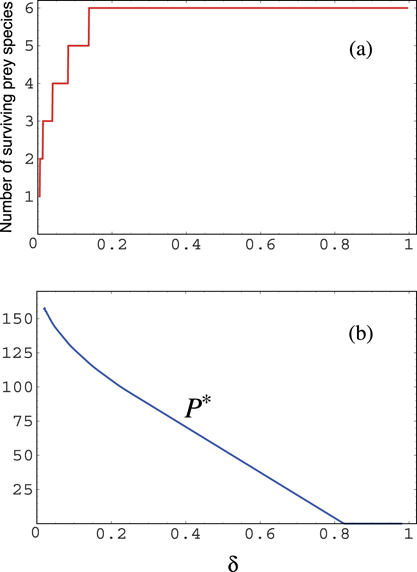
Figure 1. A numerical result about the δ-dependence of the equilibrium state for (1) after a shared predator's invasion into the system with coexisting six prey species. (a) Number of surviving prey species; (b) Equilibrium size of the predator population. ci = 0.1; r1 = 0.1; r2 = 0.115; r3 = 0.13; r4 = 0.145; r5 = 0.16; r6 = 0.175; bi = 0.001; βi = 0.0001 (1 ⩽ i ⩽ 6).
Download figure:
Standard image High-resolution imageTheorem 2. The equilibrium state with the predator's extinction for the system (1),

is globally asymptotically stable if and only if

Since Rn can be regarded as monotonically increasing in terms of n from its definition, this theorem implies that the predator can survive only when a sufficiently large number of prey species are available. On the contrary, if we reduce the number of prey species available for a shared predator, the predator could go extinct. Moreover, it is implied that such an extinction of predator is most likely to be caused by the deletion of the prey species which has the largest value of cibiri/βi since the deletion of such a prey species reduces the value of Rn by the largest amount. So such a prey species could be regarded as a sort of 'keystone species' which is the most relevant for the shared predator's survival.
From theorem 2, we have the following corollary:
Corollary 1. If and only if δ < Rn, the predator of (1) can survive.
When the predator survives, some prey species could go extinct because of the apparent competition effect. In the following arguments, we will focus on the feature of the system (1) with respect to which prey species can coexist with the surviving shared predator.
Let us consider now the following type of an equilibrium state  for (1):

with ![${H}_{\left[k\right],i}^{{\ast}}{ >}0$](https://content.cld.iop.org/journals/1751-8121/53/41/415601/revision2/aabadb8ieqn2.gif) (i = 1, 2, ..., k) and
(i = 1, 2, ..., k) and ![${P}_{\left[k\right]}^{{\ast}}{ >}0$](https://content.cld.iop.org/journals/1751-8121/53/41/415601/revision2/aabadb8ieqn3.gif) . From (1), this equilibrium state
. From (1), this equilibrium state  can be uniquely given by

where

From (7), we can find the following condition for the existence of the equilibrium  :
:

From (3), since ri+1/bi+1 ⩽ ri/bi (i = 1, 2, ..., n − 1), the condition (9) is equivalent to the following:

For the convenience of the mathematical arguments in the following part, we show here the following lemma:
Lemma 1. The sequence {Rk − (rk/bk)Bk} (k = 1, 2, ..., n) is non-negative and non-decreasing.
Indeed, from (3) and (8), we have
and R1 − (r1/b1)B1 = 0 necessarily from the definition (8), which shows the non-decrease and the non-negativity of the sequence at the same time.
Now we define a specific index of prey species  by
by

From the definitions (7) and (8), since

it is necessarily satisfied that  . Then we note that

because of lemma 1.
We can prove the following two theorems with respect to the existence and the stability of the equilibrium state  (appendix
Theorem 3. The equilibrium state  with
with  exists and it is globally asymptotically stable if and only if

Theorem 4. The equilibrium state  exists and it is globally asymptotically stable if and only if

The state  is the equilibrium with all prey species and the shared predator coexisting. The global stability can be proved by making use of the Lyapunov function. Especially for the equilibrium state
  with the surviving predator and only prey 1, we can get the following corollary from theorem 3:
Corollary 2. The equilibrium state  exists and it is globally asymptotically stable if and only if

This is actually because R1 − (r1/b1)B1 = 0 in (13) necessarily from the definition (8).
Finally, the conditions for the existence and the global stability of equilibrium states given by (5), (13)–(15) are complementary so that the union of those conditions for all equilibria covers all parameter region from lemma 1. As a consequence, we have arrived at the result consistent with theorem 1, clarifying the condition about which equilibrium state becomes globally asymptotically stable.
Since these theorems have shown that the reachable equilibrium state is (4) with the predator's extinction or  defined by (6), we can have the following result:
Corollary 3. For the system (1), any equilibrium with the surviving predator other than the type of  defined by (6) is always unstable even if it exists.
For example, it is possible to consider an equilibrium state such that Hi = 0 (i < k), Hj > 0 (j ⩾ k), and P > 0 for a number k > 1. Our result shows that such an equilibrium state is unstable even if it exists. This result is based on our numbering of the prey species by (3).
4. Deletion of a prey species
For the system (1), we consider the state transition after the deletion of a prey species from a globally asymptotically stable equilibrium state with the shared predator and its preys (more than one) coexisting. In this paper, the 'extinction' means a consequence of the internal population dynamics between prey and predator, whereas the 'deletion' may be caused by the other kinetics, for example, by a human activity or by a stochastic ecological disturbance. In a more mathematical sense, the 'deletion' of a prey species results in the reduction of the dimension of our system from n + 1 to n, while the 'extinction' must be necessarily considered for the system (1) of n + 1-dimension.
We can obtain the following theorem (appendix
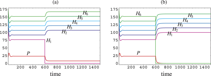
Figure 2. Temporal variation of population sizes after the deletion of a prey species at t = 600 from the coexistent equilibrium state with a shared predator and six prey species. (a) Prey H1 is deleted. No secondary extinction occurs; (b) Prey H6 is deleted. The shared predator goes extinct after the deletion. P(0) = 20.0; H1(0) = 100.0; H2(0) = 115.0; H3(0) = 130.0; H4(0) = 145.0; H5(0) = 160.0; H6(0) = 175.0; δ = 0.48; ci = 0.7; r1 = 0.1; r2 = 0.115; r3 = 0.130; r4 = 0.145; r5 = 0.16; r6 = 0.175; bi = 0.001; βi = 0.001 (1 ⩽ i ⩽ 6).
Download figure:
Standard image High-resolution imageTheorem 5. If a prey species is deleted from the coexistent equilibrium state, the system alternatively transfers to the state at which the predator coexists with the rest of prey species or the state at which the predator goes extinct.
This theorem indicates that the deletion of a native prey species from the coexistent equilibrium state does not cause any secondary extinction of any other native prey species due to the effect of apparent competition.
Further, we can obtain the following result about the predator population size at the equilibrium state transferred from the coexistent equilibrium state by the deletion of a prey species (appendix
Theorem 6. By the deletion of a prey species from the coexistent equilibrium state, the system transfers to an equilibrium state at which the predator population necessarily has a size smaller than before. Simultaneously each of the surviving prey populations at the new equilibrium state has a size greater than before.
The last part of the above theorem can be easily seen from (7). A numerical example is given in figure 2.
5. Introduction of a prey species
In this section, we consider the state transition from the coexistent equilibrium state with a shared predator and its native preys by the introduction of an alien prey species. From theorems obtained in the previous sections, the system transfers to one of the following four states after the introduction of an alien prey species (see figure 3):
- The introduced alien prey goes extinct, and the system returns to the original state.
- The system transfers to the coexistent equilibrium state with the introduced alien prey species and all native species.
- Some native prey species go extinct, and the predator coexists with some surviving native and the introduced alien prey species.
- Every native prey species goes extinct, and the predator coexists with the introduced alien prey species.

Figure 3. Temporal variation of population sizes after the introduction of prey H3 at t = 600 into the coexistent equilibrium state with the shared predator and two prey species. (a) b3 = 0.000 85. No extinction occurs. (b) b3 = 0.000 77. Prey H2 goes extinct. (c) b3 = 0.0007. Prey H1 and H2 go extinct. Commonly, P(0) = 20.0; H1(0) = 300.0; H2(0) = 300.0; H3(600) = 1.0; δ = 0.3; c1 = c2 = 0.3; c3 = 1.2; r1 = 0.2; r2 = 0.19; r3 = 0.18; b1 = b2 = 0.001; β1 = β2 = β3 = 0.0001.
Download figure:
Standard image High-resolution imageWe can prove the following theorem (appendix
Theorem 7. If an alien prey species satisfying the conditions below is introduced into the coexistent equilibrium state  of (1), the system transfers to the equilibrium state with the predator, the introduced alien prey species, and the native n − k prey species from the 1st to the kth (<n), while the native prey species from the k + 1th to the nth go extinct.

where parameters c•, b•, β•, and r• are of the introduced alien prey species.
From theorem 7, we can find the following corollary:
Corollary 4. If an alien prey species satisfying the conditions below is introduced into the coexistent equilibrium state  of (1), the system transfers to the coexistent equilibrium state
  without the extinction of any species:

From the first condition of (17), the transition to the coexistent equilibrium state  with n + 1 prey species requires a sufficiently large value of r•/b•. We remark that the first condition is always satisfied if r•/b• ⩾ rn/bn, while the second is always satisfied if r•/b• < rn/bn. Furthermore, if r•/b• = rn/bn, the condition (17) is satisfied independently of the parameters. Thus, any alien prey species satisfying r•/b• = rn/bn can successfully invade in the considered coexistent equilibrium state.
Next we can find the following corollary for the case that the introduced alien prey species goes extinct:
Corollary 5. If an alien prey species satisfying the condition below is introduced into the coexistent equilibrium state  of (1), the introduced alien prey species goes extinct, and the system returns to the original state:
This result indicates that the extinction of the introduced alien prey species, that is, the failure of its invasion depends only on the parameters r• and b•, and not on the other parameters including the energy conversion rate c• for its predation, and its intraspecific density effect β•. Thus, the success of the introduction of an alien prey species is determined only by the ratio r•/b•, whereas the consequence arising after its successful introduction depends also on the other parameters of the introduced alien prey species.
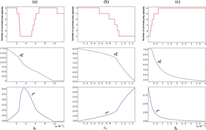
As shown in figure 4(a), if the introduced prey species is difficult enough to be preyed on (with sufficiently small b6), its introduction does not cause any extinction of the native species and the system transfers to the new coexistent equilibrium state with the introduced prey species. Such a new coexistent equilibrium state could be realized also when the introduced prey species is moderately easy to be preyed on, whereas the introduced prey species goes extinct if it is really easy to be preyed on. It is very interesting that, when the introduced prey species is moderately hard to be preyed on (for a certain intermediate range of the value of b6), the introduction of such an alien prey species causes the elimination of every native prey species and results in the equilibrium state with only the introduced alien prey species and the predator.
Figure 4. Parameter dependence of the equilibrium state after the introduction of a prey H6 into the system at the coexistent equilibrium state with a predator and five prey species. Numerical calculations on the number of surviving prey species, the equilibrium population size of the introduced prey H6, and that of the shared predator. (a) b6-dependence with (c6, β6) = (1.2, 0.0001); (b) c6-dependence with (b6, β6) = (0.0005, 0.0001); (c) β6-dependence with (c6, b6) = (0.7, 0.0008). Commonly, δ = 0.38; ci = 0.7 (1 ⩽ i ⩽ 5); r1 = 0.2; r2 = 0.195; r3 = 0.19; r4 = 0.185; r5 = 0.180; r6 = 0.175; bi = 0.001 (1 ⩽ i ⩽ 5); βi = 0.0001 (1 ⩽ i ⩽ 5).
Download figure:
Standard image High-resolution image
As shown in figure 4(b), if the predator's energy conversion rate for the introduced prey species is sufficiently small, its introduction does not cause any extinction of the native species and the system transfers to a new coexistent equilibrium state with the introduced prey species. In contrast, if the predator's energy conversion rate for the introduced prey species is large, the introduction of such an alien prey species causes the extinction of some native prey species due to the apparent competition effect. If the energy conversion rate is sufficiently large, the introduction of such an alien prey species eliminates every native prey species and results in the equilibrium state with only the introduced alien prey species and the predator.
As shown in figure 4(c), if the introduced prey species has a sufficiently strong intra-specific density effect, its introduction does not cause any extinction of the native species and results in the coexistent equilibrium state with the introduced prey species. If the introduced prey species has a weak intra-specific density effect, its introduction causes the extinction of some native prey species due to the apparent competition effect. Moreover, if the introduced prey species has a sufficiently weak intra-specific density effect, its introduction eliminates every native prey species and results in the equilibrium state with only the introduced prey species and the predator.
As for a specific case with ri/bi = ρ for any i, the introduction of any prey species with r•/b• = ρ in the coexistent equilibrium state of (1) always results in the transition to the coexistent equilibrium state with no extinction of any species, as shown by corollary 4. Hence, in such a case, any alien prey species with r•/b• = ρ can be successfully introduced into the native system without causing the extinction of any native species, so that the number of coexisting prey species is unbounded as long as the introduced prey species has the same value r•/b• as the native prey species, independently of the difference not only in the values of r• and b• themselves but also in any other parameter.
As for the predator population size at the equilibrium state transferred after the introduction of a prey species, with arguments similar to the proof of theorem 6 in appendix
Lemma 2. If the system transfers to a new equilibrium state without any extinction after the introduction of an alien prey species in the coexistent equilibrium state, the predator population at the new coexistent equilibrium state has a size greater than before.
Moreover, we can prove the following lemma, too (appendix
Lemma 3. If the system transfers to a new equilibrium state without the extinction of the introduced prey species and the predator, the predator population size is larger as the number of surviving prey species gets smaller at the new coexistent equilibrium state.
Consequently, we have the following theorem:
Theorem 8. The successful invasion of an alien prey species always results in the increase of the predator population size, independently of the number of surviving native prey species at the new equilibrium state. Moreover, as the number of extinct native prey species is larger, the predator population size at the new equilibrium state becomes greater than before the introduction of an alien prey species.
As the predator population size increases, each of surviving native prey populations at the new equilibrium state has a size smaller than before. This can be easily seen from (7).
6. Concluding remarks
In this paper, we analyzed the Lotka–Volterra n prey-1 predator system (1), focusing on the transition of the equilibrium state due to the deletion or the introduction of a prey species. As shown in theorem 3, we determined the necessary and sufficient condition for the predator's extinction (theorem 2), because a globally asymptotically stable equilibrium state always and uniquely exists for (1) from theorem 1.
Which preys could coexist with an shared predator? At the globally asymptotically stable equilibrium state, the extinct prey species has the smaller value of r/b in our model (theorem 3). The predator goes extinct if every available prey species has very small value of r/b (theorem 2). As a special case, if every prey species has a common value of r/b, the number of prey species with which the shared predator can coexist is unbounded for the Lotka–Volterra n prey-1 predator system (1), independently of the difference not only in the values of r and b themselves but also in any other parameter.
These results imply that for the stable existence of a food web with a generalist predator and a certain number of its preys, the value of r/b for its prey species would come to have a large average and necessarily small variance after a sequence of changes in the member of prey species following their extinction and invasion. This was mentioned also in [16, 20] as the high species diversity under the condition that the value of r/b is similar for all prey species. Furthermore this may be related to the 'biotic homogenization', the process making the species composition more similar after the alien species invasion, as Dangremond et al [9] discussed about the plant community with relation to the apparent competition.
Consequence of the deletion of a prey species. Deletion of a prey species from the equilibrium state with a shared predator does not cause the extinction of any other prey species, whereas the predator may go extinct (theorem 5). In case of no secondary extinction induced by the deletion of a prey species, each prey population size becomes larger than before while the predator population size becomes smaller (theorem 6). Hence this case can be regarded as a decrease in the number of prey species available for the predator to result in the reduction of the apparent competition effect on each prey species.
The deletion of a prey species which has the greater value of cb(r/β) is more likely to cause the predator's extinction (theorems 2 and 5). Such a prey species is easily preyed on and provides a high predator reproduction, or has a relatively large carrying capacity. In the context of a pest control, in order to suppress/eliminate the pest population regarded as a generalist predator, it would be a good option to identify such a prey species for the pest and reduce its population size.
Consequence of the introduction of alien prey species. Introduction of an alien prey species could strengthen the apparent competition effect on each prey species. In such a case, some native species would go extinct, while the system would transfer to the equilibrium state with the predator, the introduced prey species and some surviving native prey species (theorem 7). Hence, a series of the invasion of alien prey species could cause the decrease of the number of prey species available for the predator due to the extinction of native prey species by the apparent competition, and subsequently the system would come to have the predator species and only one prey species (see figure 3(c)). In such a case, the predator is identified as a specialist predator. From theorem 2 and corollary 1, as for the stable existence of such a specialist predator, the value of r/b characterizing the prey species would be large enough.
In contrast, the introduction of an alien prey species may result in no extinction of any species, and then the system transfers to the coexistent equilibrium state with the predator, all native prey species and the introduced alien prey species (theorem 7). In such a case, the equilibrium predator population size becomes larger than before, while the equilibrium prey population sizes get smaller (lemma 2). We could regard this case as an increase in the number of available prey species to cause the stronger apparent competition effect. Indeed Messelink et al [27] investigated the biological control by a generalist predator in a laboratory system of three pest species (western flower thrips, greenhouse whitefly, and spider mite) and their predator (predatory mite), in which such a dependence of the predator population size on the composition of prey species was clearly observed.
Predator population size at the equilibrium state. The predator population size becomes larger as the number of surviving prey species gets smaller due to their deletion and introduction. Then each of coexisting prey population sizes gets smaller (theorem 8). As the number of extinct prey species due to the successful introduction of alien prey species gets larger, the surviving prey species undergo stronger apparent competition effect. In such a case, the apparent competition effect from the introduced prey species would overcompensate that from those native prey species which have gone extinct. In short, the successful introduction of alien prey species which could cause a strong apparent competition effect is likely to result in the extinction of some native prey species. From the viewpoint of the predator, such extinction of some native prey species due to the introduction of alien prey species consequently appears as an exchange of some available prey species with the other species preferable for the predator's reproduction.
As a consequence, the introduction of alien prey species into the equilibrium state with a shared predator and its prey species never reduces the predator population size at the equilibrium state, and causes the stronger effect of apparent competition whenever the introduction of the alien prey species results in its successful settlement. In contrast, the deletion of a prey species from the equilibrium state with a shared predator and its prey species never causes any secondary extinction of the other prey species, and could cause only extinction of the predator. These results may be regarded as corresponding to those given by Petchey [33], who investigated some microcosms of bacteria and bacterivores in laboratory and showed that the prey diversity can affect the predator population dynamics. As implied by our theoretical arguments above, the apparent competition could be a significant factor to determine the structure of foodweb, tangled with the other interspecific reactions within it, as discussed in [12, 14, 32, 35, 36].
Implication for pest control. In the context of pest control, we suggest from our results that the introduction of alien prey species would be effective only if the purpose of the pest control is to reduce the population of a native prey species (which is the pest), while the deletion of a native prey species would be effective only if the purpose is to reduce the predator population (which is the pest).
For biological control in agroecosystems, the introduction of an alien species would be a better choice compared to the deletion of a native species. In grape vineyards, Karban et al [25] found that the release of economically unimportant Willamette mites alone, or of predatory mites alone fails to significantly reduce populations of the damaging Pacific spider mite. However, when both herbivorous Willamette and predatory mites were released together, the population of the Pacific mites was reduced. This may be regarded as a case when the introduction of an alien prey species (the herbivorous Willamette mite) would be effective to reduce a native prey population (the Pacific mite) if there is a shared predator (the predatory mite). As Holt and Hochberg [19] discussed, the indirect interactions may contribute to the biological control in such a way. At the same time, it should be kept in mind that the introduction of an alien species as a biological control agent would cause the decrease of some native species populations other than that of the target pest species [5].
In the context of spatial heterogeneity. As Holt [17] highlighted, our n prey-1 predator system with no direct interspecific reaction between prey species can be translated in the context of spatial heterogeneity as a system with a spatially heterogeneous environment composed of n patches for the habitat of a prey species. Assuming that the prey mobility between patchy habitats is negligible or impossible, and that the predator mobility has the spatial scale large enough to cover the area of all patches, the prey subpopulations of those patches undergo the effect of apparent competition through the predator population. The prey's population dynamics is affected by the environment at each patch, so that its nature would be different from patch to patch.
In such a setup, the result for the Lotka–Volterra n prey-1 predator system (1) implies that the apparent competition could cause the extinction of prey population at some patches, that is, a sort of local extinction of a prey species. The deletion of a prey species in this paper could be translated into the destruction of a patch, while the invasion of an alien prey could be mean the appearance of an additional patchy habitat of the prey species by a human operation or by a certain change of predator's spatial distribution.
Although our results are from a simple mathematical model, we believe that they could demonstrate that apparent competition effect could drive some species to extinction. This finding could be useful for pest control. In contrast to lots of previous theoretical works related to apparent competition which discussed the effect of predation on the diversity of competing prey species, we considered only how apparent competition affects the coexistence of a shared predator and its prey species. We expect that our mathematical work will be helpful for some future theoretical works on this problem and some other related ones.
In this paper, we considered the simplest Lotka–Volterra prey-predator system with the mass-action term which introduces the predation effect between prey and predator. The modification with the introduction of such an intraspecific competition effect within the predator population, for instance − P2, may not change the essence of our results. This could be shown by mathematical analyses similar to ours. However, for some other types of prey-predator system with different terms for predation, stable periodic solution or bistability state can appear as evident in models with switching predation (for example, see [28, 39]). As implied by Noy-Meir [31], even the simple mathematical model of prey-predator population dynamics may show a specific behavior, depending on the assumptions for the dynamical nature of the interaction between prey and predator. Further this kind of theoretical/mathematical work is closely related to the theory of community assembly which we did not consider deeply here (readers interested in the theory can see relevant literature cited in this section and the references therein).
Acknowledgments
The authors greatly appreciate anonymous referees for their valuable comments on the first version of the manuscript, and Emmanuel J Dansu for his help about the manuscript revision. The author HS was supported in part by JSPS KAKENHI Grant No. 18K03407.
Appendix A.: Proof of theorem 2
At first, to prove theorem 2, we prove the following lemmas:
Lemma 4. If P(0) > 0, then P(t) > 0 at any time t > 0.
Lemma 5. If 0 < Hi(0) ⩽ ri/βi and P(0) > 0, then 0 < Hi(t) < ri/βi at any time t > 0.
Proof. Since there exists the solution such that P(t) ≡ 0 for any t for (1) with P(0) = 0. On the other hand, from (1), we can get the following formal equation:


The formal solution (A.2) for P(t) shows that P(t) > 0 for any t > 0, because of the uniqueness of the solution for (1). This proves lemma 4.
There exists the solution such that Hi(t) ≡ 0 for any t and any i for (1) with Hi(0) = 0. Hence, from the uniqueness of the solution for (1), the formal solution (A.1) for Hi(t) shows that Hi(t) > 0 for any t > 0 with Hi(0) > 0. Then, for Hi(t) > 0 and P(t) > 0, we have

for any t > 0. Therefore, if 0 < Hi(0) ⩽ ri/βi (i = 1, 2, ..., n), it is impossible that Hi(t) ⩾ ri/βi for any t > 0. Consequently we have lemma 5. □
By these lemmas, we can find that
Then, if δ > Rn, from the comparison theorem, we can find that

for any t > 0. From lemma 4, we find from (A.4) that P(t) → 0 as t → ∞ if −δ + Rn < 0.
Next, suppose that P(t) → 0 as t → ∞. From (1), we can easily see that Hi(t) → ri/βi (i = 1, 2, ..., n) as P(t) → 0. On the other hand, it is clear that the following equilibrium with P = 0 is always unstable for any k > 0:

because any prey population grows in a logistic manner without any predator. Thus, if P(t) → 0, the system (1) asymptotically goes to the equilibrium state (r1/β1, r2/β2, ..., rn/βn, 0). By the local stability analysis for the equilibrium state (r1/β1, r2/β2, ..., rn/βn, 0), we can easily prove that if P(t) → 0 as t → ∞, it is necessary that −δ + Rn < 0.
If δ = Rn, we have
for any time t > 0 by lemma 5. Therefore, P(t) → 0 as t → 0 again. These arguments prove theorem 2.
Appendix B.: Proof of theorems 3 and 4
Proof. First, we consider the existence of the equilibrium state  . When
  , from (11) and (12), we have (13). On the other hand, from the definition (8), we can easily find that

for k = 1, 2, ..., n. Therefore, from (12), we now have

Hence, when the condition (13) is satisfied, the condition (10) for the existence of the equilibrium  with
with  holds. So, the equilibrium state
  with
with  exists if the condition (13) is satisfied. When
  , the condition (14) is the condition (10) with
  for the existence of the equilibrium
  . This means that the equilibrium state
  exists if the condition (14) is satisfied with
  .
.
Next, let us turn to consider the stability of equilibrium state  . For the case of
  , we define the function

Then, from (1), the derivative of  becomes

where we especially used the following equations about the equilibrium state  :
:
From the definition of  by (11),

for any  and any t > 0, because of (3) and lemma 5 in appendix A. Thus, from (B.4) and (B.5), we have found that
  for any t > 0.
It can be easily found from (B.3) and (B.4) that  and
and  are zero only at the equilibrium
  , and further that
  is positive definite for any (H1, H2, ..., Hn, P) other than
  in
in  . This means that the function
  is the Lyapunov function for the equilibrium state
  , and we can conclude that
  is globally asymptotically stable in Ω. Taking account of corollary 2, this result with the above arguments about the existence of
  shows that the equilibrium state
  with
with  exists globally asymptotically stable for (1) if the condition (13) is satisfied. Consequently these arguments prove theorem 3.
For the case of  , let us consider the function

From (1), we can get the following derivative of Vn(t):
where dVn/ dt = 0 only when ![${H}_{i}\left(t\right)={H}_{\left[n\right],i}^{{\ast}}$](https://content.cld.iop.org/journals/1751-8121/53/41/415601/revision2/aabadb8ieqn53.gif) for every i, while Hi(t) cannot remain the value
for every i, while Hi(t) cannot remain the value ![${H}_{\left[n\right],i}^{{\ast}}$](https://content.cld.iop.org/journals/1751-8121/53/41/415601/revision2/aabadb8ieqn54.gif) besides being at the equilibrium state
besides being at the equilibrium state  . Since Hi(t) temporally varies as long as
 ![$P\left(t\right)\ne {P}_{\left[n\right]}^{{\ast}}$](https://content.cld.iop.org/journals/1751-8121/53/41/415601/revision2/aabadb8ieqn56.gif) even when
even when ![${H}_{i}\left(t\right)={H}_{\left[n\right],i}^{{\ast}}$](https://content.cld.iop.org/journals/1751-8121/53/41/415601/revision2/aabadb8ieqn57.gif) for every i, we can see that Vn(t) is monotonically decreasing in terms of t > 0, even though dVn/dt = 0 at some moments when
for every i, we can see that Vn(t) is monotonically decreasing in terms of t > 0, even though dVn/dt = 0 at some moments when ![${H}_{i}\left(t\right)={H}_{\left[n\right],i}^{{\ast}}$](https://content.cld.iop.org/journals/1751-8121/53/41/415601/revision2/aabadb8ieqn58.gif) for every i. Moreover, as long as P(t) > 0 and Hi(t) > 0, we have Vn ⩾ 0, where Vn = 0 only at the equilibrium state
for every i. Moreover, as long as P(t) > 0 and Hi(t) > 0, we have Vn ⩾ 0, where Vn = 0 only at the equilibrium state  . With the arguments same as above, Vn is the Lyapunov function for the equilibrium state
  . Therefore the equilibrium state
  is globally asymptotically stable if the condition (13) is satisfied with
  . Consequently these arguments prove theorem 4. For the further mathematical information about the analysis on the global stability with Lyapunov function, refer, for example, [13, 38] and the references therein. □
Appendix C.: Proof of theorem 5
Proof. By the similar argument about the condition (9) for  , the condition for the existence of the coexistent equilibrium state of the system with n − 1 preys after the deletion of prey k from the coexistent equilibrium state
  is given by

where

From theorem 2, the necessary and sufficient condition for the predator's extinction after the deletion of prey k is that δ > Rn\k.
In case of δ < Rn\k, substituting (14) with (C.2), we can rewrite the condition (14) for the coexistent equilibrium state  as follows:
From this condition, we have the following inequality:
Therefore, the following condition is necessarily satisfied:

This is equivalent to (C.1). Hence, from theorem 3, the coexistent equilibrium state of the predator and the remaining n − 1 prey species is globally asymptotically stable. These arguments prove theorem 5. □
Appendix D.: Proof of theorem 6
Proof. If the predator goes extinct after the deletion of a prey species at the coexistent equilibrium state  of (1), then the theorem holds. So, from theorem 5, we hereafter focus on the case when the system transfers to the equilibrium state with the predator and the remained prey species after the deletion of a prey species.
From (7), the predator population size ![${P}_{\left[n\right]}^{{\ast}}$](https://content.cld.iop.org/journals/1751-8121/53/41/415601/revision2/aabadb8ieqn67.gif) at the coexistent equilibrium state
at the coexistent equilibrium state  and the size
 ![${P}_{\left[n{\backslash}k\right]}^{{\ast}}$](https://content.cld.iop.org/journals/1751-8121/53/41/415601/revision2/aabadb8ieqn69.gif) at the equilibrium state approached after the deletion of prey k are respectively given by
at the equilibrium state approached after the deletion of prey k are respectively given by
where Rn\k and Bn\k are defined by (C.2). Now from the definition of Rn and Bn by (8), we can easily get the following equation:

Now from (14), we have δ > Rn − (rn/bn)Bn. Hence, from the condition that rk/bk ⩾ rn/bn by (3), we have δ > Rn − (rk/bk)Bn, and thus find that the right side of (D.1) is positive. As a result, ![${P}_{\left[n\right]}^{{\ast}}{ >}{P}_{\left[n{\backslash}k\right]}^{{\ast}}$](https://content.cld.iop.org/journals/1751-8121/53/41/415601/revision2/aabadb8ieqn70.gif) for any k (1 ⩽ k ⩽ n). □
for any k (1 ⩽ k ⩽ n). □
Appendix E.: Proof of theorem 7
Proof. Let us consider the introduction of a prey species with its parameters c•, b•, β•, and r•. We now define the following Rn⊕1 and Bn⊕1:

It is satisfied that Rn⊕1 > δ, since Rn⊕1 > Rn and Rn > δ on the condition of the globally asymptotically stable equilibrium state  . From theorem 4, n + 1 prey species can coexist with the shared predator after the introduction of the prey species if the following condition is satisfied:

On the other hand, since
it is possible that the condition (E.2) is not satisfied after the introduction of an alien prey species on the condition of the globally asymptotically stable equilibrium state  . If (E.2) is not satisfied, then from theorem 3, some native prey species go extinct while the system transfers to an equilibrium state with the predator, some surviving native prey species, and the introduced alien prey species. From theorem 3, if only k (<n) native prey species survive at the new equilibrium state with the predator and the introduced alien prey species, the stability condition (13) indicates that the following condition is satisfied:

In this case, we necessarily have r•/b• > rk+1/bk+1. Since δ > Rn − (rn/bn)Bn on the condition of the globally asymptotically stable equilibrium state  , we can find the following inequality:

If rk/bk ⩾ r•/b•, the first inequality of (E.3) becomes
which is satisfied because of (E.4). If r•/b• > rk/bk, the first inequality of (E.3) becomes

which can be rewritten as the first inequality of (16) in theorem 7, making use of (E.1).
Consequently we note that the first inequality of (16) in theorem 7 holds whenever rk/bk ⩾ r•/b•. Thus, the first inequality of (16) in theorem 7 is necessary and sufficient in order that the first inequality of (E.3) is satisfied. In the same way, the second inequality of (E.3) can be rewritten as the second inequality of (16) in theorem 7, making use of (E.1).
Lastly, if an alien prey species which satisfies (16) in theorem 7 is introduced into the coexistent equilibrium state  any prey species which has ri/bi less than rk/bk goes extinct, and the system transfers to the equilibrium state with the predator, k native prey species, and the introduced alien prey species. □
Appendix F.: Proof of lemma 3
Proof. Let us consider an introduced prey species characterized by parameters c•, b•, β•, and r•. From theorem 3, if the system transfers to the equilibrium state with the predator and k prey species (k < n) including the alien prey species, the condition that r•/b• > rk/bk must be satisfied, and then the predator population size ![${P}_{\left[\left(k-1\right)\oplus 1\right]}^{{\ast}}$](https://content.cld.iop.org/journals/1751-8121/53/41/415601/revision2/aabadb8ieqn75.gif) at the new equilibrium state must satisfy the following condition:
at the new equilibrium state must satisfy the following condition:

by the definition (11) of  .
.
In another case that an alien prey species characterized by parameters c•', b•', β•', and r•' is introduced into the coexistent equilibrium state  , if the system transfers to the equilibrium state with the predator and k' (>k) prey species including the alien prey species, the following condition must be satisfied:

Since rk'−1/bk'−1 ⩽ rk/bk for k' > k, we find from (F.1) and (F.2) that

Therefore, ![${P}_{\left[\left({k}^{\prime }-1\right)\oplus 1\right]}^{{\ast}}{< }{P}_{\left[\left(k-1\right)\oplus 1\right]}^{{\ast}}$](https://content.cld.iop.org/journals/1751-8121/53/41/415601/revision2/aabadb8ieqn78.gif) if k' > k. As for the other two cases that no extinction occurs and that only one native prey species goes extinct, we can show that
if k' > k. As for the other two cases that no extinction occurs and that only one native prey species goes extinct, we can show that ![${P}_{\left[n\oplus 1\right]}^{{\ast}}{< }{P}_{\left[\left(n-1\right)\oplus 1\right]}^{{\ast}}$](https://content.cld.iop.org/journals/1751-8121/53/41/415601/revision2/aabadb8ieqn79.gif) with the same arguments. □
with the same arguments. □