Intervention Scenarios to Enhance Knowledge Transfer in a Network of Firms
 Frank Schweitzer
 Yan Zhang
 Giona Casiraghi
- Chair of Systems Design, ETH Zurich, Zurich, Switzerland
We investigate a multi-agent model of firms in a Research & Development (R&D) network. Each firm is characterized by its knowledge stock xi(t), which follows a non-linear dynamics. xi(t) grows with the input from other firms, i.e., by knowledge transfer, and decays otherwise. However, maintaining the interactions that increase knowledge stock is costly for all partners involved. Because of this, firms leave the network whenever their expected knowledge growth is not realized. This, in turn, may cause other firms also to leave the network. The paper discusses two bottom-up intervention scenarios to prevent, reduce, or delay such cascades of firms leaving. The first one is based on the formalism of network controllability, in which driver nodes are identified and subsequently incentivized, by reducing their costs. The second one combines node interventions and network interventions. It proposes the controlled removal of a single firm and the random replacement of firms leaving. This allows to generate small cascades, which prevents the occurrence of large cascades. We find that both approaches successfully mitigate cascades and thus improve the resilience of the R&D network.
1. Introduction
Interventions belong to the tool box of systems design [1]. The ability to influence systems such that they reach a desired state or show a desired behavior, is not only of relevance for engineers and operators. This ability is also favored by managers or politicians, who wish to steer the dynamics of socio-economic systems toward a particular outcome. Most of the interventions in economic systems are targeted at the macro level, for instance by adjusting tax rates or legal conditions. They follow a top-down approach: a centralized decision to change some “boundary conditions” induces an adaptation of the system, hopefully in the right, i.e., wanted, direction.
This approach is contrasted with the bottom-up approach that targets system elements rather than systems as a whole [2–4]. It plays a major role in complex systems comprising a large number of elements, denoted as agents in the following. Bottom-up interventions can be targeted either at specific agents or at their interactions or at the network as a whole [5]. In socio-economic systems, agent specific interventions include, for example, monetary incentives (e.g., reduced costs, bonuses) or privileged access to resources (e.g., information, credit) [6, 7].
Complex socio-economic systems are often represented as networks, where agents are depicted as nodes and their interactions as links. To utilize a bottom-up approach of interventions requires to solve a number of problems that are later addressed also in this paper. First of all, we need to find out which agents are the most promising ones to drive a system, i.e., we need to identify driver nodes. This problem can be only tackled if we know how agents influence another, i.e., we need to specify the dynamics on the network. Secondly, we need to determine the desired state of the system, and eventually we need to calculate the appropriate intervention that is suitable to drive the network toward this state.
These problems are exacerbated if, in addition to the dynamics on the network, there is also a dynamics of the network. That means, the network itself changes because (i) agents join or leave the network or (ii) add, remove, or rewire their links to other agents. The dynamics of the system is then described by two time scales, one at which interactions happen, and one at which the network evolves, e.g., at which different agents enter or leave the network. Most real-world socio-economic systems are characterized by these couplings of time scales. For example, online social networks become quite volatile because users enter and exit and also change their interactions with other users at high frequency. This makes it difficult to assess the robustness of such systems. If users start to leave and this way generate large cascades of other users leaving, these networks may even collapse [8].
To model the direct and indirect impact of nodes leaving a network, two different approaches are followed. The first one focuses on the network topology, specifically on the degree of the nodes and their embedding. One example is the k-core decomposition model [9, 10] to explain cascades. The second one also includes the internal dynamics of the nodes, for example the threshold model [11, 12]. Combinations of these approaches, such as the KQ model [13] lead to a better formal understanding of the emergence of systemic risk [14–16], i.e., the collapse of a large part of the system because of failure cascades.
Also economic networks are prone to failure cascades and decline [17, 18]. In this paper, we discuss the case of R&D networks, used for the knowledge exchange between firms. Empirical studies have shown that such networks exhibit a life cycle dynamics, i.e., they grow and later decay [19, 20] because in R&D collaborations firms usually terminate their interactions after some time. Either the purpose of their collaborations is fulfilled, e.g., a number of patents are filed, or it is not fulfilled. For example, firms have not obtained an expected knowledge stock or an expected growth of knowledge and therefore decide to leave the network to save the costs involved in collaborations. If firms leave, this may cause other firms to leave as well, because they lost the input from their collaboration partners. Thus, before we can think of interventions, we need to model this process, which is provided in section 2.
Based on these insights, we will then develop two different approaches toward interventions in sections 3, 4. The aim of these interventions is to prevent large cascades of firms leaving the collaboration network. If that is not entirely possible, we want at least to reduce the size of such cascades, or to delay them. Our first approach is rooted in control theory [21, 22] applied to complex networks, a recent development that lead to the concept of network controllability [23]. Basically, we identify a set of driver nodes with two different methods, to which an incentive is applied. The formal method relies on a linear dynamics on the network, which is often not given. Generalizations to non-liner problems are not straightforward, as discussed in [24, 25]. For these reasons, we will mainly use computational methods in this paper.
To contrast the formal approach, our second approach is based on heuristics, that means on experience and intuition. It combines two different types of interventions: a network intervention, targeted at the whole network to allow a continuous evolution, and a node intervention targeted at only one firm. It was already shown, for the simpler case of a linear dynamics, that such heuristic approaches can significantly improve the robustness of networked systems [26]. Here we investigate the case of a non-linear dynamics and a fixed driver node. We are mainly interested to see how this heuristic intervention fares in comparison to the formal intervention based on network controllability. What are the advantages and shortcomings of these two different interventions? And to what extent can they be applied to a knowledge exchange network of firms? These questions will be discussed in section 5.
2. Generation of Knowledge Stock
2.1. A Network Model of Interacting Firms
2.1.1. Knowledge Stock
In the following, we utilize a multi-agent model of firms i = 1, …, N, which are each characterized by a scalar variable xi(t), their knowledge stock. This summarizes for example the R&D (research and development) experience of a firm, measurable by its number of patents and research alliances. xi can have continuous values which have to be positive, and can change over time at a time scale t.
To specify this dynamics we first note that the value of the knowledge stock continuously decreases if it is not maintained. Hence, we consider a decay term −γxi(t) with a decay rate γ characterizing the life time of the knowledge stock. To compensate for the decay, we need to make assumptions about the growth of the knowledge stock. One could reasonably argue about a source term that reflects inhouse R&D activities [27]. The main focus in our paper, however, is on knowledge transfer. Therefore, we assume that the growth of xi is mainly driven by input from other firms, i.e., by R&D collaborations, rather than by own research activities. This reflects empirical observations for innovation networks of firms [19].
2.1.2. Network Representation
To model knowledge transfer, we use a network, in which nodes represent agents, i.e., firms, and links their interactions. The network approach implies that interactions in a group of N firms, e.g., in R&D alliances between 2 and 10 firms, are decomposed into dyadic interactions between any two of these N firms. We further consider direct interactions between firms. That is, an interaction i → j describes that firm i transfers knowledge to firm j, but this does not necessarily has to be reciprocal, i.e., j ↛ i is possible. With N firms, there are N(N − 1) different directed dyadic interactions possible. Whether they take place is described in an adjacency matrix A of size N × N, in which an entry aij = 1 indicates a link i → j, and aij = 0 its absence. Empirical investigations have shown that such matrices for R&D collaborations are usually sparse, that means the number of links is of the order N rather than N2. Based on the entries in the adjacency matrix we can define the in-degree of a firm i as the number of incoming links from other firms, and the out-degree as the number of outgoing links to other firms. Note that in general aij ≠ aji.
2.1.3. Knowledge Growth
Our main assumption is that the knowledge growth of firm i is determined by the knowledge stock of those firms j that have direct link to i, as expressed by the aji, i.e., it is proportional to xj(t), with the proportionality constant b to weight the benefit. Further, it is reasonable to consider a saturation for the growth of knowledge stock. At higher levels of xi, it becomes more difficult for firm i to “absorb” new knowledge, i.e., to incorporate it into a firm because of the internal complexity associated with the way knowledge is stored and linked internally. This absorptive capacity is for simplicity reflected in a quadratic term , as known from saturated growth dynamics [28].
The proportionality factor ĉ for the saturation effect, however, deserves a discussion, as there are different arguments possible. It could be simply a constant, ĉ ≡ c0, to reflect that the saturation effect depends mainly on the knowledge stock of firm i. On the other hand, it could be also an individual variable, ĉ ≡ ci, to incorporate further influences. One possibility is a dependency on the in-degree, , based on the argument that a larger number of firms transferring knowledge to firm i makes the absorption of knowledge more difficult. Another possibility is a dependency on the out-degree, , based on the argument that, in addition to the absorption of knowledge, firm i also has to maintain links to other firms j, which consumes resources, and therefore exacerbates the problem. In this paper, we follow the latter argumentation which was also used in [29], i.e., .
Combining these assumptions, we propose the following dynamics for the knowledge stock [29]:
Here, it is additionally considered that some links, denoted by pji, provide firm i with a direct input from particular valuable firms. For example, instead of obtaining indirect knowledge input from a firm k via other firms j, firm i would much more benefit if k had a direct link to i. So, if pji = 1, there will be an extra benefit bext from interacting with this valuable agent. Such shortcut externalities have been discussed [e.g., [29, p. 247]]. In the following, we drop this term in the dynamics, to simplify the analysis.
2.1.4. Direct and Indirect Reciprocity
The above dynamics leads to a stationary, but non zero value of the knowledge stock only if the network contains cycles of firms benefiting another, as illustrated in Figure 1. The shortest possible cycle involves two firms, for example 1 → 2, 2 → 1 in Figures 1A,B. This mutual interaction relates to direct reciprocity, as firm 1 contributes to the knowledge stock of firm 2 and the other way round. But these cycles can be also larger, as Figure 1C illustrates. In this case, firm 1 still contributes to the knowledge stock of firm 2, but does not receive a reciprocal benefit from firm 2. Still, firm 1 benefits from being part of a closed cycle 1 → 2 → 4 → 5 → 1, i.e., it receives an indirect benefit from firm 2, via firms 4 and 5. Such constellations relate to indirect reciprocity, which plays an important role also in the emergence of cooperation [30]. Also the development of technology depends on the existence of such feedback cycles [31]. Hence, links that contribute to closing these cycles in the interaction network could for example receive an extra benefit, bext, although this is not considered here.
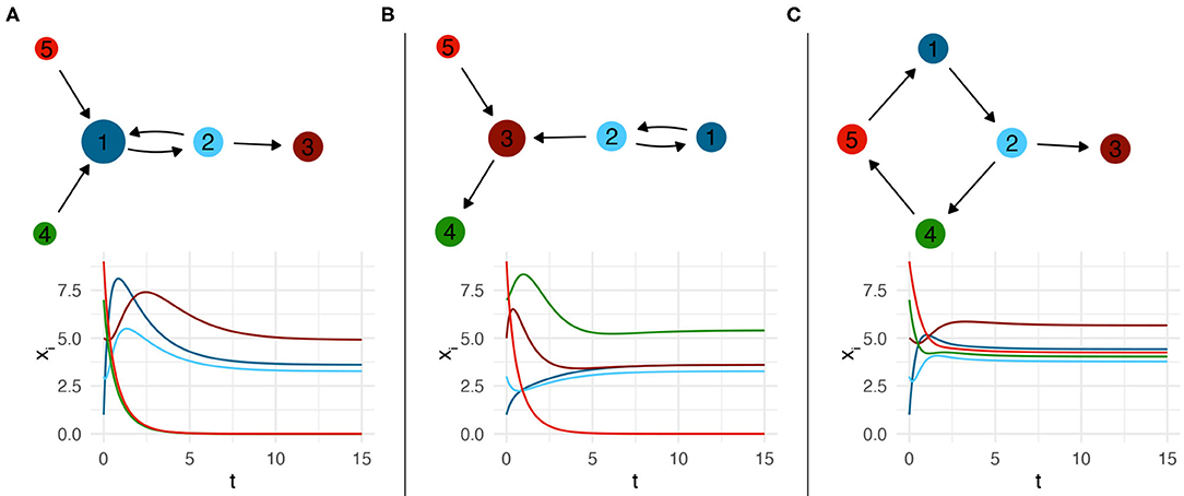
Figure 1. Dynamics of the knowledge stock, Equation (1), in a small network of 5 firms. The size of a node is proportional to its in-degree. The color of the each knowledge stock's line matches that of the corresponding node in the respective network. (A–C) show the dynamics for three different network configurations.
It is worth noticing that not all firms need to be part of cycles, to obtain a non-zero knowledge stock. In Figure 1A, we show a configuration where firm 3 benefits from the knowledge transfer from firm 2, but does not contribute in a reciprocal manner. Because this even saves the costs from maintaining the links, firm 3 obtains the highest value x3. Comparing Figures 1A,B, we see that firm 3, even with a higher in-degree, does not necessarily have the highest value x3. This points to the impact of the non-linear dynamics of the knowledge stock, which cannot be simply reduced to the influence of in-degrees.
Eventually, we note that firms reach a non-trivial stationary knowledge stock only if they are connected to a cycle. In Figure 1A, Firms 4 and 5 contribute to the knowledge stock of firm 1, but do not receive any reciprocal contribution. Hence, x4 → 0 and x5 → 0 over time.
In general, the existence of non-trivial steady states, i.e., xi(t → ∞) > 0, for firms i that are part of a network , , can be ascertained by studying the irreducibility of the graph [29, 32]. In particular, the existence of at least one closed cycle in the graph is sufficient to assure that both firms in the cycle and firms that receive links from firms within the cycle have a non-zero stationary knowledge stock. Moreover, for special classes of graphs it is possible to find analytical solutions for the values of the steady states [29].
2.2. Decision to Leave the Network
2.2.1. Knowledge Stock and Growth
Firms participate in knowledge transfer because they have the expectation that their knowledge stock grows over time. So, it is reasonable to assume that after the knowledge stock dynamics has converged to the stationary value, they evaluate the performance. Based on this, they may decide to leave the network, i.e., to cut all their outgoing links. Because this decision is based on the stationary values of the knowledge stocks, , it takes place at a different time scale T, which is longer than the time scale t at which the knowledge stock reaches its stationary value.
Specifically, we consider that at each time step T, firms compare (A) their absolute value of the knowledge stock, with a threshold, xthr (equal to all firms), and (B) their growth of the knowledge stock in the past time step, with a threshold, gthr (equal to all firms). They decide to continue to collaborate only if both of their respective values are above the thresholds. If any of these two conditions are not met, firms decide to leave with a certain probability p, which implies that they do not immediately leave.
We note that both conditions reflect different aspects that influence firms decisions. Condition (A) uses a cost/benefit assessment. If, in the current situation, the costs are higher than the benefits from receiving knowledge input, firms may choose to leave. That means, higher values of xthr consider a sensitivity for higher costs. Condition (B), on the other hand, captures to what extent the expectations of firms regarding the growth of knowledge stock are met. Higher values of gthr therefore indicate a lower tolerance of firms, if their expectations are not met.
If firms leave the network, this impacts the transfer of knowledge between firms in two ways: (i) directly, because firms leaving no longer contribute to the knowledge stock of their previous partners, (ii) indirectly, because firms leaving change the structure of the network and this way also the cycles of indirect reciprocity. This, on the other hand, generates an impact on the knowledge growth and the knowledge transfer of the remaining firms in the next time step. Hence, at time T + 1 the remaining firms obtain a different knowledge stock, xstat(T + 1) and a different growth rate, g(T + 1). This may cause other firms to leave the network, i.e., we observe cascades of firms dropping out. Such observations are in qualitative agreement with empirical studies about the life cycle of R&D network, where indeed a decline of firms participating can be found [19].
2.2.2. An Example
Figure 2 illustrates such a cascade of firms leaving the network. At time steps T = 1, 5, the firms colored in gray leave the network because their knowledge stocks fell below the threshold value xthr (condition A). At time steps T = 2, 3, 4, 6, on the other hand, the firms colored in gray leave the network because their expectations about their knowledge growth fell below the corresponding threshold gthr (condition B). These firms have indeed a high knowledge stock, i.e., they pass condition (A). That means, with just the comparison of knowledge stock, we would not observe that a cascade emerges. The comparison of knowledge growth thus adds a new element to the dynamics. Because expectations are considered, we observe in our model that also firms with a high knowledge stock and a high number of connections from partners may decide to leave the network, which makes our model different from other cascade models [11, 12, 16].
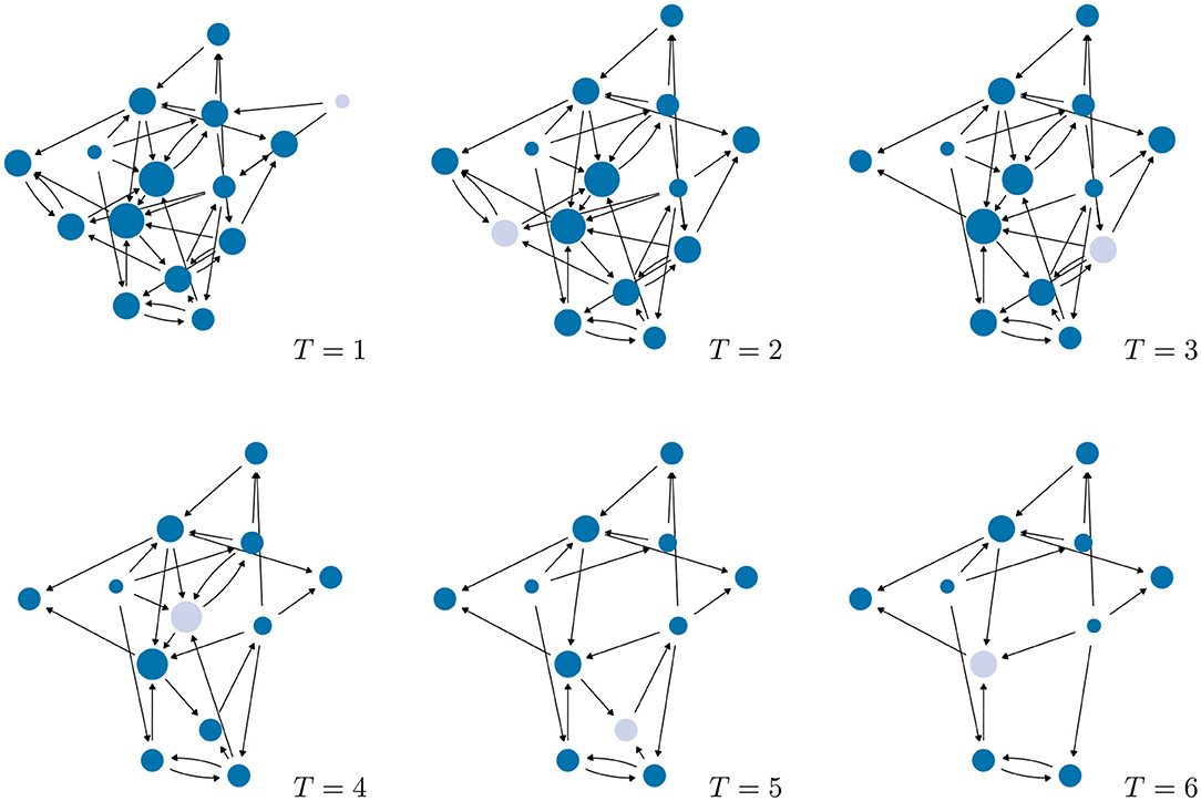
Figure 2. Cascades of firms leaving a sample network of N = 15 without any network intervention. The position of the nodes is fixed and their size proportional to their current in-degree. Firms colored in gray will leave the network in the next time step T. Parameters: γ = 0.5, b = 0.2, c = 0.06, xthr = 0.05, gthr = 0.8, p = 0.1.
3. A Formal Approach to Interventions
3.1. Interventions and Network Topology
The above discussion makes very clear that our interventions shall prevent the breakdown of the network of firms collaborating in knowledge exchange. As our ultimate aim, we want to (i) prevent cascades of firms leaving the network or, if that is not entirely possible, (ii) reduce the cascade size such that the majority of firms still remains in the network, or (iii) delay the occurrence of cascades such that the network remains at least for a given time horizon, .
This closely relates to investigations of systemic risk, which is measured by the fraction X(t) of failing agents/nodes in a system. Systemic risk usually emerges from the early failure of very few agents, which affects other agents and causes them to fail, this way leading to a failure cascade. If X(t) approaches 1, most parts of the system are destroyed. Therefore, we can quantify the aim of our intervention strategies as keeping low, precisely below 0.5. This means, the majority of firms stays in the network for a finite, but large time .
This aim can be achieved by interventions on the network level and/or the node level. In the following, we discuss two scenarios that combine interventions on these levels in different ways. In this section, we take a formal approach to network interventions that focuses on the node level, based on the formalism of network controllability. In section 4, instead, we describe a heuristic approach that smartly combines interventions at the node and network level to achieve our aim. We validate all our scenarios by means of computer simulations.
We start with addressing the node level. Here, the decisions of individual firms to leave is influenced via their knowledge stock (Equation 1). A trivial approach would be to simply lower the costs c of all firms, this way increasing their knowledge stock and forcing them to stay. Another trivial variant would be to reduce the probability p of firms to leave if their conditions (A) or (B) to stay in the network, are no longer met. We do not follow these trivial approaches which treat all firms equal. Instead, we want to make use of an important feature that distinguishes firms, their topological position in the collaboration network. This shall help us to identify which firms should be subject to an intervention.
Large-scale empirical studies of R&D collaboration networks [19] have shown that their topology is characterized by two distinct features: (i) a very broad degree distribution and (ii) a distinct core-periphery structure. Firms belonging to the core are often hubs, i.e., they have more and denser connections among each other, while firms in the periphery are only loosely connected to the network (or even disconnected, which is not considered here). Thus, node interventions could be targeted at core firms, or at firms from the periphery. Examples for these interventions have been already discussed in the literature [26, 33], and their performance depends on many details both regarding the interaction dynamics and the network topology.
In our simulation studies, we will use sample networks exhibiting the mentioned topological properties. But instead of testing all possible interventions, in this paper we only choose two particular examples that combine information about the topological position of firms and their knowledge stock, as outlined in the following sections.
3.2. Identifying Driver Nodes
To decide which firms should be targeted by an intervention, we choose the formalism of network controllability [23–25], a research field at the intersection of complex networks and control theory. It allows to identify a set of driver nodes, firms in our case, which are then targeted by an intervention. Control means that applying a control signal to the driver nodes will allow us to drive the dynamics on the network to a preferred outcome, in our case to values of knowledge stock that would prevent firms from leaving the network.
The formalism of network controllability requires to know the dynamics on the network, i.e., changes in the state variables of the nodes. This is, in our case, given by the non-linear dynamics of the knowledge stock of each firm (Equation 1). As long as this dynamics can be linearized, the concept of structural controllability still applies. If a firm represents a driver node, additionally a constant control signal ui is added to the dynamics of Equation (1). This leaves us with the tasks to identify the set of driver nodes and to determine the control signals ui such that the dynamics of the whole network is driven toward the desired state, which shows either (i) no, (ii) small, or (iii) delayed cascades.
To determine the driver nodes, we choose two different approaches: (a) we identify all firms that belong to the 20% with the highest knowledge stock , and (b) we instead identify all firms that belong to the 20% with the highest control contribution , a measure for the ability of firms to influence others, as described below. These two different sets of driver nodes are calculated on the initial network, i.e., before any firm left.
To apply ranking scheme (a), we have to calculate the for all firms, which have non-zero values only if the network contains cycles (see section 2.1). For a linear dynamics we could simply obtain the stationary values from solving the eigenvalue problem that makes use of the known adjacency matrix A of the network. Unfortunately, the nonlinearities involved in Equation (1) do not allow this procedure. Instead, for all time steps T, including T = 0, we have to run the dynamics of Equation (1) at the time scale t and wait until it converges. Specifically, we have to resort on numerical procedures, such as the standard lsoda FORTRAN ode solver by Linda R. Petzold and Alan C. Hindmarsh, which is interfaced in most programming languages. We used the R interface provided by the DeSolve R library. The computational effort involved was the main reason why we restrict ourselves to the simulation of relatively small networks. Our main goal is to study the impact of network and node interventions, which can be sufficiently demonstrated with small networks.
Our ranking scheme (b) uses the values of control contribution of each firm. Here we only sketch the idea behind this measure, the details are given in [34]. We first need to identify a minimum set of driver nodes (MDS) required to control the whole network. Noteworthy, a network of size N can be controlled by different MDS that not always contain the same set of nodes. Thus, the probability that a node i becomes part of an MDS is denoted as P(Di), sometimes called control capacity [35]. Each driver node i in a MDS controls a non-overlapping part of Ni nodes of the whole network. P(Ni) then denotes the probability that a given node is part of the subnetwork controlled by node i. But we are interested in the conditional probability P(Ni|Di) that a given node is part of the subnetwork controlled by i given that i is a driver node. This conditional probability can only be obtained algorithmically as discussed in the mentioned approach of structural controllability.
The upper bound of P(Ni|Di), normalized by the system size, is called control range, [36]. That is, it gives the maximum relative size of the network controlled by i. Control contribution now combines these two different information: . That means, of node i captures the probability for any node in a network to be controlled by node i joint with the probability that i becomes a driver. A large value of indicates a large impact of the respective node on driving the whole network to a desired state. For an illustrative calculation of control contribution we refer to [34].
It is worth noticing that control contribution is not simply correlated to other topological measures, such as node degree, and thus indeed provides new information to characterize driver nodes. Further, it was demonstrated on empirical and synthetic networks that identifying top driver nodes by their control contribution rather than by alternative measures such as control range or control capacity, leads to much improved results for network controllability [34].
If we compare the sets of driver nodes from the two different ranking schemes, we note only a minor overlap in the chosen firms. This is understandable because a higher knowledge stock is positively correlated with the in-degree of firms, whereas driver nodes chosen by their control contribution mostly have a low in-degree.
3.3. Results of Computer Simulations
We illustrate the performance of our intervention scenarios by means of agent-based computer simulations. These are motivated by the fact that our model involves two time scales: the network structure changes at the time scale T, while the knowledge stock xi(t) of each firm changes at the smaller time scale t. To calculate from Equation (1) the stationary values , we resort to numerical integration of the set of ordinary differential equations, as mentioned above.
In our first intervention scenario, we consider a larger number Nd of driver nodes, hence, we also simulate a larger network, N = 200. The set of driver nodes contains the top 20% of firms in both ranking schemes discussed in section 3.2, i.e., Nd = 40. We recall that the sets of drivers are determined based on the initial network and then kept as drivers.
Because firms decide to leave the network if the conditions (A) or (B) are met, the number of firms in the network can only decrease. The systemic variable 1 − X(T) then gives us the fraction of firms that remain in the network. It is of interest to us whether interventions on the driver nodes are able to (i) prevent, (ii) reduce, or (iii) delay a network breakdown. Our reference case is a scenario without any node interventions.
Whether or nor cascades occur depends, in addition to the network topology, also on the parameters of the model. We recall that in particular the two thresholds xthr and qthr determine the conditions (A) and (B) under which firms decide to leave the network. Further, their knowledge stock and knowledge growth depends on the parameters γ, b and c. All these parameters also impact the control signal ui that is needed for the driver nodes to prevent firms from leaving the network.
For our first intervention scenario, we have chosen ui(T) ≡ u(T) = 0.1c Θ[X(T) − 0.05]. That means the intervention is the same for all driver nodes and it is rather small, only 10% of the cost factor c. Precisely, firms acting as driver nodes still bear 90% of the costs applied to all firms. This is far from a scenario where firms are paid for staying in the network. Further, this reduction of the costs is not applied continuously to all driver nodes at all times. The Heaviside function Θ[x] ensures that the intervention takes place only if the cascade of firms leaving exceeds 5%, i.e., X(T) ≥ 0.05. This takes into account that, in real-world scenarios, there may be a delay in implementing interventions and that it may take time for managers to realize the risk of a potential network crash.
The threshold of 5% is not independent of the probability p that a firm indeed leaves the network if either conditions (A) or (B) are met. Smaller values of p result in smaller cascades at a given time T, and therefore slow down the process. We emphasize that this way we do not prevent cascades. If the conditions (A) or (B) are not met, a firm will not stay in the network, but it may not leave immediately. Thus the time scale of the cascade is impacted such that, hopefully, the node intervention occurs in time.
Our choice of parameters shall prevent us from simulating trivial scenarios. Obviously, we can always prevent cascades with (a) a very high level of u and (b) a continuous intervention at driver nodes. This would immediately finish the paper. But we are more interested to learn if modest interventions, i.e., small control signals placed at critical times and not continuously, would be able to prevent a network breakdown. That is why the parameters are chosen such that without interventions a considerable fraction of firms would leave.
Typical results of our node interventions are shown in Figure 3. Here we use a fixed time horizon, i.e., , i.e., we are only interested in the system dynamics during that given period. This time horizon would, for example, be sufficient for managers to respond to the fact that collaborating firms are leaving. We clearly see that, without any intervention, firms are continuously leaving the network which ceases to exist after a short time. Using driver nodes selected according to their high knowledge stock (ranking scheme a) can considerably improve the situation because large cascades are delayed. They are, however, not prevented. But if driver nodes are chosen according to their control contribution, cascades can be also prevented, at least for the chosen time horizon =100.
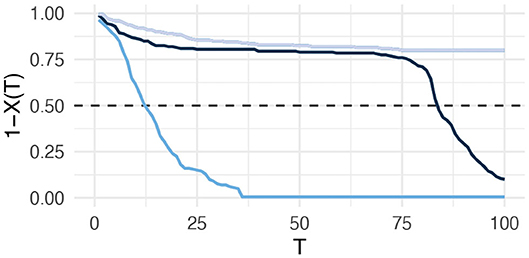
Figure 3. Fraction of firms remaining in the network, 1 − X(T) over time T for different interventions. Driver nodes are chosen from firms with the highest initial knowledge stock (black) or with the highest initial control contribution (gray). Reference case: no node interventions (blue). Parameters: γ = 0.5, b = 0.2, c = 0.06, p = 0.1.
The interactions of firms and the emerging cascades follow a deterministic dynamics. But there are random influences in the way the initial network is generated. For a network of size N, firms randomly connect to N − 1 other firms with a certain probability q. The topology obtained this way also impacts the cascade dynamics. In order to account for this, we have run 100 simulations to find out, when the majority of firms have left, i.e., from each run we determine from the condition and then average over .
Our results show that, without any intervention, the average value is , but the median is = 17. That means in half of all cases was smaller or equal to only 17, which points to a rather left skew distribution and a fast breakdown.
With our interventions, we are able to considerably mitigate this dynamics. Using control contribution as the best ranking scheme, consistently, the average value increases by compared to the case of no interventions, i.e., it doubles. More interesting, the median strongly increases, and in more than half of the runs the maximum time horizon is reached. We used a one-sided Wilcoxon rank sum test with continuity correction for 100 observations, to show that this improvement is statistically significant (p-value ≈ 5.6e − 15).
Using knowledge stock as the ranking scheme for driver nodes also delays large cascades significantly compared to the case without interventions (p-value ≈ 1.86e − 12). But both the average and the median values are slightly smaller than with control contribution as ranking scheme. At the same time, we note that the differences between the two ranking schemes is not really significant (p-value = 0.092). Taking into account the considerable effort in computing the initial control contribution for all firms, we could argue that this effort does not pay off, at least not for the given set of parameters.
Thus, the main difference in mitigating cascades is between no intervention and intervention. For both ranking schemes, the total size of the cascades becomes significantly smaller, i.e., more firms remain in the network, and the occurrence of cascades is also delayed. That means, while we cannot completely prevent cascades of firms leaving, given our set of parameters, we can still reach the aim of our interventions, namely to reduce and to delay them.
4. A Heuristic Approach to Interventions
4.1. Combining Node Level and Network Level Interventions
While the formal approach to node interventions was quite successful, as illustrated above, it also has a number of drawbacks. Cascades were only reduced and delayed, therefore the number of firms in the network necessarily decayed over time. Further, the intervention had to target a larger number of firms. This implies a considerable effort because interventions are costly. First of all, in a real economic network we need to get access to the firms we want to use as driver nodes, and secondly, the control signal itself is also costly. We remind that u is used to lower the costs of those firms that act as driver nodes.
Thus, we would like to have an intervention scenario that uses only a small number of drivers, ideally only one firm, and that compensates for the loss of firms from cascades that could not be prevented. Such a scenario is laid out in the following, and it combines interventions both on the node and on the network level. We call this intervention heuristic because it is not derived in a formal manner but based on intuition and experience. As we will show, it works surprisingly well.
We start by describing the intervention on the network level, or systemic level, which shall be used to compensate for the loss of firms. Here, we consider an instant replacement of firms leaving, such that the total number of firms, N, is kept constant. The new firms create links to randomly chosen partners with a small probability q, hence the expected number of new links is roughly N(T)q, where N(T) = N − Nex(T) is the number of firms in the network after Nex(T) firms left at time T. The random choice of partners is justified by the fact that newcomers do not have complete knowledge about all established firms and their connections.
With this entry-exit dynamics the network topology continuously changes at time scale T. We recall that it has changed already in the first intervention scenario because of firms leaving the network. This has lead to a decreasing number of nodes and links. Now, instead, we have approximately a constant number of nodes and links, but a more pronounced rewiring of the topology resulting from the combined entry and exit of firms.
Interestingly, the fact that a loss of firms is always compensated does not imply that large cascades of firms leaving are prevented. A random addition of new firms does not guarantee that these firms are also well-integrated in the network, therefore they may leave rather soon. So, what is the advantage of this network intervention? It boosts the dynamics of the whole network and occasionally leads to improvements. In fact, firms leaving may open up chances for new firms connecting to the network, and this way generating a better knowledge transfer. Therefore, we keep the random replacement of firms leaving as one element of our intervention scenario, and call it the network intervention. Further, to ensure a continuous network dynamics, we will replace the firm with the lowest even in the rare case that no firm has decided to leave.
We emphasize that the network intervention does not imply any targeted control of firms. Instead, it ensures that the network can constantly evolve on a time scale T. We will later test its impact by comparing our combination of network intervention and node intervention with the previous scenario, the targeted intervention of many firms without network intervention.
4.2. Targeting One Firm
According to the network intervention, firms that leave the network at time step T are replaced by new firms that randomly link to existing firms with a small probability q. This scenario ensures a continuing development both of the network and the knowledge stock of firms. But occasionally it can happen that no firm would decide to leave the network, given the conditions (A) and (B). Then, according to the network intervention, we would replace the firm with the lowest knowledge stock by a new firm that randomly connects to the network, to keep the system dynamics going.
We now propose our node intervention: instead of forcing the firm with the lowest knowledge stock to leave the network, we force a specific firm which we call firm 1, to leave the network, with probability p = 1. We choose as firm 1 a firm that initially belongs to the core of the network. This firm is then replaced by a new firm 1. In case the new firm 1 may no longer be part of the core, we will not apply our node intervention to firm 1 unless it becomes part of the core of the network, again.
This intervention approach sounds very odd, as our aim is to prevent cascades. Firms located at the core of the network have a higher knowledge stock and are often involved in cycles. Therefore their impact on the cascade dynamics is expected to be even larger. This raises two questions. Are we able to “sacrifice” a core firm without enforcing a large cascade? The answer is yes, and it will be illustrated in the small example below. The second and most obvious question is whether such an intervention approach is indeed able to prevent large cascades of firms leaving. The answer is yes, again, although it is quite counter-intuitive. But it is known already from the forest fire model that small forest fires have the ability to prevent large forest fires [37]. Therefore, it makes sense, from time to time, to remove a specific firm from the network in an ordered and controlled procedure, to avoid situations in which large cascades can happen.
To let firm 1 leave the network implies an intervention that brings the knowledge stock of firm 1 below the threshold. We achieve our goal by simply increasing the cost c of only this firm, i.e., c ≡ c + u1δ1,i. The Kronecker delta is δ1, i = 1 only if i = 1 and 0 otherwise. The critical level of u1 is defined by the condition , i.e., u1 depends on the current network, but only needs to be chosen sufficiently large.
4.2.1. An Example
The complexity of our model results from the fact that the network of firms changes on a time scale T, which impacts the possible outcome of the stationary knowledge stocks of all firms. Therefore, we have to resort to numerical investigations. However, for the simple case of only two firms, we are able to provide analytical insights which shall demonstrate that this intervention is indeed able to drive the network dynamics to different states.
Let us assume two firms 1 and 2, where firm 1 is subject of the targeted intervention, as assumed above. Each firm has only one directed link toward the other firm, and the dynamics of their knowledge stocks follows from Equation (1):
If u1 = 0, the stationary knowledge stock of both firms is given as
If u1 ≠ 0, then instead we find for the stationary values
where is a quite involved function of the parameters b, c, u1, and γ, which we print in Appendix A.1. From Equation (4) we find that (i) the values of both and depend on the intervention u1 and (ii) that these values are decreasing functions of u1. That means, for both firms:
The first inequality is understandable since a negative value of u1 would decrease the cost of firm 1, and hence increase its stationary knowledge stock. Because the influence of the intervention u1 propagates from firm 1 to firm 2, we also find an increased stationary knowledge stock for firm 2. Still, the influence of u1 on firm 1 is always stronger:
From Equation (6), we see that for a given threshold xthr > 0, there exist a critical level ũ1 > 0 such that
This is proven in a Theorem presented in the Appendix. That means we can always find a critical level ũ1 for the intervention such that firm 1 would leave the network, but firm 2 would stay in the network, even though it is impacted by the intervention applied to firm 1.
We illustrate the impact of the intervention on firm 1 in Figure 4. It shows the dynamics of the knowledge stock of the two firms with and without intervention by means of two trajectories in a so-called phase plot, (x, y) ≡ (x1, x2). Both firms initially have a knowledge stock above the threshold given by xthr = 1.6. The initial condition is marked by the black dot. Without any intervention, the knowledge stock of both firms would evolve along the dashed red line to the stationary solution marked by the blue cross. The vector field shown indicates this dynamics. However, with an intervention of firm 1, i.e., u1 = 0.2, we are able to drive the dynamics such that it follows the black line and ends up in a stationary solution where , while , indicated by the blue dot. This demonstrates that our intervention to “sacrifice” firm 1, i.e., to force it to leave, indeed works because it will not, at the same time, causes the other firm to leave. Because there is no simple induction from the case of two firms to the case of N firms, we will have to show the efficiency of the heuristic approach by means of computer simulations, presented in the following.
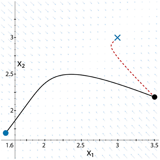
Figure 4. Phase plot illustrating the dynamics of the knowledge stocks x1(t), x2(t) of two firms Equation (2), (red dashed line) u1 ≡ 0, (black solid line) u1 = 0.2.
4.3. Results of Computer Simulations
To illustrate our heuristic approach of combining network interventions and node interventions we choose a rather small network with N = 20. Its evolution is studied over very long time , to check the robustness of the system state achieved by our sinterventions.
Figure 5 shows the network from one run of our simulations, at three consecutive time steps. For the decision of firms to leave we apply condition (A) and a leaving probability p = 1. The color code indicates the stationary knowledge stock of each firm. Light blue means that firms have a value lower than the threshold xthr and thus will leave the network immediately. According to the network intervention, they are replaced by new firms that randomly connect to the network. This part of our intervention scenario is applied at every time step T.
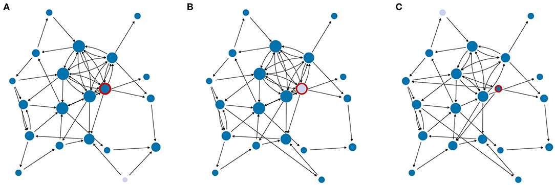
Figure 5. Network evolution with a targeted intervention of firm 1 (always circled in red). Firms with (condition A) (marked in light blue) will leave the network. (A) T = 250, (B) T = 250, and (C) T = 252.
Until T = 250, there were always one or more firms with a low knowledge stock that decided to leave. At T = 251, Firm 1, which was already initially identified as a node from the core of the network, is targeted with an intervention for the first time. The intervals at which such a node intervention becomes necessary fluctuate considerably. Averaging over a long time and many simulations, we find that this intervention happened about every 11 time steps, i.e., in about 11% of network interventions. The control signal forces firm 1 to leave the network, and a new firm 1 enters and randomly links itself to the existing firms. This changes the adjacency matrix and results in new stationary knowledge stocks for all firms. The subsequent snapshot at the next time step is shown in Figure 5C. We note that “sacrificing” firm 1 has resulted in a network with an increased periphery.
What have we gained from this node intervention? First of all, we have ensured that the network dynamics continues, which always has the potential to also reach states of better knowledge exchange between firms. Secondly, we have generated a small cascade of firms leaving. While this seems to be unnecessary at the current point, it may become important at a later time because it may prevent a larger cascade in the future.
To demonstrate this effect, we have plotted, from a single run, the fraction of firms remaining in the network, 1 − X(T), over time T for the cases of (a) only network intervention and (b) combined network and node intervention. The results are shown in Figures 6A,B. We recall that without the network intervention, we would observe a cascade of firms leaving such that the system dynamics ends rather soon (see also Figure 2). With only the network intervention, we can prolong the existence of the network considerably as Figure 6A shows. There are always cascades of firms leaving with varying size. But it takes a considerable long time before the network breaks down completely. Hence, we can conclude that the network intervention alone already allows to delay the breakdown for a time .
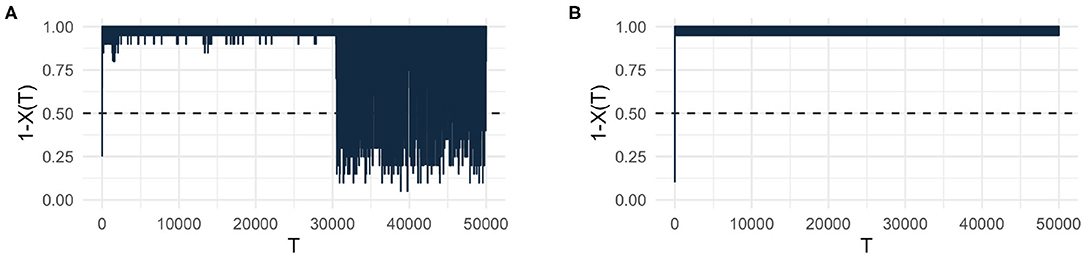
Figure 6. Fraction of firms remaining in the network, 1 − X(T), over time T for different interventions: (A) network intervention only, (B) network interventions and node interventions combined.
This finding can be contrasted with Figure 6B, which shows that a combination of network and node interventions is in fact able to prevent the breakdown of the network, completely. Even for a very long time horizon , we do not notice larger cascades. We remind that cascades always happen at every time step T, but their size is small in case of combined interventions.
Again, to account for random effects in generating the networks we have run 100 simulations to obtain values for , which is the time where the cascade has caused more than 50% of the firms leaving. For the scenario with combined interventions, we always find that , i.e., there is no breakdown observed. But it is still interesting to note the impact of network interventions only. There we find an average value for of about 13,000 time steps, but a median of about 1,300 time steps only. So, again we have a left skew distribution. While there is an improvement of delaying cascades in comparison to the case of no intervention, we can argue that because of the rather small median, this improvement is not large, in particular not if we compare it to the improvement from the combined interventions.
To check the robustness of our results, we have also carried out simulations with N = 250 nodes, a time horizon time steps, and 50 runs. They confirm the findings discussed above. For the combined interventions, we do not observe a breakdown for the given time horizon. Considering network interventions only, we find that both the average and the median are about the same, so instead of a left skew distribution we have a more symmetric one. With 7,100, their value is close to the chosen time horizon. That means, a significant number of runs does not show large cascades during this period. This suggests that network interventions alone become quite efficient for larger networks.
5. Conclusions
Interventions are seen as one important possibility to improve the state of a system. To quantify what kind of interventions would lead to an “improvement” requires an understanding of both the structure and the dynamics of the target system. In this paper, we focus on a collaboration network of firms which exchange knowledge to increase their knowledge stock. Such R&D networks play a vital role in innovation economics and are therefore already studied empirically and theoretically [19, 20, 29, 31]. Hence, our investigations can build on established models for the dynamics of knowledge stock and knowledge exchange. Less studied, so far, are possible intervention scenarios to improve knowledge exchange.
In our paper, we have addressed one particular challenge for the R&D network, namely the fact that firms terminate their collaborations and leave the R&D network if their expectations about knowledge exchange are not met. This is a rational behavior because collaborations are costly, thus the knowledge gain has to overcome some critical threshold. If firms decide to leave the network, this negatively impacts their collaborators and may lead to cascades of firms leaving. With our different intervention scenarios, we want to mitigate this situation. Specifically, to model the decision to leave we have extended previous works by considering not only the firm's knowledge stock, but also their knowledge growth, i.e., their expectations about the development.
Our intervention scenarios follow a bottom-up approach. That means, instead of improving the situation of all firms equally by changing some global conditions, we try to identify a smaller set of firms that should be incentivized. Such firms are called driver nodes in network controllability. Formal approaches to identify minimal sets of driver nodes exist [23, 25, 34–36]. We apply them here for the case of a non-linear dynamics of knowledge growth.
Further, we compare two different ranking schemes for driver nodes. In one case, we choose the 20% of firms with the highest knowledge stock, which are mostly high-degree nodes, in the other case we choose instead the 20% of firms with the highest control contribution, which are often low-degree nodes. Control contribution is a novel node level measure [34] that considers the probability of a node to become a driver node and the size of the subnetwork that is controlled by this node.
If a cascade of firms leaving is about to start, i.e., if 5% of firms already left, driver nodes are incentivized to stay in the network, by lowering their costs by 10%. We emphasize that this is a comparably small intervention, applied to only a small subset of 20% of all firms and only at critical times. But this intervention is sufficient to considerably delay the emergence of a cascade of firms leaving, as the results in Figure 3 demonstrates. We also find that driver nodes chosen for their high control contribution are more effective in preventing cascades of firms leaving.
Our second intervention scenario uses a different approach, by combining interventions on the node and the network level. Network interventions are not targeted at specific firms. Instead, replacing firms that left by new ones that randomly connect to the remaining firms allows a continuous dynamics of the network. This takes into account that random changes can also lead to an improvement. In situations where not much is to lose because cascades already happen, it is certainly worth to be considered.
This intervention alone, however, is not able to prevent cascades of firms leaving, it can only considerably delay them. The reason comes from the fact that new firms are usually not well integrated in the network. Therefore, to improve the situation, we also use a node intervention, but only targeted at one driver node and only at about 10% of all time steps. This firm is forced to leave the network, i.e., instead of reducing the costs, we increase them, for only this firm, such that it is no longer attractive for the firm to stay.
While this intervention seems to be counter-intuitive, it indeed stabilizes the network such that large cascades are prevented, as Figure 6 illustrates. That means, the controlled removal of one firm, chosen the right way at the right time, sustains the network of knowledge transfer if it is combined with the network intervention. The logic of this combined intervention is somewhat similar to the mentioned wildfire prevention [37]. Allowing small wildfires from time to time reduces the risk of a large wildfire considerably. Here, we demonstrate that this logic can be successfully transferred also to an economic context.
Comparing the two different intervention scenarios discussed in this paper, we point to a number of commonalities and differences. First of all, both scenarios are successful, if we consider our minimal aim to prevent large cascades for a certain time horizon . That means, we could buy considerable time to further improve the situation by, e.g., management or policy decisions. The maximal aim, namely to prevent large cascades completely, can be also achieved in the second scenario. But from an economic viewpoint, this might not even be desirable. We remind on Schumpeter's idea of “creative destruction” as an important ingredient of innovation dynamics and economic progress [38]. From this perspective, cascades of firms leaving the collaboration network continuously test the stability, or the viability, of the knowledge transfer system. Preventing the breakdown of an inefficient economic system might have advantages on very short time scales, but definitely hamper its long-term evolution.
A major difference of both intervention scenarios is related to costs. In the first scenario, there is the cost of identifying and accessing the driver nodes, which is not included in our model. But it is obvious that firms with a high knowledge stock, which are mostly nodes with a high degree, are likely more difficult to access and to influence. Then, there is the cost of incentivizing the driver nodes, by lowering their costs, which has to be multiplied by the number of driver nodes. Even if the incentives are small, they can sum up to a considerable amount.
In the second scenario, on the other hand, the intervention is not to reduce the costs of the target firm, but to increase it. Additionally, only one firm needs to be controlled. The network intervention, which is an important part of the second scenario, is not associated with costs for incentives. Instead, the costs involved for the new firms to establish links to the network are covered by these firms.
Eventually, the main reason why the different intervention scenarios have any impact on the knowledge transfer between firms results from the interaction dynamics. Both the positive (reducing the costs) or the negative (increasing the costs) interventions not only impact the knowledge stock of the targeted firms. Because of the network effects underlying the knowledge production, these interventions propagate to other firms and steer the evolution of the whole system toward a desired system state. This state is an emerging property of the system, characterized by a larger robustness against cascades of firms leaving the network.
Data Availability Statement
The original contributions presented in the study are included in the article/supplementary material, further inquiries can be directed to the corresponding author/s.
Author Contributions
FS, YZ, and GC designed the research, wrote the paper, and discussed the results. YZ and GC performed the computer simulations. All authors contributed to the article and approved the submitted version.
Conflict of Interest
The authors declare that the research was conducted in the absence of any commercial or financial relationships that could be construed as a potential conflict of interest.
References
1. Schweitzer F. The bigger picture: complexity meets systems design. In: Folkers G, Schmid M, editors. Design Tales of Science and Innovation. Zurich: Chronos Verlag (2019). p. 77–86.
2. Roberts NC. Tracking and disrupting dark networks: challenges of data collection and analysis. Inform Syst Front. (2011) 13:5–19. doi: 10.1007/s10796-010-9271-z
3. Borgatti SP. Identifying sets of key players in a social network. Comput Math Organ Theory. (2006) 12:21–34. doi: 10.1007/s10588-006-7084-x
4. Heckathorn DD. Respondent-driven sampling: a new approach to the study of hidden populations. Soc Probl. (1997) 44:174–99. doi: 10.1525/sp.1997.44.2.03x0221m
6. Leone Sciabolazza V, Vacca R, McCarty C. Connecting the dots: implementing and evaluating a network intervention to foster scientific collaboration and productivity. Soc Netw. (2020) 61:181–95. doi: 10.1016/j.socnet.2019.11.003
7. Whetsell TA, Siciliano MD, Witkowski KGK, Leiblein MJ. Government as network catalyst: accelerating self-organization in a strategic industry. J Publ Administr Res Theory. (2020) 30:448–64 doi: 10.1093/jopart/muaa006
8. Garcia D, Mavrodiev P, Schweitzer F. Social resilience in online communities: the autopsy of friendster. In: COSN '13: Proceedings of the First ACM Conference on Online Social Networks. Boston: ACM (2013). p. 39–50.
9. Baxter GJ, Dorogovtsev SN, Goltsev AV, Mendes JFF. k-core organization in complex networks. In: Thai MT, Pardalos PM, editors. Handbook of Optimization in Complex Networks. Boston, MA: Springer (2012). p. 229–52.
10. Garas A, Schweitzer F, Havlin S. A k-shell decomposition method for weighted networks. New J Phys. (2012) 14:083030. doi: 10.1088/1367-2630/14/8/083030
11. Hackett A, Melnik S, Gleeson JP. Cascades on a class of clustered random networks. Phys Rev E. (2011) 83:056107. doi: 10.1103/PhysRevE.83.056107
12. Watts DJ. A simple model of global cascades on random networks. Proc Natl Acad Sci USA. (2002) 99:5766–71. doi: 10.1073/pnas.082090499
13. Yu Y, Xiao G, Zhou J, Wang Y, Wang Z, Kurths J, et al. System crash as dynamics of complex networks. Proc Natl Acad Sci USA. (2016) 113:11726–31. doi: 10.1073/pnas.1612094113
14. Lorenz J, Battiston S, Schweitzer F. Systemic risk in a unifying framework for cascading processes on networks. Eur Phys J B. (2009) 71:441–60. doi: 10.1140/epjb/e2009-00347-4
15. Burkholz R, Herrmann HJ, Schweitzer F. Explicit size distributions of failure cascades redefine systemic risk on finite networks. Sci Rep. (2018) 8:6878. doi: 10.1038/s41598-018-25211-3
16. Burkholz R, Leduc MV, Garas A, Schweitzer F. Systemic risk in multiplex networks with asymmetric coupling and threshold feedback. Phys D. (2016) 323–4:64–72. doi: 10.1016/j.physd.2015.10.004
17. Schweitzer F, Fagiolo G, Sornette D, Vega-Redondo F, White DR. Economic networks: what do we know and What do we need to know? Adv Compl Syst. (2009) 12:407–22. doi: 10.1142/S0219525909002337
18. Saavedra S, Reed-Tsochas F, Uzzi B. Asymmetric disassembly and robustness in declining networks. Proc Natl Acad Sci USA. (2008) 105:16466–71. doi: 10.1073/pnas.0804740105
19. Tomasello MV, Napoletano M, Garas A, Schweitzer F. The rise and fall of R&D networks. Indus Corpor Change. (2016) 26:617–46. doi: 10.2139/ssrn.2749230
20. Powell WW, White DR, Koput KW, Owen-Smith J. Network dynamics and field evolution: the growth of interorganizational collaboration in the life sciences. Am J Sociol. (2005) 110:1132–205. doi: 10.1086/421508
21. Haynes GWG, Hermes H. Nonlinear controllability via lie theory. SIAM J Control. (1970) 8:450–60. doi: 10.1137/0308033
22. Sussmann HJ, Jurdjevic V. Controllability of nonlinear systems. J Differ Equat. (1972) 12:95–116. doi: 10.1016/0022-0396(72)90007-1
23. Liu YY, Slotine JJ, Barabasi AL. Controllability of complex networks. Nature. (2011) 473:167–73. doi: 10.1038/nature10011
24. Whalen AJ, Brennan SN, Sauer TD, Schiff SJ. Observability and controllability of nonlinear networks : the role of symmetry. Phys Rev X. (2015) 5:011005. doi: 10.1103/PhysRevX.5.011005
25. Cornelius SP, Kath WL, Motter AE. Realistic control of network dynamics. Nat Commun. (2013) 4:1942. doi: 10.1038/ncomms2939
26. Casiraghi G, Schweitzer F. Improving the robustness of online social networks: a simulation approach of network interventions. Front Robot AI. (2020) 7:57. doi: 10.3389/frobt.2020.00057
27. Gassmann O, von Zedtwitz M. New concepts and trends in international R&D organization. Res Policy. (1999) 28:231–50. doi: 10.1016/S0048-7333(98)00114-0
28. Schweitzer F. The law of proportionate growth and its siblings: applications in agent-based modeling of socio-economic systems. In: Aoyama H, Aruka Y, Yoshikawa H, editors. Complexity, Heterogeneity, and the Methods of Statistical Physics in Economics. Tokyo: Springer (2020). Available online at: https://arxiv.org/abs/1909.00653
29. Koenig MD, Battiston S, Schweitzer F. Modeling evolving innovation networks. In: Pyka A, Scharnhorst A, editors. Innovation Networks. New Approaches in Modelling and Analyzing. Berlin: Springer (2009). p. 187–267. Available online at: http://link.springer.com/10.1007/978-3-540-92267-4_8 http://www.springerlink.com/index/10.1007/978-3-540-92267-4 http://arxiv.org/abs/0712.2779
30. Nowak MA, Sigmund K. The dynamics of indirect reciprocity. J Theor Biol. (1998) 194:561–74. doi: 10.1006/jtbi.1998.0775
31. Abrahamson E, Rosenkopf L. Social network effects on the extent of innovation diffusion: a computer simulation. Organ Sci. (1997) 8:289–309. doi: 10.1287/orsc.8.3.289
32. Jain S, Krishna S. Autocatalytic sets and the growth of complexity in an evolutionary model. Phys Rev Lett. (1998) 81:5684. doi: 10.1103/PhysRevLett.81.5684
33. Zhang Y, Garas A, Schweitzer F. Value of peripheral nodes in controlling multilayer scale-free networks. Phys Rev E. (2016) 93:012309. doi: 10.1103/PhysRevE.93.012309
34. Zhang Y, Garas A, Schweitzer F. Control contribution identifies top driver nodes in complex networks. Adv Complex Syst. (2019) 22:1950014. doi: 10.1142/S0219525919500140
35. Jia T, Barabási AL. Control capacity and a random sampling method in exploring controllability of complex networks. Sci Rep. (2013) 3:2354. doi: 10.1038/srep02354
36. Wang B, Gao L, Gao Y. Control range: a controllability-based index for node significance in directed networks. J Stat Mech. (2012) 4:P04011. doi: 10.1088/1742-5468/2012/04/P04011
37. Zinck RD, Grimm V. Unifying wildfire models from ecology and statistical physics. Am Nat. (2009) 174:E170–85. doi: 10.1086/605959
A. Appendix
A.1. Explicit Stationary Solutions
Here we provide the detailed expressions for the stationary knowledge stocks of a network with only two firms 1,2. Their dynamics was given in Equation (2) and their stationary solutions in Equation (4), which we repeat here:
The function reads explicitely:
with k given by:
and m given by:
A.2. Theorem for Controlling Two Firms
Equation (6) states that, given a threshold xthr > 0, we can always find a critical value of the intervention ũ1 such that the stationary knowledge stock of firm 2 (without intervention) is above the threshold, while the knowledge stock of firm 1 (targeted by the intervention) is below the threshold. We can formalize this statement in a simple theorem.
Theorem 1. Let xthr > 0 be a threshold and be the stationary knowledge stocks of firms i ∈ {1, 2,} with a control signal u ∈ ℝ applied to firm 1. Then, as long as , there is a value ũ∈ℝ such that:
In the following, we provide a sketch of its proof. There are two possible cases:
The first case is trivial. Choosing ũ = 0 is the solution. For the other case, we use the expressions given in Equations (4) and (A1). With i ∈ {1, 2}, we can see as monotonously decreasing and continuous functions of u ∈ [0, ∞). Hence, they are also bijective functions within this interval. According to Equation (6), then, there exist a positive ũ such that Equation (A4) is satisfied.
Keywords: network, control, robustness, failure cascade, agent-based model (ABM)
Citation: Schweitzer F, Zhang Y and Casiraghi G (2020) Intervention Scenarios to Enhance Knowledge Transfer in a Network of Firms. Front. Phys. 8:382. doi: 10.3389/fphy.2020.00382
Received: 25 June 2020; Accepted: 07 August 2020;
Published: 18 September 2020.
Edited by:
Andrea Rapisarda, University of Catania, ItalyReviewed by:
Michele Bellingeri, University of Parma, ItalyYuyao Wang, Nanjing University of Science and Technology, China
Copyright © 2020 Schweitzer, Zhang and Casiraghi. This is an open-access article distributed under the terms of the Creative Commons Attribution License (CC BY). The use, distribution or reproduction in other forums is permitted, provided the original author(s) and the copyright owner(s) are credited and that the original publication in this journal is cited, in accordance with accepted academic practice. No use, distribution or reproduction is permitted which does not comply with these terms.
*Correspondence: Frank Schweitzer, fschweitzer@ethz.ch