Delineation of Radar Glacier Zones in the Antarctic Peninsula Using Polarimetric SAR


Key Lab of Digital Earth Science, Aerospace Information Research Institute, Chinese Academy of Sciences, Beijing 100094, China
*
Author to whom correspondence should be addressed.
Water 2020, 12(9), 2620; https://doi.org/10.3390/w12092620
Submission received: 7 August 2020
/
Revised: 31 August 2020
/
Accepted: 12 September 2020
/
Published: 18 September 2020
(This article belongs to the Section Hydrology)
Abstract
:Climate change is a cause of the expansion of snowmelt phenomena in the Antarctic, and shifts in position of wet and dry snow lines have been considered as good indicators of climate changes. The impacts of climate change are observable by the delineation of significant position change of glacier zones. The principal limitation of current glacier zone classification methods by synthetic aperture radar (SAR) image is that it is difficult to discriminate dry-snow and wet-snow zones using only single-polarimetric radar backscattering intensity. This study tried to solve the problem using polarimetric SAR (PolSAR). Analysis indicates that polarimetric decomposition elements could be efficient characteristics to delineate radar glacier zones by recognition of principal backscatter patterns. Further, two radar glacier zone classification processes for polarimetric SAR are proposed: a supervised support vector machine (SVM) classification process and a simple decision-tree classification method. These methods enable reliable delineation of radar glacier zones in the Antarctic Peninsula. Polarimetric SAR, which provides more information about the scattering processes and target structure, proves to be an efficient tool for delineating radar glacier zones and snowmelt detection.
1. Introduction
As concern about global climate change becomes more widespread, Antarctic glaciers, which play a major role in the cryosphere and planetary system, are experiencing an expansion of surface melting [1,2]. Antarctic glacier snowmelt has a drastic influence on the behavior of the ice sheet, influencing the absorption of solar radiation and the thermal exchange between the ground surface and the atmosphere. Antarctic snowmelt is also an indicator of global warming as the snowmelt activity is very sensitive to slight changes in atmospheric temperature [3].
It is difficult to carry out manual surveys in Antarctica. However, along with the rapid development of satellite remote sensing, an enormous amount of effort is going into studying Antarctic snowmelt using remote sensing: this research mainly uses microwave remote sensing, which has a superior ability to monitor glaciers and ice shelves [4,5,6,7,8]. Sophisticated algorithms for detecting and estimating snowmelt using passive microwave sensors have been proposed [9,10], and microwave radiometers, together with microwave scatterometers, are widely used in low-resolution snowmelt observations [3,11,12]. Active microwave remote sensing has been proved to be sensitive for making glacier observations [13,14,15], and, compared with passive microwave remote sensing, synthetic aperture radar (SAR) images display higher spatial resolution, which enables us to achieve fine observations of glacier snowmelt and glacier zones, as has also been demonstrated in recent years [16,17,18,19,20].
Glacier zones are the result of precipitation falling as snow followed by ice formation, snowmelt, and refreezing, and they have proved to be an important indicator of climate change [12,18,21]. In SAR images, backscatter from snow and ice surface depends on snow density, liquid water content, grain size, stratigraphy, and surface roughness [22,23]. Different snow zones on a glacier are identifiable on SAR images [24,25]. Previous simulation research suggested that a frozen percolation radar zone experiencing heavy snowmelt in summer turns bright on SAR images in winter, whereas the dry snow radar zone with high accumulation is dark [26]. These radar glacier zones, including wet snow, frozen percolation, dry snow, superimposed ice, and bare ice radar zone, can be classified by backscattering coefficient and elevations [22]. The wet snow line—the line between the wet snow radar zone (WSRZ) and the frozen percolation radar zone (FPRZ)—is an indicator of the current snowmelt situation caused by rising air temperatures, while the dry snow line—the boundary of the dry snow radar zone (DSRZ)—is an indicator of the extreme climate warming and snowmelt activity that has occurred in recent years [27,28].
Current studies concentrate on glacier zone classification and boundary drawing using only single-polarimetric (single-pol) radar scattering intensity, seldom making use of the analysis of polarimetric SAR (PolSAR), which can provide more abundant information to reflect the different scattering mechanisms [29,30,31]. In existing glacier zone classification methods using single-pol SAR, it is difficult to distinguish dry- and wet-snow zones for their similar backscattering characteristics in only single-pol radar backscattering intensity [1,18,21]. The novelty of this study compared to previous research is that it discriminates DSRZ and WSRZ using full-polarimetric SAR data. We firstly analyze the backscattering characteristics of different glacier zones using satellite SAR, in particular, PolSAR. Then, two classification methods that use polarimetric decomposition were proposed to discriminate dry and wet glacier zones. Finally, an experiment was performed to identify glacier zones using full-polarimetric Radarsat-2 data in the Antarctic Peninsula, where the glacier melt occurs most frequently in the southern summer.
2. Study Area and Datasets
Considering that snowmelt is a regionally variable phenomenon affected primarily by air temperature, the Antarctic Peninsula, with its complex terrain and varied snowmelt conditions, was chosen for this study. The datasets include 17 ENVISAT—ASAR wide-swath images with HH polarization acquired from December 2010 to January 2011 by the European Space Agency (ESA) and two Radarsat-2 WSM (wide ScanSAR mode) dual-polarimetric images (HH/HV and VV/VH) acquired in January 2014, which were used to analyze the backscattering characteristics of glacier zones in different states. The ASAR and Radarsat-2 images were obtained using ScanSAR technology in order to achieve extra-wide-swath coverage with a swath of about 450–500 km. In addition, the digital elevation model (DEM) data from MAMM (Modified Antarctic Mapping Mission), retrieved by ICEsat (Ice, Cloud, and land Elevation Satellite) altimeter and Aster satellite stereo imagery, were also used in this study.
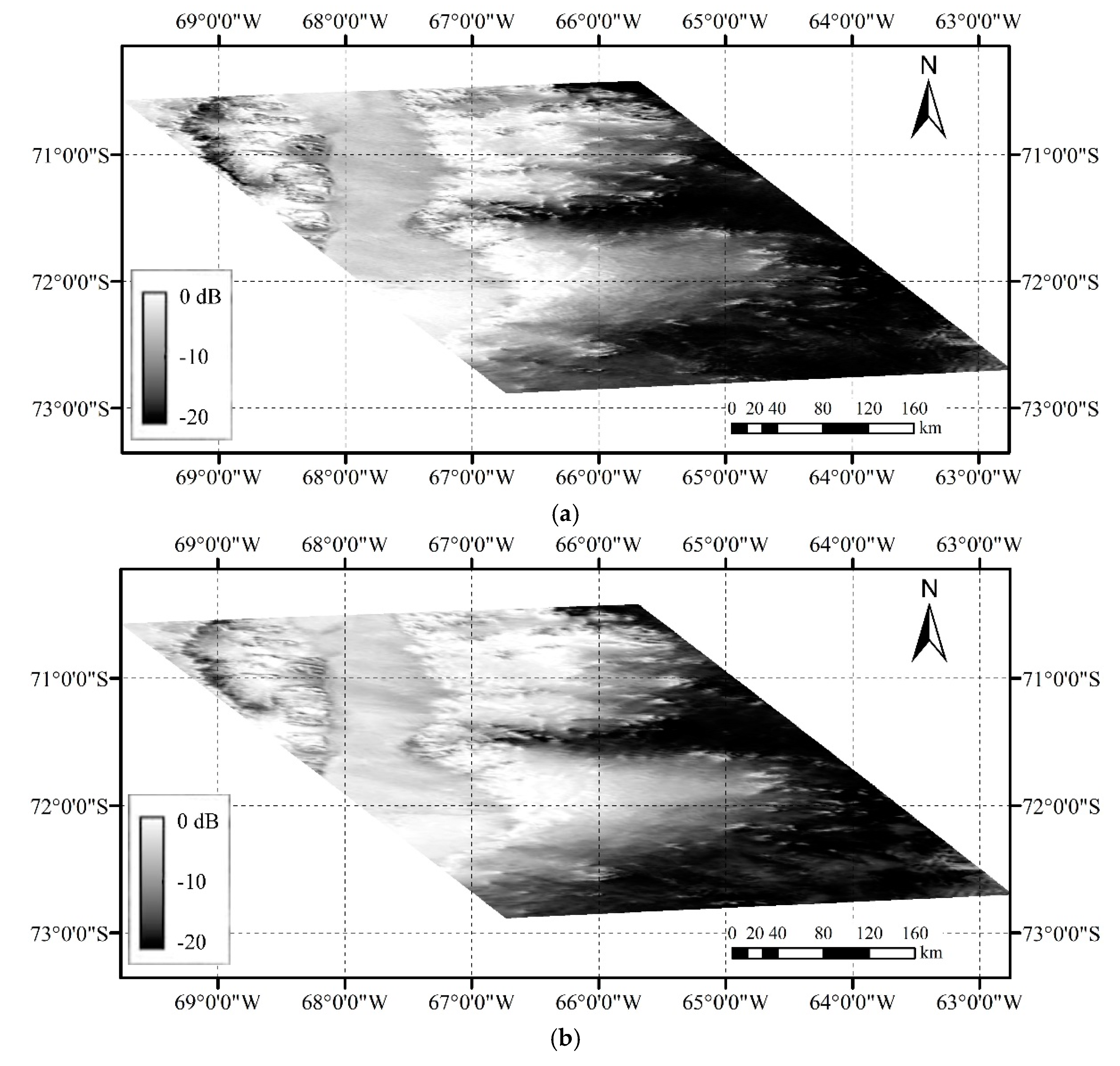
In this study, the Single Look Complex (SLC) images were multi-looking processed (window size 5 × 5) to reduce coherent noise, and then local incidence angle compensation was used to acquire the backscatter coefficient, γ0, corrected for the effects of the beam incidence angle and terrain [32,33]:
where α is the local incidence angle for the pixel used in the terrain correction. The preprocessing was performed using open-source SNAP (The Sentinel Application Platform) toolbox. The ASAR images before and after preprocessing are shown in Figure 1.
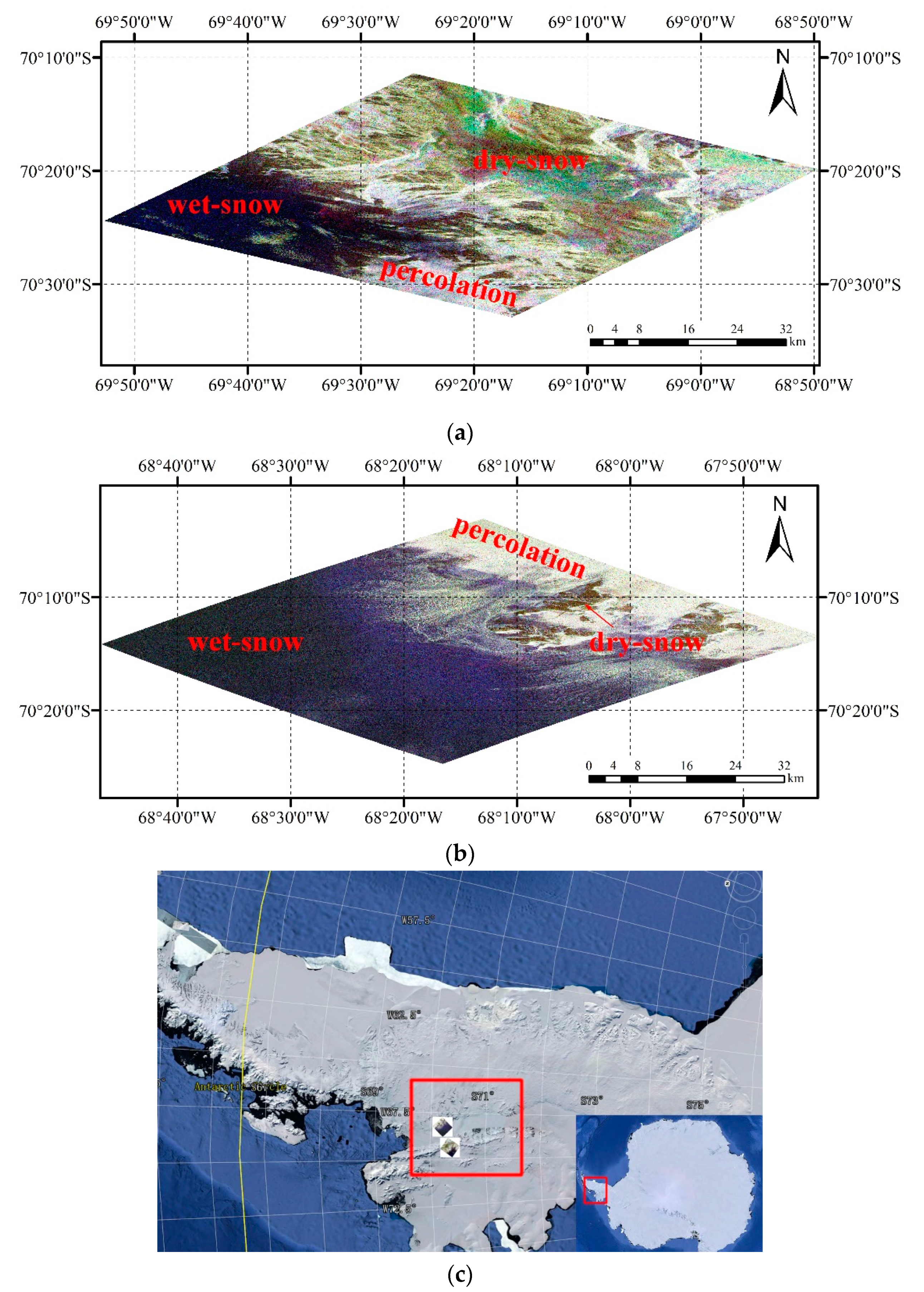
The full-polarimetric imagery used in this study consisted of two Radarsat-2 images used to study the glacier zone classification methods by polarimetric SAR data. They were acquired on 24 January 2014 and 5 January 2015, meaning that both were acquired during the melt period. The Single Look Complex (SLC) imagery was used here for polarimetric decomposition and analysis (Figure 2). In Figure 2, it can be seen that the different snow zones have distinct characteristics in the Pauli images. The parameters of the Radarsat-2 dataset are shown in Table 1.
3. Radar Glacier Zones and the Backscattering Characteristics
3.1. Radar Glacier Zones
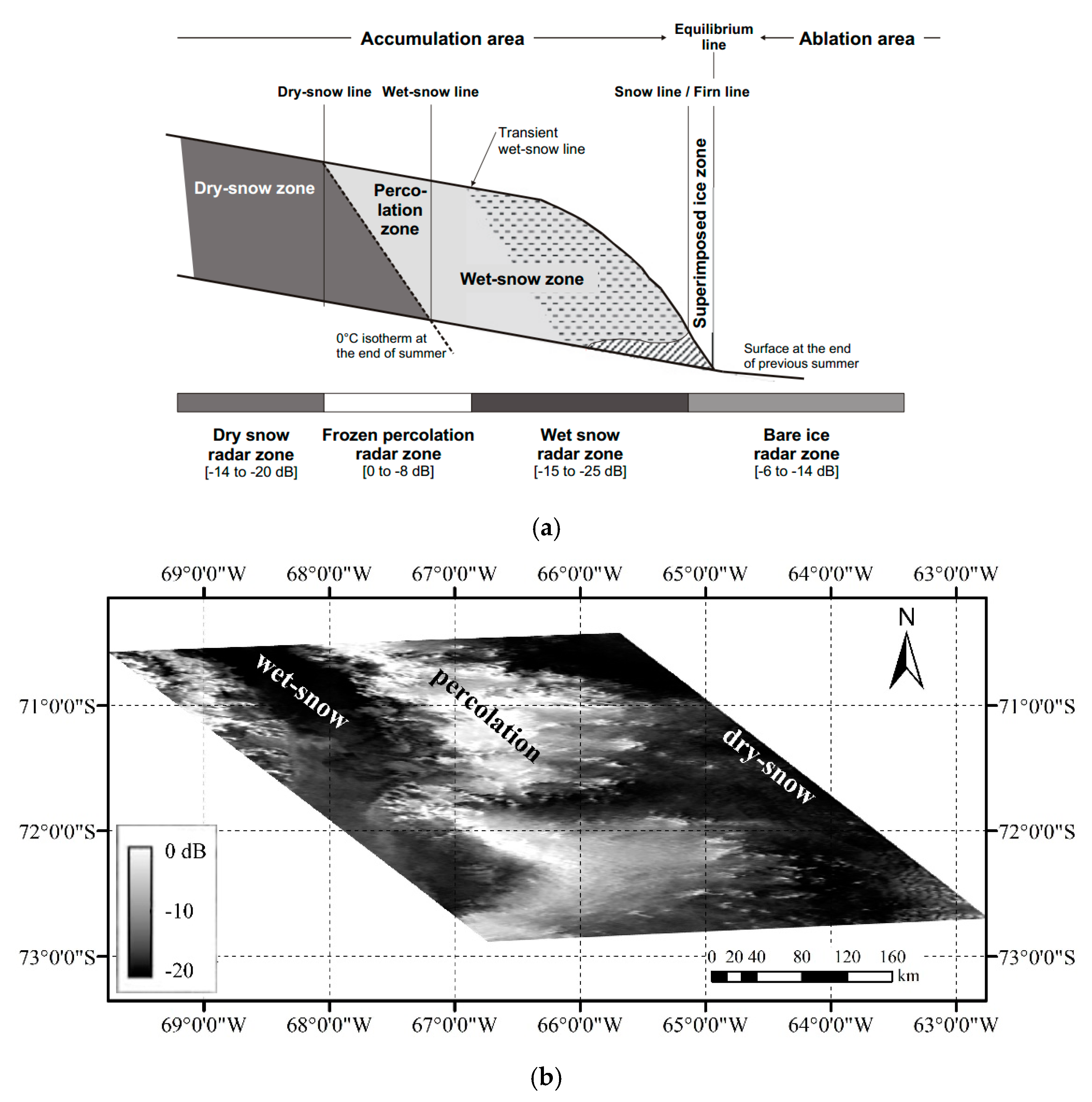
Classical glacier zones, which differ according to snow status and structure, result from variations in precipitation, air temperature, and the freeze–thaw process. Benson’s glacier classification concept is used here without strictly separating glacier zones from glacier facies—although the two concepts are not strictly equivalent in cryology [22]—which is shown in Figure 3a.
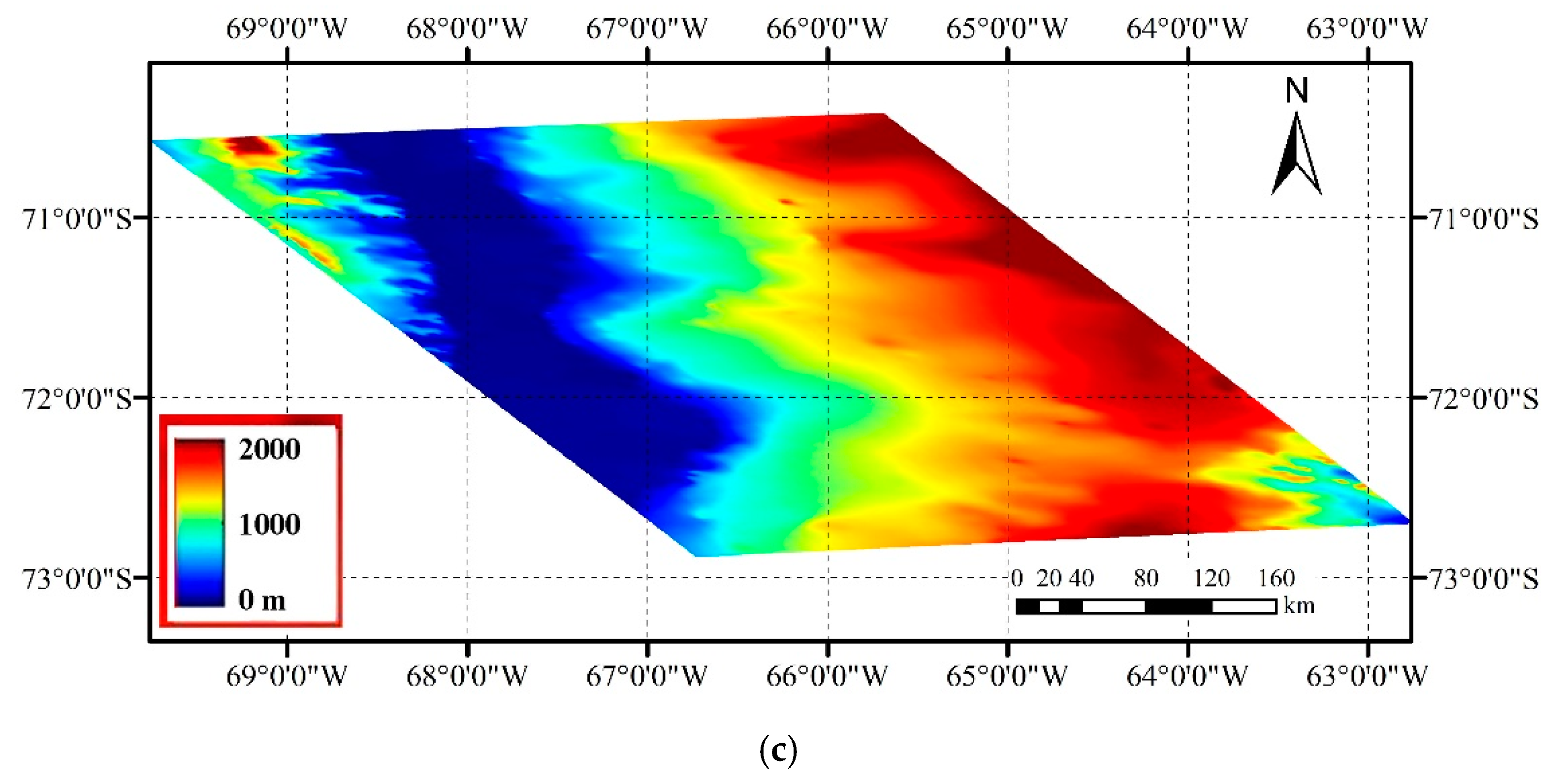
Glacier facies are typically recognized as consisting of four zones [21,22,27]: (1) the dry snow facies (dry snow radar zones) above the dry snow line, where negligible melt occurs in the interior; (2) the percolation facies (frozen percolation radar zone) between the dry snow line and the wet snow line, where meltwater infilters and freezes, forming a reticulation of pipe-like percolation channels, ice glands, lenses, and layers; (3) the soaked snow facies (wet snow radar zone) below the wet snow line, where meltwater soaks the surface and subsurface; and (4) the ablation facies (bare ice radar zone, BIRZ) below the firn line, is usually located at the end of ice sheet connected to sea ice [22], where no snow accumulates above the bare ice. The glacier zones in SAR image are shown in Figure 3b and the corresponding DEM in Figure 3c, and it can be seen that dry-snow and wet-snow zones have similar backscattering intensity. In the Antarctic Peninsula, the BIRZ occurs mainly in low latitude areas during the short melt season and is often difficult to distinguish from the wet-snow zones (in summer) and sea ice. In this study, therefore, the BIRZ was ignored.
The boundaries between the glacier zones provide information on the snowmelt and mass balance. The dry-snow line is often stable over a timescale of years and is an indicator of individual historical extreme melting events [22]. The transient wet snow line, which approximately coincides with the freezing-point isotherm, reflects the current melt extent. The elevations of the dry- and wet-snow lines in Figure 3b are about 1200 and 600 m, respectively. The firn/snow line separating the BIRZ and WSRZ (summer) or FPRZ (winter) often coincides with the equilibrium line—the zero glacier mass-balance line—at the end of the ablation season.
3.2. Backscattering Characteristics
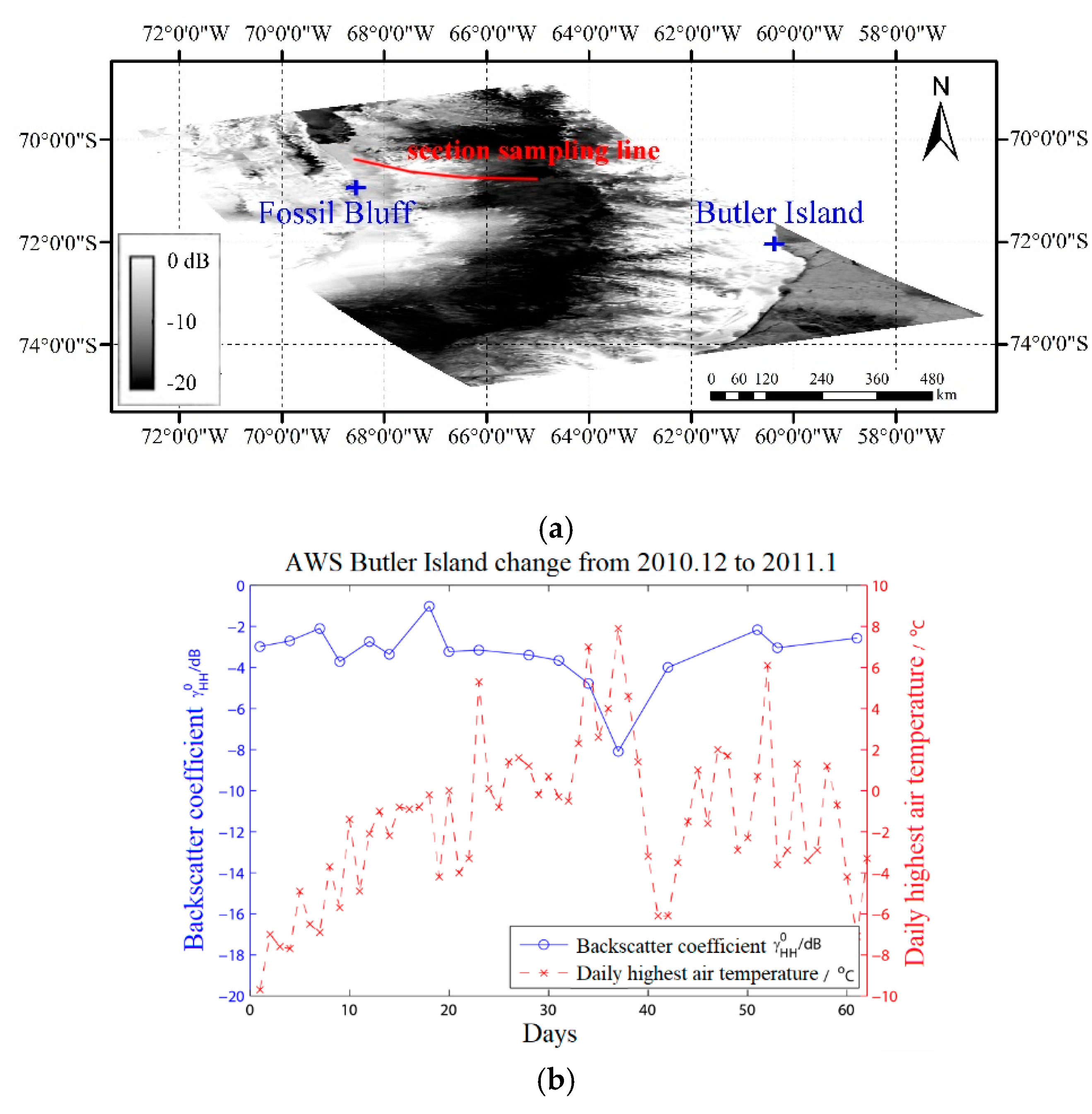
Different precipitation and freeze–thaw processes result in distinct glacier zones, which appear as strips in SAR imagery. The backscattering characteristics of radar glacier zones were sampled and analyzed (Figure 4a) using multi-temporal wide-swath ASAR imagery.
Microwave energy is extenuated by long-distance transmission in thick but puff snow, which leads to weak reflectance power and low backscatter intensity of DSRZ in SAR imagery, typically as permanent firn snow in high-altitude areas. In FPRZ, ice structures, e.g., ice lens and pipes formed by faint surface melting and percolation refreezing inside, cause strong high backscatter coefficient (γ0) or sigma naught (σ0). According to Rau [23], FPRZ σ0 values range between −8 and 0 dB. The WSRZ and DSRZ σ0 values are lower than for the FPRZ, but both have a wide distribution of values, especially for wet snow during the severe ablation season, and so there are no definite values of σ0. Rau gave typical ranges of σ0 for the WSRZ and DSRZ as −15 to −25 dB and −14 to −20 dB, respectively.
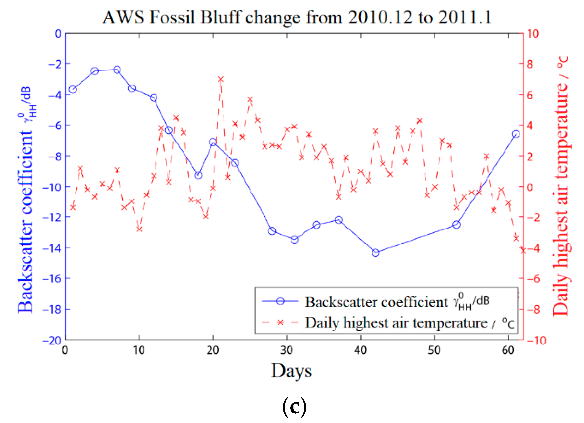
In summer, snowmelt in the FPRZ (in winter) lowers the σ0 by a large amount, which can be seen in the multi-temporal SAR imagery. Figure 4b,c shows the change at the two automatic weather stations shown in Figure 4a. Figure 4c clearly shows an almost complete dry melting–freezing cycle: the change in the radar backscatter lags behind the air temperature slightly.
4. Methodologies
4.1. Identifying Radar Glacier Zones with Polarimetric SAR
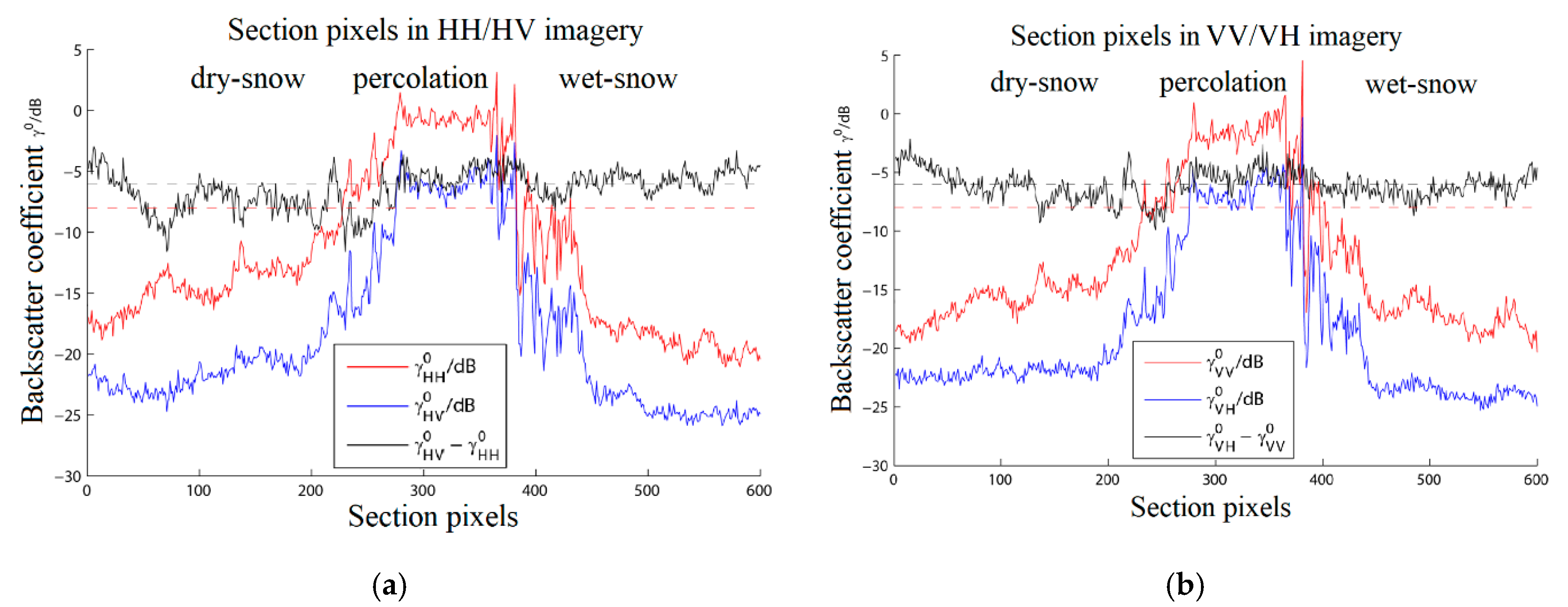
Using two Radarsat-2 wide-swath dual-polarimetric images, the characteristics of the backscatter coefficients of radar glacier zones in different polarimetric channels (HH/HV and VV/VH) were analyzed. Figure 5 shows the transition (the sampling line in Figure 4a) of the radar backscatter coefficient from dry snow to wet snow in four different polarimetric channels. The x-axis is a surface cross-section of steep descending slope with the snowmelt status from dry to intensely melting snow.
Owing to the sensitivity of the snow’s water content and dielectric constant to the microwave scattering process, the decrease in backscatter intensity from dry snow or wet snow to the percolation zone can be easily identified.
Unlike the coherent scattering procedure obviously differing in cross-polarized and co-polarized channels, the value of γ0 for radar glacier zones in cross-polarized imagery is similar to that for co-polarized imagery. In terms of the identification of radar glacier zones, the cross-polarization γ0 is virtually equivalent to the co-polarization γ0 but has an absolute value that is about 6 dB lower.
The DSRZ or WSRZ can easily be discriminated from the FPRZ using backscatter intensity: for several decomposition types (such as Yamaguchi and Freeman–Durden decomposition [29]), the difference is more obvious for the enhanced intensity components (such as HH + VV in the Pauli basis) and volume scattering components. The decrease in backscatter intensity from FPRZ to DSRZ or WSRZ results from different microwave scattering processes: the backscattering in the DSRZ is dominated by weak volume scattering, whereas, in the WSRZ, the amount of volume scattering falls sharply and the backscattering is dominated by surface scattering.
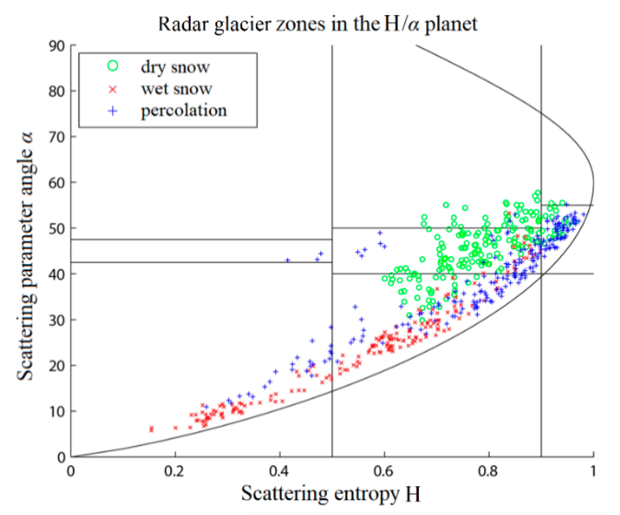
Using Cloude decomposition, the polarimetric entropy and scattering angle can be used to recognize the dominant scattering mechanism and depolarizing property [34,35]. Microwave backscattering anisotropy seems not to be effective in glacier zone recognition due to the dominant distributed volume scattering. As shown in Figure 6, FPRZ sample pixels were located mainly in areas of medium or high entropy, which accounts for the high or medium levels of multiple scattering or volume scattering. The DSRZ is similar to the FPRZ, being dominated by volume scattering from percolation, corresponding to volume or multiple scattering. In the WSRZ, the sampled pixels in the medium entropy areas suggest weakly depolarizing scattering mixed with surface scattering and volume scattering. The scattering process in the lower entropy areas is mainly due to a pure single target, where the point scattering can be considered as the dominant scattering mechanism [29,36].
4.2. Classification Methods
It is easy to recognize the FPRZ from its high backscattering coefficient in SAR imagery. The transition from percolation to wet snow or dry snow can be easily deduced from the decrease in scatter intensity using prior knowledge. However, isolated areas of low backscattering are difficult to recognize as being the DSRZ or WSRZ even using the polarization ratio (the polarization deviation, measured in dB). As the use of texture information from glacier distribution scattering is seldom effective, it is difficult to directly recognize radar glacier zones. Other information, such as the altitude or images, has been used to solve this problem in some studies [21,23]. Several authors have tried different altitude thresholds to divide the map into two areas: a lower-altitude area that includes only percolation and wet snow and a highland area where, due to the low temperature, the snow is probably dry. This simple hypothesis is not appropriate for polar glaciers with rugged topography and complex weather conditions, and the threshold is also not universal for different flat glacier areas. In our previous work, the use of altitude thresholds was attempted in part of the Antarctic Peninsula, and the use of equivalent cross-polarization threshold means for classifying radar glacier zones was proposed. We also proposed another approach using previously acquired winter imagery to extract dry snow areas using a change detection technique [37]. Because of the stability of the DSRZ, this technique was effective over the short period since the winter imagery was acquired.
The distinct backscatter characteristics of glacier zones are similar in co-polarized and cross-polarized imagery, which causes difficulty in the delineation of glacier zones. Complex terrain and weather conditions in polar glaciers cause the distribution of glacier zones to be irregular. The indirect methods described above do not always work, which makes it necessary to delineate glacier zones using SAR image characteristics. Polarimetric SAR target decomposition, which produces more scattering process information, as described above, could be helpful in recognizing glacier zones by analyzing the dominant backscatter mechanism.
The major problem is the similarity between the WSRZ and DSRZ, which makes it difficult to classify radar glacier zones using the backscattering intensity of co-polarized and cross-polarized imagery. However, polarimetric decomposition analysis produces a complete contrast between the WSRZ and DSRZ in terms of the scattering mechanism. Two methods for classifying radar glacier zones using polarimetric SAR decomposition are proposed in this paper: a supervised support vector machine (SVM) classification procedure and a simple decision classification-tree method.
(1) Supervised SVM classification
General polarimetric SAR decompositions can provide many components, which can be useful in glacier zone classification. Following a specific selection procedure, different decomposition components can be used as inputs to a classifier. The procedure for supervised SVM classification described below is also illustrated in Figure 7a, and the software package LIBSVM (https://www.csie.ntu.edu.tw/~cjlin/libsvm/) was used in this method.
1. Statistical information and sampling information for glacier zones were acquired from dozens of decomposition components derived from Pauli decomposition, Cloude–Pottier decomposition, and Touzi decomposition [38]. These decomposition components, which were the candidates for the following classification, were acquired from these general polarimetric decompositions. The components derived from Touzi decomposition and H/A/α decomposition can be found in [34,39], respectively. Pauli decomposition and Cloude decomposition can be expressed as follows [29]:
Pauli decomposition:
Cloude decomposition:
where the coherence matrix T is a 3 × 3 Hermitian matrix. The superscript T denotes the transpose operation, † is the conjugate transpose, and denotes the ensemble average. Λ is a real diagonal matrix and contains the eigenvalues of T, and λ1 > λ2 > λ3. U contains the eigenvectors.
2. Nine hundred sampling points were selected from different decomposition components, according to the above backscattering characteristics of WSRZ and DSRZ, while simultaneously considering the elevation information. Then, the differences d between the mean values of the two classes for each decomposition component were calculated [40]:
where uWSRZ and uDSRZ are the averages of the sample points for class WSRZ and DSRZ, and σWSRZ and σDSRZ are their respective standard deviations.
Here, the parameter d describes the overall degree of separation for each classification parameter. Candidate parameters with d < 0.4 were discarded as being inefficient and interfering factors for the classification (these parameters are not shown in bold in Table 2).
3. The correlation coefficients between pairs of parameters were compared; this reduces the amount of redundant similar information.
Candidate parameters that were too similar (correlation coefficient for the pair greater than 0.8) increased the amount of work for the classifier. In this method, parameters that had a small variance between them were discarded (Table 3).
In Table 3, one candidate is discarded from the pair with the correlation coefficient greater than 0.8. Then, as shown in Table 3, four candidates were selected after the selection Steps 2 and 3, shown in bold in the table. Owing to the scattered distribution of glacier zones, Freeman decomposition produces a large number of invalid pixels, thus this decomposition method was not considered for use in the classification [41,42].
4. The supervised SVM classifier was applied. The selections produced by the above procedure were considered to be efficient parameters for use in glacier zone classification. An SVM classifier, which is widely considered as a robust classifier for general classification where there are few samples available for a non-linear problem [43], was applied here.
In this example, Cloude components λ1, λ2, and λ3, together with the polarimetric scattering angle, α, were considered to be optimal classification candidates and used as inputs to the SVM classifier. The excluding thresholds and final selected candidates are shown for reference only.
(2) Decision classification tree method
As the PFRZ is easily distinguishable in SAR imagery and Cloude decomposition can efficiently recognize the important scattering mechanisms, a simple decision-tree classification procedure that uses an H-α plane (Figure 7b) is proposed.
1. FPRZ extraction using a backscatter intensity threshold. As the strongest volume backscattering originates from crystal structures in the percolation zones, the FPRZ is characterized by the highest backscattering coefficient. According to the results of former studies in glacier zones, −8 dB (equivalent to −14 dB for the cross-polarization channel) is a credible co-polarization channel threshold for extracting the FPRZ. Simply using a threshold of −8 dB for the calibrated HH imagery enables the extraction of the FPRZ to be extended.
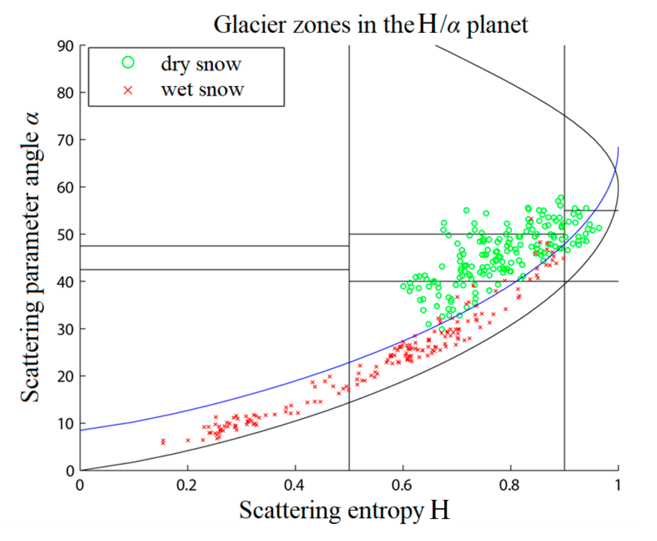
2. WSRZ and DSRZ delineation in the H-α plane. In the H-α plane, the dry-snow zone can be distinguished from the wet-snow zone using the dominant scattering type. The wet-snow zone pixels are located close to the lower boundary of the H-α plane, meaning that a curve parallel to this boundary (which crosses the midpoint of the high-entropy boundary (0.9, 45)) separates the dry-snow and wet-snow zones well [29].
The dividing line in Figure 8 parallel to the lower boundary is a reference curve derived from sample pixels. The intercept of this line is determined by minimizing the product of the misclassification probabilities of the sampling points of dry snow and wet snow.
5. Results and Discussion
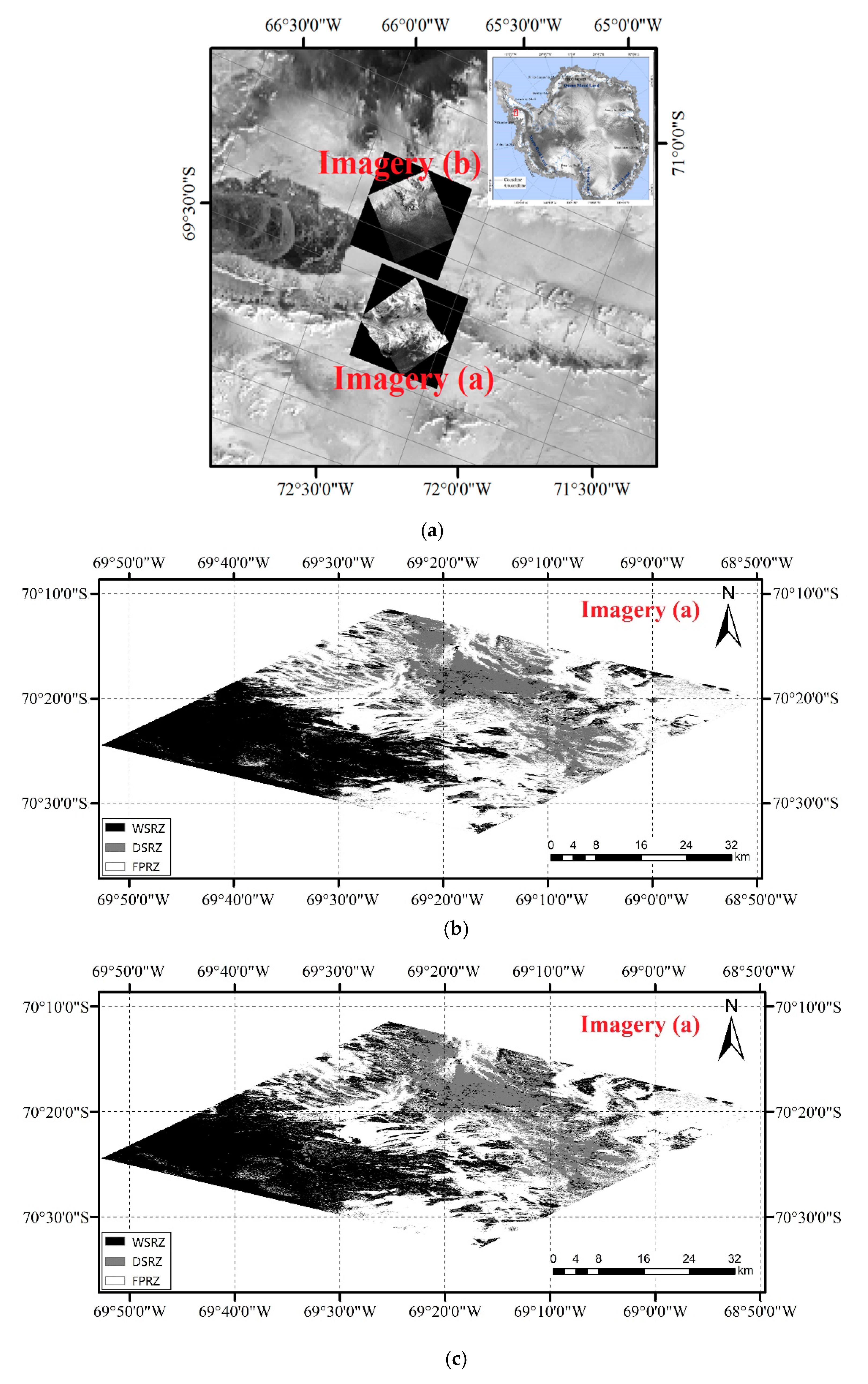
Figure 9 shows the results of glacier zone classification obtained using the two polarimetric SAR classification methods described in this paper. Figure 9a shows the locations of Images (a) and (b). Image (a) is located across a narrow ridge on the Antarctic Peninsula. The upper half is a percolation zone at a high elevation, while the lower half is an area of rapid melting. This is a dry-snow zone in the high mountains (highest elevation above 1500 m), and percolation zones can be seen clearly outlined on both sides. The mean elevation of the transition from the percolation zone to the dry snow zone in this image is about 1200 m. A zone of melting wet snow lies near the glacier edge in the lower-left corner of the image.
In general, a full-polarimetric SAR image covers a much smaller area than a ScanSAR image. It is difficult to get validation points from auto weather station record or passive microwave detection result [4]. As known from former studies, snowmelt status can be presumed approximately from elevation (correlated to air temperature) and backscatter intensity. Thus, the sampling points from current SAR imagery were used in this study for result validation, and classification confusion matrix and kappa coefficient were used here.
Figure 9b shows the result for the supervised SVM classification using Image (a). The supervised classification procedure using polarimetric SAR decomposition produced good glacier zone classification results, with an overall accuracy of 91.8% and kappa coefficient of 0.876 for these sample areas (Table 4). Supervised classification thus proved to be a reliable method for the delineation of glacier zones.
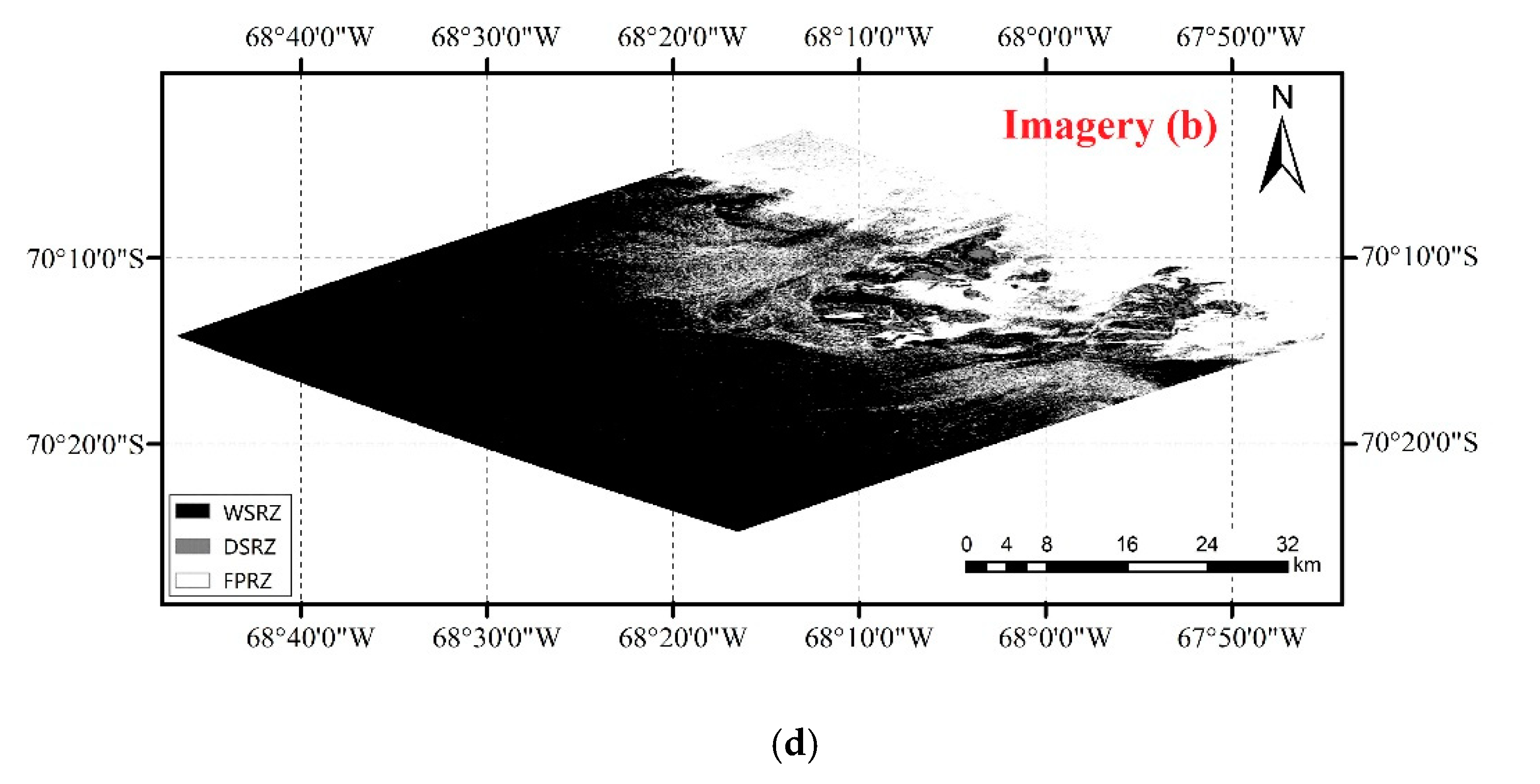
The decision classification tree method is a simple unsupervised classification method, which requires little computation. As for the SVM classifier, the results obtained using this method prove to be credible: the overall accuracy is 89.6%, and the kappa coefficient is about 0.843 (Table 5), with the few misclassified pixels occurring in areas of radar shadow or layover (Figure 9c). However, some dry-snow areas in the upper-left part were classified as wet snow, due to the ambiguity in the high-entropy range according to Figure 8. The unsupervised classifier can be easily transferred to any area of interest and has simple decision rules. The same classifier was also applied to another image (Figure 9d). The decision-tree method results agreed with the supervised classification with an overall matching coefficient of 0.93.
The results of low-resolution snowmelt monitoring using a microwave radiometer show that strong melting occurs at the target imagery location at the image acquisition times, which indirectly confirms the accuracy of the delineation of the glacier zones. The full polarimetric SAR instrument enables a small coverage of about 25 km × 25 km, which is difficult to cross-validate with low-resolution passive microwave remote sensing data or AWS temperature records. Moreover, abnormal regional snowmelt phenomenon is unmanageable in these conditions, especially in the case of no clear symbolic percolation zone between DSRZ and WSRZ.
6. Conclusions
Glacier zones in the Antarctic have different backscattering characteristics in radar images. However, despite snowmelt dramatically affecting microwave backscattering, it is difficult to discriminate radar glacier zones using only backscatter intensity. The primary reason is that dry-snow zones in Antarctic glaciers perform low backscatter intensity characteristics similar to melting wet-snow zones, due to an entirely different scatter mechanism. In this study, it was found that radar glacier zones could easily be discriminated based on recognition of the backscattering mechanism with the help of polarimetric decomposition. In the H-α plane, in particular, there is a clear contrast between the DSRZ and WSRZ, which can be used for distinguishing dry and wet glacier zones.
Two glacier zone classification methods using PolSAR were proposed. The supervised SVM classification procedure performed well and showed great potential for use in Antarctic glacier research. The simple decision-tree classifier, based on differences in the scattering intensity and mechanism, was shown to be able to classify glacier zones and to extract snow/firn lines. An experimental study using full-polarimetric Radarsat-2 data showed that the two glacier zone classification methods were proved to be reliable and efficient, which indicates that the polarimetric decomposition produces better glacier zones recognition because of its ability to detect scattering procedures and scattering mechanisms. However, the validation of the results of this study still seems inadequate, because it is too difficult to get enough reliable ground truth points. More studies are required for validating the availability of full polarimetric SAR in Antarctic snowmelt detection.
Author Contributions
Conceptualization, W.F. and X.L.; methodoloty, M.W. and L.L.; investigation, M.W. They wrote the original draft and performed the final review. All authors have read and agreed to the published version of the manuscript.
Funding
This work was supported by the National Key Research and Development Program of China (2016YFB0501501) and by the Strategic Priority Research Program of the Chinese Academy of Sciences (XDA19070102).
Conflicts of Interest
The authors declare no conflict of interest.
References
- Arigony-neto, J.; Saurer, H.; Rau, F. Monitoring snow parameters on the Antarctic Peninsula using satellite data: A new methodological approach. EARSeL eProceedings 2006, 78, 100–110. [Google Scholar]
- Qin, D.; Ren, J.; Kang, S. Review and prospect on the study of Antarctic glaciology in China during the last 10 years. J. Glaciol. Geocryol. 2000, 22, 376–383. [Google Scholar]
- Ulaby, F.T.; Stiles, W.H. The active and passive microwave response to snow parameters: 2. Water equivalent of dry snow. J. Geophys. Res. Ocean. 1980, 85, 1045–1049. [Google Scholar] [CrossRef]
- Bliss, A.C.; Anderson, M.R. Daily area of snow melt onset on Arctic sea ice from passive microwave satellite observations 1979–2012. Remote Sens. 2014, 6, 11283–11314. [Google Scholar] [CrossRef] [Green Version]
- Steffen, K.; Nghiem, S.V.; Huff, R. The melt anomaly of 2002 on the Greenland Ice Sheet from active and passive microwave satellite observations. Geophys. Res. Lett. 2014, 31, 1–5. [Google Scholar] [CrossRef]
- Usami, N.; Muhuri, A.; Bhattacharya, A.; Hirose, A. Proposal of wet snowmapping with focus on incident angle influential to depolarization of surface scattering. In Proceedings of the 2016 IEEE International Geoscience and Remote Sensing Symposium (IGARSS), Beijing, China, 10–15 July 2016. [Google Scholar]
- Abdalati, W.; Steffen, K. Snowmelt on the Greenland ice sheet as derived from passive microwave satellite data. J. Clim. 1977, 10, 165–175. [Google Scholar] [CrossRef]
- Ashcraft, I.S.; Long, D.G. SeaWinds views Greenland. In Proceedings of the 2000 International Geoscience and Remote Sensing Symposium: Taking the Pulse of the Planet: The Role of Remote Sensing in Managing the Environment, Honolulu, HI, USA, 24–28 July 2000. [Google Scholar]
- Dong, C. Remote sensing, hydrological modeling and in situ observations in snow cover research: A review. J. Hydrol. 2018, 561, 573–583. [Google Scholar] [CrossRef]
- Mote, T.L.; Anderson, M.R.; Kuivinen, K.C. Passive microwave-derived spatial and temporal variations of summer melt on the Greenland ice sheet. Ann. Glaciol. 1993, 41, 51–60. [Google Scholar] [CrossRef] [Green Version]
- Kunz, L.B.; Long, D.G. Melt detection in Antarctic ice-sheets using spaceborne scatterometers and radiometers. In Proceedings of the IGARSS 2004. 2004 IEEE International Geoscience and Remote Sensing Symposium, Anchorage, AK, USA, 20–24 September 2004. [Google Scholar]
- Liu, H.; Wang, L.; Jezek, K.C. Automated delineation of dry and melt snow zones in Antarctica using active and passive microwave observations from space. IEEE Trans. Geosci. Remote Sens. 2006, 44, 2152–2163. [Google Scholar]
- Muhuri, A.; Ratha, D.; Bhattacharya, A. Seasonal snow cover change detection over the Indian Himalayas using polarimetric SAR images. IEEE Geosci. Remote Sens. Lett. 2017, 14, 2340–2344. [Google Scholar] [CrossRef]
- Muhuri, A.; Manickam, S.; Bhattacharya, A. Scattering mechanism based snow cover mapping using RADARSAT-2 C-band polarimetric SAR data. IEEE J. Stars 2017, 10, 3213–3224. [Google Scholar] [CrossRef]
- Muhuri, A.; Manickam, S.; Bhattacharya, A.; Snehmani. Snow cover mapping using polarization fraction variation with temporal RADARSAT-2 C-band full-polarimetric SAR data over the Indian Himalayas. IEEE J. Stars 2018, 11, 2192–2209. [Google Scholar] [CrossRef]
- Wang, Z.; Gogineni, S.; Rodriguez-Morales, F. Multichannel wideband synthetic aperture radar for ice sheet remote sensing: Development and the first deployment in Antarctica. IEEE J. Stars 2016, 9, 980–993. [Google Scholar] [CrossRef]
- Huang, L.; Li, Z.; Tian, B. Monitoring glacier zones and snow/firn line changes in the Qinghai–Tibetan Plateau using C-band SAR imagery. Remote Sens. Environ. 2013, 137, 17–30. [Google Scholar] [CrossRef]
- Arigony-Neto, J.; Rau, F.; Saurer, H. A time series of SAR data for monitoring changes in boundaries of glacier zones on the Antarctic Peninsula. Ann. Glaciol. 2007, 46, 55–60. [Google Scholar] [CrossRef] [Green Version]
- Vuyovich, C.M.; Jacobs, J.M.; Hiemstra, C.A. Effect of spatial variability of wet snow on modeled and observed microwave emissions. Remote Sens. Environ. 2017, 198, 310–320. [Google Scholar] [CrossRef]
- Muhuri, A.; Bhattacharya, A.; Natsuaki, R.; Hirose, A. Glacier surface velocity estimation using stokes vector correlation. In Proceedings of the IEEE 5th Asia-Pacific Conference on Synthetic Aperture Radar (APSAR), Singapore, 1–4 September 2015. [Google Scholar]
- Arigony-Neto, J.; Saurer, H.; Simoes, J.C. Spatial and temporal changes in dry-snow line altitude on the Antarctic Peninsula. Clim. Chang. 2009, 94, 19–33. [Google Scholar] [CrossRef]
- Benson, C.S. Stratigraphic Studies in the Snow and Firn of the Greenland Ice Sheet; Research Report; California Institute of Technology: Pasadena, CA, USA, 1960. [Google Scholar]
- Rau, F.; Braun, M.H.; Friedrich, M. Radar glacier zones and their boundaries as indicators of glacier mass balance and climatic variability. In Proceedings of the 2nd EARSeL Workshop-Special Interest Group Land Ice and Snow, Dresden/FRG, Dresden, Germany, 16–17 June 2000. [Google Scholar]
- Ramage, J.M.; Isacks, B.L.; Miller, M.M. Radar glacier zones in southeast Alaska, USA: Field and satellite observations. J. Glaciol. 2000, 46, 287–296. [Google Scholar] [CrossRef] [Green Version]
- Langley, K.; Hamran, S.E.; Hogda, K.A.; Storvold, R.; Brandt, O.; Kohler, J.; Hagen, J.O. From glacier facies to SAR backscatter zones via GPR. IEEE Trans. Geosci. Remote Sens. 2008, 46, 2506–2516. [Google Scholar] [CrossRef] [Green Version]
- Zhou, C.X.; Zheng, L. Mapping radar glacier zones and dry snow line in the Antarctic Peninsula using Sentinel-1 images. Remote Sens. 2017, 9, 1171. [Google Scholar] [CrossRef] [Green Version]
- Lemos, A.; Arigony-Neto, J.; Mendes-Júnior, C.W. A comparative analysis between variations in wet snow zone and the main break-up and disintegration events in WILKINS ice shelf, Antarctic peninsula. Glob. Planet. Chang. 2019, 177, 39–44. [Google Scholar] [CrossRef]
- Liu, H.; Wang, L.; Jezek, K.C. Delineation of dry and melt snow zones in Antarctica using microwave remote sensing data. In Proceedings of the 2005 IEEE International Geoscience and Remote Sensing Symposium, 2005. IGARSS ’05, Seoul, Korea, 29 July 2005. [Google Scholar]
- Cloude, S.R. Polarization Application in Remote Sensing; Oxford University Press: Oxford, UK, 2010. [Google Scholar]
- Lee, J.S.; Pottier, E. Polarimetric Radar Imaging: From Basics to Applications; CRC press: Boca Raton, FL, USA, 2009. [Google Scholar]
- Nandan, V.; Geldsetzer, T.; Islam, T. Ku-, X- and C-band measured and modeled microwave backscatter from a highly saline snow cover on first-year sea ice. Remote Sens. Environ. 2016, 187, 62–75. [Google Scholar] [CrossRef]
- Akbari, V.; Doulgeris, A.P.; Eltoft, T. Monitoring glacier changes using multitemporal multipolarization SAR images. IEEE Trans. Geosci. Remote Sens. 2013, 52, 3729–3741. [Google Scholar] [CrossRef] [Green Version]
- Ulander, L.M.H. Radiometric slope correction of synthetic-aperture radar images. IEEE Trans. Geosci. Remote Sens. 1996, 34, 1115–1122. [Google Scholar] [CrossRef]
- Cloude, S.R.; Pottier, E.A. A Review of target decomposition theorems in radar polarimetry. IEEE Trans. Geosci. Remote Sens. 1996, 34, 498–518. [Google Scholar] [CrossRef]
- Alvarez-Perez, J.L. Coherence, Polarization, and Statistical Independence in Cloude–Pottier’s Radar Polarimetry. IEEE Trans. Geosci. Remote Sens. 2011, 49, 426–441. [Google Scholar] [CrossRef]
- Singh, G.; Venkataraman, G.; Yamaguchi, Y.; Park, S.E. Capability assessment of fully polarimetric ALOS–PALSAR data for discriminating wet snow from other scattering types in mountainous regions. IEEE Trans. Geosci. Remote Sens. 2014, 52, 1177–1196. [Google Scholar] [CrossRef]
- Wang, M.; Li, X.; Liang, L. Study of snowmelt detection in Antarctic Peninsula ice sheet derived from Radarsat-2 dual-pol data. Chin. J. Pol. Res. 2016, 28, 103–112. (In Chinese) [Google Scholar]
- Alberga, V.; Krogager, E.; Chandra, M.; Wanielik, G. Potential of coherent decompositions in SAR polarimetry and interferometry. In Proceedings of the IGARSS 2004. 2004 IEEE International Geoscience and Remote Sensing Symposium, Anchorage, AK, USA, 20–24 September 2004. [Google Scholar]
- Touzi, R. Target scattering decomposition in terms of roll invariant target parameters. IEEE Trans. Geosci. Remote Sens. 2007, 45, 73–84. [Google Scholar] [CrossRef]
- López, J.; Maldonado, S. Redefining nearest neighbor classification in high-dimensional settings. Pattern Recogn. Lett. 2018, 110, 36–43. [Google Scholar] [CrossRef]
- Sharma, J.J.; Hajnsek, I.; Papathanassiou, K.P.; Moreira, A. Polarimetric decomposition over glacier ice using long-wavelength airborne PolSAR. IEEE Trans. Geosci. Remote Sens. 2011, 49, 519–535. [Google Scholar] [CrossRef] [Green Version]
- Surendar, M.; Bhattacharya, A.; Singh, G.; Yamaguchi, Y.; Venkataraman, G. Development of a snow wetness inversion algorithm using polarimetric scattering power decomposition model. Int. J. Appl. Earth Obs. 2015, 42, 65–75. [Google Scholar] [CrossRef]
- Chang, C.C.; Lin, C.L. LIBSVM: A library for support vector machines. ACM T. Intel. Syst. Tech. 2013, 2, 1–39. [Google Scholar] [CrossRef]
Figure 1.
ASAR image preprocessing: (a) original ASAR backscatter coefficient image with HH polarization; and (b) image after preprocessing.
Figure 1.
ASAR image preprocessing: (a) original ASAR backscatter coefficient image with HH polarization; and (b) image after preprocessing.

Figure 2.
(a,b) Full polarimetric SAR imagery used in the glacier zones classification in two study areas (false-color composite of polarimetric Pauli basis, R: HH + VV; G: HH − VV; B: 2HV); and (c) the location of the study area in Antarctic Peninsula (Google Earth).
Figure 2.
(a,b) Full polarimetric SAR imagery used in the glacier zones classification in two study areas (false-color composite of polarimetric Pauli basis, R: HH + VV; G: HH − VV; B: 2HV); and (c) the location of the study area in Antarctic Peninsula (Google Earth).

Figure 3.
(a) Glacier zones described by Benson [22] and Rau [23]; (b) radar glacier zones in SAR image; and (c) the corresponding DEM of the SAR image.


Figure 4.
(a) Partial SAR image mosaic of the Antarctic Peninsula showing the location of two automatic weather stations (AWS); and change in γ0 at (b) the Butler Island AWS and (c) the Fossil Bluff AWS (1 December 2010–30 January 2011).
Figure 4.
(a) Partial SAR image mosaic of the Antarctic Peninsula showing the location of two automatic weather stations (AWS); and change in γ0 at (b) the Butler Island AWS and (c) the Fossil Bluff AWS (1 December 2010–30 January 2011).


Figure 5.
Changes along the sampling line in: (a) HH/HV backscatter coefficient; and (b) VV/VH backscatter coefficient.
Figure 5.
Changes along the sampling line in: (a) HH/HV backscatter coefficient; and (b) VV/VH backscatter coefficient.

Figure 6.
Locations of radar glacier zone sample pixels in the H-α plane.

Figure 7.
Flow chart of the classifications: (a) procedure for the supervised support vector machine (SVM) classification method; and (b) procedure for the decision-tree method.
Figure 7.
Flow chart of the classifications: (a) procedure for the supervised support vector machine (SVM) classification method; and (b) procedure for the decision-tree method.

Figure 8.
Line separating the dry-snow and wet-snow zones in the H-α plane.

Figure 9.
Results obtained using the proposed glacier zone classification methods: (a) schematic map showing imagery coverage; (b) results for the supervised SVM classification; and (c,d) results for decision classification tree.
Figure 9.
Results obtained using the proposed glacier zone classification methods: (a) schematic map showing imagery coverage; (b) results for the supervised SVM classification; and (c,d) results for decision classification tree.


Table 1.
The parameters of the Radarsat-2 dataset.
| Acquisition Time | Orbit | Near-Range Incidence Angle | Far-Range Incidence Angle | Polarization | Beam Mode |
|---|---|---|---|---|---|
| 25 January 2014 | Descending | 19.8° | 49.4° | HH + HV | ScanSAR Wide |
| 22 January 2014 | Descending | 19.8° | 49.5° | VV + VH | ScanSAR Wide |
| 21 January 2014 | Descending | 40.3° | 41.7° | Full-pol | Fine Quad-Pol |
| 4 January 2015 | Descending | 19.6° | 21.5° | Full-pol | Fine Quad-Pol |
Table 2.
Procedure for the selection of classification components.
| Decomposition | Parameter | d | Standard Deviation | Removed in Step 2 |
|---|---|---|---|---|
| Pauli basis | a | 1.07 | 7.36 | |
| b | 1.15 | 8.29 | ||
| c | 1.36 | 9.52 | ||
| Cloude decomposition | λ1 | 1.20 | 7.57 | |
| λ2 | 0.90 | 11.47 | ||
| λ3 | 0.97 | 14.22 | ||
| H/A/α | Entropy H | 0.48 | 0.19 | |
| Anisotropy A | 0.37 | 0.16 | Y | |
| Scatter angleα | 0.82 | 13.11 | ||
| Touzi decomposition | αs | 0.63 | 12.57 | |
| ϕαs | 0.22 | 33.56 | Y | |
| ψ | 0.16 | 28.56 | Y | |
| τ | 0.04 | 8.00 | Y |
Table 3.
Correlation coefficient matrix for Step 3: removal of redundant information.
| a | b | c | λ1 | λ2 | λ3 | H | α | |
|---|---|---|---|---|---|---|---|---|
| b | 0.83 | |||||||
| c | 0.85 | 0.91 | ||||||
| λ1 | 0.93 | 0.81 | 0.83 | |||||
| λ2 | 0.52 | 0.75 | 0.71 | 0.45 | ||||
| λ3 | 0.65 | 0.76 | 0.82 | 0.61 | 0.75 | |||
| H | 0.21 | 0.57 | 0.55 | 0.18 | 0.60 | 0.53 | ||
| α | 0.12 | 0.51 | 0.49 | 0.04 | 0.71 | 0.59 | 0.90 | |
| αs | −0.01 | 0.35 | 0.33 | −0.08 | 0.59 | 0.43 | 0.75 | 0.83 |
Table 4.
Accuracy validation of supervised classification method.
| Reference Classification | |||
|---|---|---|---|
| Snow zones | Dry snow | Percolation | Wet snow |
| Dry snow | 139 | 9 | 10 |
| Percolation | 3 | 185 | 5 |
| Wet snow | 8 | 6 | 135 |
| Samples sum | 150 | 200 | 150 |
| Overall accuracy: 0.918 | Kappa coefficient (κ): 0.876 | ||
Table 5.
Accuracy validation of SVM classification method.
| Reference Classification | |||
|---|---|---|---|
| Snow zones | Dry snow | Percolation | Wet snow |
| Dry snow | 129 | 9 | 11 |
| Percolation | 4 | 187 | 7 |
| Wet snow | 17 | 4 | 132 |
| Samples sum | 150 | 200 | 150 |
| Overall accuracy: 0.896 | Kappa coefficient (κ): 0.843 | ||
© 2020 by the authors. Licensee MDPI, Basel, Switzerland. This article is an open access article distributed under the terms and conditions of the Creative Commons Attribution (CC BY) license (http://creativecommons.org/licenses/by/4.0/).
Share and Cite
MDPI and ACS Style
Fu, W.; Li, X.; Wang, M.; Liang, L. Delineation of Radar Glacier Zones in the Antarctic Peninsula Using Polarimetric SAR. Water 2020, 12, 2620. https://doi.org/10.3390/w12092620
AMA Style
Fu W, Li X, Wang M, Liang L. Delineation of Radar Glacier Zones in the Antarctic Peninsula Using Polarimetric SAR. Water. 2020; 12(9):2620. https://doi.org/10.3390/w12092620
Chicago/Turabian StyleFu, Wenxue, Xinwu Li, Meng Wang, and Lei Liang. 2020. "Delineation of Radar Glacier Zones in the Antarctic Peninsula Using Polarimetric SAR" Water 12, no. 9: 2620. https://doi.org/10.3390/w12092620
Note that from the first issue of 2016, this journal uses article numbers instead of page numbers. See further details here.