Monthly Rainfall Anomalies Forecasting for Southwestern Colombia Using Artificial Neural Networks Approaches

Abstract

Improving the accuracy of rainfall forecasting is relevant for adequate water resources planning and management. This research project evaluated the performance of the combination of three Artificial Neural Networks (ANN) approaches in the forecasting of the monthly rainfall anomalies for Southwestern Colombia. For this purpose, we applied the Non-linear Principal Component Analysis (NLPCA) approach to get the main modes, a Neural Network Autoregressive Moving Average with eXogenous variables (NNARMAX) as a model, and an Inverse NLPCA approach for reconstructing the monthly rainfall anomalies forecasting in the Andean Region (AR) and the Pacific Region (PR) of Southwestern Colombia, respectively. For the model, we used monthly rainfall lagged values of the eight large-scale climate indices linked to the El Niño Southern Oscillation (ENSO) phenomenon as exogenous variables. They were cross-correlated with the main modes of the rainfall variability of AR and PR obtained using NLPCA. Subsequently, both NNARMAX models were trained from 1983 to 2014 and tested for two years (2015–2016). Finally, the reconstructed outputs from the NNARMAX models were used as inputs for the Inverse NLPCA approach. The performance of the ANN approaches was measured using three different performance metrics: Root Mean Square Error (RMSE), Mean Absolute Error (MAE), and Pearson’s correlation (r). The results showed suitable forecasting performance for AR and PR, and the combination of these ANN approaches demonstrated the possibility of rainfall forecasting in these sub-regions five months in advance and provided useful information for the decision-makers in Southwestern Colombia.

1. Introduction

Rainfall is a meteorological phenomenon that is a product of the condensation process of atmospheric water vapor and the influence of many ocean–atmospheric factors. Its estimation in a region is considered essential for adequate water resources management, particularly in many decision-making processes concerned with water and agriculture planning, to perform risk management efficiently, drought and flood control, and mainly for guaranteeing water for human consumption and food safety [1]. The occurrence of extreme rainfall events linked to climatic variability can result in flooding and droughts with material damage and even loss of human life in the local communities [2,3]; therefore, it is meaningful to study the rainfall variability in terms of anomalies, which show the deviations from rainfall normal patterns [4]. According to Solomon et al. [5], the rainfall anomalies are a good indicator of the climatic variability in a region, which has often been studied in different regions with multiple purposes [6,7,8]. Therefore, understanding rainfall anomalies, knowing the factors that influence their behavior, and improving forecast accuracy are significant aspects for the proper planning and management of water resources [9].

To improve the rainfall forecast accuracy, several authors have used its influential variables and applied different modeling approaches, whether linear or non-linear. Linear methods conventionally use stochastic models such as the Multiple Linear Regression (MLR) [10,11], the Autoregressive Moving Average model (ARMA), the Autoregressive Integrated Moving Average model (ARIMA), and Autoregressive Moving Average with exogenous variable (ARMAX) [12,13,14]. For non-linear ones, at least in the last two decades, the researchers have widely used Artificial Neural Networks (ANNs) [1,9,15,16,17], which have shown significant ability in the forecasting of hydroclimatic variables due to their inherent non-linear ability for modeling. In this regard, Mishra and Desai [18] spotlight the advantage of the ANNs over linear methods in the prediction of hydroclimatic data with non-linear and non-stationary features. Several studies have evidenced the superiority of the ANNs over stochastic models in rainfall forecasting [3,19,20].

The use of ANNs in the forecasting of hydroclimatic phenomena has grown widely given that this approach allows us to handle the non-linear relationship between predictors (inputs) and predictands (outputs); furthermore, it analyzes the trend of the datasets and uses this for forecasting processes [3]. The main advantage of ANNs is that they can tackle problems involving non-linear relationships without a priori knowledge of the subjacent process, including a large number of predictors and datasets with missing data [21,22].

In South America, it is well established that the annual and inter-annual variability of rainfall is mainly modulated by the meridional migration of the Inter-Tropical Convergence Zone and the El Niño Southern Oscillation (ENSO) phenomenon. Nevertheless, the regional effects are variable in magnitude, signal, and time [23]. In Colombia, several types of research have evidenced relationships between its hydroclimatology and climate indices such as Sea Surface Temperature (SST) in regions of the Tropical Pacific Ocean (SST1+2, SST3, SST3.4, and SST4), Oceanic Niño Index (ONI), Multivariate ENSO Index (MEI), Southern Oscillation Index (SOI), and Pacific Decadal Oscillation (PDO) [24,25,26,27,28,29,30,31,32,33,34,35]. Therefore, ENSO and other large-scale climate indices must be taken into account for improving the rainfall forecast models [16,36,37,38]. Southwestern Colombia (Department of Nariño) has some complex topographic conditions because of the presence of the Andes Mountain Range and its proximity to the Tropical Pacific Ocean; these conditions can influence changes in the rainfall patterns of this region. Nariño has two climatic sub-regions: the Andean Region (AR) and the Pacific Region (PR) with a bimodal and an unimodal cycle, respectively [35]. The rainfall variability of these sub-regions is linked with the SST of the Tropical Pacific Ocean and ENSO climate indices [35]. Thus, the teleconnections previously identified can be useful for the forecasting of monthly rainfall anomalies of the two sub-regions in Southwestern Colombia.

The main objective of this study is to develop a model of monthly rainfall anomalies forecasting for the AR and the PR of Southwestern Colombia using a dataset of monthly rainfall for the period 1983 to 2016. This model uses lagged cross-correlations with large-scale climate indices previously identified by Canchala et al. [35] and will be defined by ANN approaches. We study the rainfall anomalies forecast accuracy with five months in advance to provide information that helps the decision-makers give recommendations for water resource planning and management promptly. This paper is organized as follows: Section 2 explains details about the study area and datasets; Section 3 presents the methodology applied for monthly rainfall variability modes estimation, the selection of climatic predictors, the description of the forecasting model used, and performance metrics; Section 4 depicts the results and discussion. Finally, Section 5 presents the conclusions and considerations.

2. Study Area and Data

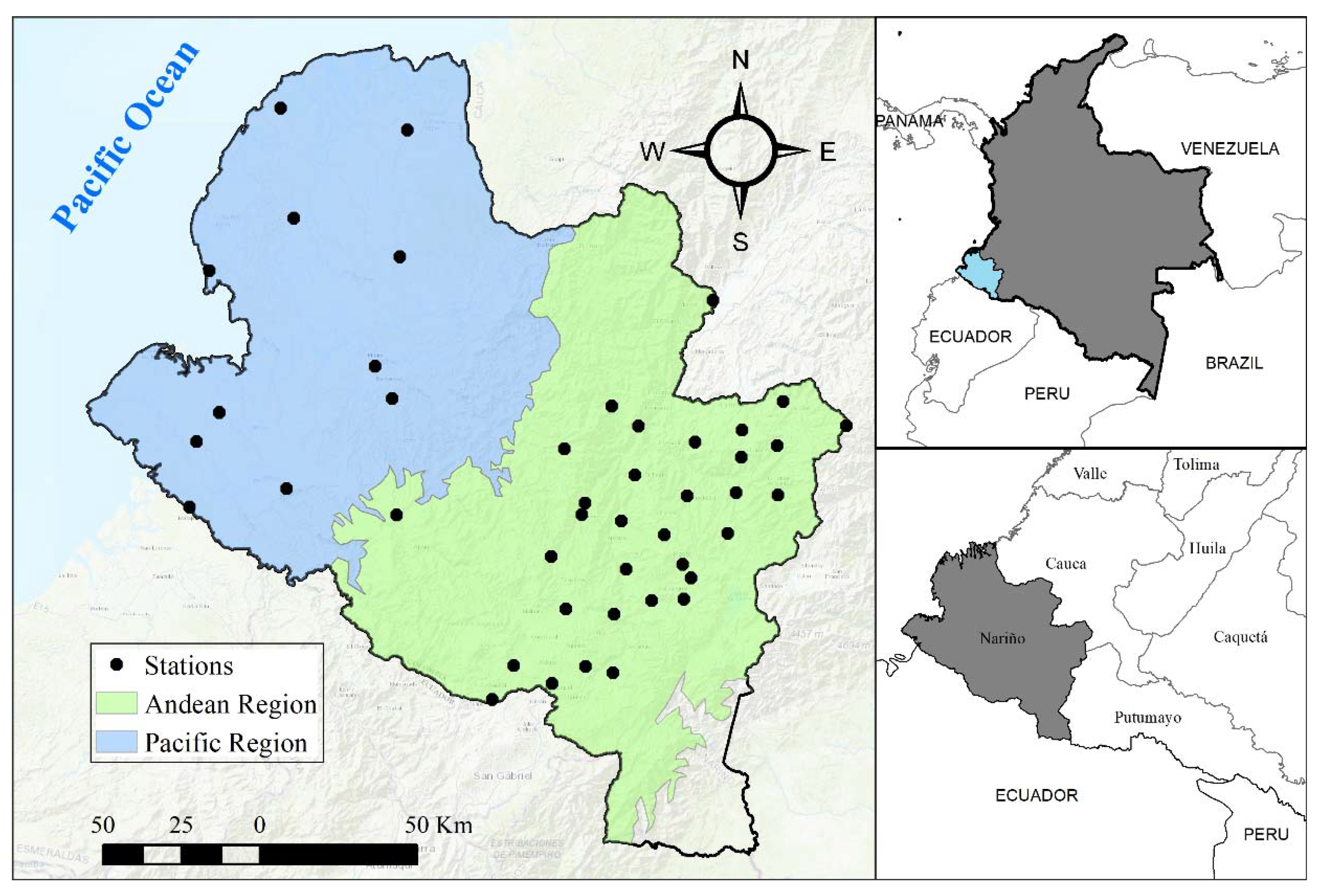
2.1. Study Area

The Department of Nariño is located in Southwestern Colombia, in the south of the Colombian Biogeographic Choco, which is considered a biodiversity hotspot in the world (Figure 1). This region lies near the Tropical Pacific Ocean and is crossed in the middle by the Andes Mountain Range [39]. The study area has two climatic sub-regions: the AR and the PR that cover an approximate surface area of 15,466 km² and 14,754 km², respectively [35].

These sub-regions have different rainfall regimes. The rainfall in AR records a bimodal annual cycle (Figure 2a) [35], with an average monthly rainfall of 130 mm/month⁻¹. Otherwise, PR depicts a unimodal annual cycle (Figure 2b), with an average monthly rainfall of 350 mm/month⁻¹.

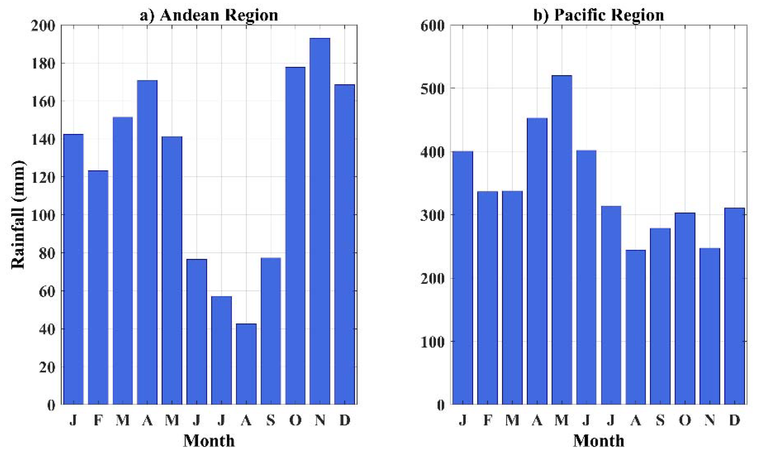
2.2. Rainfall Data

We used a monthly rainfall time-series from 1983 to 2016 of forty-four rainfall gauge stations distributed over Nariño, provided by Instituto de Hidrología, Meterología y Estudios Ambientales (IDEAM) of Colombia. Thirty-three (33) and eleven (11) gauge stations belong to the AR and PR, respectively. The missing data in the time series were less than 11% and were estimated using the Non-linear Principal Component Analysis (NLPCA) through the methodology suggested by Scholz et al. [40]. Details about the estimation of missing data are available in Canchala et al. [39].

2.3. Large-Scale Climate Indices

Eight large-scale climate indices linked to the SST in the Tropical Pacific Ocean and ENSO phenomenon were used as exogenous variables (predictor variables). Several studies performed in Western Colombia evidenced that its hydroclimatology has high concurrent or lagged correlations with these large-scale climate indices [24,25,26,27,28,30,31,33,34,35,41,42]. Therefore, we use regional Sea Surface Temperatures (SSTs): SST1+2 (0°–10° S, 90°–80° W), SST3 (5° S–5° N, 90°–150° W), SST3.4 (5° N–5° S, 170°–120° W), and SST4 (5° N–5° S, 160° E–150° W) provided by the National Oceanic and Atmospheric Administration (NOAA) and available at https://www.esrl.noaa.gov/psd/data/climateindices/list/ [43]. We also selected other indices: ONI, calculated as the three-month moving average of SST anomalies in the Niño3.4 region [44]; MEI, corresponding to the linear combination of six variables from the tropical Pacific Ocean [45]; SOI, characterized by the anomalies of the sea level pressure between Darwin and Tahiti; and the PDO index, linked with the SST anomalies in the North Pacific Ocean. The ONI, MEI, and SOI indices were obtained from the NOAA website, while the PDO index was obtained from the Joint Institute for the Study of the Atmosphere and Ocean (http://research.jisao.washington.edu/pdo/). All these indices are the exogenous variables on a monthly scale analogous to the rainfall dataset for the 1983–2016 period.

In addition, we changed the monthly rainfall values into anomalies by subtracting the mean monthly climatological value to each month from the monthly values to eliminate the annual cycle.

3. Methodology

The overall methodology applied in this research project is based on three ANNs approaches Non-linear Principal Component Analysis (NLPCA), Neural Network Autoregressive Moving Average with eXogenous variables (NNARMAX), and Inverse NLPCA. The forecasting scheme uses time lags between the exogenous variables and the predictand variable (rainfall anomalies); the flowchart of the methodology is shown in Figure 3. Initially, we used the NLPCA approach to reduce the dimensions of the monthly rainfall anomalies of a region ($x_n$) and to extract the main information of the datasets. The Non-linear Principal Components (NLPCs) obtained in the bottleneck of the NLPCA approach ($y_m$) depict the main modes of rainfall anomalies variability in each region (AR and PR). Subsequently, each estimated NLPC for one region was forecasted through the NNARMAX model $\left(y_m{}^{\prime }\right)$. Here, we used as exogenous variables the large-scale climate indices that have a significant lagged correlation with the estimated NLPCs for each region. Thereafter, the forecasted NLPCs $\left(y_m{}^{\prime }\right)$ were used as input variables in the Inverse NLPCA approach to obtain the monthly rainfall anomalies $\left({\overline{x}}_n{}^{\prime }\right)$ forecasted for each region. Finally, we use three performance metrics to evaluate both forecasting models.

The monthly NLPCs data and climate indices were used to build and validate the non-linear NNARMAX model. We divided the dataset from 1983 to 2014 into three sub-sets: 40% for the training of the ANN architecture, 30% for the validation phase, and 30% for the test phase; we randomly selected all indices at the sets to avoid overfitting and underfitting. Data from the two last years, i.e., from 2015 to 2016, were used to assess the performance of the forecasting model.

3.1. Non-Linear Principal Component Analysis

In this study, NLPCA was used to establish dominant modes of variability of monthly rainfall anomalies in AR and PR. NLPCA is a non-linear generalization of principal component analysis [46] that allows extracting non-linear components with the least loss of information, including lines and curves. Therefore, NLPCA generalizes the principal components from straight lines to curves, describing the inherent structure of the data by curved spaces, allowing better data space coverage and representation [47]. For this purpose, the ANN activate the first part of network that represents the extraction function ${\mathsf{\Phi }}_{extr}: x\to y$. This method was developed by Hsieh [46] and Scholz [47], using the multi-layer perceptron of an auto-associative topology, which is better known as an auto-encoder or bottleneck.

In the last decades, non-linear methods have been widely applied to analyze oceanographic, meteorological, and hydroclimatological datasets [35,39,46,48,49,50,51,52,53], considering that most of the atmosphere–climate relationships are not linear. We used the NLPCA toolbox provided by Scholz. [47] (available in http://www.nlpca.org/matlab.html) to get the hierarchically ordered features by training sequentially and calculating the explained variance of each NLPC. In this study, the NLPCA training was performed with the dataset from 1983 to 2014, which corresponds to the calibration period of the NNARMAX model. Once the NLPCA was trained, we used this trained network to estimate the values of the last two years (2015–2016), considering the ability of generalization that this approach has. The estimation of this period will allow us to corroborate the forecasting results obtained by the NNARMAX model in the following step. Furthermore, we selected the best architecture taking into account the best performance in terms of the highest percentage of explained variance.

3.2. Selecting of Significant Predictors

The relationships between NLPCs for AR and PR and large-scale climate indices described in Section 2.3 were evaluated using Pearson correlations and the Student t-test to assess the statistical significance with a confidence value of 99% ($\alpha =0.01)$, corresponding to r > 0.128. Furthermore, we used partial cross-correlations to measure the degree of correlation of the teleconnections and its persistence by calculating lagged correlation coefficients (r) for a range from 0 to 12 months, considering that the large-scale climate indices precede the monthly rainfall. The lagged climatic indices from 6 to 12 months with r > 0.128 were selected as rainfall anomalies predictors (Figure 4).

3.3. Building a Model Using Artificial Neural Network

ANN is a data-driven mathematical model that emulates a human brain neural network, which has been used to solve issues such as forecasting and classification [54]. There are different architectures of ANN; however, the most common model is a Multi-Layer Perceptron (MLP) neural network, which has a structure with an input layer, single or multiple hidden layers, and an output layer. The MLP has been widely used to forecast several phenomena in meteorology and hydroclimatology [3,9,17,54,55,56,57]. The typical mathematical expression of the ANN is:

$$y_k=f_0\left[{\displaystyle \sum }_{j=1}^n{w}_{kj}{f}_h\left({\displaystyle \sum }_{j=1}^m{w}_{ji}{x}_i+w_{jb}\right)+w_{kb}\right]$$

(1)

where $y_k$ is the output, for time t; $x_i$ is the $i$th input; $w_{ji}$ are the synaptic weights connecting the input layer and the hidden layer; $w_{kj}$ are the synaptic weights connecting the neurons of the hidden and output layers; $f_0$ and $f_h$ are the activation functions in the output and the hidden layers, respectively; $n$ and $m$ are the number of output and hidden layers, respectively, and $w_{jb}$ and $w_{kb}$ are the bias for the hidden and output layers [15,54].

For training the networks, we use a learning algorithm to find the best combination of synapse weights with the least error [17] that were estimated using the back-propagation algorithm, which propagates back the error between the actual output and the calculated output through the network to update the parameters. The mathematical expression is described in Equation (2), as follows:

$$E={\displaystyle \sum }_{p=1}^P{E}_p={\displaystyle \sum }_{p=1}^P{\displaystyle \sum }_{k=1}^n{\left(y_{pk}-{\widehat{y}}_{pk}\right)}^2$$

(2)

where $E$ is the total error, $P$ is the number of input sets, and $E_p$ is the error of the squared difference between the actual outputs $y_{pk}$ and the forecasted outputs ${\widehat{y}}_{pk}$ for pattern $p$ [15].

3.3.1. NNARMAX Model

For the forecasting of the NLPCs for AR and PR, we built specifically an NNARMAX model, which allows showing and characterizing complex non-linear relationships between the main modes of variability of rainfall anomalies and large-scale climate indices depicting how an output signal (response variable) is related to a number of input signals (explanatory variables) and their combined interlinkage [58].

We considered many exogenous variables; therefore, the NNARMAX model is described in Equation (3) as follows:

$$\begin{array}{c}y\left(k+1\right)=f(y\left(k\right), y\left(k-1\right),\cdots ,y\left(k-n_y\right), u_1\left(k\right), u_1\left(k-1\right), \cdots ,\\ u_1\left(k-n_{u1}\right), \cdots ,u_2\left(k\right), u_2\left(k-1\right),\cdots ,u_2\left(k-n_{u2}\right)\cdots ,\\ u_r\left(k\right),u_r\left(k-1\right),\cdots ,u_r\left(k-n_{ur}\right),e\left(k\right),e\left(k-1\right),\cdots ,e\left(k-n_e\right))\end{array}$$

(3)

where $y\left(k+1\right)$ is the output; $n_y$ are the lags of output; $u_x\left(k\right)$ are the input variables (exogenous terms) with $x\in \left[1,r\right]$; $n_{ux}$ are the lags of the exogenous terms; $k$ is the sample time; $e\left(k\right)$ is a noise sequence; $n_u\ge 0$ is the maximum lags; and $f$ is a non-linear function. $e\left(k\right)=y\left(k\right)-\widehat{y}\left(k\right)$, where $\widehat{y}\left(k\right)$ is the forecasted value at time instant $k$, and $n_e$ are the lags of the respective differences of $e\left(k\right)$.

The NNARMAX model was trained as an MLP neural network, using the Bayesian regularization and the back-propagation algorithm to update the weight and bias values. We used the non-linear hyperbolic tangent and linear functions for the hidden and output layers activation, respectively. Furthermore, the network training phase is performed in an open loop, while the validation phase is performed in a closed loop assuming a moving average equal to zero, so the forecasting depends only on the number of lags of the exogenous variables.

The number of neurons in the hidden layer was estimated through a trial and error approach, which is a method that is widely used given that there is no standard methodology for its estimation [3]. Therefore, in the present study, the best number of hidden neurons for the model was determined through the correlation coefficient (r) that measures the relationship between the predicted value and the observed value. Thus, the model was trained with different numbers of hidden neurons, and the number of neurons that provided the highest r value was selected. Finally, to avoid over-fitting in the NNARMAX model, we implemented an early stopping technique in which the training stops when the errors during the validation phase start to increase, even when the errors in the training phase decrease.

3.3.2. Backward Elimination Method

Given that in NNARMAX we can use as exogenous variables all the predictors that meet the condition described in Section 3.2, we use the backward elimination method [59] for the predictor variable selection of the Simplified-NNARMAX model. This method starts with the training of the model, considering all possible input predictors. From the selected input predictors, the least significant predictors are removed until the main predictors remain; this method is an iterative procedure that allows for improving the performance of the model [60]. The fewer exogenous variables the model has, the more robust it is, given that the prediction depends on less external information, in this case, on fewer macroclimatic indices. The simplified model outputs are the inputs for the Inverse NLPCA.

3.4. Inverse NLPCA

The inverse NLPCA is the second step of the NLPCA full approach; this uses the reconstruction function ${\mathsf{\Phi }}_{gen}: y\to {\overline{x}}_n{}^{\prime },$ which is performed by a feed-forward network. Equation (4) shows that the output ${\overline{x}}_n{}^{\prime }$ is dependent upon the input $y$ and the ANN synaptic weights $wϵW_3,W_4$.

$${\overline{x}}_n{}^{\prime }={\mathsf{\Phi }}_{gen}\left(w,y\right)=W_{4}g \left(W_{3}y\right)$$

(4)

where ${\mathsf{\Phi }}_{gen}$ reconstructs the dataset $\overline{x}{}^{\prime }$, which should be close to the target dataset $x$ by minimizing the squared error ${\Vert x-\overline{x}{}^{\prime }\Vert }^2$. More information about this process is widely detailed in Scholz et al. [40,61]. In this regard, we reconstructed the rainfall anomalies forecasted of AR and PR, using the inputs of the forecasted NLPCs obtained through the Simplified-NNARMAX.

3.5. Forecast Verification

To evaluate the model performance and the forecast skill in both training and testing timestamps, we used three statistical methods: Root Mean Square Error (RMSE), Mean Absolute Error (MAE), and Pearson correlation coefficients (r) [62], applying Equations (5)–(7), respectively.

$$\mathrm{RMSE}=\sqrt{ \frac{{{\displaystyle \sum }}_{i=1}^n{\left(F_i -O_i\right)}^2}{n}}$$

(5)

$$\mathrm{MAE}=\frac{1}{n} {\displaystyle \sum }_{i=1}^n\left|F_i-O_i\right|$$

(6)

$$\mathrm{r}=\frac{\frac{1}{n}\left({{\displaystyle \sum }}_{i=1}^n\left(P_i-{\overline{F}}_t\right)-\left(O_i-{\overline{O}}_t\right)\right)}{\sqrt{{{\displaystyle \sum }}_{i=1}^n{\left(F_i-{\overline{F}}_t\right)}^2 } \sqrt{{{\displaystyle \sum }}_{i=1}^n{\left(O_i-{\overline{O}}_t\right)}^2}}$$

(7)

where $O_i$ and $F_i$ are the observed and forecasted value, respectively, $n$ corresponds to the number of all observations, and ${\overline{O}}_t$ and ${\overline{F}}_t$ are the mean of the observed and forecasted values, respectively.

4. Results and Discussion

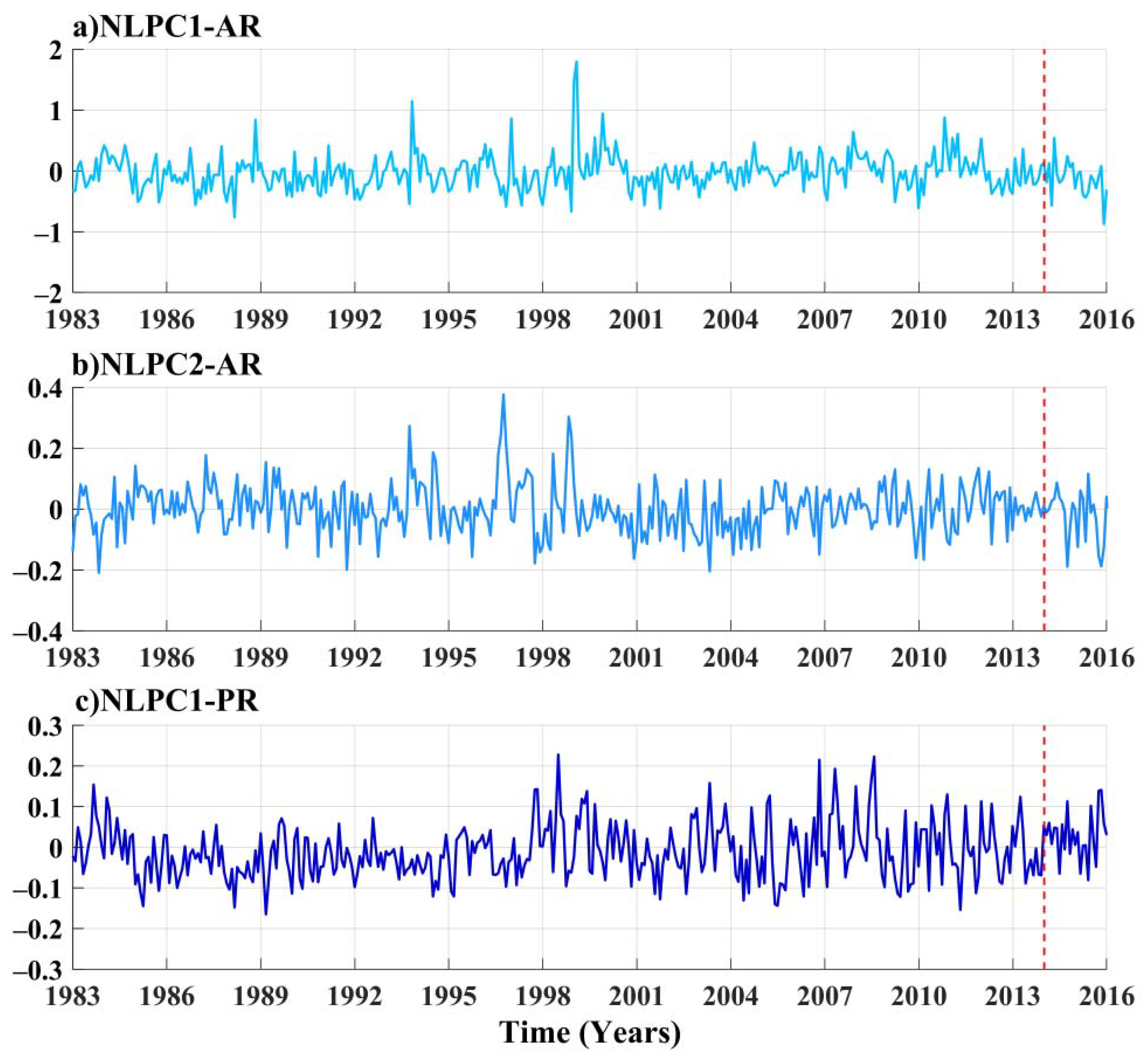
4.1. Modes of Monthly Rainfall Anomalies Variability

Using NLPCA, we established the main modes of monthly rainfall anomalies variability for the sub-regions AR and PR. The NLPCA for AR (PR) results showed two (one) significant NLPCs that explained around 73% (48%) of the original dataset variance. We assess several topologies to define which is the best in terms of the highest explained variance. The best topologies for each region are shown in

Table 1. Topologies and explained variance for the Andean Region (AR) and the Pacific Region (PR) using the NLPCA approach.

Region	Topologies	Explained Variance (%)
		NLPC1	NLPC2	Total
AR	33-25-15-2-15-25-33	55.26	17.46	72.72
PR	11-8-5-1-5-8-11	47.51	–	47.51

; the best result for AR was found with a [33-25-15-2-15-25-33] network topology, whereas the best outcome for PR was found with a [11-8-5-1-5-8-11] network topology. The components were estimated in hierarchical order.

The time-series for each NLPC for AR (NLPC1-AR and NLPC2-AR) and PR (NLPC1-PR) are shown in Figure 5. The main negative (positive) values for the NLPC1-AR (Figure 5a) include periods of 1987–1988, 1997–1998, 2009–2010, and 2015–2016 (1988–1989, 1999–2001, 2008–2009, 2010–2011, and 2011–2012); NLPC2-AR (Figure 5b) recorded negative (positive) values in the periods 1991–1992, 1997–1998, 2002–2003, 2009–2010, and 2015–2016 (1985–1986, 1988–1989, 1998–1999, and 2011–2012). The negative (positive) periods highlighted in NLPC1-AR and NLPC2-AR correspond to the EN (LN) events [43,63]. Meanwhile, NLPC1-PR (Figure 5c) recorded positive (negative) values during 1997–1998 and 2015–2016 (1985–1986, 1988–1989, and 2011–2012), which match with EN (LN) events. An extensive discussion on the relationship between the main components obtained and the period’s EN and LN recorded in the region is available in Canchala et al. [35].

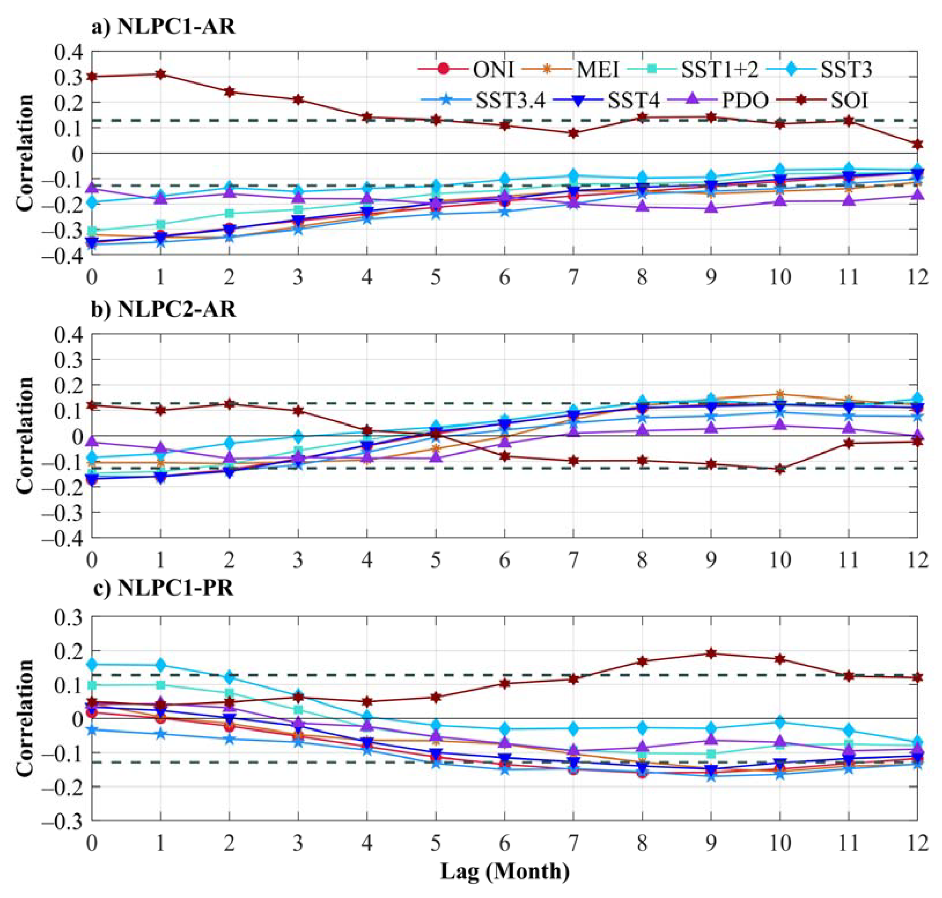
4.2. Identification of Significant Exogenous Variables

The partial cross-correlations between NLPC1-AR, NLPC2-AR, and NLPC1-PR and the eight possible predictors described in Section 2.3 are presented in Figure 6a–c, respectively. We observe that statistically significant positive (negative) cross-correlations (r >$\pm$0.128) at lag=0 occur between NLPC1-AR and SOI (SST1+2, SST3, SST3.4, SST4, ONI, MEI, and PDO), evidencing that between the variables, there exists a direct (inverse) physical relationship. For some variables such as SST1+2, SST3.4, SST4, MEI, SOI, and PDO, the relationship is persistent and statistically significant until lags 6, 10, 8, 9, 11, and 12, respectively, with the strongest correlations in the SST3.4, PDO, and MEI indices (See Figure 6a). For NLPC2-AR, we observed the negative synchronous correlations and statistical significance with SST3.4, SST4, and ONI; however, in lags greater than 8 months, we identified significant positive correlations with SST1+2, SST3, MEI, and SOI (See Figure 6b).

In contrast, the partial cross-correlations between NLPC1-PR and the eight climate indices (Figure 6c) showed that at lag = 0, there are positive correlations that are statistically significant only with the SST3 index. However, in lags greater than 5 months, negative cross-correlations that were statistically significant with SST3.4, SST4, MEI, SOI, and ONI indices were observed, with the strongest correlations in the SST3.4, SOI, and MEI indices. A noticeable aspect of partial cross-correlations for NLPC2-AR and NLPC2-PR is the fact that the correlations change the sign in the time-lagged. This condition also was evidenced by Córdoba-Machado et al. [64]. They reported the change of sign of the correlations between seasonal rainfall in Colombia and the SST patterns with several season lags, which is a condition linked to the periodicity of the variability of the ENSO phenomenon.

Overall, the results obtained showed that the teleconnections between monthly rainfall and ENSO climate indices are stronger and more persistent in the AR than the PR. The outcomes for AR are consistent with the results found by Navarro et al. [65], Montealegre [66], Córdoba-Machado et al. [64] (AR of Colombia), Campozano et al. [67], and Morán-Tejeda et al. [68] (AR of the neighboring country Ecuador). They showed an increase (decrease) in the rainfall values linked to negative (positive) anomalies of the SST in the central region of the Tropical Pacific Ocean. Regarding the persistence of the influence of the ENSO indices on the rainfall, the results are consistent with those of Navarro et al. [65] and Canchala et al. [34]. They reported a persistent lagged influence of up 9 and 10 months, mainly with the SST in the central region of the Tropical Pacific Ocean.

Furthermore, the results for AR showed that the PDO index has high and persistent correlations with the rainfall in this region. Although PDO is a phenomenon that occurs in the Pacific Ocean north of 20° N that modulates warm and cold phases at an interdecadal time scale, it can influence the climatic variability in some regions of South America. According to Garreaud et al. [69], whether the PDO is in its cold (negative index) or warm (positive index) stage, the effects of ENSO on rainfall can decrease or increase. When ENSO and PDO are in phase, the dry (wet) anomalies led by EN (LN) intensify over the regions influenced by a typical ENSO event (canonical regions). In contrast, if ENSO and PDO are out of phase, the dry or wet anomalies vanish [70]. Therefore, in AR high (low), rainfall is favored when negative LN/PDO (positive EN/PDO) episodes occur.

Concerning the results obtained for rainfall in PR, we observed that the cross-correlations with the SST1+2 and SST3 indices were positive until lags 3 and 4, respectively. Subsequently, the value sign changed, whereas the cross-correlations with the SST3.4 index were negative in all the delays evaluated. The positive relationship with the SST1+2 index indicated that the positive (negative) rainfall anomalies in PR were weakly linked with the positive (negative) anomalies in SST of the east of the Tropical Pacific Ocean. In contrast, the correlations with the SST3+4 and SST4 indices were negative and statistically significant from six and eight lags, respectively. In regard to the opposite influence exerted by the SST in the east and central region over the rainfall in PR, several studies had reported that two kinds of El Niño drive to different effects on rainfall variability from the regional to global scale [71,72]. The El Niño Canonical (ENC), which is characterized by positive or negative SST anomalies in the east of the Tropical Pacific Ocean, and the El Niño Modoki (ENM), which is characterized by positive SST anomalies in the Central Pacific Ocean, which is bounded by negative SST anomalies in the eastern and western Tropical Pacific Ocean [73].

Here, we found a contrary influence exerted by the SST in the east and central regions over the rainfall in PR, which seems to suggest that the ENM mostly modulates the rainfall in PR, more than the ENC. This suggestion is consistent with the findings reported by Córdoba-Machado et al. [71]. They found that the rainfall in some regions of Colombia is greater during ENM than during ENC, such as the Pacific Coast of the department of Nariño. Here, they found that gauge stations with data significantly correlated with ENM, but not with ENC, concluding that this sub-region seems to show a particular sensitivity to the ENM conditions. Furthermore, they found that ENM exerts an opposite influence to the one exerted by ENC.

From the previous analysis, we selected predictors with statistically significant correlations in lags from 6 until 12 months (6 $\le$ lags $\le$ 12), considering that these indices have a persistent relationship with the monthly rainfall anomalies in AR and PR. The strong correlations at lags higher than 5 months make them potential predictors of rainfall, given that the large lag time allows developing early warning systems for the several socio-economic sectors and decision-makers [53]. The exogenous variables and the respective lags selected for the preliminary NNARMAX model for NLPC1-AR, NLPC2-AR, and NLPC1-PR are shown with shading in

Table 2. Exogenous variables selected as predictors in the preliminary Neural Network Autoregressive Moving Average with eXogenous variables (NNARMAX) model for NLPC1-AR, NLPC2-AR, and NLPC1-PR.

NLPCs	Climate Index	Preliminary NNARMAX Model
		Lags
		6	7	8	9	10	11	12
NLPC1-AR	SST1+2	−0.147	−0.121	−0.121	−0.113	−0.083	−0.081	−0.075
	STT3.4	−0.231	−0.197	−0.164	−0.153	−0.137	−0.120	−0.102
	SST4	−0.182	−0.148	−0.134	−0.124	−0.103	−0.089	−0.079
	MEI	−0.166	−0.148	−0.149	−0.163	−0.155	−0.136	−0.115
	ONI	−0.189	−0.169	−0.151	−0.131	−0.112	−0.094	−0.078
	SOI	0.109	0.078	0.139	0.141	0.115	0.126	0.034
	PDO	−0.172	−0.198	−0.213	−0.218	−0.191	−0.190	−0.168
NLPC2-AR	SST1+2	0.061	0.097	0.129	0.133	0.126	0.118	0.132
	SST3	0.058	0.097	0.132	0.140	0.122	0.119	0.145
	MEI	−0.004	0.064	0.118	0.145	0.162	0.140	0.122
NLPC1-PR	STT3.4	−0.150	−0.147	−0.156	−0.170	−0.164	−0.147	−0.133
	SST4	−0.115	−0.126	−0.139	−0.148	−0.129	−0.117	−0.110
	MEI	−0.075	−0.104	−0.127	−0.146	−0.155	−0.139	−0.134
	ONI	−0.134	−0.149	−0.159	−0.158	−0.148	−0.131	−0.117
	SOI	0.103	0.116	0.168	0.192	0.175	0.125	0.121

The shading lags indicate a significance level of 0.01 is $\pm$ 0.128.

.

The outcomes showed in Table 2 are consistent with the results obtained in earlier research in Colombia that suggests that the forecasting of the hydroclimatology variables based on ENSO indices is possible. According to Gutierrez et al. [74], the streamflows of some Colombian rivers can be forecasted in particular with the MEI, SOI, and SST4, given that they found strong correlations for lags between 4 and 6 months. Regarding the rainfalls, Poveda et al. [41] suggested that ENSO indices, mainly SST3 and SST4, can become relevant to forecast the seasonal rainfall over the Andes region, considering the high correlations registered with the rainfall in the tropical Andes. In the neighboring country of Ecuador, a country with similar topographic conditions of Nariño, Vicente-Serrano et al. [75] concluded that the SST3.4 index explains the drought variability in the Andes Mountains range. Moreover, Cordoba Machado et al. [64] registered that the seasonal rainfall in Colombia can be predicted using the ENC and ENM, since the ENC is the most important pattern for explaining the seasonal rainfall in the country, and ENM is the second pattern that influences the rainfall.

According to Serrano et al. [75] and Cordoba Machado et al. [71], the differences found in the response patterns to the ENSO phenomenon in sub-regions that are close to each other are given by the strong orography complexity that modulates the influence of atmospheric circulation processes in the region and alters the ENSO effects over the northwest of South America.

4.3. Preliminary NNARMAX Model for Rainfall Forecasting

The optimal preliminary NNARMAX models frame, with the selected exogenous variables (see Table 2) for NLPC1-AR, NLPC2-AR, and NLPC1-PR was established, varying the number of hidden neurons from 12 to 20. For each topology, i.e., an MLP with a defined number of hidden neurons, we ran it fifty times for both training and validation tests. The best networks were saved and evaluated for testing. For each study, the optimal number of hidden neurons was found to be 12 (NLPC1-AR), 20 (NLPC2-AR), and 18 (NLPC1-PR). The performance of the preliminary NNARMAX models was tested using Pearson’s correlation coefficients. For the NNARMAX training, the dataset from 1983 to 2014 was used for the knowledge of the input variables patterns; the output data from the training are called in this study calibration. The dataset from 2015 to 2016 was used to test the preliminary NNARMAX model, and the results were considered as the testing period. The comparisons of the NLPCs observed with the NLPCs trained in the calibration period and the forecasted NLPCs in the testing phase are shown in Figure 7. In general, the NNARMAX models forecasting for NLPC1-AR (r = 0.99) (Figure 7a) and NLPC1-PR (r = 0.99) (Figure 7c) are more accurate than the NLPC2-AR model (r = 0.97) (Figure 7b); however, all the NNARMAX models capture the positive and negative peaks of the time-series; these results support the accuracy of the non-linear proposed models.

4.4. Simplified NNARMAX Model

Given that the preliminary NNARMAX models have exogenous variables, all possible input predictors can even be correlated with each other, being redundant. Therefore, we use the backward elimination method to remove predictors and establish the Simplified-NNARMAX models for the NLPCs studied, and finally, we use this forecasted NLPCs as input in the inverse NLPCA model for the reconstruction of the forecasted rainfall anomalies. The exogenous variables and the respective lags for the Simplified-NNARMAX model for NLPC1-AR, NLPC2-AR, and NLPC1-PR are shown with shading in

Table 3. Exogenous variables selected as predictors in the Simplified-NNARMAX Model for NLPC1-AR, NLPC2-AR, and NLPC1-PR.

NLPCs	Climate Indices	Simplified-NNARMAX Model
		Lags
		6	7	8	9	10	11	12
NLPC1-AR	STT3.4	−0.231	−0.197	−0.164	−0.153	−0.137	−0.120	−0.102
	MEI	−0.166	−0.148	−0.149	−0.163	−0.155	−0.136	−0.115
	PDO	−0.172	−0.198	−0.213	−0.218	−0.191	−0.190	−0.168
NLPC2-AR	SST1+2	0.061	0.097	0.129	0.133	0.126	0.118	0.132
	SST3	0.058	0.097	0.132	0.140	0.122	0.119	0.145
	MEI	−0.004	0.064	0.118	0.145	0.162	0.140	0.122
NLPC1-PR	STT3.4	−0.150	−0.147	−0.156	−0.170	−0.164	−0.147	−0.133
	MEI	−0.075	−0.104	−0.127	−0.146	−0.155	−0.139	−0.134

The shading lags indicate a significance level of 0.01 ($\pm$ 0.128).

, and the simplified models developed for each one are given in Equations (8)–(10), respectively.

$$y_1\left(k+1\right)=f\left(\begin{array}{c}{y}_1\left(k\right),y_1\left(k-1\right),y_1\left(k-2\right),x_1\left(k-6\right),x_1\left(k-7\right),x_1\left(k-8\right),x_1\left(k-9\right),\\ x_1\left(k-10\right),x_2\left(k-6\right),x_2\left(k-7\right),x_2\left(k-8\right),x_2\left(k-9\right),x_2\left(k-10\right),\\ x_2\left(k-11\right),x_3 \left(k-6\right),x_3 \left(k-8\right),x_3 \left(k-9\right),x_3 \left(k-10\right),x_3 \left(k-11\right),\\ x_3\left(k-12\right),e\left(k\right), e\left(k-1\right), e\left(k-2\right)\end{array}\right)$$

(8)

$$y_2\left(k+1\right)=f\left(\begin{array}{c}{y}_2\left(k\right),y_2\left(k-1\right),y_2\left(k-2\right),x_4 \left(k-8\right),x_4 \left(k-9\right),x_4 \left(k-12\right),\\ x_5\left(k-8\right),x_5\left(k-9\right),x_5\left(k-12\right),x_2\left(k-9\right),x_2\left(k-10\right),\\ x_2\left(k-11\right),e\left(k\right), e\left(k-1 \right), e\left(k-2 \right) \end{array}\right)$$

(9)

$$y_3\left(k+1\right)=f\left(\begin{array}{c}{y}_3\left(k\right),y_3\left(k-1\right),y_3\left(k-2\right),x_1\left(k-6\right),x_1\left(k-7\right),x_1\left(k-8\right),\\ x_1\left(k-9\right),x_1\left(k-10\right),x_1\left(k-11\right),x_1\left(k-12\right),x_2\left(k-9\right),\\ x_2\left(k-10\right), x_2\left(k-11\right),x_2\left(k-12\right), e\left(k\right), e\left(k-1\right), e\left(k-2\right)\end{array}\right)$$

(10)

where $y_1\left(k+1\right)$, $y_2\left(k+1\right)$, and $y_3\left(k+1\right)$ are the forecasted outputs $NLPC1-AR$, $NLPC2-AR$, and $NLPC1-PR$, in closed loop, respectively; $u_x\left(k\right)$ are the input variables (exogenous variables);$u_1=$ SST3.4, $u_2=$ MEI, $u_3=$ PDO, $u_4=$ SST1+2, and $u_5=$ SST3; $k$ is the sample time; $e\left(k\right)$ is a noise sequence.

The optimal Simplified-NNARMAX models structure with the selected exogenous variables for NLPC1-AR, NLPC2-AR, and NLPC1-PR was established by varying the number of hidden neurons from 12 to 24 with a similar methodology to the one used for preliminary NNARMAX. Now, the optimal number of hidden neurons was 16, 20, and 22 for NLPC1-AR, NLPC2-AR, and NLPC1-PR, respectively. Again, the performance of the Simplified-NNARMAX models for the calibration and testing period used Pearson’s correlation coefficients for evaluation. The comparisons of the NLPCs observed with the NLPCs trained in the calibration period and the forecasted NLPCs in the testing phase are shown in Figure 8.

The Simplified-NNARMAX models have fewer exogenous input variables than the preliminary NNARMAX models shown in Figure 7; however, the Pearson’s correlation result remained at 0.99, 0.97, and 0.99 for NLPC1-AR (Figure 8a), NLPC2-AR (Figure 8b), and NLPC1-PR (Figure 8c), respectively. The accuracy of forecasting using Simplified-NNARMAX was similar to that obtained in the forecasting using preliminary-NNARMAX, with the advantage that these models depend only on two or three exogenous variables, which makes them more independent models compared to the preliminary NNARMAX models. The exogenous variables for Simplified-NNARMAX for NLPC2-AR remained the same as the initial one, since the elimination of a variable affected the forecasting performance.

Overall, the results demonstrate the ability of the large-scale climate indices chosen in this study to predict the main modes of monthly rainfall anomalies of the AR and PR in the Department of Nariño. The results also highlight that the monthly rainfall variability in these sub-regions is strongly linked with the ENSO phenomenon; also, it needs to be posited that its influence is not only synchronous but also remains in time up to 12 months in some cases.

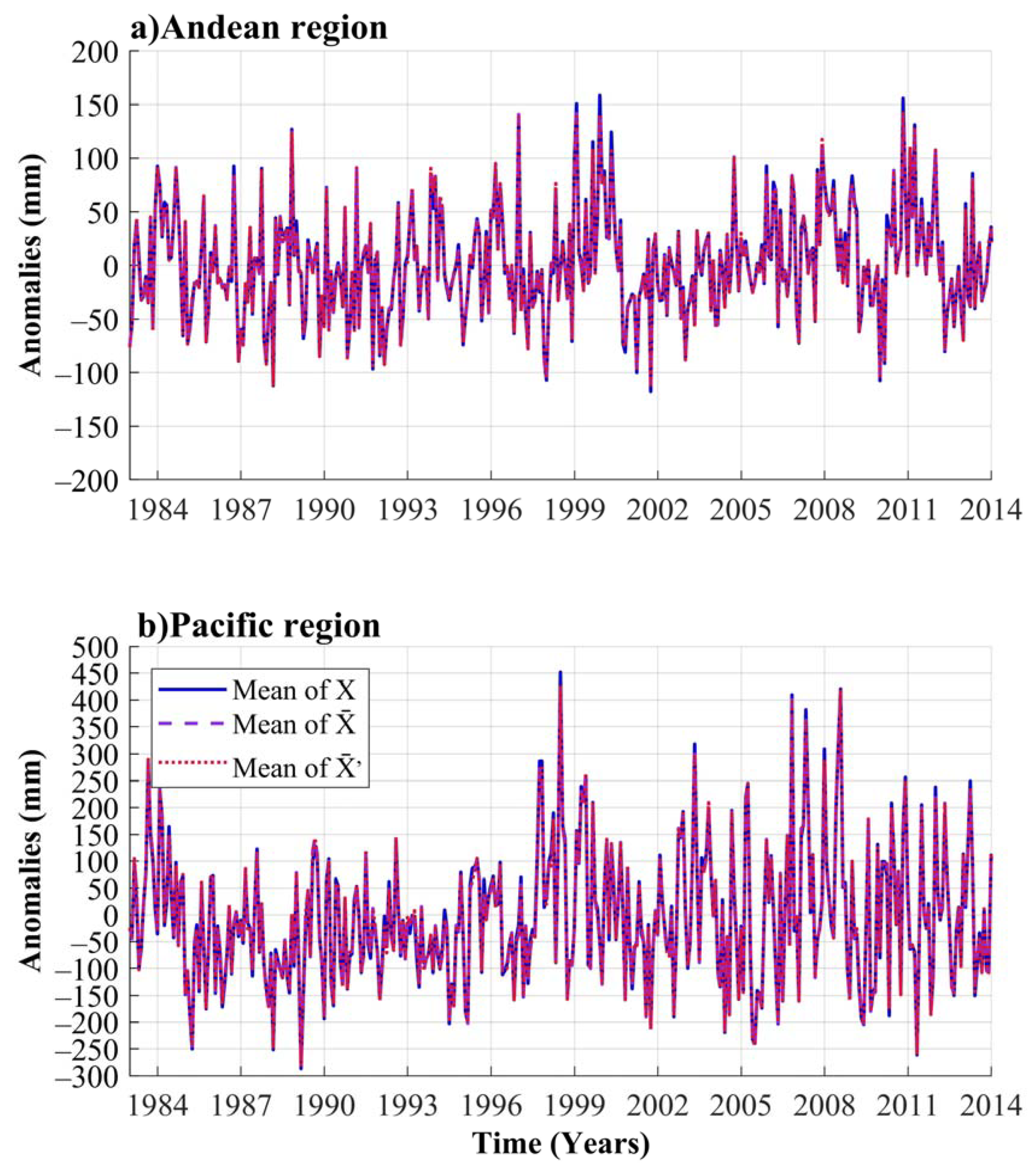
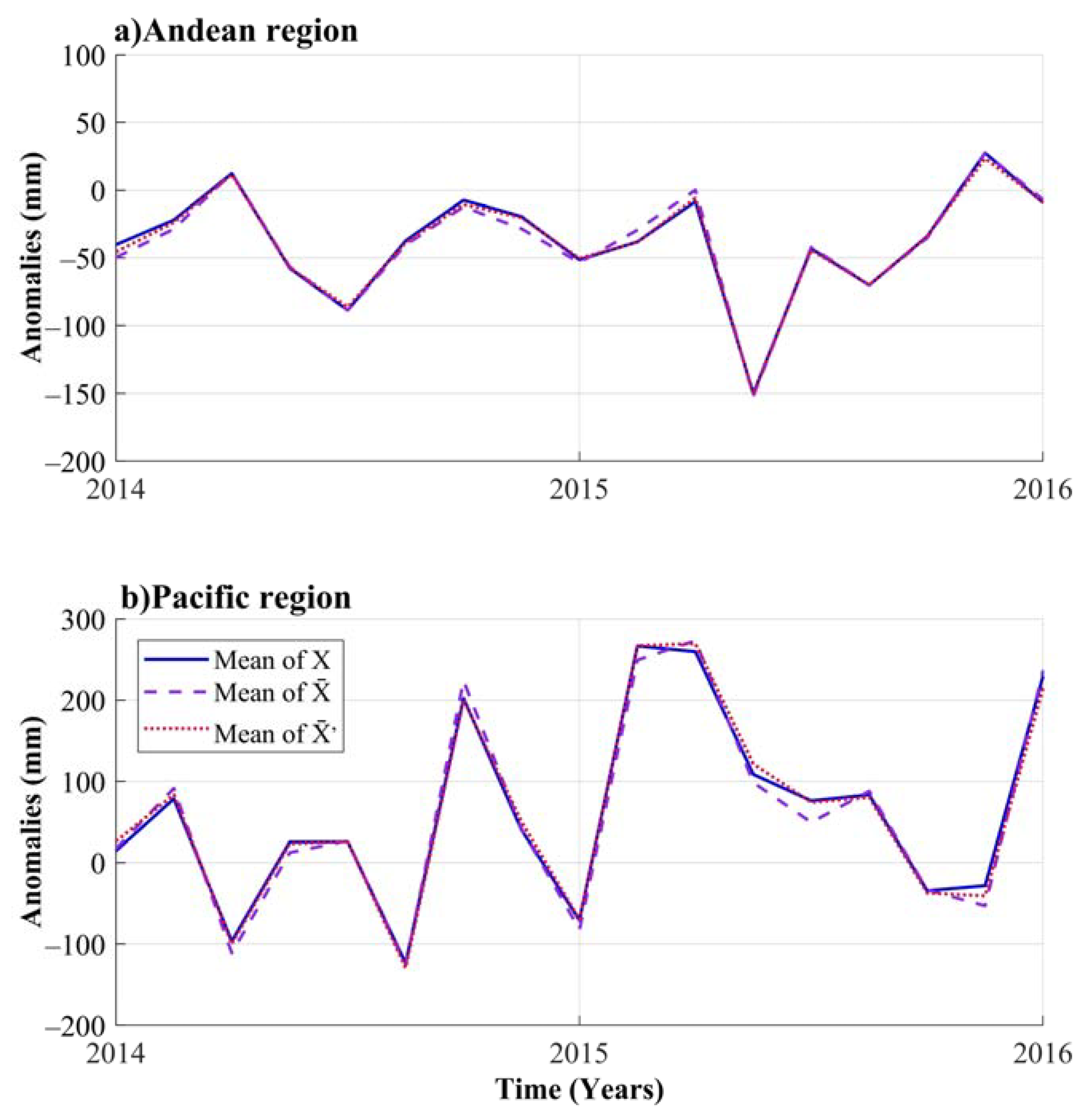
4.5. Inverse NLPCA Approach

In this section, we show the ability of the Inverse NLPCA approach to reconstruct the mean of forecasted monthly rainfall anomalies of AR (PR), using the outputs obtained of the Simplified-NNARMAX for NLPC1-AR and NLPC2-AR (NLPC1-PR) as inputs. Figure 9a,b depicts the observed rainfall anomalies time series $\left(X\right)$, the reconstructed rainfall anomalies times series without using NLPCs forecasted $\left(\overline{X}\right)$, and the forecasted monthly rainfall anomalies $\left(\overline{X}{}^{\prime }\right)$ during the calibration period for AR and PR, respectively. The reconstruction of this time series for the testing period for AR and PR are reported in Figure 10a,b, respectively. The performance metrics for calibration and testing phases are shown in

Table 4. Performance metrics of Inverse NLPCA approach.

Region	RMSE (mm)		MAE (mm)		r
	Calibration	Testing	Calibration	Testing	Calibration	Testing
AR	3.76	5.01	2.64	3.80	0.99	0.99
PR	8.56	13.99	6.57	10.85	0.99	0.99

.

Overall, the forecasted series of the monthly rainfall anomalies for AR and PR provide a good representation of the inter-annual variability of the original rainfall anomalies series. The performance metrics (see Table 4) obtained for both AR and PR showed that the ANN approaches for forecasting monthly rainfall anomalies and the exogenous variables selected for each sub-region demonstrate the adequate skill of the forecasting models used. The Pearson’s correlation (r) between the observed time series and forecasted time series for AR and PR were maintained during the calibration phase as in the testing phase with $\mathrm{r}=0.99$. Furthermore, the RMSE and MAE found between the mean of original rainfall series and the mean forecasted ones, for each sub-region, show higher values in PR than AR in the calibration and testing phase. This result is consistent, considering that the average monthly rainfall in PR is higher (350 mm/month⁻¹) than the average monthly rainfall in AR (130 mm/month⁻¹) and that the coefficient of variation in PR ranges from 2.35 to 4.05 mm/month⁻¹, while the coefficient of variation in AR ranges from 0.57 to 1.68 mm/month⁻¹.

Furthermore, we considered that the errors reported in PR are small when compared on an annual scale, given that the PR is lying in the south of Colombian Biogeographic Choco, one of the rainiest regions of Colombia (and of the world), where the rainfall ranges between 3000 and 7000 mm annually [76]. Otherwise, we expected greater errors in the PR prediction model than in AR, given that the number of the rainfall gauge stations found in PR was less compared to AR. The difference helps understand the explained variance of the NLPCs, where AR obtained 73% compared to 48% in the PR.

Through the Inverse NLPCA approach, it was also possible to reconstruct the monthly rainfall anomalies forecasted for each gauge station for both AR and PR. We evaluated the performance on the ANN approaches using the Pearson’s correlation and RMSE. Figure 11a shows the correlation map between the observed rainfall series and the forecasted rainfall series, and Figure 11b shows the RMSE map.

The correlation map shows that the value of the correlations for AR and PR were more significant than 0.59, and higher correlation values in AR than in PR were registered. Otherwise, the RMSE map indicated that the RMSE values range between 17 and 165 mm, and there are higher RMSE values in PR than in AR. The results confirmed that the anomalies’ rainfall forecasting is good in the two regions; however, the rainfall forecasting through the Simplified-NNARMAX is more accurate for AR than for PR. These results are consistent with the findings reported by Cordoba-Machado et al. [64] in the seasonal rainfall prediction of Colombia using ENC and ENM as predictors. They registered higher RMSE values in the western region of Colombia, which ranged from 80 to 100 mm determined by the season of the year. In general, from the results reported here, we conclude that the forecasted series of the NLPCs for AR and PR using large-scale climate indices as exogenous variables and using ANN approaches allow explaining and predicting the monthly rainfall anomalies of the Department of Nariño.

5. Conclusions

In this study, we evaluate a forecasting model of monthly rainfall anomalies using Artificial Neural Networks (ANN) approaches and large-scale climate indices linked to the ENSO phenomenon as predictor variables. The forecasting models were constructed for the monthly rainfall anomalies forecasting with a lag time up to five months in two sub-regions of Southwestern Colombia: the Andean Region (AR) and the Pacific Region (PR). The main results are the following:

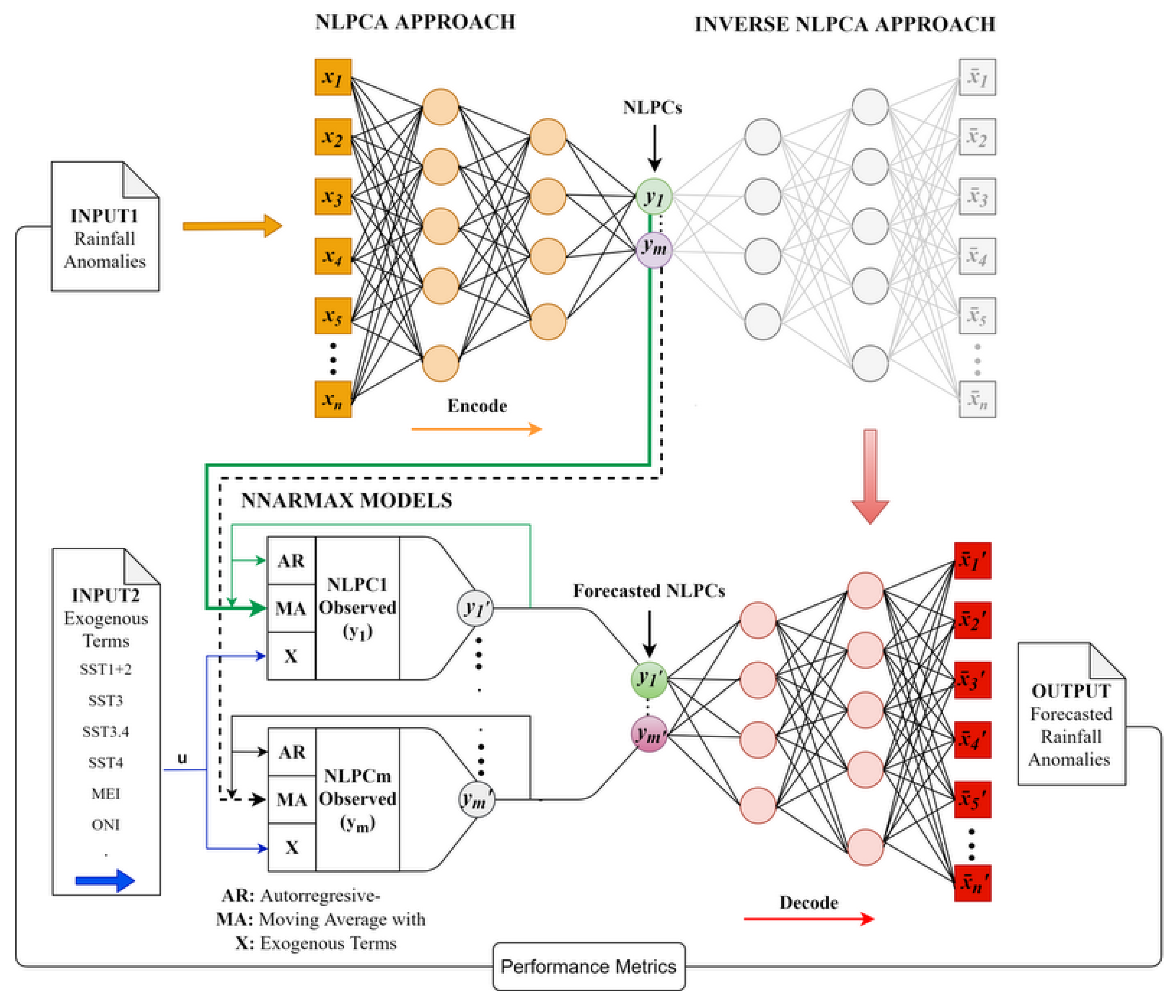
• The Non-linear Principal Component Analysis (NLPCA) allowed the reduction of dimensions of the rainfall anomalies for AR and PR. We get two Non-linear Principal Components (NLPCs) for AR with an explained variance of the original dataset around 73% and one NLPC for PR with an explained variance of around 48%.
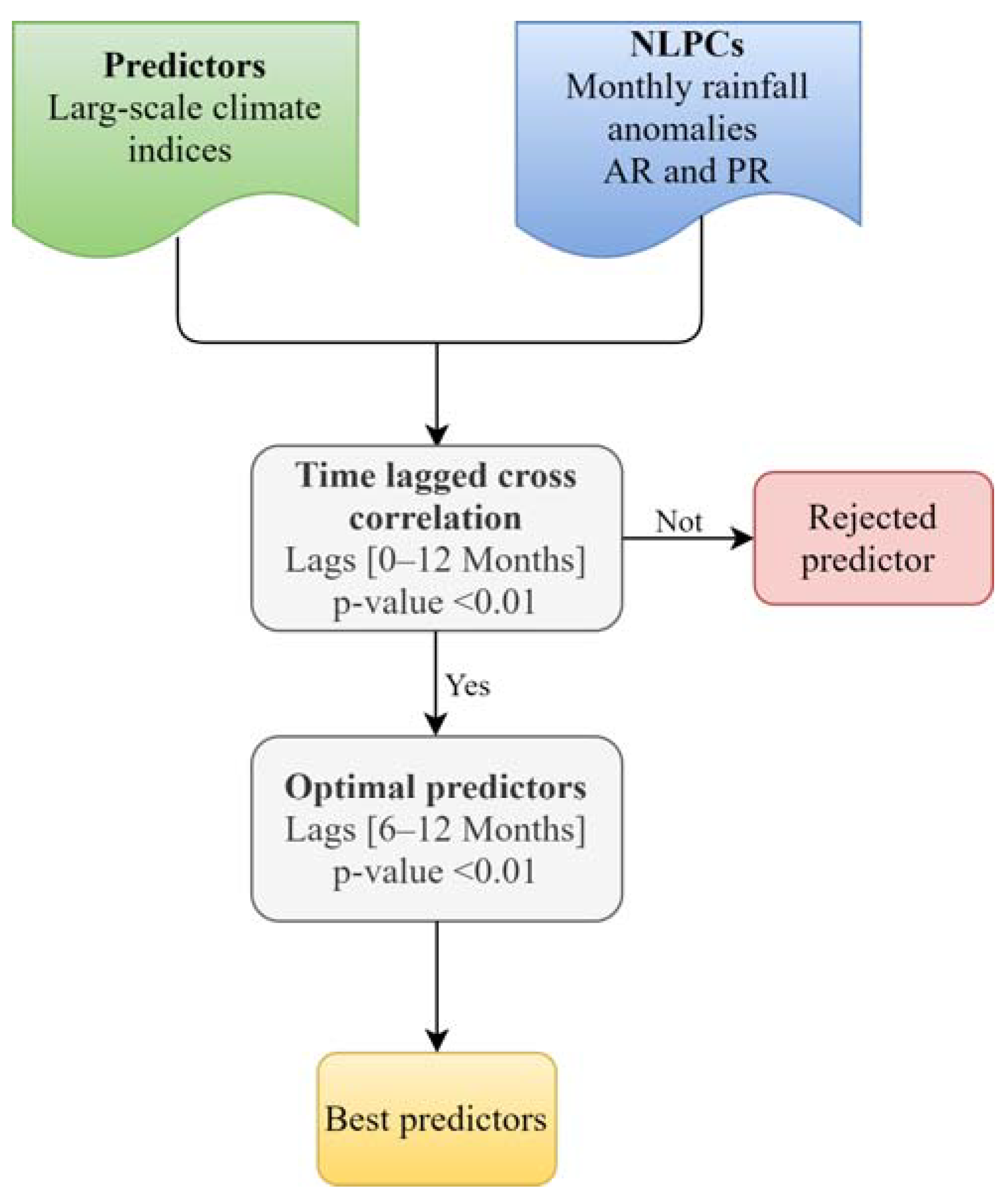
• The analysis of the partial cross-correlations between the main modes of the monthly rainfall variability for AR and PR obtained through NLPCA and the eight large-scale climate indices linked to the ENSO phenomenon helped identify the possible predictors (exogenous variables) for each preliminary NNARMAX model. In this study, the lagged climatic indices from 6 to 12 months with r > 0.128 were considered. The variables selected for the forecasting of NLPC1-AR (NLPC2-AR) were SST1+2, SST3.4, SST4, MEI, ONI, SOI, and PDO (SST1+2, SST3, and MEI), while for NLPC1-PR, they were SST3.4, SST4, MEI, ONI, and SOI.
• The correlation degree measure between NLPCs and climate indices, as well as the relationship persistence, were used for the selection of the best exogenous variables for each Simplified-NNARMAX model. The selected exogenous variables were refined through the backward elimination method. For NLPC1-AR (NLPC2-AR), the selected input variables were SST3.4, MEI, and PDO (SST1+2, SST3, and MEI). For NLPC1-PR, the best predictors were SST3.4 and MEI.
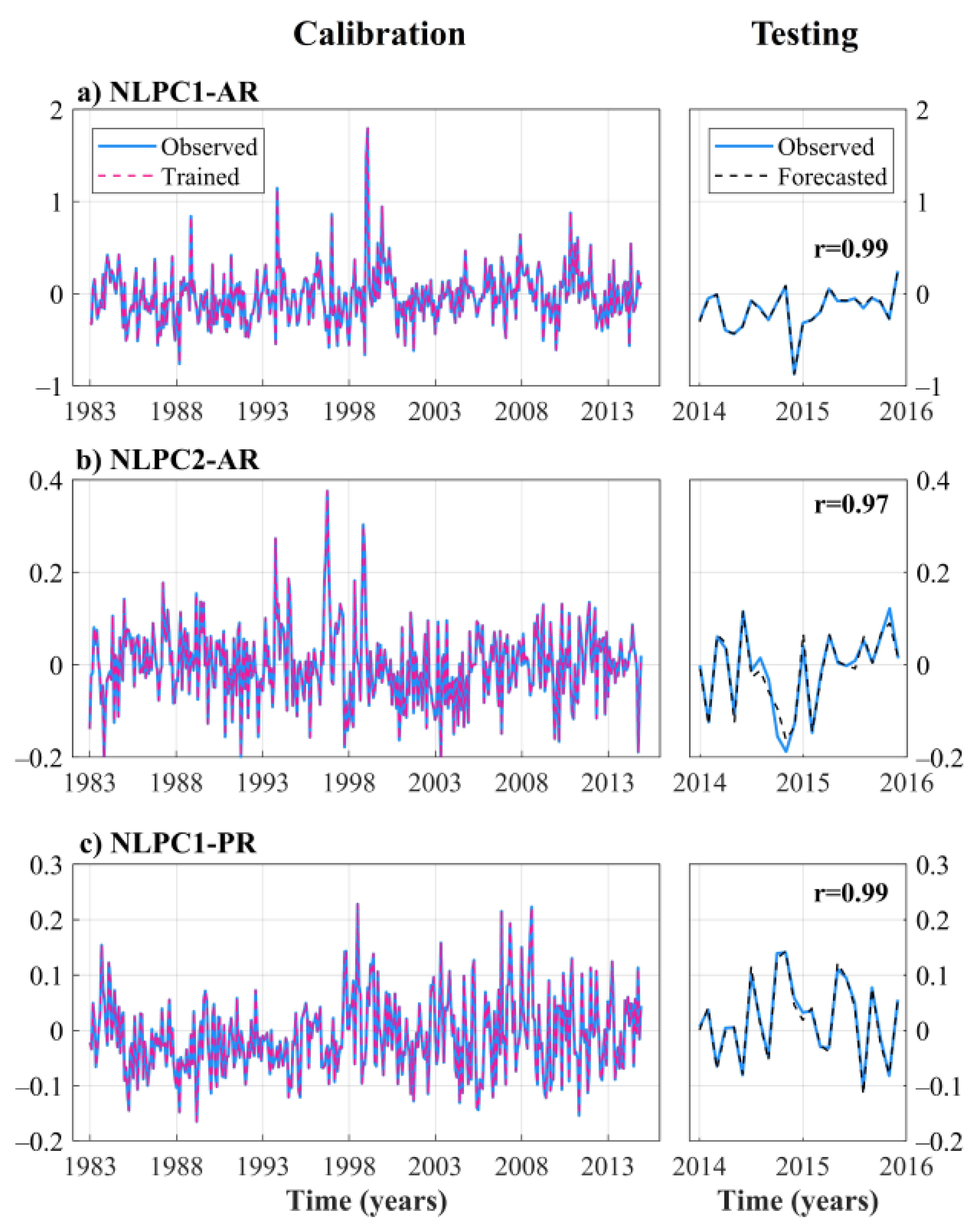
• The performance of the Simplified-NNARMAX model for NLPC1-AR, NLPC2-AR, and NLPC1-PR was measured using Pearson’s correlation between the observed series and the forecasted series. The results showed satisfactory forecasting performance with r values greater than 0.95 for the calibration and testing datasets. Although Simplified-NNARMAX uses less exogenous variables as input than the initial NNARMAX, the performance of each of the models remains preserved, confirming that the selection of exogenous variables was adequate.
• The forecasted NLPCs obtained using Simplified-NNARMAX were used as inputs of the Inverse NLPCA to get the forecasted rainfall anomalies for AR and PR. The results showed suitable forecasting performance both for the AR and for the PR. For AR, the RMSE values were 3.76 and 5.01 mm, while the MAE values were 2.64 and 3.8 mm for the calibration and testing datasets, respectively. While for PR, the RMSE values were 8.5 and 13.99 mm, and MAE values were 6.57 and 10.9 mm for the calibration and testing datasets, respectively. These results indicate that the forecast with ANN approaches is more accurate for AR than for PR. The performance measures of forecasting per each gauge station in both AR and PR support this conclusion. The RMSE values range between 17 and 165 mm, in which the RMSE values in PR are higher than those in AR.
• The ANN approach provided in this study allows the forecasting of the rainfall anomalies of each gauge station that makes up a particular region of interest using as exogenous variables the large-scale climate indices. Furthermore, this model demonstrated the possibility of rainfall forecasting five months in advance for the AR and PR in Southwestern Colombia, providing reasonable forecasting of the months that recorded rainfall above or below the average. This information is relevant for the decision-makers in the Department of Nariño, given that this model provides enough time for the proper planning and management of water resources as well as risk management.

References

- Mehdizadeh, S. Using AR, MA, and ARMA Time Series Models to Improve the Performance of MARS and KNN Approaches in Monthly Precipitation Modeling under Limited Climatic Data. Water Resour. Manag. 2020, 34, 263–282. [Google Scholar] [CrossRef]
- Belayneh, A.; Adamowski, J.; Khalil, B.; Ozga-Zielinski, B. Long-Term SPI Drought Forecasting in the Awash River Basin in Ethiopia Using Wavelet Neural Network and Wavelet Support Vector Regression Models. J. Hydrol. 2014, 508, 418–429. [Google Scholar] [CrossRef]
- Hossain, I.; Rasel, H.; Imteaz, M.A.; Mekanik, F. Long-Term Seasonal Rainfall Forecasting Using Linear and Non-Linear Modelling Approaches: A Case Study for Western Australia. Meteorol. Atmos. Phys. 2020, 132, 131–141. [Google Scholar] [CrossRef]
- Montealegre, B.; Edgar, J.; Caicedo, J.D.P. La Variabilidad Climática Interanual Asociada al ciclo El Niño-La Niña-Oscilación del Sur y su efecto en el patrón pluviométrico de Colombia. Meteorol. Colomb. 2000, 2, 7–21. [Google Scholar]
- Solomon, S.; Qin, D.; Manning, M.; Chen, Z.; Marquis, M.; Averyt, K.B.; Tignor, M.; Miller, H.L. Climate Change 2007: The Physical Science Basis. Contribution of Working Group I to the Fourth Assessment Report of the Intergovernmental Panel on Climate Change; Cambridge University: Cambridge, UK; New York, NY, USA, 2007; Volume 996, pp. 434–497. Available online: https://www.ipcc.ch/site/assets/uploads/2018/05/ar4_wg1_full_report-1.pdf (accessed on 14 July 2020).
- Hastenrath, S.; Greischar, L. Further Work on the Prediction of Northeast Brazil Rainfall Anomalies. J. Clim. 1993, 6, 743–758. [Google Scholar] [CrossRef] [Green Version]
- Zhu, Z.; Li, T. The Statistical Extended-Range (10–30-day) Forecast of Summer Rainfall Anomalies over the Entire China. Clim. Dyn. 2017, 48, 209–224. [Google Scholar] [CrossRef]
- Krishnamurti, T.; Stefanova, L.; Chakraborty, A.; TSV, V.; Cocke, S.; Bachiochi, D.; Mackey, B. Seasonal Forecasts of Precipitation Anomalies for North American and Asian monsoons. J. Meteorol. Soc. Jpn. Ser. II 2002, 80, 1415–1426. [Google Scholar] [CrossRef] [Green Version]
- Kang, J.; Wang, H.; Yuan, F.; Wang, Z.; Huang, J.; Qiu, T. Prediction of Precipitation Based on Recurrent Neural Networks in Jingdezhen, Jiangxi Province, China. Atmosphere 2020, 11, 246. [Google Scholar] [CrossRef] [Green Version]
- Ihara, C.; Kushnir, Y.; Cane, M.A.; De la Pena, V.H. Indian Summer Monsoon Rainfall and Its Link with ENSO and Indian Ocean Climate Indices. Int. J. Clim. J. R. Meteorol. Soc. 2007, 27, 179–187. [Google Scholar] [CrossRef]
- Hossain, I.; Rasel, H.; Imteaz, M.A.; Mekanik, F. Long-Term Seasonal Rainfall Forecasting: Efficiency of Linear Modelling Technique. Environ. Earth Sci. 2018, 77, 280. [Google Scholar] [CrossRef]
- Rahman, M.A.; Yunsheng, L.; Sultana, N. Analysis and Prediction of Rainfall Trends over Bangladesh using Mann–Kendall, Spearman’s rho Tests and ARIMA Model. Meteorol. Atmos. Phys. 2017, 129, 409–424. [Google Scholar] [CrossRef]
- Bang, S.; Bishnoi, R.; Chauhan, A.S.; Dixit, A.K.; Chawla, I. Fuzzy Logic based Crop Yield Prediction using Temperature and Rainfall parameters predicted through ARMA, SARIMA, and ARMAX models. In Proceedings of the 2019 Twelfth International Conference on Contemporary Computing (IC3), Noida, India, 8–10 August 2019; pp. 1–6. [Google Scholar]
- Ebtehaj, I.; Bonakdari, H.; Zeynoddin, M.; Gharabaghi, B.; Azari, A. Evaluation of Preprocessing Techniques for Improving the Accuracy of Stochastic Rainfall Forecast Models. Int. J. Environ. Sci. Technol. 2020, 17, 505–524. [Google Scholar] [CrossRef]
- Khalili, N.; Khodashenas, S.R.; Davary, K.; Baygi, M.M.; Karimaldini, F. Prediction of Rainfall Using Artificial Neural Networks for Synoptic Station of Mashhad: A Case Study. Arab. J. Geosci. 2016, 9, 624. [Google Scholar] [CrossRef]
- Alhamshry, A.; Fenta, A.A.; Yasuda, H.; Shimizu, K.; Kawai, T. Prediction of Summer Rainfall over the Source Region of the Blue Nile by Using Teleconnections Based on Sea Surface Temperatures. Theor. Appl. Clim. 2019, 137, 3077–3087. [Google Scholar] [CrossRef]
- Dikshit, A.; Pradhan, B.; Alamri, A.M. Temporal Hydrological Drought Index Forecasting for New South Wales, Australia Using Machine Learning Approaches. Atmosphere 2020, 11, 585. [Google Scholar] [CrossRef]
- Mishra, A.; Desai, V. Drought Forecasting Using Feed-Forward Recursive Neural Network. Ecol. Model. 2006, 198, 127–138. [Google Scholar] [CrossRef]
- Somvanshi, V.; Pandey, O.; Agrawal, P.; Kalanker, N.; Prakash, M.R.; Chand, R. Modeling and Prediction of Rainfall Using Artificial Neural Network and ARIMA Techniques. J. Ind. Geophys. Union 2006, 10, 141–151. [Google Scholar]
- Chattopadhyay, S.; Chattopadhyay, G. Univariate Modelling of Summer-Monsoon Rainfall Time Series: Comparison between ARIMA and ARNN. Comptes Rendus Geosci. 2010, 342, 100–107. [Google Scholar] [CrossRef]
- Tasadduq, I.; Rehman, S.; Bubshait, K. Application of Neural Networks for the Prediction of Hourly Mean Surface Temperatures in Saudi Arabia. Renew. Energy 2002, 25, 545–554. [Google Scholar] [CrossRef]
- Montazerolghaem, M.; Vervoort, W.; Minasny, B.; McBratney, A. Spatiotemporal Monthly Rainfall Forecasts for South-Eastern and Eastern Australia Using Climatic Indices. Theor. Appl. Climatol. 2016, 124, 1045–1063. [Google Scholar] [CrossRef]
- Poveda, G.; Waylen, P.R.; Pulwarty, R.S. Annual and Inter-Annual Variability of the Present Climate in Northern South America and Southern Mesoamerica. Palaeogeogr. Palaeoclimatol. Palaeoecol. 2006, 234, 3–27. [Google Scholar] [CrossRef]
- Carvajal, Y.; Grisales, C.; Mateus, J. Correlación de variables macroclimáticas del Océano Pacífico con los caudales en los ríos interandinos del Valle del Cauca (Colombia). Rev. Peru. Biol. 1999, 6, 9–17. [Google Scholar] [CrossRef] [Green Version]
- Poveda, G.; Vélez, J.; Mesa, O.; Hoyos, C.; Mejía, J.F.; Barco, O.J.; Correa, P.L. Influencia de fenómenos macroclimáticos sobre el ciclo anual de la hidrología colombiana: Cuantificación lineal, no lineal y Percentiles Probabilísticos. Meteorol. Colomb. 2002, 6, 121–130. [Google Scholar]
- Poveda, G. La hidroclimatología de Colombia: Una síntesis desde la escala inter-decadal hasta la escala diurna. Rev. Acad. Colomb. Cienc. 2004, 28, 201–222. [Google Scholar]
- Puertas Orozco, O.L.; Carvajal Escobar, Y. Incidence of El Niño Southern Oscillation in the Precipitation and the Temperature of the Air in Colombia, Using Climate Explorer. Ing. Desarro. 2008, 23, 104–118. [Google Scholar]
- Tootle, G.A.; Piechota, T.C.; Gutiérrez, F. The Relationships between Pacific and Atlantic Ocean Sea Surface Temperatures and Colombian Streamflow Variability. J. Hydrol. 2008, 349, 268–276. [Google Scholar] [CrossRef]
- Rojo, J.D.; Carvajal, L.F. Predicción no Lineal de caudales Utilizando Variables Macroclimáticas y análisis Espectral Singular. Tecnol. Cienc. Agua 2010, 1, 59–73. [Google Scholar]
- Ávila Díaz, Á.J.; Carvajal Escobar, Y.; Gutiérrez Serna, S.E. Análisis de la influencia de El Niño y La Niña en la oferta hídrica mensual de la cuenca del río Cali. Tecnura 2013, 18, 120–133. [Google Scholar]
- Rodríguez-Rubio, E. A Multivariate Climate Index for the Western Coast of Colombia. Adv. Geosci. 2013, 33, 21–26. [Google Scholar] [CrossRef] [Green Version]
- Restrepo, J.C.; Higgins, A.; Escobar, J.; Ospino, S.; Hoyos, N. Contribution of Low-Frequency Climatic–Oceanic Oscillations to Streamflow Variability in Small, Coastal Rivers of the Sierra Nevada de Santa Marta (Colombia). Hydrol. Earth Syst. Sci. 2019, 23, 2379–2400. [Google Scholar] [CrossRef] [Green Version]
- Cerón, W.; Carvajal-Escobar, Y.; Andreoli, R.V.; Kayano, M.T.; Gonzáles, N. Spatio-Temporal Variability of the Droughts in Cali, Colombia and Their Relationships with the El Niño-Southern Oscillation (ENSO) between 1971 and 2011. Atmósfera 2020, 33, 51–69. [Google Scholar] [CrossRef]
- Canchala, T.; Loaiza Cerón, W.; Francés, F.; Carvajal-Escobar, Y.; Andreoli, R.V.; Kayano, M.T.; Alfonso-Morales, W.; Caicedo-Bravo, E.; Ferreira de Souza, R.A. Streamflow Variability in Colombian Pacific Basins and Their Teleconnections with Climate Indices. Water 2020, 12, 526. [Google Scholar] [CrossRef] [Green Version]
- Canchala, T.; Alfonso-Morales, W.; Loaiza Cerón, W.; Carvajal-Escobar, Y.; Caicedo-Bravo, E. Teleconnections between Monthly Rainfall Variability and Large-Scale Climate Indices in Southwestern Colombia. Water 2020, 12, 1863. [Google Scholar] [CrossRef]
- Enfield, D.B.; Mestas-Nuñez, A.M. Global Modes of ENSO and non-ENSO Sea Surface Temperature Variability and Their Associations with Climate. El Niño South. Oscil. Multiscale Var. Global Reg. Impacts 2000, 89–112. Available online: https://www.aoml.noaa.gov/phod/docs/enfield/final_proofs.pdf (accessed on 30 July 2019).
- Guenni, L.B.; García, M.; Munoz, A.G.; Santos, J.L.; Cedeño, A.; Perugachi, C.; Castillo, J. Predicting Monthly Precipitation along Coastal Ecuador: ENSO and Transfer Function Models. Theor. Appl. Clim. 2017, 129, 1059–1073. [Google Scholar] [CrossRef]
- Jiang, R.; Wang, Y.; Xie, J.; Zhao, Y.; Li, F.; Wang, X. Assessment of Extreme Precipitation Events and Their Teleconnections to El Niño Southern Oscillation, A Case Study in the Wei River Basin of China. Atmos. Res. 2019, 218, 372–384. [Google Scholar] [CrossRef]
- Canchala, T.; Carvajal-Escobar, Y.; Alfonso-Morales, W.; Loaiza, W.; Caicedo, E. Estimation of Missing Data of Monthly Rainfall in Southwestern Colombia using Artificial Neural Networks. Data Brief 2019. [Google Scholar] [CrossRef]
- Scholz, M.; Kaplan, F.; Guy, C.L.; Kopka, J.; Selbig, J. Non-linear PCA: A Missing Data Approach. Bioinformatics 2005, 21, 3887–3895. [Google Scholar] [CrossRef] [Green Version]
- Poveda, G.; Álvarez, D.M.; Rueda, Ó.A. Hydro-Climatic Variability over the Andes of Colombia Associated with ENSO: A Review of Climatic Processes and Their Impact on One of the Earth’s Most Important Biodiversity Hotspots. Clim. Dyn. 2011, 36, 2233–2249. [Google Scholar] [CrossRef]
- Enciso, A.M.; Carvajal-Escobar, Y.; Sandoval, M.C. Hydrological Analysis of Historical Floods in the Upper Valley of Cauca River: Análisis hidrológico de las crecientes históricas del río Cauca en su valle alto. Ing. Y Compet. 2016, 18, 47–58. [Google Scholar]
- Trenberth, K. The Climate Data Guide: Nino SST Indices (Nino 1+ 2, 3, 3.4, 4; ONI and TNI). Available online: https://climatedataguide.ucar.edu/climate-data/nino-sst-indices-nino-12-3-34-4-oni-and-tni (accessed on 18 January 2019).
- L’Heureux, M.L.; Collins, D.C.; Hu, Z.-Z. Linear Trends in Sea Surface Temperature of the Tropical Pacific Ocean and Implications for the El Niño-Southern Oscillation. Clim. Dyn. 2013, 40, 1223–1236. [Google Scholar] [CrossRef] [Green Version]
- Wolter, K.; Timlin, M.S. El Niño/Southern Oscillation Behaviour Since 1871 as Diagnosed in An Extended Multivariate ENSO Index (MEI. ext). Int. J. Clim. 2011, 31, 1074–1087. [Google Scholar] [CrossRef]
- Hsieh, W.W. Nonlinear Principal Component Analysis by Neural Networks. Tellus A: Dyn. Meteorol. Oceanogr. 2001, 53, 599–615. [Google Scholar] [CrossRef] [Green Version]
- Scholz, M. Validation of Nonlinear PCA. Neural Process. Lett. 2012, 36, 21–30. [Google Scholar] [CrossRef]
- Hsieh, W.W.; Tang, B. Applying Neural Network Models to Prediction and Data Analysis in Meteorology and Oceanography. Bull. Am. Meteorol. Soc. 1998, 79, 1855–1870. [Google Scholar] [CrossRef]
- Monahan, A.H. Nonlinear Principal Component Analysis by Neural Networks: Theory and Application to the Lorenz System. J. Clim. 1999, 13, 821–835. [Google Scholar] [CrossRef]
- Monahan, A.H. Nonlinear Principal Component Analysis: Tropical Indo–Pacific Sea Surface Temperature and Sea Level Pressure. J. Clim. 2001, 14, 219–233. [Google Scholar] [CrossRef]
- Miró, J.J.; Caselles, V.; Estrela, M.J. Multiple Imputation of Rainfall Missing Data in the Iberian Mediterranean Context. Atmos. Res. 2017, 197, 313–330. [Google Scholar] [CrossRef]
- Kenfack, C.S.; Mkankam, F.K.; Alory, G.; Du Penhoat, Y.; Hounkonnou, M.N.; Vondou, D.A.; Nfor, G.B. Sea Surface Temperature Patterns in the Tropical Atlantic: Principal Component Analysis and Nonlinear Principal Component Analysis. Terr. Atmos. Ocean. Sci. 2017, 28, 395–410. [Google Scholar] [CrossRef] [Green Version]
- Djibo, A.G.; Karambiri, H.; Seidou, O.; Sittichok, K.; Philippon, N.; Paturel, J.E.; Saley, H.M. Linear and Non-Linear Approaches for Statistical Seasonal Rainfall Forecast in the Sirba Watershed Region (Sahel). Climate 2015, 3, 727–752. [Google Scholar] [CrossRef]
- Lee, J.; Kim, C.-G.; Lee, J.E.; Kim, N.W.; Kim, H. Application of Artificial Neural Networks to Rainfall Forecasting in the Geum River Basin, Korea. Water 2018, 10, 1448. [Google Scholar] [CrossRef] [Green Version]
- Sumi, S.M.; Zaman, M.F.; Hirose, H. A Rainfall Forecasting Method Using Machine Learning Models and Its Application to the Fukuoka City Case. Int. J. Appl. Math. Comput. Sci. 2012, 22, 841–854. [Google Scholar] [CrossRef]
- De Vos, N.; Rientjes, T. Constraints of Artificial Neural Networks for Rainfall-Runoff Modelling: Trade-Offs in Hydrological State Representation and Model Evaluation. Hydrol. Earth Syst. Sci. 2005, 9, 111–126. [Google Scholar] [CrossRef] [Green Version]
- Franch, G.; Nerini, D.; Pendesini, M.; Coviello, L.; Jurman, G.; Furlanello, C. Precipitation Nowcasting with Orographic Enhanced Stacked Generalization: Improving Deep Learning Predictions on Extreme Events. Atmosphere 2020, 11, 267. [Google Scholar] [CrossRef] [Green Version]
- Hall, R.J.; Wei, H.L.; Hanna, E. Complex Systems Modelling for Statistical Forecasting of Winter North Atlantic Atmospheric Variability: A New Approach to North Atlantic Seasonal Forecasting. Q. J. R. Meteorol. Soc. 2019, 145, 2568–2585. [Google Scholar] [CrossRef]
- Kim, T.; Shin, J.-Y.; Kim, H.; Kim, S.; Heo, J.-H. The Use of Large-Scale Climate Indices in Monthly Reservoir Inflow Forecasting and Its Application on Time Series and Artificial Intelligence Models. Water 2019, 11, 374. [Google Scholar] [CrossRef] [Green Version]
- May, R.; Dandy, G.; Maier, H. Review of Input Variable Selection Methods for Artificial Neural Networks. Artif. Neural Netw.-Methodol. Adv. Biomed. Appl. 2011, 10, 16004. [Google Scholar]
- Scholz, M.; Vigário, R. Nonlinear PCA: A new hierarchical approach. In Proceedings of the ESANN, Bruges, Belgium, 24–26 April 2002; pp. 439–444. [Google Scholar]
- Stanski, H.R.; Wilson, L.J.; Burrows, W.R. Survey of Common Verification Methods in Meteorology. WMO. World Weather Watch Technical Report (8). 1989. Available online: https://www.cawcr.gov.au/projects/verification/Stanski_et_al/Stanski_et_al.html (accessed on 27 February 2020).
- Tedeschi, R.G.; Cavalcanti, I.F.; Grimm, A.M. Influences of Two Types of ENSO on South American Precipitation. Int. J. Climatol. 2012, 33, 1382–1400. [Google Scholar] [CrossRef]
- Córdoba-Machado, S.; Palomino-Lemus, R.; Gámiz-Fortis, S.R.; Castro-Díez, Y.; Esteban-Parra, M.J. Influence of Tropical Pacific SST on Seasonal Precipitation in Colombia: Prediction Using El Niño and El Niño Modoki. Clim. Dyn. 2015, 44, 1293–1310. [Google Scholar] [CrossRef]
- Navarro, E.; Vieira, C.; Arias, P. Spatiotemporal Variability of the Precipitation in Colombia during ENSO Events. In Proceedings of the XV Seminario Iberoamericano de Redes de Agua y Drenaje, SEREA2017, Bogotá, Colombia, 27–30 November 2017. [Google Scholar]
- Montealegre, J. Estudio de la Variabilidad Climática de la Precipitación en Colombia Asociada a Procesos Oceánicos y Atmosféricos de Meso y Gran Escala; IDEAM: Bogotá, Colombia, 2009. [Google Scholar]
- Campozano, L.; Célleri, R.; Trachte, K.; Bendix, J.; Samaniego, E. Rainfall and Cloud Dynamics in the Andes: A Southern Ecuador Case Study. Adv. Meteorol. 2016, 2016. [Google Scholar] [CrossRef] [Green Version]
- Morán-Tejeda, E.; Bazo, J.; López-Moreno, J.I.; Aguilar, E.; Azorín-Molina, C.; Sanchez-Lorenzo, A.; Martínez, R.; Nieto, J.J.; Mejía, R.; Martín-Hernández, N. Climate Trends and Variability in Ecuador (1966–2011). Int. J. Climatol. 2016, 36, 3839–3855. [Google Scholar] [CrossRef] [Green Version]
- Garreaud, R.D.; Vuille, M.; Compagnucci, R.; Marengo, J. Present-Day South American Climate. Palaeogeogr. Palaeoclimatol. Palaeoecol. 2009, 281, 180–195. [Google Scholar] [CrossRef]
- Wang, S.; Huang, J.; He, Y.; Guan, Y. Combined Effects of the Pacific Decadal Oscillation and El Nino-Southern Oscillation on Global Land Dry–Wet Changes. Sci. Rep. 2014, 4, srep06651. [Google Scholar] [CrossRef] [PubMed] [Green Version]
- Córdoba-Machado, S.; Palomino-Lemus, R.; Gámiz-Fortis, S.R.; Castro-Díez, Y.; Esteban-Parra, M.J. Assessing the Impact of El Niño Modoki on Seasonal Precipitation in Colombia. Glob. Planet. Chang. 2015, 124, 41–61. [Google Scholar] [CrossRef]
- Cai, W.; Cowan, T. La Niña Modoki impacts Australia Autumn Rainfall Variability. Geophys. Res. Lett. 2009, 36. [Google Scholar] [CrossRef]
- Ashok, K.; Behera, S.K.; Rao, S.A.; Weng, H.; Yamagata, T. El Niño Modoki and its Possible Teleconnection. J. Geophys. Res. Ocean. 2007, 112. [Google Scholar] [CrossRef]
- Gutiérrez, F.; Dracup, J. An Analysis of the Feasibility of Long-Range Streamflow Forecasting for Colombia Using El Nino–Southern Oscillation Indicators. J. Hydrol. 2001, 246, 181–196. [Google Scholar] [CrossRef]
- Vicente-Serrano, S.M.; Aguilar, E.; Martínez, R.; Martín-Hernández, N.; Azorin-Molina, C.; Sánchez-Lorenzo, A.; El Kenawy, A.; Tomás-Burguera, M.; Moran-Tejeda, E.; López-Moreno, J.I. The Complex Influence of ENSO on Droughts in Ecuador. Clim. Dyn. 2017, 48, 405–427. [Google Scholar] [CrossRef] [Green Version]
- Loaiza Cerón, W.; Andreoli, R.V.; Kayano, M.T.; Ferreira de Souza, R.A.; Canchala, T.; Carvajal, Y. Comparison of Spatial Interpolation Methods for Annual and Seasonal Rainfall in Two Hotspots of Biodiversity in South America. An. Acad. Bras. Cienc. 2020, in press. [Google Scholar]