Optimal Parameter Estimation in Activated Sludge Process Based Wastewater Treatment Practice


1
College of Electrical and Information Engineering, Lanzhou University of Technology, Lanzhou 730050, China
2
School of Engineering, Royal Melbourne Institute of Technology (RMIT University), Melbourne 3000, Australia
3
Key Laboratory of Gansu Advanced Control for Industrial Processes, Lanzhou University of Technology, Lanzhou 730050, China
4
National Demonstration Center for Experimental Electrical and Control Engineering Education, Lanzhou University of Technology, Lanzhou 730050, China
*
Author to whom correspondence should be addressed.
Water 2020, 12(9), 2604; https://doi.org/10.3390/w12092604
Submission received: 3 July 2020
/
Revised: 8 September 2020
/
Accepted: 12 September 2020
/
Published: 17 September 2020
(This article belongs to the Special Issue Mathematical Modeling and Simulations of Wastewater Treatment Processes)
Abstract
:Activated sludge models (ASMs) are often used in the simulation of the wastewater treatment process to evaluate whether the effluent quality parameters of a wastewater treatment plant meet the standards. The premise of successful simulation is to choose appropriate dynamic parameters for the model. A niche based adaptive invasive weed optimization (NAIWO) algorithm is proposed in this paper to find the appropriate kinetic parameters of activated sludge model 1 (ASM1). The niche idea is used to improve the possibility of convergence to the global optimal solution. In addition, the adaptive mechanism and periodic operator are introduced to improve the convergence speed and accuracy of the algorithm. Finally, NAIWO is used to optimize the parameters of ASM1. Comparison with other intelligent algorithms such as invasive weed optimization (IWO), genetic algorithm (GA), and bat algorithm (BA) showed the higher convergence accuracy and faster convergence speed of NAIWO. The results showed that the ASM1 model results agreed with measured data with smaller errors.
1. Introduction
Activated sludge process is a complex biochemical reaction process, which mainly uses the metabolism of microorganisms present in the activated sludge to remove the organic pollutants that are present in the wastewater. Therefore, it will be affected by external conditions such as the environment and the temperature of the wastewater. Activated sludge process is one of the most commonly used wastewater treatment methods, especially for large-scale urban wastewater treatment plants. Activated sludge model 1 (ASM1) was proposed by the International Water Association (IWA) in 1987. The ASM1 is a complex mathematical model with 65 differential equations and 19 kinetic or stoichiometric parameters [1]. ASM1 is the most commonly used and most researched simulation model in the field of activated sludge process [2,3,4,5]. However, in actual wastewater treatment plant applications, due to changes in operating conditions and differences in the external environments, the dynamics or stoichiometric parameters of ASM1 will have to be determined. If the reference parameters provided by IWA are used, they will cause a serious deviation between the model output and the actual results. Therefore, correcting the parameter values of ASM1 for practical applications is the key to the success of the application of the model [6].
In the early days, the methods of parameter identification of environmental models in environmental engineering mainly included trial and error techniques [7], optimization methods based on gradient descent [8], and statistical methods based on random sampling [9,10,11]. However, these methods are inadequate in improving parameter accuracy or convergence speed and it is difficult to obtain satisfactory results with minimum time and effort. Gradient-based optimization methods rely too much on the selection of initial values and tend to converge to a local optimum. The search mechanism of statistical methods is random. When the number of parameters increases, the number of calculation steps will increase exponentially, becoming inefficient in solving complex problems. With the extensive application of genetic algorithms (GA) in various fields [12], meta-heuristic search algorithms are gradually introduced into parameter estimation of the activated sludge process models. Compared with the above methods, a meta-heuristic search algorithm can converge to the global optimal solution with higher probability at a faster speed [13,14]. Kim et al. [15] used GA to estimate the sensitive parameters in ASM1. The results showed that using the optimized parameters to run ASM1 can reduce the error between the predicted and the actual values, and confirms the applicability of a meta-heuristic optimization algorithm in parameter optimization of a nonlinear system model. Du et al. [16] introduced the adaptive step control algorithm to improve the cuckoo search (CS), targeting the shortcomings of the optimization mechanism of the CS algorithm and the slow convergence speed in the later stages. Outcomes show that the improved CS is more effective in the parameter estimation of ASM1.
Invasive weed optimization (IWO) algorithm, proposed by Mehrabian et al. [17] in 2006, is a new type of meta-heuristic optimization algorithm. IWO mimics the strong colonial dominance power of wild grasses by imitating the growth, reproduction, diffusion, and competition of field weeds. It has been widely used in engineering optimization [18,19], fault diagnosis [20], and hybrid algorithm optimization [21]. In the IWO algorithm, as the number of iterations increases, the spatial distribution of the next generation of seeds will gradually narrow, which can ensure that the algorithm has a strong global search ability in the early stages and a strong local search ability in the later stages. However, it also leads to the lack of local search ability in the early stages and the lack of population diversity in the later stages. In order to get better optimization results, it is necessary to improve and fuse the IWO algorithm. Cuevas et al. [21] proposed a hybrid evolutionary method, which combines the search ability of IWO and probability model of an estimated distribution algorithm, making a hybrid method with higher accuracy, efficiency, and robustness. Liu et al. [19] introduced simplified quadratic approximation into the IWO algorithm and the application in the directional pattern synthesis of array antennas showed the effectiveness of the improved IWO algorithm.
In response to the above problems, the niche idea and adaptive mechanism are introduced into the IWO algorithm in this paper and a niche-based adaptive invasive weed optimization (NAIWO) algorithm is proposed. Niche is used to increase the population diversity of the algorithm. Then, a periodic operator and adaptive algorithm are introduced into the adaptive mechanism, so that the standard deviation of the spatial diffusion of individual weeds not only changes with the number of iterations, but also can dynamically change according to the parameters of the periodic operator and the fitness value of the individual. Finally, verified through parameter optimization of ASM1, the effectiveness of the NAIWO algorithm in global convergence ability and convergence speed is proven.
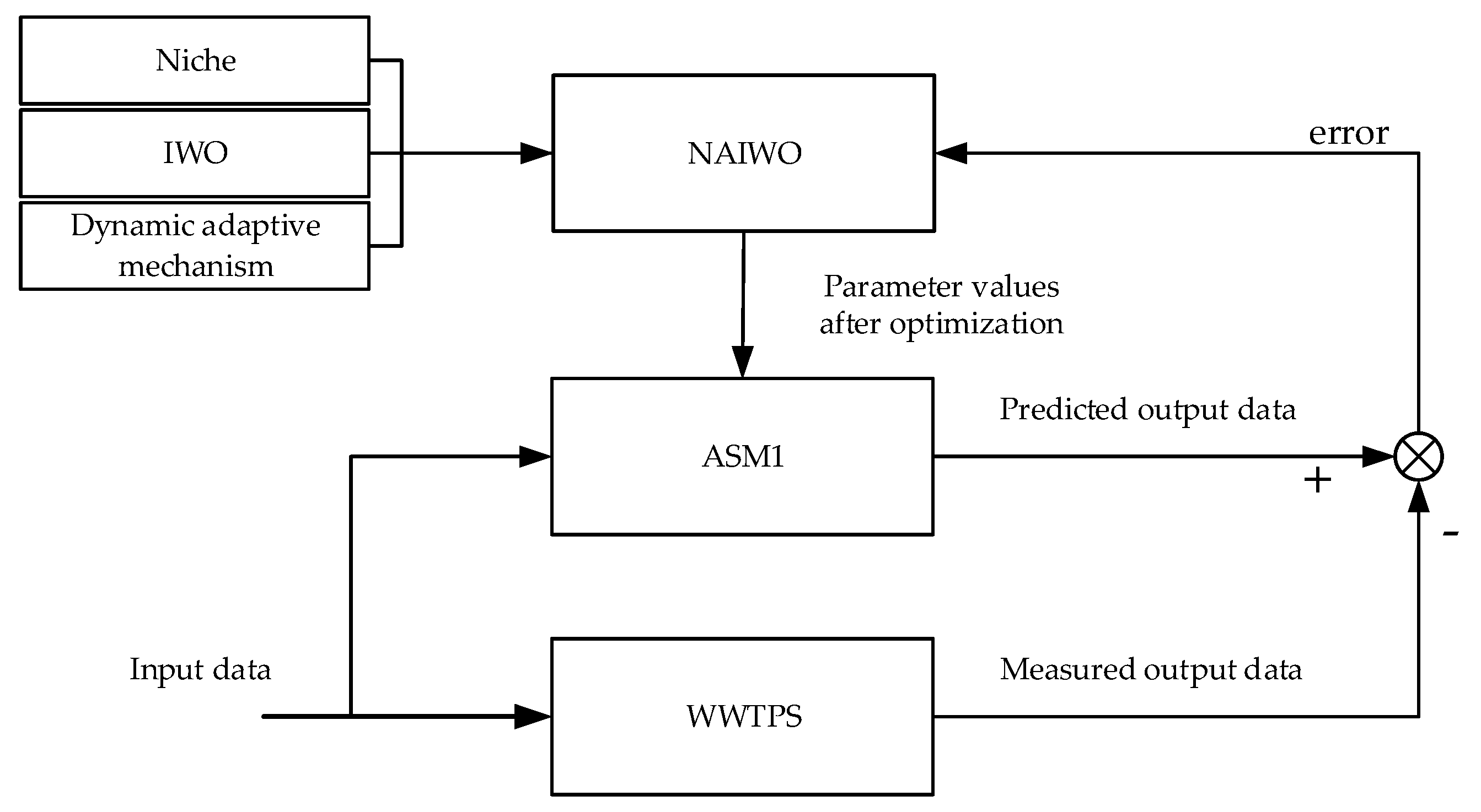
Figure 1 shows the schematic diagram of the process of ASM1 parameter estimation using the NAIWO algorithm. The input data of the wastewater treatment plant is taken as the input data of ASM1. The predicted data of effluent is obtained from the ASM1 model and the error is calculated by comparing the measured and the predicted data. Then, the error is sent to the NAIWO algorithm for parameter optimization. Parameter optimization is repeated until the error is minimized to a desired level.
2. Materials and Methods
2.1. Invasive Weeds Optimization (IWO)
The IWO algorithm imitates the basic process of weed diffusion, growth, propagation, and competitive survival in the field. “Weeds” represent a feasible solution to the problem and “populations” represent the set of all weeds.
The basic steps of IWO can be expressed as follows:
- (1)
- Population initialization. P0 of weeds (feasible solutions) were randomly generated in the solution space (D-dimension). Generally, the size of P0 can be adjusted according to the actual situation.
- (2)
- (Growth and reproduction. After seeds grow and bloom, they produce a new generation of seeds according to their own fitness. The number of seeds produced by the parents is related to the fitness of the parents. The specific relationship is shown in Equation (1):where FN and SN represent the fitness value of the Nth parent and the number of seeds it should produce, respectively; Fmax and Fmin represent the maximum and minimum fitness of the parents, respectively. Smax and Smin represent the maximum and minimum number of seeds produced by individual weeds, respectively. The number of seeds generated is a rounded down number of SN.
- (3)
- Space diffusion. The generated seeds are normally distributed in the D-dimensional space near their parents. The mean value of the normal distribution is 0 and the standard deviation is σiter. The variation of the standard deviation with the number of iterations is shown in Equation (2):where iter and itermax represent the current number of iterations and the maximum number of iterations; σinitial represents the initial standard deviation value; σfinal represents the final standard deviation value; and n represents the nonlinear harmonic coefficient. It is generally ensured that σinitial is greater than σfinal.
- (4)
- Competition exclusion. After several generations of reproduction, environmental resources will not be able to bear the number of offspring produced. The maximum population size is determined as the preset maximum population number Pmax. When Pmax is reached, firstly reproduce freely according to the previous steps. Then, based on the population upper limit requirement, the parents and children are eliminated together according to the adaptive value.
- (5)
- Repeat steps 2 to 4 until the maximum number of iterations is reached or the solution satisfying the required conditions is found.
2.2. Niche-Based Adaptive Invasive Weed Optimization (NAIWO)
It can be seen from Equations (1) and (2) that in the IWO algorithm, the individual weeds of each generation determine the number of next generations according to the degree of fitness, so as to ensure that the excellent individual genes are inherited to the next generation. As the iteration goes on, the diffusion range (i.e., the size of the standard deviation σiter) of the next generation seed is gradually reduced, which ensures that the algorithm has a strong global search ability in the early stages and local search ability in the later stages. However, this also leads to insufficient local search capability in the early stages of the algorithm and later searches only near seeds with higher fitness, resulting in a lack of diversity in the later stages of the algorithm. In order to solve these problems, a niche-based adaptive invasive weed optimization (NAIWO) algorithm is proposed by introducing the idea of a niche and adaptive mechanism.
2.2.1. Dynamic Adaptive Mechanism
In step 3 of the IWO algorithm, the distribution of the next-generation seeds generated by each parent follows the same normal distribution and the standard deviation of its search walking is σiter, which decreases with the number of iterations. Although the global search ability in the early stages and the local search ability in the later stages are considered in this distribution method, the population diversity in the later stage of the algorithm is insufficient, which makes the algorithm fall easily into a local optimum. In this paper, the dynamic adaptive mechanism is introduced into the spatial diffusion step of the IWO algorithm to balance the global and local optimization ability of the algorithm.
The spatial diffusion criterion is shown in Equations (3)–(5):
In the dynamic adaptive spatial diffusion mechanism, the spatial distribution σj of the children generated by each parent is shown in Equations (4) and (5). In Equation (4), a cosine periodic function is employed, where T is a periodic parameter and K is a scaling factor. By adjusting the values of K and T, the dynamic diffusion standard deviation σiter can be changed with a period T between [1/K, K]. For the jth parent‘s weed, the distribution of its offspring σj is also related to its fitness in the population, as shown in Equation (5).
In each iteration, Fmax and Fmin are the maximum and minimum fitness values in the parent population; Fj is the fitness value of the jth parent. The distribution of each generation’s population is not only related to the iteration number (iter), but also has a functional relationship with the fitness of the parent in the population. In the iterative process, the higher the adaptability of the weeds, the larger the number of the next generation seeds and the more centralized the distribution of the next generation, making the seeds continuously concentrate to high adaptability. However, for the parents with low adaptability, the number of seeds produced is less in a larger distribution range, so as to improve the possibility of finding the global optimal solution.
2.2.2. Niche Idea
The niche idea is derived from biology and refers to a living environment under a specific condition. In the evolution process of organisms, they generally always live with the same species and jointly reproduce offspring. Each generation is divided into several classes according to the fitness value and each class can represent a niche. The combination of a niche idea and intelligent algorithm shows strong utility [22,23]. In this paper, the niche idea is introduced into the competitive exclusion step of the IWO algorithm, and the characteristics of classification competition of niche is used to increase the diversity of the population and improve the overall optimization ability of the algorithm.
The determination of the radius R of the niche is based on Equation (6):
where represents the Euclidean distance from the ith weed to the most adaptable weed in the iter iteration; a, b, and k are adjustable parameters. By adjusting their values, we can adjust the rate of change and the start and end values of the radius R of the niche accordingly.
The process of dividing niches is described as follows:
- (1)
- Arrange the weed individuals in the population in descending order according to the degree of fitness. If the population number is greater than the maximum population number Pmax, take the first Pmax weed individuals as the parents for the next generation.
- (2)
- The center (H1) of the first niche is the position of the weed with the highest adaptability, and R is its radius. If the Euclidean distance (d1,i) of the other weeds in the population from the center of niche H1 is less than R, they would be included into the niche H1. Otherwise, it would be excluded.
- (3)
- The second niche, H2, is marked by the weed with the highest adaptability among the rest of the individuals not belonging to H1. Repeat the process (2) until all weeds in the population are tagged.
The steps of NAIWO can be described as follows:
- (1)
- Population and parameter initialization.
- (2)
- Calculate the fitness of each individual weed and arrange all the individual weeds according to the above-mentioned niche classification method.
- (3)
- According to Equation (1), the growth and propagation of weeds are carried out to produce seeds.
- (4)
- According to Equations (3)–(5), the adaptive spatial diffusion based on fitness is carried out.
- (5)
- Solution is considered optimal when the solution meets the requirements or the maximum number is reached.
- (6)
- If the current number of individual weeds Piter is greater than the maximum population number Pmax, go to the competition exclusion process in step 7; otherwise, return back to step 2.
- (7)
- Competition exclusion: Select a certain number of weed individuals from each niche for the next iteration as parents. The number of individuals selected in each niche is related to the ratio of the number of individuals in the niche to the total number of individuals in the population as shown in Equation (7):where Pmax is the maximum population; X(i) represents the number of individuals in the ith niche and sum(X) is the total number of individuals in all niches.
- (8)
- Repeat steps 2 to 7 until the optimal solution is found or the maximum number of iterations is reached.
Based on the above improvement ideas, a new algorithm (NAIWO) with excellent performance is established. To verify the effectiveness of the NAIWO algorithm, we have done a series of optimization performance tests. The results and more information could be found in Appendix A.
2.3. Application: ASM1 Parameter Optimization for Actual Wastewater Treatment Plants
During the operation of a biological wastewater treatment plant, its internal biochemical reaction mechanisms are extremely complex. Therefore, before the ASM1 was proposed, establishing the process model for biological wastewater treatment plants was always difficult and lacked accuracy; this led to difficulties in controlling the effluent water quality to meet increasingly strict standards using controllers.
The purpose of ASM1 is to describe the reaction mechanisms of the activated sludge process as accurately as possible. After selecting the appropriate reaction parameters for ASM1, the reaction processes of an activated sludge plant can be described more accurately, laying the foundation for a precise control of the effluent water quality parameters.
However, for different wastewater treatment plants located in different places, the environmental conditions and inflow conditions may be quite different. If the recommended parameters given by IWA are continued to be used, the model will lack accuracy when predicting the quality of the treated effluent.
2.3.1. Plants and Data Description
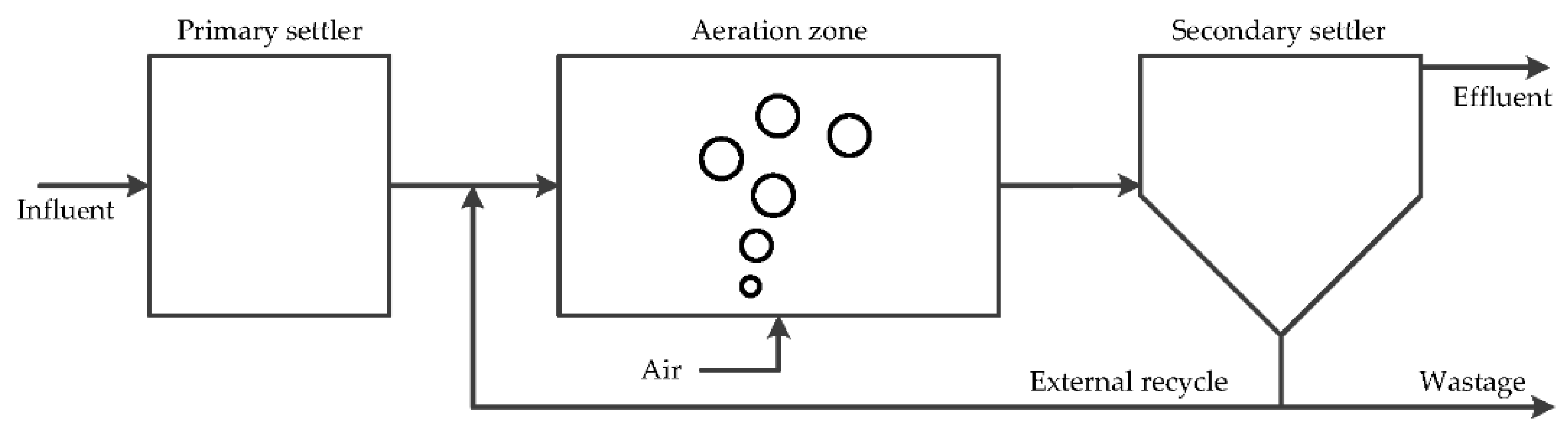
In order to obtain an accurate model of the wastewater treatment plant, the proposed NAIWO algorithm was used to estimate seven important parameters of ASM1, and the process models of two wastewater treatment plants, the Pingliang City Wastewater Treatment Plant (PC-WWTP) in Gansu Province, China and the Wushan County Wastewater Treatment Plant (WC-WWTP) in Tianshui City, Gansu Province, China were established. PC-WWTP is a large full-scale activated sludge process-based wastewater treatment plant with a designed wastewater treatment capacity of 50,000 m3/day and an average daily wastewater inflow of 20,291 m3/day. WC-WWTP is a small biological wastewater treatment plant with a designed wastewater treatment capacity of 8000 m3/day and an average daily wastewater inflow of 5742 m3/day. Figure 2 shows the basic processing of both plants, PC-WWTP and WC-WWTP, based on activated sludge process (ASP).
All the experimental data used in this work comes from the dry weather dynamic inflow and effluent water quality measurement data of these two wastewater treatment plants. The inflow data is collected as an “Influent” input, shown in Figure 2, and the effluent data is collected as an ‘Effluent’ output. The data used in the experiment were measured by the sensors in the two wastewater treatment plants. The inflow wastewater data includes the components of SI, SS, XI, XS, XB,H, XB,A, XP, SO, SNO, SNH, SND, XND, SALK, TSS, and Q0, where TSS represents total amount of solids (mg SS /L) and Q0 stands for influent flow rate (m3/day). The effluent concentration of four representative components, SNH, SNO, SS, and XS, was selected as the standard to judge the accuracy of parameter estimation. A detailed description of these components and reactions is given in Table A5. See more information in Appendix B.
The simulation data were collected in dry weather and the duration was 1 day. The sampling frequency was 15 min, so there were 97 sets of sampling data for computations.
2.3.2. ASM1 Parameter Estimation
The purpose of parameter estimation for ASM1 is to select a set of appropriate parameter values to minimize the errors between the model output and the observed values in the wastewater treatment plant. There are five stoichiometric parameters of biochemical reactions and 14 kinetic parameters involved in ASM1. The correctness of these 19 parameters ensures the accuracy of the ASM1 model in simulating the performance of actual wastewater treatment plants and the specific information of those 19 parameters is shown in Table 1.
Estimation of all the 19 parameters in ASM1 is very complicated. Therefore, seven parameters [24] that have a greater influence on the output results were selected in this section as the estimation objects and the remaining 12 insensitive parameters were used as recommended by the ASM1 model description.
In the process of parameter estimation of ASM1, the sum of squares of relative errors were used as the objective function as shown in Equation (8) in order to minimize the difference between model outputs and observed data:
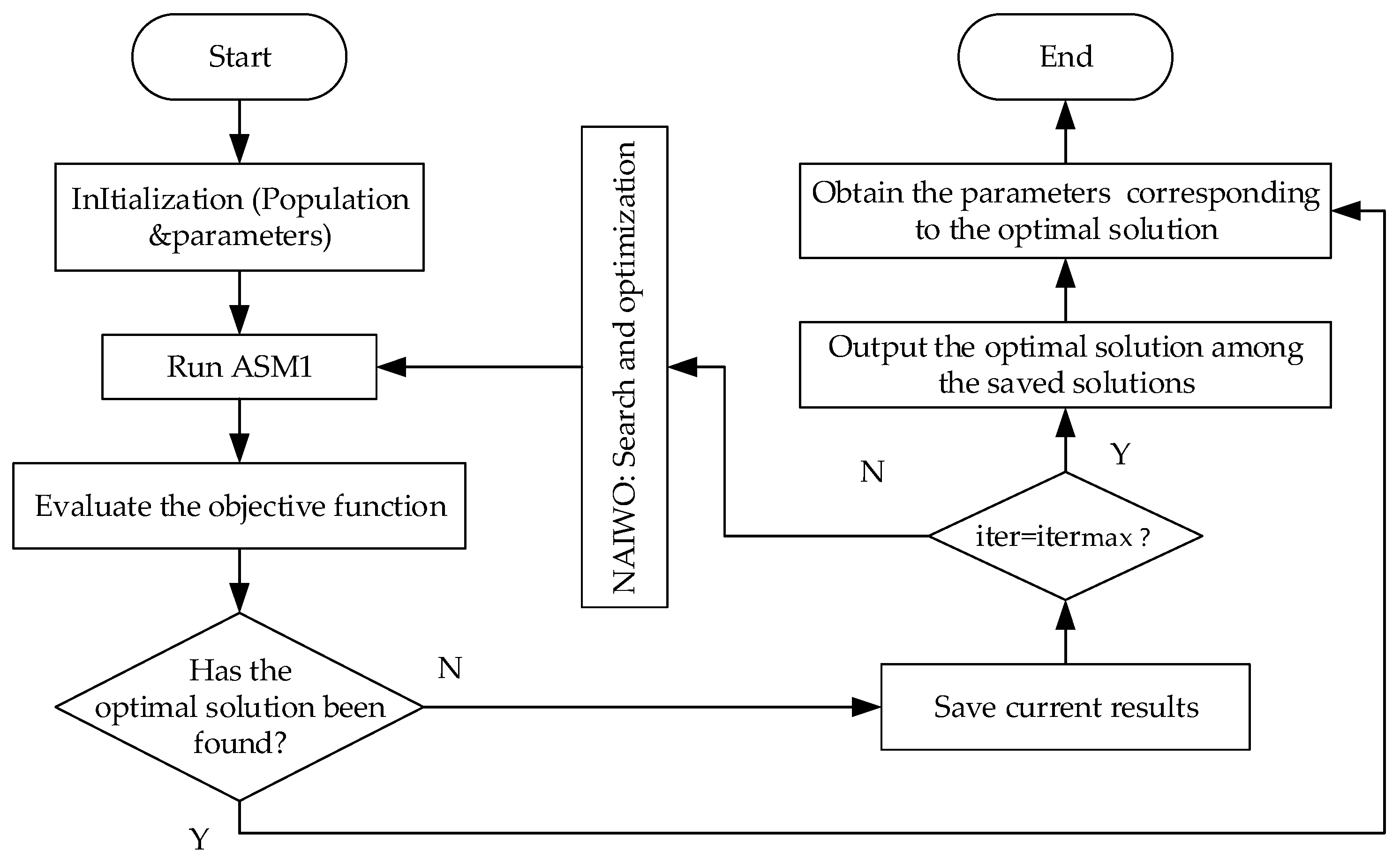
where p is the total number of times the samples were taken and q is the number of effluent quality parameters considered; is the model prediction of the jth effluent quality parameter of the ith sampling time and is the measured value of the jth effluent quality parameter of the ith sampling time. The process of parameter optimization is to find the minimum value of the objective function. Figure 3 shows the flow chart of the NAIWO algorithm used in parameter estimation of the ASM1 model.
By bringing the optimal parameter values estimated by the proposed NAIWO algorithm to run ASM1, this will simulate the effluent quality from an activated sludge plant accurately. In this study, the effluent concentration of ammonia nitrogen (SNH), nitrate nitrogen (SNO), soluble rapidly biodegradable organic matter (SS), and insoluble slowly degradable organic matter (XS) were selected as the objects to verify the validity of the ASM1 parameter estimation.
3. Results and Discussion
In order to prove the advantages of the proposed NAIWO algorithm, seven parameters of ASM1 are estimated by IWO, GA, BA, and NAIWO, respectively. The optimization results are shown in Table 2 (PC-WWTP) and Table 3 (WC-WWTP).
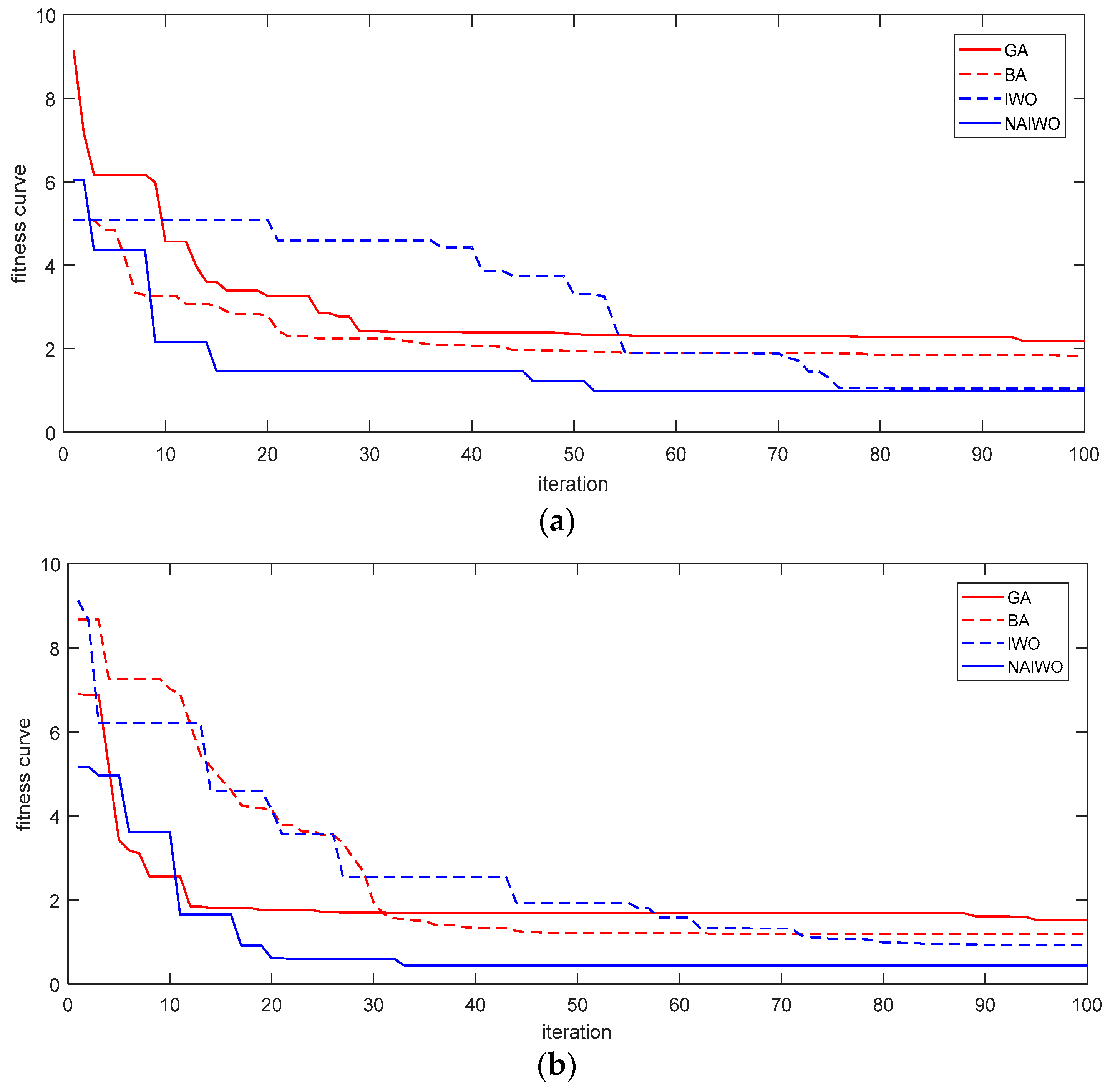
The fitness curves of the four algorithms in the parameter estimation process of ASM1 for the two wastewater treatment plants are shown in Figure 4a,b, respectively. The calculation result of Equation (8) (i.e., the sum of squares of relative errors) is used as the fitness value. Therefore, the fitness value reflects the error between the predicted values by ASM1 and the actual measured values at the wastewater treatment plant. The smaller the error value is, the better the simulation performance.
The shape of fitness curve reflects the change in error during the process of parameter optimization carried out by an algorithm. The faster the fitness curve drops, the faster the convergence speed of the algorithm and the smaller the final fitness value, the higher the convergence accuracy of the algorithm.
It can be seen from the fitness curve shown in Figure 4a (PC-WWTP) that the convergence accuracies of GA and BA are significantly lower than that of IWO and NAIWO. For IWO, its convergence accuracy is only slightly less than NAIWO, but the convergence speed (declining speed of the curve) is significantly lower than NAIWO. In addition, in the process of estimating the parameters of WC-WWTP, the final fitness value of NAIWO is significantly smaller than the other three algorithms and the falling speed of the fitness curve is also significantly higher than that of the other three.
In summary, the NAIWO algorithm can achieve the minimum error with the fastest speed in comparison with GA, BA, and IWO, whether it is applied for large (PC-WWTP) or small (WC-WWTP) wastewater treatment plants.
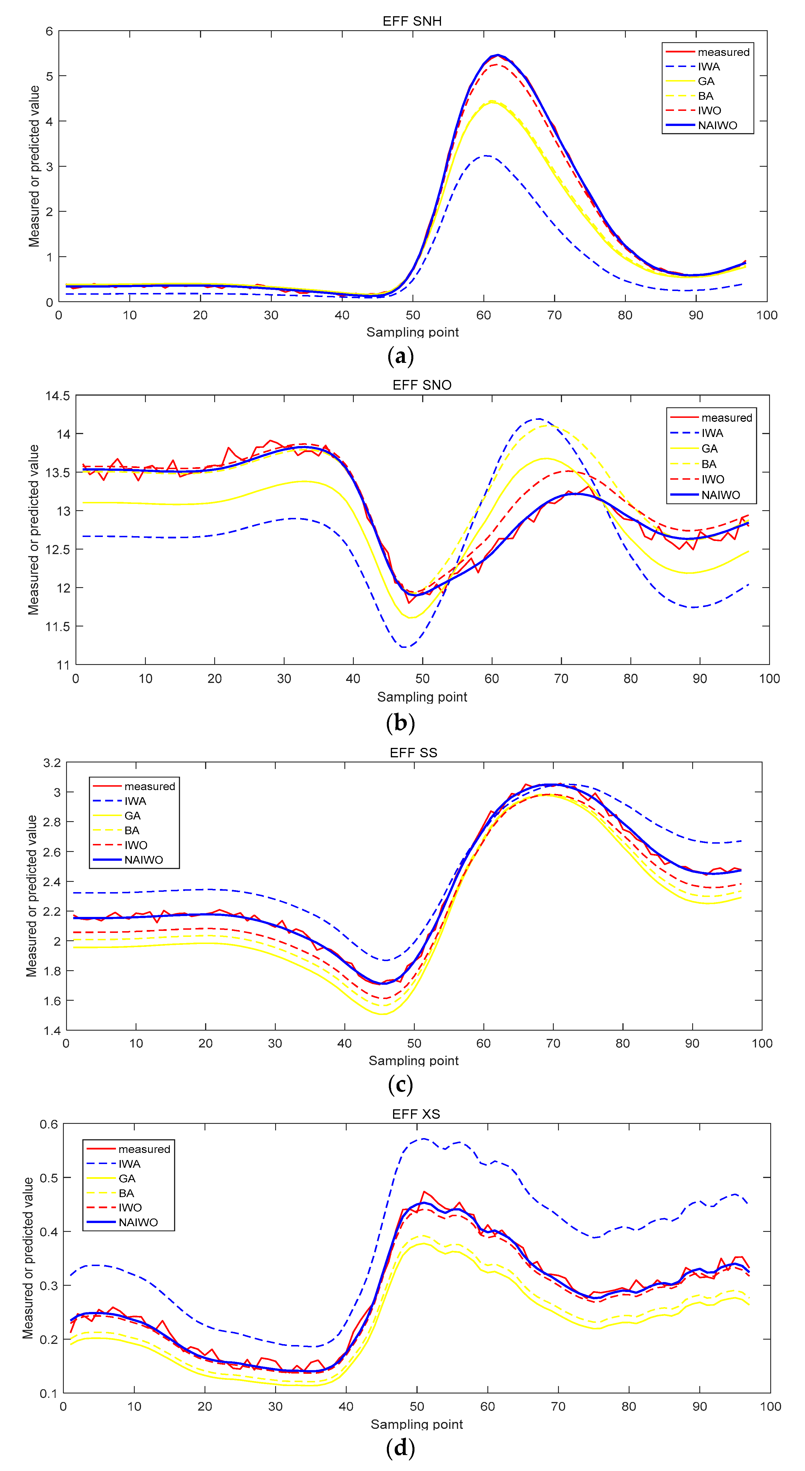
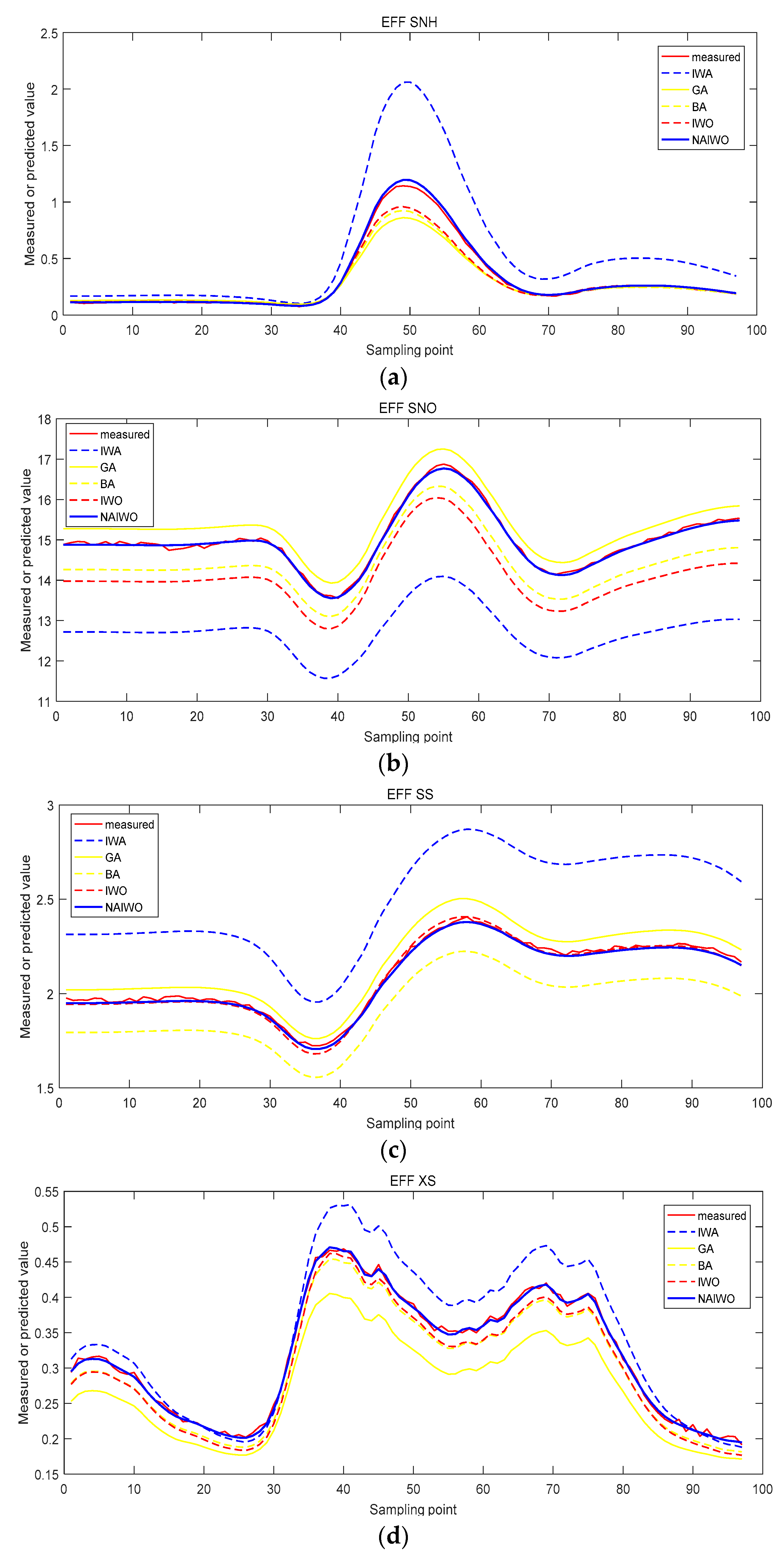
In order to further verify the effect of parameter estimation, the parameters estimated by the four algorithms were introduced into ASM1 and the error between the predicted data of the ASM1 and the actual effluent data were compared. Ammonia nitrogen (SNH), nitrate nitrogen (SNO), soluble rapidly biodegradable organic matter (SS), and insoluble slowly degradable organic matter (XS) were used as comparative objects. The comparison curves of predicted values and actual values are shown in Figure 5 and Figure 6.
Figure 5a–d and Figure 6a–d are the effluent SNH, SNO, SS, and XS concentration curves of PC-WWTP and WC-WWTP. The red solid line in the figure represents the actual measured water quality parameters of the two wastewater treatment plants. The closer the other curves are to the red solid line, the smaller the error during the simulation of ASM1 and the higher the accuracy of the parameter estimation.
It can be seen that when the recommended parameter values given by IWA were used, the prediction errors of the model were larger. After optimal parameters were obtained by GA, BA, IWO, and NAIWO algorithms, the prediction accuracy was improved to a certain extent.
In Figure 5a, when the concentration of effluent SNH was small, the prediction errors of the four algorithms were small. When the concentration increased rapidly (the 50th–70th sampling points), the four algorithms had obvious differences. Only the parameters estimated by NAIWO could track the change of SNH concentration well. Meanwhile, it can be seen from Figure 5b–d that the NAIWO algorithm had the best performance with the highest tracking accuracy to the measured data of SNO, SS, and XS.
As can be seen from Figure 6, IWO had a similar prediction accuracy to that of NAIWO only when predicting the SS concentration of the effluent. The prediction errors of the NAIWO algorithm for the effluent concentration of SNH, SNO, and XS were much smaller than the GA, BA, and IWO algorithms.
According to the results simulated by ASM1 for the effluent quality of two wastewater treatment plants, it was found that the parameters estimated by GA, BA, and IWO can reduce the prediction error of ASM1 to a certain extent, while the parameters estimated by NAIWO can produce the minimum prediction error. Therefore, NAIWO is more effective in optimizing ASM1 parameters than GA, BA, and IWO.
The results illustrate that for both the Pingliang City Wastewater Treatment Plant (PC-WWTP) and Wushan County Wastewater Treatment Plant (WC-WWTP), the proposed NAIWO algorithm is effective for the optimization of the seven sensitive parameters of ASM1. The ASM1 model with optimized parameters can effectively predict the effluent quality of Pingliang City Wastewater Treatment Plant and Wushan County Wastewater Treatment Plant. These two wastewater treatment plants represent different scales with respect to treatment capacity and different water quality environments. The successful application of NAIWO in ASM1 parameter estimation for these two wastewater treatment plants gives confidence for NAIWO to be applied to other activated sludge process based wastewater treatment plants.
4. Conclusions
In this paper, a niche-based adaptive invasion weed optimization (NAIWO) algorithm was proposed to overcome the shortcomings of invasive weed optimization (IWO), such as insufficient local search ability in the early stages of the iteration and insufficient population diversity in the later stages. On the basis of high convergence accuracy, the NAIWO algorithm achieved the balance of global convergence ability and convergence speed and the stability of the algorithm was also improved.
IWA recommended model parameters cannot be used to run ASM1 for each and every activated sludge process based wastewater treatment plants as they are being operated under different environmental conditions. Thus, seven sensitive parameters of the ASM1 model were estimated by the NAIWO algorithm using the data obtained from a large and a small to medium scale treatment plant. In tracking the effluent parameters of those two actual wastewater treatment plants, the NAIWO algorithm achieved better prediction accuracy than the GA, BA, and IWO algorithms.
Author Contributions
X.D., Y.M. and X.W. conceived and designed the experiments; Y.M. performed the experiments; X.D., Y.M. and V.J. analyzed the data; X.D., Y.M., X.W. and V.J. wrote the paper. All authors have read and agreed to the published version of the manuscript.
Funding
This work is supported by the National Natural Science Foundation of China (No. 61563032, No. 61763208, No. 61963025), the Natural Science Foundation of Gansu Province, China (No. 1506RJZA104, No. 2017GS10945), and the University Scientific Research Project of Gansu Province (No. 2015B-030).
Conflicts of Interest
The authors declare no conflict of interest.
Appendix A
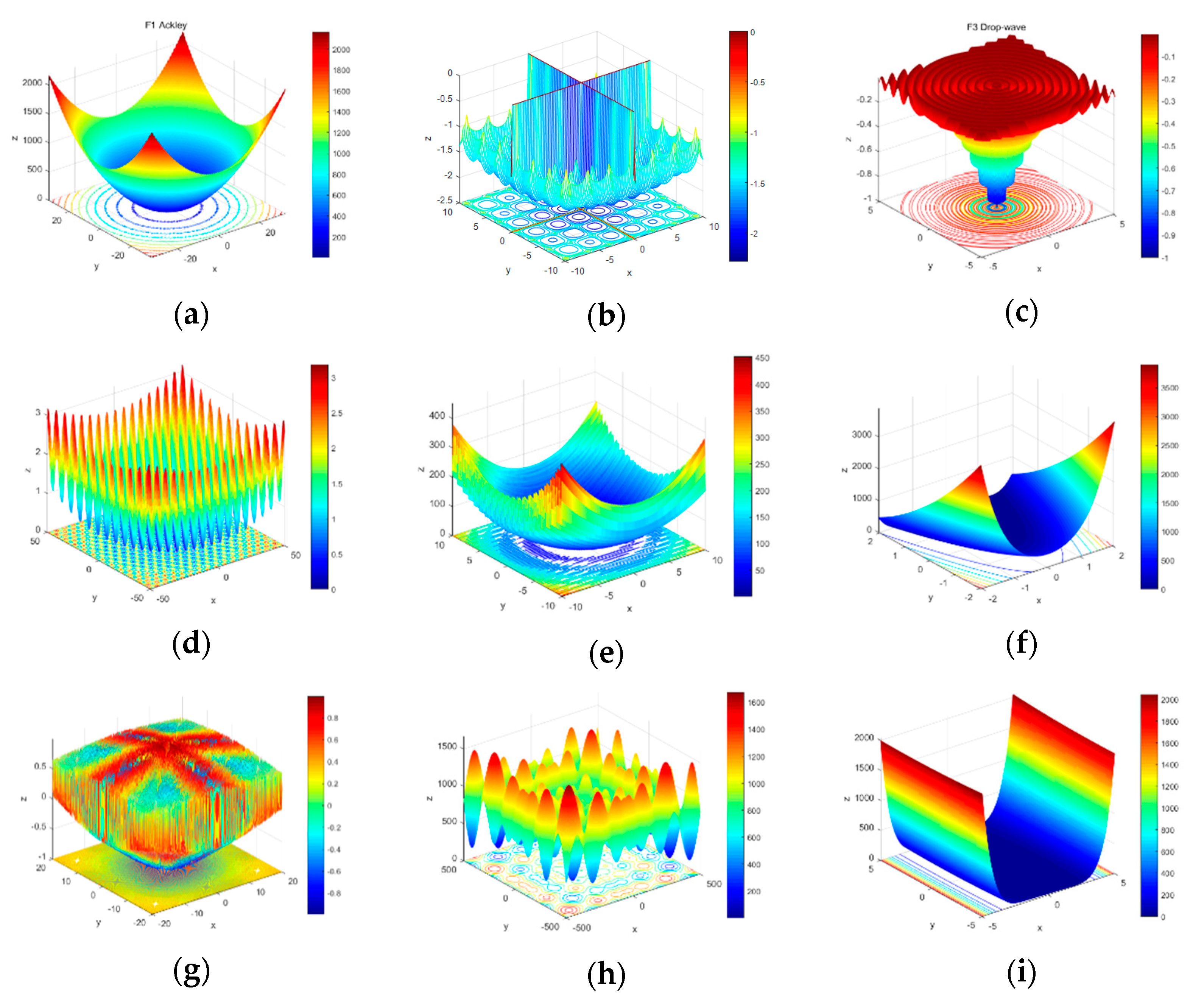
In order to evaluate the performance of the proposed NAIWO algorithm, two simulation experiments were designed and the details of which are provided in this section. In the first part, nine well-known test functions were selected to verify the searching ability of the proposed NAIWO. Table A1 shows the basic information of the nine benchmark functions and the corresponding 2D perspectives are shown in Figure A1.

Table A1.
Two-dimensional benchmark test functions considered in the simulations.
| Functions | Names | Dimension | Solution Range | Global Minimum |
|---|---|---|---|---|
| F1 | Ackley | 2 | fmin = 0 at (0, 0) | |
| F2 | Cross-in-Tray | 2 | fmin = −2.06261 at (±1.3491, ±1.3491) | |
| F3 | Drop-wave | 2 | fmin = −1 at (0, 0) | |
| F4 | Griewank | 2 | fmin = 0 at (0, 0) | |
| F5 | Levy | 2 | fmin = 0 at (1, 1) | |
| F6 | Rosenbrock | 2 | fmin = 0 at (1, 1) | |
| F7 | Schaffer | 2 | fmin = 0 at (0, 0) | |
| F8 | Schwefel | 2 | fmin = 0 at (420.9687, 420.9687) | |
| F9 | Three-hump camel | 2 | fmin = 0 at (0, 0) |
Figure A1.
A two-dimensional perspective with contours of the benchmark test functions, including (a) Ackley function (F1), (b) Cross-in-Tray function (F2), (c) Drop-wave function (F3), (d) Griewank function (F4), (e) Levy function (F5), (f) Rosenbrock function (F6), (g) Schaffer function (F7), (h) Schwefel function (F8), and (i) Three-hump camel function (F9).

Except for F6 and F9, all the other seven functions have a large number of local minimums. Even for F6 and F9, the global minimum of the function cannot be easily found when reaching the convergence point. These functions are widely used in the performance test of any newly proposed intelligent algorithm [25,26].
During the test, the initial search range () of the IWO algorithm and the NAIWO algorithm is generally 1% of the definition domain and the final search range is . The initial population P0 = 25 and the maximum population ; Maximum number of iterations . Where in the NAIWO algorithm, the determination parameters of the niche radius are a = 3, b = 1.05, and k = 0.6, Adaptive spatial diffusion parameter K = 5 and T = 10.
Figure A2 shows the fitness curves of the two algorithms. The maximum number of iterations selected in the test is 300, while the global search of the two algorithms is mainly reflected in the first 100 generations and the iterative process of the latter is mainly local search in order to obtain better convergence accuracy. Therefore, when generating the fitness curve, in order to better display the contrast, the first 100 generations of data were selected. The nine images in Figure A2 illustrate that the NAIWO algorithm proposed in this study has obvious advantages in both global convergence ability and convergence speed than the IWO.
In order to obtain more reliable results, each function was tested 30 times and the average value, minimum value, and variance are shown in Table A2. By comparing the minimum convergence values of the two algorithms in Table A2, it can be seen that in most cases, the NAIWO algorithm has comparable or higher convergence accuracy than the IWO algorithm. Meanwhile, the mean of convergence can better reflect the overall convergence of the algorithm. The analysis reflects that NAIWO has a higher probability of converging to the global minimum than IWO. The variance data shows that the stability of the NAIWO algorithm converging to the global optimal solution is much higher than IWO.
Figure A2.
Comparison of the fitness curves between NAIWO and IWO. The maximum number of iterations selected in the test is 300. In order to better display the contrast, the first 100 generations are selected when generating the image. (a) Ackley function (F1), (b) Cross-in-Tray function (F2), (c) Drop-wave function (F3), (d) Griewank function (F4), (e) Levy function (F5), (f) Rosenbrock function (F6), (g) Schaffer function (F7), (h) Schwefel function (F8), and (i) Three-hump camel function (F9).

Table A2.
Comparison data of IWO and NAIWO algorithms.
| Functions | Algorithms | Mean | Minimum | Variance |
|---|---|---|---|---|
| F1 | IWO | 0.96031 | 1.329 × 10⁻⁷ | 11.153 |
| NAIWO | 1.702 × 10⁻⁶ | 1.4251× 10⁻⁷ | 5.9939 × 10⁻¹³ | |
| F2 | IWO | −2.0511 | −2.0626 | 1.919× 10⁻³ |
| NAIWO | −2.0626 | −2.0626 | 1.2302 × 10⁻²⁸ | |
| F3 | IWO | −0.8402 | −1 | 1.983 × 10⁻² |
| NAIWO | −1 | −1 | 7.125 × 10⁻²⁴ | |
| F4 | IWO | 5.5380 × 10⁻² | 4.6835 × 10⁻² | 2.1 × 10⁻⁴ |
| NAIWO | 1.9692 × 10⁻¹⁴ | 1.22125 × 10⁻¹⁵ | 5.3704 × 10⁻²⁸ | |
| F5 | IWO | 1.895 | 5.7394 × 10⁻¹³ | 5.95262 |
| NAIWO | 2.125 × 10⁻¹² | 1.1457 × 10⁻¹³ | 5.7893 × 10⁻²⁴ | |
| F6 | IWO | 6.29 × 10⁻³ | 3.8735 × 10⁻¹⁴ | 4.1 × 10⁻⁴ |
| NAIWO | 8.3774 × 10⁻¹³ | 7.91675 × 10⁻¹⁶ | 5.876 × 10⁻²⁵ | |
| F7 | IWO | 6.474 × 10⁻³ | 0 | 5.0604 × 10⁻⁵ |
| NAIWO | 6.6613 × 10⁻¹⁷ | 0 | 2.0912 × 10⁻³² | |
| F8 | IWO | 68.431 | 2.5455 × 10⁻⁵ | 7463.60 |
| NAIWO | 7.8959 | 2.5455 × 10⁻⁵ | 902.928 | |
| F9 | IWO | 3.98 × 10⁻² | 1.66 × 10⁻¹⁵ | 1.066 × 10⁻² |
| NAIWO | 1.32 × 10⁻¹³ | 7.04 × 10⁻¹⁶ | 1.229 × 10⁻²⁶ |
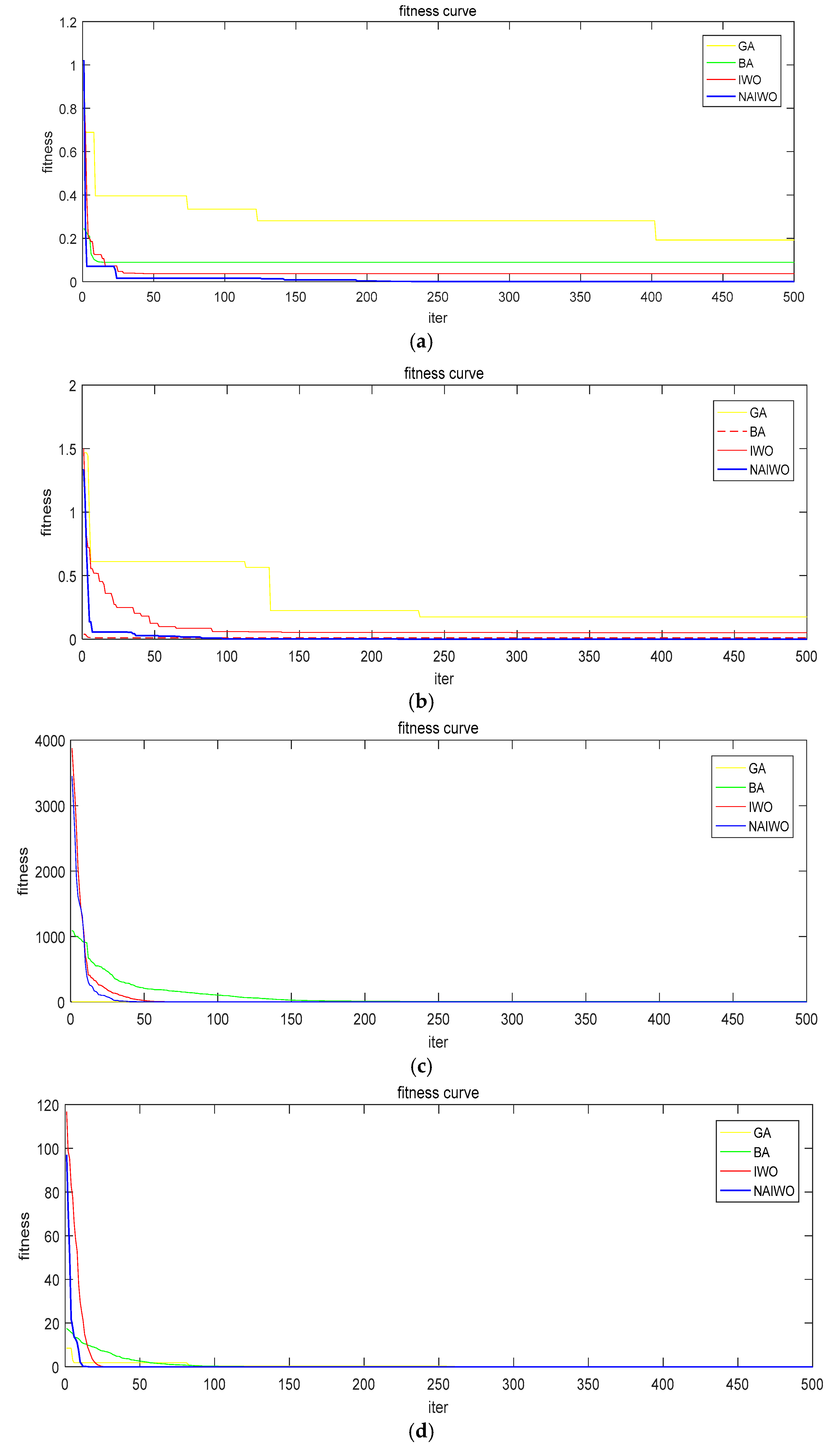
To further verify the optimization ability of the proposed NAIWO algorithm, two well-known optimization algorithms, genetic algorithm (GA) and bat algorithm (BA), are compared using four higher-dimensional benchmark functions in this section. Table A3 shows the details of the four test functions. The number of iterations is 500 and the selection methods of the value of other parameters are the same as above.
Table A3.
High dimensional benchmark test functions considered in the simulations.
| Functions | Names | Dimension | Equations | Global Minimum |
|---|---|---|---|---|
| F10 | Griewank | 3 | fmin = 0 at (0,0,0) | |
| F11 | Rastirgin | 3 | fmin = 0 at (0,0,0) | |
| F12 | Colville | 4 | fmin = 0 at (1,1,1,1) | |
| F13 | Powell | 4 | fmin = 0 at (0,0,0,0) |
Figure A3 shows the fitness curve of the iterative process of the four algorithms, which shows that in the process of finding the minimum value of F10 and F11 functions, the NAIWO algorithm has the most outstanding comprehensive convergence ability and fastest convergence speed. BA also has a faster convergence speed, but its poor convergence stability makes it possible to converge to a local minimum with a certain probability.
The statistical information of the 30 repeated simulations shown in Table A4 also confirms the conclusions made above. In the 30 runs of the two functions F10 and F11, the minimum convergence accuracy of the BA algorithm is the highest of the four algorithms, but its average value and variance value are higher than that of the NAIWO algorithm by one or more orders of magnitude, indicating that its convergence probability and stability are far inferior to the NAIWO algorithm. The comparison of the statistical data of F10–F13 shows that the NAIWO algorithm has greater advantages in stability and convergence accuracies compared with the other three algorithms, which shows the effectiveness of the proposed algorithm.
Figure A3.
Comparison of the fitness curves between NAIWO, IWO, GA, and BA. The maximum number of iterations selected in the test is 500. (a) Griewank function (F10), (b) Rastirgin function (F11), (c) Colville function (F12), and (d) Powell function (F13).
Figure A3.
Comparison of the fitness curves between NAIWO, IWO, GA, and BA. The maximum number of iterations selected in the test is 500. (a) Griewank function (F10), (b) Rastirgin function (F11), (c) Colville function (F12), and (d) Powell function (F13).

Table A4.
Statistical comparison data of IWO, GA, BA, and NAIWO algorithms.
| Functions | Algorithms | Mean | Minimum | Variance |
|---|---|---|---|---|
| F10 | IWO | 1.45927 | 2.58225 × 10⁻¹⁰ | 1.27896 |
| GA | 0.42361 | 0.02378 | 0.17285 | |
| BA | 0.43115 | 2.70894 × 10⁻¹² | 0.25147 | |
| NAIWO | 2.3897 × 10⁻⁹ | 6.7921 × 10⁻¹¹ | 3.5773 × 10⁻¹⁸ | |
| F11 | IWO | 0.18875 | 0.00740 | 0.01780 |
| GA | 0.35222 | 0.08101 | 0.01243 | |
| BA | 0.01052 | 8.88178 × 10⁻¹⁴ | 0.00023 | |
| NAIWO | 0.00263 | 1.61982 × 10⁻¹³ | 1.71477 × 10⁻⁵ | |
| F12 | IWO | 0.25676 | 1.02182 × 10⁻¹⁰ | 0.39066 |
| GA | 0.19600 | 0.01125 | 0.02123 | |
| BA | 1.77976 | 0.01474 | 3.29279 | |
| NAIWO | 0.00011 | 4.29174 × 10⁻¹¹ | 1.66852 × 10⁻⁷ | |
| F13 | IWO | 1.73784 × 10⁻⁷ | 1.98073 × 10⁻¹² | 3.33946 × 10⁻¹³ |
| GA | 0.08609 | 0.00225 | 4.89659 × 10⁻³ | |
| BA | 8.79407 × 10⁻⁵ | 7.17666 × 10⁻⁶ | 5.63957 × 10⁻⁹ | |
| NAIWO | 1.63239 × 10⁻⁹ | 1.12409 × 10⁻¹² | 1.03073 × 10⁻¹⁷ |
Appendix B
ASM1 contains 13 substrate components (seven soluble components and six insoluble components) as shown in Table A5. The influent concentrations of these 13 components reflects the degree of contamination of the influent to the wastewater treatment plant. All the 13 substrates have their reaction rates and the reaction rate equations are given in Table A6.
Table A5.
The 13 components of ASM1.
| Components | Definition | Unit |
|---|---|---|
| SI | Soluble inert organic matter | g∙COD∙m−3 |
| SS | Readily biodegradable substrate | g∙COD∙m−3 |
| XI | Particulate inert organic matter | g∙COD∙m−3 |
| XS | Slowly biodegradable substrate | g∙COD∙m−3 |
| XB,H | Active heterotrophic biomass | g∙COD∙m−3 |
| XB,A | Active autotrophic biomass | g∙COD∙m−3 |
| XP | Particulate product arising from biomass decay | g∙COD∙m−3 |
| SO | Oxygen (negative COD) | g∙COD∙m−3 |
| SNO | Nitrate and nitrite nitrogen | g∙N∙m−3 |
| SNH | NH4+ and NH3 nitrogen | g∙N∙m−3 |
| SND | Soluble biodegradable organic nitrogen | g∙N∙m−3 |
| XND | Particulate biodegradable organic nitrogen | g∙N∙m−3 |
| SALK | Alkalinity | mol∙m−3 |
Table A6.
Reaction rate equations of the 13 components.
| Components | Reactions |
|---|---|
| SI (i = 1) | |
| SS (i = 2) | |
| XI (i = 3) | |
| XS (i = 4) | |
| XB,H (i = 5) | |
| XB,A (i = 6) | |
| XP (i = 7) | |
| SO (i = 8) | |
| SNO (i = 9) | |
| SNH (i = 10) | |
| SND (i = 11) | |
| XND (i = 12) | |
| SALK (i = 13) |
Table A7.
Reaction rate of eight sub-reaction processes.
| Processes | Descriptions |
|---|---|
References
- Henze, M.; Grady, L., Jr.; Gujer, W.; Marais, G.; Matsuo, T. Activated Sludge Model No. 1; IAWPRC: London, UK, 1987; Available online: https://www.researchgate.net/publication/243624144_Activated_Sludge_Model_No_1 (accessed on 15 September 2020).
- Al Madany, A.M.; El-Seddik, M.M.; Abdallah, K.Z. Extended Activated Sludge Model No. 1 with Floc and Biofilm Diffusion for Organic and Nutrient Removal. J. Environ. Eng. 2020, 146, 04020008. [Google Scholar] [CrossRef]
- Salles, N.A.; de Souza, T.S.O. Activated Sludge Model No. 1 (ASM1) applicability for simulation of sanitary sewage and landfill leachate co-treatment in aerated lagoons. Eng. Sanit. Ambient. 2020, 25, 293–301. [Google Scholar] [CrossRef] [Green Version]
- Hauduc, H.; Gillot, S.; Rieger, L.; Ohtsuki, T.; Shaw, A.; Takács, I.; Winkler, S. Activated sludge modelling in practice: An international survey. Water Sci. Technol. 2009, 60, 1943–1951. [Google Scholar] [CrossRef] [PubMed]
- Van Loosdrecht, M.C.M.; Lopez-Vazquez, C.M.; Meijer, S.; Hooijmans, C.M.; Brdjanovic, D. Twenty-five years of ASM1: Past, present and future of wastewater treatment modelling. J. Hydroinform. 2015, 17, 697–718. [Google Scholar] [CrossRef] [Green Version]
- Hauduc, H.; Rieger, L.; Oehmen, A.; Van Loosdrecht, M.C.M.; Comeau, Y.; Héduit, A.; Vanrolleghem, P.; Gillot, S. Critical review of activated sludge modeling: State of process knowledge, modeling concepts, and limitations. Biotechnol. Bioeng. 2012, 110, 24–46. [Google Scholar] [CrossRef]
- Bhuyan, S.; Koelliker, J.; Marzen, L.; Harrington, J. An integrated approach for water quality assessment of a Kansas watershed. Environ. Model. Softw. 2003, 18, 473–484. [Google Scholar] [CrossRef]
- Yeh, W.W.-G.; Yoon, Y.S.; Lee, K.S. Aquifer parameter identification with kriging and optimum parameterization. Water Resour. Res. 1983, 19, 225–233. [Google Scholar] [CrossRef]
- Ratto, M.; Tarantola, S.; Saltelli, A. Sensitivity analysis in model calibration: GSA-GLUE approach. Comput. Phys. Commun. 2001, 136, 212–224. [Google Scholar] [CrossRef]
- Omlin, M.; Reichert, P. A comparison of techniques for the estimation of model prediction uncertainty. Ecol. Model. 1999, 115, 45–59. [Google Scholar] [CrossRef]
- Beven, K.; Binley, A. The future of distributed models: Model calibration and uncertainty prediction. Hydrol. Process. 1992, 6, 279–298. [Google Scholar] [CrossRef]
- Cho, J.; Sung, K.S.; Ha, S.R. A river water quality management model for optimising regional wastewater treatment using a genetic algorithm. J. Environ. Manag. 2004, 73, 229–242. [Google Scholar] [CrossRef] [PubMed]
- Miró, A.; Pozo, C.; Guillén-Gosálbez, G.; Egea, J.A.; Jiménez, L. Deterministic global optimization algorithm based on outer approximation for the parameter estimation of nonlinear dynamic biological systems. BMC Bioinform. 2012, 13, 90. [Google Scholar] [CrossRef] [PubMed] [Green Version]
- Gandomi, A.H.; Yang, X.S.; Talatahari, S.; Alavi, A.H. (Eds.) Metaheuristic Applications in Structures and Infrastructures; Elsevier Science Publishers B.V.: Amsterdam, The Netherlands, 2013. [Google Scholar]
- Kim, S.; Lee, H.; Kim, J.; Kim, C.; Ko, J.; Woo, H.; Kim, S. Genetic algorithms for the application of Activated Sludge Model No. 1. Water Sci. Technol. 2002, 45, 405–411. [Google Scholar] [CrossRef] [PubMed]
- Du, X.; Wang, J.; Jegatheesan, V.; Shi, G. Parameter estimation of activated sludge process based on an improved cuckoo search algorithm. Bioresour. Technol. 2018, 249, 447–456. [Google Scholar] [CrossRef]
- Mehrabian, A.; Lucas, C. A novel numerical optimization algorithm inspired from weed colonization. Ecol. Inform. 2006, 1, 355–366. [Google Scholar] [CrossRef]
- Wu, H.; Liu, C.; Xie, X. Pattern synthesis of planar antenna arrays based on invasive weed optimization algorihm. J. Naval Univ. Eng. 2015, 27, 16–19. [Google Scholar]
- Liu, Y.; Jiao, Y.-C.; Zhang, Y.-M. A novel hybrid invasive weed optimization algorithm for pattern synthesis of array antennas. Int. J. RF Microw. Comput. Aided Eng. 2014, 25, 154–163. [Google Scholar] [CrossRef]
- Duan, M.; Yuan, C. Fault diagnosis of nuclear power plant based on invasive weed optimization algorithm. At. Energy Sci. Technol. 2015, 49, 719–724. [Google Scholar]
- Cuevas, E.; Rodríguez, A.; Valdivia, A.; Zaldívar, D.; Pérez, M. A hybrid evolutionary approach based on the invasive weed optimization and estimation distribution algorithms. Soft Comput. 2019, 23, 13627–13668. [Google Scholar] [CrossRef]
- Martins, T.M.; Neves, R.F. Applying genetic algorithms with speciation for optimization of grid template pattern detection in financial markets. Expert Syst. Appl. 2020, 147, 113191. [Google Scholar] [CrossRef]
- Zhou, S.J.; Li, H.M.; Gao, T.B. Combination of Ant Algorithm and niche Genetic Algorithm. In Proceedings of First International Conference of Modelling and Simulation, Volume IV: Modelling and Simulation in Business, Management, Economic and Finance; Yu, H.G., Jiang, Y., Eds.; World Academic Union-World Academic Press: Liverpool, UK, 2008; pp. 169–172. [Google Scholar]
- Mirjalili, S.; Mirjalili, S.M.; Lewis, A. Grey Wolf Optimizer. Adv. Eng. Softw. 2014, 69, 46–61. [Google Scholar] [CrossRef] [Green Version]
- Ju, X.; Peng, D. Kinetic parameters sensitivity analysis of model ASM1. Environ. Sci. Technol. 2010, 33, 312–314. [Google Scholar]
- Faramarzi, A.; Heidarinejad, M.; Stephens, B.; Mirjalili, S. Equilibrium optimizer: A novel optimization algorithm. Knowl. Based Syst. 2020, 191, 105190. [Google Scholar] [CrossRef]
Figure 1.
Schematic diagram of activated sludge model 1 (ASM1) parameter estimation using the niche-based adaptive invasive weed optimization (NAIWO) algorithm.
Figure 1.
Schematic diagram of activated sludge model 1 (ASM1) parameter estimation using the niche-based adaptive invasive weed optimization (NAIWO) algorithm.

Figure 2.
Basic processing blocks of the activated sludge process based wastewater treatment plants.
Figure 2.
Basic processing blocks of the activated sludge process based wastewater treatment plants.

Figure 3.
Flow chart of the NAIWO algorithm used in ASM1 parameter estimation.

Figure 4.
The fitness curves of four algorithms produced during the parameter estimation for (a) Pingliang City Wastewater Treatment Plant (PC-WWTP) and (b) WC-WWTP.
Figure 4.
The fitness curves of four algorithms produced during the parameter estimation for (a) Pingliang City Wastewater Treatment Plant (PC-WWTP) and (b) WC-WWTP.

Figure 5.
Comparison of predicted and measured values of effluent water quality parameters for (a) Ammonia nitrogen (SNH), (b) nitrate nitrogen (SNO), (c) soluble rapidly biodegradable organic matter (SS), and (d) insoluble slowly degradable organic matter (XS) in PC-WWTP.
Figure 5.
Comparison of predicted and measured values of effluent water quality parameters for (a) Ammonia nitrogen (SNH), (b) nitrate nitrogen (SNO), (c) soluble rapidly biodegradable organic matter (SS), and (d) insoluble slowly degradable organic matter (XS) in PC-WWTP.

Figure 6.
Comparison of predicted and measured values of effluent water quality parameters for (a) Ammonia nitrogen (SNH), (b) nitrate nitrogen (SNO), (c) soluble rapidly biodegradable organic matter (SS), and (d) insoluble slowly degradable organic matter (XS) in WC-WWTP.
Figure 6.
Comparison of predicted and measured values of effluent water quality parameters for (a) Ammonia nitrogen (SNH), (b) nitrate nitrogen (SNO), (c) soluble rapidly biodegradable organic matter (SS), and (d) insoluble slowly degradable organic matter (XS) in WC-WWTP.

Table 1.
Nineteen parameters of ASM1.
| Symbol | Description | Value ++ | Unit |
| 5 stoichiometric parameters | |||
| YA | Yield coefficient of autotrophic bacteria | 0.24 | g cell COD formed·(g COD oxidized)−1 |
| YH | Heterotrophic yield coefficient | 0.67 | g cell COD formed·(g N oxidized)−1 |
| fp | Proportion of inert particles in microorganisms | 0.08 | dimensionless |
| ixb | Proportion of nitrogen content in microbial cells | 0.086 | g N·(g COD)−1 in biomass |
| ixp | Proportion of nitrogen content in microbial products | 0.06 | g N·(g COD)−1 in particulate products |
| 14 kinetic parameters | |||
| Maximum specific growth rate coefficient of heterotrophic bacteria | 6.0 | d−1 | |
| KS | Half saturation coefficient of heterotrophic bacteria | 20.0 | g COD·m−3 |
| KO,H | Oxygen half-saturation coefficient of heterotrophic bacteria | 0.2 | g COD·m−3 |
| KNO | Nitrate half-saturation coefficient of denitrifying bacteria | 0.5 | g NO3-N·m−3 |
| bH | Attenuation coefficient of heterotrophic bacteria | 0.62 | d−1 |
| Hypoxia correction factor for heterotrophic bacteria under hypoxia | 0.8 | dimensionless | |
| Correction factor for hydrolysis under anoxic conditions | 0.4 | dimensionless | |
| kh | Maximum specific hydrolysis rate | 3.0 | g slowly biodegradable COD·(g cell COD·d)−1 |
| KX | Half saturation coefficient of slowly biodegradable substrate hydrolysis | 0.03 | g slowly biodegradable COD·(g cell COD)−1 |
| Maximum specific growth rate of autotrophic bacteria | 0.80 | d−1 | |
| KNH | Ammonia half-saturation coefficient of autotrophic bacteria | 1.0 | g NH3-N·m−3 |
| KO,A | Oxygen half saturation coefficient of autotrophic bacteria | 0.4 | d−1 |
| ka | Dissolved organic ammonia nitrating rate | 0.08 | g COD·m−3 |
| bA | Autotrophic bacteria specific decay rate | 0.05 | m3·(g COD·d)−1 |
++ The values are for 20 °C, extracted from [1].
Table 2.
Estimated results of seven parameters of ASM1 for PC-WWTP.
| Parameter | Range | International Water Association (IWA) Recommendation (20 °C) | Values Estimated by Selected Algorithms | |||
|---|---|---|---|---|---|---|
| Genetic Algorithm (GA) | Bat Algorithm (BA) | Invasive Weed Optimization (IWO) | NAIWO | |||
| YH | 0.4–0.9 | 0.67 | 0.6663 | 0.6720 | 0.6649 | 0.6690 |
| bH | 0.3–1.2 | 0.62 | 0.3448 | 0.3728 | 0.4413 | 0.4521 |
| µH | 2–18 | 6 | 2.6388 | 2.8941 | 3.2101 | 4.9771 |
| µA | 0.3–2.4 | 0.8 | 0.7293 | 0.9243 | 0.9225 | 0.6733 |
| KOA | 0.13–1.2 | 0.4 | 0.2189 | 0.6011 | 1.1064 | 0.5139 |
| KNH | 0.3–3 | 1 | 1.9232 | 2.0819 | 1.2479 | 1.0908 |
| KS | 10–40 | 20 | 12.9502 | 13.6463 | 13.1019 | 21.8191 |
Table 3.
Estimated results of seven parameters of ASM1 for Wushan County Wastewater Treatment Plant (WC-WWTP).
Table 3.
Estimated results of seven parameters of ASM1 for Wushan County Wastewater Treatment Plant (WC-WWTP).
| Parameter | Range | IWA Recommendation (20 °C) | Values Estimated by Selected Algorithms | |||
|---|---|---|---|---|---|---|
| GA | BA | IWO | NAIWO | |||
| YH | 0.4–0.9 | 0.67 | 0.7630 | 0.7447 | 0.7247 | 0.7510 |
| bH | 0.3–1.2 | 0.62 | 0.4953 | 0.5480 | 0.5482 | 0.5891 |
| µH | 2–18 | 6 | 4.9608 | 5.7496 | 8.5081 | 6.2899 |
| µA | 0.3–2.4 | 0.8 | 2.2481 | 1.4434 | 1.9918 | 0.9003 |
| KOA | 0.13–1.2 | 0.4 | 1.1205 | 0.5600 | 1.1855 | 0.3851 |
| KNH | 0.3–3 | 1 | 2.8231 | 1.9352 | 1.9732 | 1.0687 |
| KS | 10–40 | 20 | 18.2024 | 16.8986 | 28.1369 | 18.8017 |
© 2020 by the authors. Licensee MDPI, Basel, Switzerland. This article is an open access article distributed under the terms and conditions of the Creative Commons Attribution (CC BY) license (http://creativecommons.org/licenses/by/4.0/).
Share and Cite
MDPI and ACS Style
Du, X.; Ma, Y.; Wei, X.; Jegatheesan, V. Optimal Parameter Estimation in Activated Sludge Process Based Wastewater Treatment Practice. Water 2020, 12, 2604. https://doi.org/10.3390/w12092604
AMA Style
Du X, Ma Y, Wei X, Jegatheesan V. Optimal Parameter Estimation in Activated Sludge Process Based Wastewater Treatment Practice. Water. 2020; 12(9):2604. https://doi.org/10.3390/w12092604
Chicago/Turabian StyleDu, Xianjun, Yue Ma, Xueqin Wei, and Veeriah Jegatheesan. 2020. "Optimal Parameter Estimation in Activated Sludge Process Based Wastewater Treatment Practice" Water 12, no. 9: 2604. https://doi.org/10.3390/w12092604
Note that from the first issue of 2016, this journal uses article numbers instead of page numbers. See further details here.