The Impacts of the COVID-19 Lockdown on Air Quality in the Guanzhong Basin, China


1
College of Geological Engineering and Geomatics, Chang’an University, Xi’an 710054, China
2
Royal Netherlands Meteorological Institute (KNMI), R&D Satellite Observations, 3731GA De Bilt, The Netherlands
3
Institute of Remote Sensing and Digital Earth, Chinese Academy of Sciences, Beijing 100101, China
*
Author to whom correspondence should be addressed.
Remote Sens. 2020, 12(18), 3042; https://doi.org/10.3390/rs12183042
Submission received: 10 August 2020
/
Revised: 11 September 2020
/
Accepted: 15 September 2020
/
Published: 17 September 2020
(This article belongs to the Section Atmospheric Remote Sensing)
Abstract
:The Corona Virus Disease 2019 (COVID-19) appeared in Wuhan, China, at the end of 2019, spreading from there across China and within weeks across the whole world. In order to control the rapid spread of the virus, the Chinese government implemented a national lockdown policy. It restricted human mobility and non-essential economic activities, which, as a side effect, resulted in the reduction of the emission of pollutants and thus the improvement of the air quality in many cities in China. In this paper, we report on a study on the changes in air quality in the Guanzhong Basin during the COVID-19 lockdown period. We compared the concentrations of PM2.5, PM10, SO2, NO2, CO and O3 obtained from ground-based monitoring stations before and after the COVID-19 outbreak. The analysis confirmed that the air quality in the Guanzhong Basin was significantly improved after the COVID-19 outbreak. During the emergency response period with the strictest restrictions (Level-1), the concentrations of PM2.5, PM10, SO2, NO2 and CO were lower by 37%, 30%, 29%, 52% and 33%, respectively, compared with those before the COVID-19 outbreak. In contrast, O3 concentrations increased substantially. The changes in the pollutant concentrations varied between cities during the period of the COVID-19 pandemic. The highest O3 concentration changes were observed in Xi’an, Weinan and Xianyang city; the SO2 concentration decreased substantially in Tongchuan city; the air quality had improved the most in Baoji City. Next, to complement the sparsely distributed air quality ground-based monitoring stations, the geographic and temporally weighted regression (GTWR) model, combined with satellite observations of the aerosol optical depth (AOD) and meteorological factors was used to estimate the spatial and temporal distributions of PM2.5 and PM10 concentrations with a resolution of 6 km × 6 km before and after the COVID-19 outbreak. The model was validated by a comparison with ground-based observations from the air quality monitoring network in five cities in the Guanzhong Basin with excellent statistical metrics. For PM2.5 and PM10 the correlation coefficients R2 were 0.86 and 0.80, the root mean squared errors (RMSE) were 11.03 µg/m3 and 14.87 µg/m3 and the biases were 0.19 µg/m3 and −0.27 µg/m3, which led to the conclusion that the GTWR model could be used to estimate the PM concentrations in locations where monitoring data were not available. Overall, the PM concentrations in the Guanzhong Basin decreased substantially during the lockdown period, with a strong initial decrease and a slower one thereafter, although the spatial distributions remained similar.

1. Introduction
China informed the World Health Organization (WHO) of several rare pneumonia cases in Wuhan, Hubei Province, on 31 December of 2019 [1], caused by a novel corona virus called SARS-CoV-2. On 12 February 2020, the WHO named this pneumonia Corona Virus Disease 2019 (COVID-19) (http://www.euro.who.int/en/health-topics/health-emergencies/novel-coronavirus-2019-ncov_old, last access 11 September 2020). Some early studies had shown that possible ways of transmission of the virus were through respiratory droplets transmitted over short distances when people were in close contact [2], therefore human-to-human contact could increase the risk of COVID-19 infection [3]. In addition, research showed that COVID-19 infection could also be transmitted through aerosols [4]. The number of COVID-19 cases exceeded 27 million globally with a total death toll of about 900 thousand in more than 200 countries (regions) as of 6 September 2020 (https://www.who.int/emergencies/diseases/novel-coronavirus-2019/situation-reports, last access 11 September 2020).
There is evidence that pollutants are closely related to the increased risk of various diseases, especially severe viral respiratory disease [5,6]. According to the data from the WHO, 4.3 million people die each year from diseases directly related to poor air quality [7]. Among them, respiratory and cardiovascular diseases caused by particulate matter with aerodynamic diameter less than or equal to 2.5µm (PM2.5) or 10µm (PM10) are prominent, and they can even increase mortality [8,9]. Additionally, trace gases like sulfur dioxide (SO2), nitrogen dioxide (NO2), carbon oxide (CO) and ozone (O3) could also enter the respiratory tract through respiration and aggravate the susceptibility and severity of a respiratory virus infection [10]. Severe outbreak of COVID-19 occurred in the areas with high pollution levels and evidence of the influence of air pollution on COVID-19 infections were reported [11,12]. People exposed to high levels of particulate matter are more prone to get infected by the SARS-CoV-2 virus, with increased mortality [13].
In order to control the spread of COVID-19, policy measures were implemented in many countries, with many restrictions and even complete lockdowns. The Chinese government established emergency response procedures from late January 2020 [14,15]. The COVID-19 outbreak in Wuhan led to a complete lockdown of the city on the 23 of January 2020, just before the Spring Festival, the most important traditional festival in China, which in 2020 was on the 25 of January. This lockdown reduced traffic, commerce, construction and industry to essential only, and people were confined to their homes. Although the implementation of these preventive measures has brought significant economic costs, it could also be used as a unique experiment to assess the influence of large-scale emission reduction on air quality [16]. Satellite images of the National Aeronautics and Space Administration (NASA) clearly showed that the NO2 concentration in China dropped significantly after the lockdown and the reduction of NO2 pollution was first apparent near Wuhan city, then spread to the whole country (https://earthobservatory.nasa.gov/images/146362/airborne-nitrogen-dioxide-plummets-over-china, last access 11 September 2020). Several studies showed that the concentrations of major pollutants such as PM2.5, PM10, SO2, NO2 and CO decreased significantly in China, although in response to the reduced NO2 concentrations those of O3 increased [17,18]. Similar studies in other countries, such as in Europe, Asia and North America, also showed a significant decrease in air pollution levels in many cities after the implementation of the measures to avoid spreading COVID-19 [19,20,21].
Many studies were already published on the effect of the measures to prevent spreading COVID-19 on air quality in China. Among these, [22] studied the change in the concentrations of six pollutants (PM2.5, PM10, SO2, NO2, CO, O3) one month before and after the COVID-19 lockdown in Wuhan city. Furthermore, [23] studied the impact of the COVID-19 outbreak on the air quality index near Central China cities (Anqing, Hefei and Suzhou) from January to March 2020. Moreover, [18] reported the impact of human activity pattern changes on air pollution variation during the COVID-19 lockdown over the Yangtze River Delta Region from 1 January to 17 April 2020. Regional air quality indicators were investigated by [24] over the Beijing-Tianjin-Hebei region and other parts of China during the winter from November 2019 to February 2020 to study the effects of the COVID-19 outbreak in China. The NOx emission reduction and recovery during COVID-19 in East China from 1 January to 12 March were presented by [25]. Furthermore, [17] researched the impact of the control measures during the COVID-19 outbreak on air pollution in China for the period of 30 days before and after the Spring Festival, based on a comparison with the three preceding years, using both satellite and ground-based data. The Guanzhong Basin (GZB), located in Shaanxi Province (see Figure 1), is the most economically developed area in northwest China and its serious long-term air pollution has become a focus issue in China [26]. As an enclosed region, the geographical condition of the basin surrounded by high mountains leads to stagnant air and a low wind speed in the valley, which results in the accumulation of pollutants. These meteorological conditions play a key role in the formation, transformation, diffusion, migration and removal of air pollutants [27]. Since the outbreak of COVID-19, Shaanxi Province, which is adjacent to Hubei Province, has also actively responded to the lockdown policy and achieved good results in the prevention and control of the epidemic. The effects of these measures on the air quality in this special enclosed region are reported in this study. Pollutants measured at ground-based monitoring stations in the GZB area (PM2.5, PM10, SO2, NO2, CO and O3) during the periods before and after the COVID-19 outbreak are compared and analyzed in detail. In addition, different than other studies, our study covered the period from 1 January to 31 August 2020, i.e., including the period before the COVID-19 outbreak, the lockdown stage, the pandemic stage and the control stage in China to comprehensively and systematically explore the impact of COVID-19 on air quality.
Another difference from previous studies is that we not only compared and analyzed concentrations of pollutants that are routinely measured at the ground-based monitoring stations, but also used a model together with satellite observations to estimate the near-surface PM2.5 and PM10 concentrations with a resolution of 6 km × 6 km over the entire Guanzhong Basin area. This model estimates the complement sparsely distributed air quality ground-based monitoring stations and is used to explore spatial and temporal changes of PM concentrations with high spatial resolution during the period of COVID-19 pandemic. The model uses aerosol optical depth (AOD) from the Visible Infrared Imaging Radiometer Suite (VIIRS) satellite. AOD is the column-integrated aerosol extinction coefficient, which can be used as a proxy for the particulate matter concentration in the atmospheric column and the degree of air pollution [28]. However, the PM–AOD relationship depends on meteorological factors (such as planetary boundary layer height, relative humidity, wind speed and temperature) that need to be accounted for when PM concentrations are derived from satellite AOD measurements [29]. The normalized difference vegetation index (NDVI) could be used as another independent variable to predict the PM concentration [30]. AOD measured from satellites has been widely used together with statistical models, such as a linear mixed effects model [31], a geographically weighted regression model [30] or a random forests machine learning model [32] to estimate particulate matter (PM) concentrations. In this study, the geographic and temporally weighted regression (GTWR) model [33] was used to evaluate both the spatial and temporal variability of PM based on satellite observations of AOD with meteorological factors and NDVI data.
The National Emergency Response Plan for Public Emergencies issued by the State Council of China (http://www.scio.gov.cn/xwfbh/zdjs/Document/1078861/1078861.htm, last access 11 September 2020) classifies public emergencies into four levels: 1st level (especially serious), 2nd level (serious), 3rd level (heavy) and 4th level (general). Following this classification, we divided the whole research period into six stages to get insight into the effects of the various measures on the air quality in the study area: the stage before the COVID-19 lockdown is the Pre-lockdown stage (1–24 January 2020). The first-level emergency response phase for public health incidents launched by the Shaanxi Province is the Level-1 stage (25 January–27 February 2020). The transition between the 1st level and the 3rd level emergency response phase is the Level-2 stage (27 February–26 March 2020). The COVID-19 measures in Shaanxi Province were relaxed from 27 March 2020, and the period until April 30 is the Level-3 stage (27 March–30 April 2020). The Level-4 and Level-5 stages cover the period from 1 May until 31 August 2020. It is split into two stages because the VIIRS AOD data were only available until 24 June 2020, which determines the Level-4 stage (1 May–24 June 2020). The Level-5 stage is from 24 June until the end of the study period, i.e., 24 June–31 August 2020.
2. Data and Methods
2.1. Study Area
The Guanzhong Basin (GZB) is located in the central part of Shaanxi Province (Figure 1). There are 54 cities and districts in the Guanzhong Basin, including five prefecture-level cities (second level administrative divisions of China, Xi’an, Xianyang, Tongchuan, Baoji and Weinan). It is a region distributed in the urban cluster of Shaanxi, with a total area of 55,623 km2. GZB is the Weihe River alluvial plain with an average altitude of about 500 m. The basin is surrounded by the Qinling Mountains to the south and the Loess Plateau to the north. The mountains form a natural barrier around the Guanzhong Basin which prevents the transport of air pollutants out of the basin resulting in their accumulation. The air pollution in this area is serious due to dense population, the concentration of urban agglomerations and a large number of boilers and coal burning used in the winter heating period [27,34,35]. According to the Environmental Status Bulletin of Shaanxi Province in 2019, the air pollutants in the Guanzhong Basin area are mainly PM2.5 and PM10 and the air quality is lightly polluted or above on nearly 40% of the days throughout the whole year (http://sthjt.shaanxi.gov.cn/newstype/hbyw/hjzl/hjzkgb/20200604/55508.html, last access 11 September 2020).
2.2. Data
2.2.1. Ground-Based Air Quality Data
The hourly concentrations of air pollutants were collected from the ground-based observations freely available from China’s National Environmental Monitoring Center (CNEMC, http://www.cnemc.cn, last access 11 September 2020). Previous studies have shown the statistical reliability of the CNEMC data [36,37]. The data include PM2.5, PM10, SO2, NO2, CO and O3. For the current study, hourly concentrations of these species were collected from 33 air quality stations (shown in Figure 1) in five cities during the same period (1 January to 31 August) in each year from 2017 to 2020. Invalid data due to equipment failure (recorded with the value NA) were deleted. The daily mean concentration in each city was calculated by averaging hourly concentrations at all stations in that city (13 in Xi’an, 4 in Xianyang, 4 in Weinan, 4 in Tongchuan and 8 in Baoji) to represent the citywide pollution exposure condition.
2.2.2. Satellite Data
Suomi National Polar-orbiting Partnership (S-NPP) is the first of a new generation of earth observation satellites launched by the USA to replace the previous generation whose service life was about to expire. S-NPP is a polar orbiting satellite with a daytime overpass time at about 13:30 local solar time (LST). S-NPP is equipped with five optical sensors, including the Visible Infrared Imaging Radiometer Suite (VIIRS) [38]. VIIRS is an environmental remote sensing sensor which provides, among others, cloud cover and aerosol characteristics [39] with daily global coverage. Environmental data record (EDR) is the official VIIRS level 2 product with AOD at 11 wavelengths (0.412, 0.445, 0.488, 0.55, 0.555, 0.672, 0.746, 0.865, 1.24, 1.61 and 2.25 μm) with a spatial resolution of 6 km [39]. VIIRS_EDR provides four different pixel-level quality assurance (QA) flags: not produced (QA = 0), low quality (QA = 1), medium quality (QA = 2) and high quality (QA = 3) (https://www.star.nesdis.noaa.gov/smcd/emb/viirs_aerosol/documents/Aerosol_Product_Users_Guide_V2.0.1.pdf, last access 11 September 2020). [35] evaluated the VIIRS EDR AOD product with QA = 2 and QA = 3 over the Guanzhong Basin by comparing with ground-based AOD measurements in Xi’an, part of the Sun-sky radiometer Observation NETwork (SONET) [40]. The results showed that the use of VIIRS AOD with QA = 3 provides much better accuracy than using AOD with QA = 2. Therefore, VIIRS EDR AOD data at 550 nm wavelength with QA = 3 (https://www.bou.class.noaa.gov/saa/products/welcome, last access 11 September 2020) over the GZB were collected for the study period from 1 January to 24 June 2020 (data after 24 June 2002 were not available at the time of this study). It is noted that VIIRS retrieval fails in some conditions, such as in the presence of clouds, ephemeral water bodies, high reflectance of surfaces covered with snow or ice, or a combination of multiple factors [41], which is a serious problem. Figure 2 illustrates the spatial coverage of VIIRS AOD with QA = 3 during the study period (1 January–24 June 2020). The AOD coverage is mainly between 10–30%.
The other satellite product that was used in this study was the NDVI (Normalized Difference Vegetation Index, unitless). NDVI data are available from the Moderate Resolution Imaging Spectroradiometer (MODIS). It is a Level 3 product with a spatial resolution of 250 m × 250 m and a time resolution of 16 days (product code MOD13Q1) which can be downloaded from https://modis.gsfc.nasa.gov/data/dataprod/mod13.php (last access 11 September 2020).
2.2.3. Meteorological Data
The meteorological data over the study area for the period from 1 January to 24 June 2020 were derived from the latest version ERA5 data from the European Centre for Medium-Range Weather Forecasts (ECMWF) (https://cds.climate.copernicus.eu, last access 11 September 2020). The ERA5 replaced the ERA-Interim re-analysis data which stopped on 31 August 2019. The ERA5 dataset contains hourly atmospheric, terrestrial and oceanic climate variables since 1950 with a spatial resolution of 0.25°. Air temperature (TP, °C), relative humidity (RH, %), planetary boundary layer height (PBLH, m) and wind speed vector into meridional component wind speed U (WSU, m/s) at 13:00 and 14:00 local time (i.e., within half an hour of the VIIRS satellite overpass time) were extracted.
2.2.4. Data Integration
The above multi-source data are point data (ground-based monitoring data) and raster data (AOD, NDVI and meteorological data) that have different temporal and spatial resolutions. These data were used for establishing a model to estimate the PM concentration. In order to reduce the influence of temporal and spatial differences of multi-source data, they were integrated over a 6 km × 6 km grid, established in the GZB according to the resolution of VIIRS AOD. First, the PM2.5, PM10, AOD, NDVI and meteorological data were projected to the Albers equal-area conic coordination system [30,35]. When there was only one ground-based station in the 6 km × 6 km grid, the PM value of this station was assigned to the grid cell. If there was more than one air quality monitoring station in the same grid cell, the PM values of all stations were averaged and then assigned to the corresponding grid cell. Next, the NDVI, PBLH, TP, RH and WSU data were resampled into the 6 km × 6 km grid by the nearest neighbour interpolation method. Finally, in view of the actual VIIRS overpass time over the GZB at about 13:30 LST, the average values of PM2.5, PM10 and meteorological data were extracted at 13:00 and 14:00 every day. Since the time resolution of NDVI was 16 days, the NDVI data closest to each day were used. Thus, for each 6 km x 6 km grid cell a dataset was constructed including PM2.5/PM10, AOD, NDVI, TP, RH, PBLH and WSU data within half an hour of the satellite overpass time. At least four datasets per day were needed for geographically weighted regression model fitting and validation [30], so only days with 4 or more datasets were selected. This resulted in a total of 2116 datasets for the study period from 31 January to 24 June 2020. For the analysis of the variations of the PM2.5, PM10, SO2, NO2, CO and O3 concentrations at the ground-based monitoring stations, mean daily values or mean city daily concentration data of these pollutants were obtained for the period from 1 January to 31 August in each year from 2017 to 2020.
2.3. Statistical Analysis
The surface concentrations of PM2.5, PM10, SO2, NO2, CO and O3 in the GZB were analyzed to assess the influence of the COVID-19 outbreak control measures. To this end, the temporal variations of the daily and mean weekly concentrations during the study period in 2020 were compared with those during the previous years (2017 to 2019). The statistics of the mean daily concentrations in each of the 5 largest cities were used to analyze different effects of the virus containment measures on the air pollution level in each city.
2.4. Model Structure and Validation
2.4.1. GTWR Model
To determine the spatial and temporal relationships between PM2.5/PM10 and AOD in the study area, two models were considered: the geographically and temporally weighted regression (GTWR) model and a two-stage model based on linear mixed effects and geographically weighted regression (LME-GWR) model. The LME model with random intercepts and slopes obtains daily slope estimates but uses data from all days to stabilize the estimates [31]. The GTWR model maintains the spatial similarity and heterogeneity of geographical parameters [33]. The observations close to the regression points have a larger influence on the estimation of the parameters than those located further away [42,43]. In fact, the GTWR model generates continuous parameters by local model fitting. It can be used to deal with both spatial and temporal non-stationarity. Previous studies have shown that meteorological conditions (such as RH, PBLH, TP) and NDVI have a large impact on the estimation of near surface PM2.5 or PM10 concentrations [30,32]. Furthermore, [35] has shown that WSU has a significant effect on the PM2.5 concentrations in the GZB. In this paper, the GTWR model for the PM–AOD relationship is formulated as:
where and represent the near-surface PM2.5 and PM10 concentrations (µg/m3) in grid cell i; represents the geographic location of grid cell i on day t; is the intercept relating to location and time ; to are the slopes of the corresponding independent variables; , , ,, and represent the VIIRS AOD value (dimensionless), surface temperature (°C), relative humidity (%), planetary boundary layer height (m), meridional component of the wind speed U (positive value indicates that the wind direction is from west to east, negative value indicates that the wind direction is from east to west, m/s) and NDVI (dimensionless) in grid cell i; is the random error term of grid cell i. Previous research [35] showed that there was no significant correlation between the zonal component wind speed V (north-south wind speed, WSV) and the PM2.5 concentration. Additionally, the prediction accuracy of model decreased after adding WSV or wind speed (WS) factors in the model. Therefore, we only used the meridional wind component U (WSU) in the model to improve the prediction accuracy of ground based PM2.5 concentrations. The variables’ coefficients in Equation (1) are functions of the spatiotemporal position. We introduced a weighting matrix to measure the spatiotemporal weight between two points to obtain these coefficients [44]. It is a monotonically decreasing function of the spatiotemporal distance between two points, which is formulated as follows:
where is a weight matrix; and represent the spatial and temporal distances between points i and j; q is a scale factor for the time distance; represents the non-negative parameter of the spatio-temporal bandwidth, which will have an attenuation effect with distance. Considering the uneven distribution of the ground-based PM observations in the study area, we used the minimum Akaike information criterion (AICc) to obtain an adaptive optimal bandwidth to better describe the impact of spatial variations. The AICc provides a measure of the information distance between the model which has actually been fitted and the unknown model using the maximum likelihood principle. It could determine the optimal value for the bandwidth, and the bandwidth with the lowest AICc value is used in the estimation of the model parameters (such as weight) [45].
2.4.2. LME-GWR Model
The LME and GWR models can capture the effects of temporal changes and geographic variations [30]. We used a combined LME-GWR model to compare with the GTWR model. In this paper, the LME model was adopted as the first-stage model to reflect the variation of the PM-AOD relationship with time. The meteorological factors and NDVI were also used as auxiliary independent variables. The fixed effect item of the LME model could explain the average effect of the relationship between the independent variable and the PM2.5/PM10 concentration during the whole study period, and the random effect item could explain the daily change of this relationship. The model is formulated as follows:
where and represent the ground-based monitoring PM2.5 and PM10 concentrations in grid cell s on day t; , , , , and represent their corresponding values at grid cell s on day t; and are the fixed effect slope and random effect intercept; – are the fixed effect slope terms of their variables; – represent the slopes of the random effect of the corresponding values; is the random error of grid s on day t. – are the multivariate normal distributions, and Σ is the variance-covariance matrix of the random effect. The first stage model could reflect the temporal variation of PM.
The GWR model was used in the second stage to build the model for the residual of the first stage LME model. The AOD data in each grid cell are considered to reflect the continuity variation on a spatial scale. Similar to the principle of the GTWR model, the GWR model can obtain the regression coefficients of different weights for each grid point by calculating the spatial position relationship between observation points and regression points. Generally, a continuous monotone decreasing function “Gaussian spatial weight function” was used to express the relationship between weight and distance [35]. This leads to the following formulation:
where and represent the PM2.5 and PM10 concentration residuals in grid cell s on day t obtained by the LME model; is the VIIRS AOD value for grid s on day t; is the intercept term of grid cell s; is the slope of grid cell s; represents the error term of grid s on day t.
2.4.3. Model Validation
The 10-fold cross validation (CV) method was used to assess the degree of model over-fitting in this paper [46]. We randomly divided the datasets used in the modeling into 10 groups. The data of 9 groups were used for model fitting, and the 10th group was used to assess the model performance. This process was repeated 10 times until all groups were predicted. The coefficient of determination (R2), the bias, and the root mean squared prediction error (RMSE) between predicted values and ground-based observations were calculated to compare the model fitting and cross validation results and assess the model performance and overfitting.
3. Results
3.1. Change in Surface Concentrations of Pollutants
The hourly concentrations of PM2.5, PM10, SO2, NO2, O3 and CO measured by each ground-based monitoring station in the Guanzhong Basin were daily averaged over the same periods in 2017–2019 as those associated with the Pre-lockdown, Level-1, Level-2, Level-3, Level-4 and Level-5 periods in 2020. The results are presented in Figure 3 as boxplots showing the mean and median concentrations together with some other statistics for each pollutant. Time series of the weekly averaged PM2.5, PM10, SO2, NO2, CO and O3 concentrations are plotted in Figure 4 for the first 35 weeks in each of the years from 2017 to 2020. The data in Figure 3 show that the concentrations during the Pre-lockdown period in 2020 were similar to or slightly lower than those in previous years, for all pollutants except O3, with a decreasing tendency over the last three (PM, NO2) or four (SO2 and CO) years, although the differences are statistically not significant. The time series in Figure 4 show the differences in the concentrations between each of the four years, the strong week-to-week variations in each year and the overall decrease from the Pre-lockdown stage to the Level-4 stage for all species except O3, which increases. The week-to-week variations are due to meteorological conditions and changes in emissions. Overall, the concentrations were lower in 2020 than in the three years before.
The overall decrease of the concentrations during each year follows the common seasonal variations which are related to overall changes in emissions and boundary layer effects during the annual cycle. Differences between the concentrations in the four years may be due to emission reductions in response to policy measures to improve the air quality in China. For the trace gases NO2, SO2 and CO the concentrations in 2019 are smaller than in 2017 and 2018, and in 2020 the concentrations in the Pre-lockdown period are substantially smaller than in 2019. For aerosols the situation is different and there is no tendency in the year-to-year variations of the PM2.5 concentrations during the four years considered here, whereas for PM10 the concentrations during the Pre-lockdown period were substantially lower than in other years. Previous research showed that in China the AOD, used as a measure of the aerosol amount, was less affected by the COVID-19 containment measures, likely due to the different formation mechanisms and the influence of meteorological factors [17]. [47] analyzed several periods of heavy haze pollution in Eastern China during the COVID-19 lockdown period and concluded that the formation of haze was driven by the enhancement of secondary pollution due to increased oxidizing capacity of the atmosphere driven by the reduced NO2 concentrations. [48] concluded that differential impacts of the economic lockdown resulted in less reduction of AOD than NO2 whereas meteorological conditions and chemical interactions likely enhanced aerosol formation. Moreover, pollution transport is another likely reason for the different behaviour of aerosol in the GZB. Due to blocking by the Loess Plateau (the northern part of the GZB), the GZB area is rarely affected by transport of pollutants from the North China Plain. However, dust from the Taklimakan and Gobi deserts could be transported to the GZB from over the Loess Plateau [35,49]. The aerosol pollution in GZB may be aggravated by the transport of pollutants from the eastern polluted plain area. These differences are reflected by the contributions of coarse particles to the total aerosol content in the GZB. This is the starting condition for the assessment of the effect of the COVID-19 lockdown measures on the concentrations.
For PM, NO2, SO2 and CO, the concentrations in all four years were lower after the Pre-lockdown stage than before. In 2020, the PM2.5, PM10, SO2, NO2 and CO concentrations decreased substantially from Pre-lockdown to Level-1, more than in previous years. In 2020 this reduction was in part due to the COVID-19 containment measures which however were preceded by reduced emissions connected with the Spring Festival (also called the Lunar New Year), which varies from year to year in the solar calendar. The Lunar New Year dates are indicated in Figure 4, which shows that it occurred during the Level-1 period in all four years between 2017–2020. Lunar New Year is the most important holiday in China during which many factories and businesses are closed to allow people to celebrate with their families at home, resulting in the strong reduction of emissions during the 1–2 weeks [17], as observed from the concentrations in Figure 3 and Figure 4.
In 2020 the reduction was enhanced and extended over a longer period in response to the lockdown. Figure 3 and Figure 4 show that the decrease in the measured concentrations of PM2.5 and PM10 and the trace gases was largest during the first stage of the lockdown. The concentrations of PM2.5, PM10, SO2, NO2 and CO decreased by 37%, 30%, 29%, 52% and 33% with respect to those before the COVID-19 outbreak, while the O3 concentration increased by 82%. Figure 4 shows that the mean weekly SO2 and CO concentrations decreased steadily during the whole period, while PM2.5, PM10 and NO2 decreased rapidly from the Pre-lockdown stage to the lockdown Level-1 period. After the Level-1 stage the concentrations continued to decrease slowly, although in particular the NO2 concentrations increased substantially during Level-2 to close to those during the Pre-lockdown period, before decreasing during Level-3. A similar but much less pronounced behaviour was also observed for SO2. The rebound of these trace gas concentrations may be explained by the less restricting measures when the number of infections decreased and people’s lives started to return to normal, leading to a gradual increase of the emissions. During the Level-4 period, PM2.5, PM10 and NO2 concentration decreased slowly. The PM10 and NO2 concentrations also decreased slightly during the Level-5 period, while the concentrations of PM2.5 and SO2 did not change much from Level-4 to Level-5. Especially, CO rebounded slightly in the Level-4 and 5 stages. After the continuous increase of the O3 concentrations from the Pre-lockdown stage to the Level-4 stage, it began to decline during the Level-5 stage. We also found that the concentrations of the pollutants contributing to the air quality during the Level-4 and 5 stages in 2020 were very similar to those in 2019. The small changes during the Level-4 and 5 stages could be due to the epidemic being under control and peoples’ activities resuming to normal. The O3 and NO2 concentrations are anti-correlated, which reflects that the increase of O3 is related to the reduction of NO2 concentration: the catalytic effect of NOx is weakened, which leads to the decrease of ozone titration [18,19].
3.2. Changes of Pollutant Concentrations between Cities
The mean concentrations of the six air pollutants monitored by ground based stations in five cities in the GBZ Region (Xi’an, Xianyang, Tongchuan, Baoji and Weinan) are presented as box plots in Figure 5, for two periods in 2017–2020 corresponding to the Pre-lockdown and Level-1 period after the COVID-19 outbreak in 2020. Figure 5 clearly shows that the concentrations of all species except ozone were substantially lower during the Level-1 lockdown period than Pre-lockdown. As explained in Section 3.1., this is due to the Spring Festival effect, in 2020 augmented by the lockdown effect. Figure 5 also shows that the reduction in the concentrations varies between cities, which may be related to the geographical location, weather factors, as well as the policy measures and implementation by each city during the COVID-19 lockdown period. In 2020, the concentrations of PM2.5, PM10, NO2 and CO in the five cities during the Level-1 stage were lower by more than 20% than during the Pre-lockdown stage. The PM2.5 and NO2 concentrations in Baoji City decreased most significantly and the reductions of these species in 2020 were 31% and 21% larger than in the same period of 2019. In Baoji, some pollution is due to transport from the central cities in the GZB area. Hence the reduction of the concentrations in Xi’an, Weinan and Xianyang contributes to that in Baoji. The concentration of SO2 is highest in Tongchuan and Weinan where multiple large coal mines are located, and SO2 is emitted by burning of sulfur-containing minerals. During the lockdown period, the SO2 concentration in Tongchuan City declined fastest (31%). Figure 5 shows that NO2 concentrations generally decrease faster than those of CO. The reason may be that the main emission source of NO2 is from diesel-fuelled vehicles, while the main source of CO is small cars [1]. During the COVID-19 outbreak, the use of heavy vehicles such as trucks and freight were reduced more than small cars. Furthermore, NO2 has a much shorter atmospheric life time than CO and thus the reduction of NO2 emissions leads to a faster reduction of the concentrations than for CO. The increase in O3 concentrations is most prominent in Xi’an, Xianyang and Weinan. In addition to the reduction in NOx, the increase in O3 concentration may also be due to the decrease in aerosol concentrations (PM) resulting in increased transmission of sunlight through the atmosphere and thus higher intensity of solar radiation available for photochemical reactions and the production of O3 [50,51]. Among the five cities, the air quality improvement of Baoji is the most obvious. The data in Figure 3, Figure 4 and Figure 5 show that, from 2017 to 2020, the concentrations of air pollutants in the five cities decreased year by year, which indicates the benefits of the air pollution control policies in the Guanzhong Basin in recent years.
3.3. Statistical Analysis of Modeling Data
Figure 6 shows histograms of PM2.5, PM10, VIIRS AOD, NDVI and the auxiliary meteorological variables used for building the models, including some statistical information: maximum (Max), minimum (Min), mean, median and standard deviation (Std.Dev.). As shown in Figure 6, all variables are approximately normally distributed, with a single peak. The frequency distributions of PM2.5 and PM10 are similar to those of the AOD data. The mean PM2.5 and PM10 concentrations are 42.81 µg/m3 and 89.27 µg/m3, respectively. PM2.5 values are much higher than the first and second level concentration limits specified in China’s ambient air quality standard of 15 µg/m3 and 35 µg/m3, respectively, and the mean PM10 value is also higher than the first and second level limits of 40 µg/m3 and 70 µg/m3, respectively (http://www.mee.gov.cn/ywgz/fgbz/bz/bzwb/dqhjbh/dqhjzlbz/201203/W020120410330232398521.pdf, last access 11 September 2020). The mean AOD is 0.43. These high mean PM and AOD values show that the aerosol load and the near surface particulate matter are seriously high in the Guanzhong Basin. The meridional component of the wind speed WSU ranges from −5.47 to +4.80 m/s and the WSU absolute values (0–5.47 m/s) are smoothly distributed. This shows that the meridional wind speed is rather low, which together with the basin topography, leads to an unfavourable condition for pollutant diffusion in the GZB.
The correlations between each of the independent variables used for model building were calculated, and the R2 results are shown in Table 1. We could judge whether there is multicollinearity of every independent variable from the Variance Inflation Factor (VIF, 1/1–R2). For a VIF value smaller than 2.5, it is considered that there is no multicollinearity between the variables, and the closer the value is to 1, the lower the multicollinearity [52]. Considering the correlation coefficients in Table 1, the VIF values vary between 1.00 and 1.16, i.e., there is no multicollinearity problem between the variables.
3.4. Model Fitting and Validation
The PM2.5 and PM10 concentrations calculated with the GTWR and LME-GWR models are compared with observations in the density scatter plots in Figure 7 and Figure 8. For a direct comparison, the correlation between the calculated and measured PM2.5 concentrations is better for the GTWR model (Figure 7a); R2 = 0.86) than for the LME-GWR model (Figure 7b, R2 = 0.82). The RMSEs of the GTWR and LME-GWR models are 11.03 µg/m3 and 14.33 µg/m3, respectively, and the biases are 0.19 µg/m3 and −0.26 µg/m3. For PM10 (Figure 8a,b) the R2 for the GTWR model is 0.80 and for the LME-GWR model 0.76. The RMSE for the GTWR model is 2.19 µg/m3 lower than the RMSE (17.06 µg/m3) of LME-GWR model. There is no significant difference between the biases for the two models for PM10, which were −0.27 µg/m3 and −0.52 µg/m3, respectively. These metrics show the better performance of the GTWR model than that of the LME-GWR model, and that the model results are better for estimating PM2.5 than for PM10. The latter can be explained by the difference between PM10 and PM2.5, which are the aerosol coarse mode fractions with particles with aerodynamic diameters between 2.5 µm and 10 µm, respectively. The AOD at 550 nm is the column-integrated aerosol extinction at a wavelength of 550 nm, which is more sensitive to sub-micron particles than to coarse particles, resulting in higher fitting accuracy of PM2.5 than PM10 [53]. The reason that the GTWR model performance is statistically better than that of the LME-GWR model may be that the GTWR model accounts for both the spatial and temporal variabilities together, while the LME-GWR model considers the influence of spatiotemporal variations separately by using two stages.
The performances of the two models was further evaluated by using the cross validation method described in Section 2.4.3. The results are presented as density scatter plots in Figure 7c,d for PM2.5 and in Figure 8c,d for PM10. The statistical metrics for the comparison of the CV results with the ground-based observations shows the reduced performance with respect to the model fitting results, for both models. The correlation coefficients R2 for the CV results for predicting PM2.5 decreased by 10% and 9%, compared with the R2 of the fitting results for the GTWR and LME-GWR models, respectively. The respective RMSE values were 5.42 µg/m3 (49%) and 3.61 µg/m3 (25%) higher than those of the model fitting results. Similar to the CV results of PM2.5, the CV results for estimating the PM10 concentrations based on the GTWR and LME-GWR models was less good than those from the model fitting results, with lower R2 values of 9% and 8%, respectively, and higher RMSE values 4.59 µg/m3 (31%) and 5.7 µg/m3 (33%). As expected, for the GTWR model and the LME-GWR model the R2 values of the model fitting results were slightly higher, while the RMSE values were slightly lower, which indicates that there is always over-fitted in the model fitting process.
Figure 7 and Figure 8 also show that for PM2.5 concentrations larger than 100 µg/m3 and for PM10 concentrations larger than 150 µg/m3, the data pairs are more scattered and often the predicted values are below the identity line, i.e., the models underestimate the PM concentrations, especially for the CV results. The underestimation of the PM2.5 and PM10 concentrations in strongly polluted conditions is because mainly PM2.5 values smaller than 100 µg/m3 and PM10 values smaller than 150 µg/m3 were used for model development and thus high concentrations have less weight [35]. Another possible reason is the local occurrence of high PM concentrations which are not well represented by the models in a lager grid cell with coarse spatial resolution [54]. Overall, both model fitting and CV validation results show that the performance of the GTWR model is better than that of the LME-GWR model in capturing the spatial and temporal variability of the PM2.5 and PM10 concentrations.
3.5. Estimation of the PM Distribution Using the GTWR Model
The PM concentrations in the Guanzhong Basin during the five stages of the COVID-19 lockdown period, for areas where no air quality monitoring stations are available, were estimated using the GTWR model because statically it has better prediction ability than the LME-GWR model. The spatial variations of the PM2.5 and PM10 concentrations during the Pre-lockdown, Level-1, Level-2, Level-3 and Level-4 periods and during the whole period used for building model were calculated with a resolution of 6 km × 6 km and the results are presented in Figure 9 for PM2.5 and in Figure 10 for PM10. For some days, no VIIRS EDR AOD data were available for all pixels as described in Section 2.2.2, especially during the Pre-lockdown period. These missing values are white pixels in the Figure 9 and Figure 10.
Figure 9 and Figure 10 show the variation of the PM concentrations in the Guanzhong Basin during the various stages of the epidemic period. During the Pre-lockdown period, the mean concentrations of PM2.5 and PM10 were 82 µg/m3 and 118 µg/m3, respectively. During the Level-1 period, the mean values of PM2.5 and PM10 were reduced to 60 µg/m3 and 95 µg/m3, i.e., 27% and 20% lower than during the Pre-lockdown stage. During the Level-2 period the concentrations had declined further, to 22% and 15% lower than those during the Level-1 period and the reduction continued from the Level-2 to the Level-3 period with another 13% and 9% to reach mean PM2.5 and PM10 concentrations of 41 µg/m3 and 74 µg/m3. During the Level-4 period, the PM2.5 and PM10 concentrations were slowly reduced further with 39 µg/m3 and 70 µg/m3 to 5% and 6% lower than during the Level-3 stage. The overall reductions of PM2.5 and PM10 from before the lockdown to the Level-4 period were 52% and 41%. These values are still substantially higher than China’s ambient air quality standard (Section 3.3) which indicates the significant health risks caused by PM2.5 and PM10 in the GZB even during the COVID-19 lockdown. Hence, even the strong emission reductions due to the strict lockdown measures were not sufficient to reach China’s ambient air quality standard for PM.
The Pre-lockdown period was in the middle of the winter when the PM concentrations are at their maximum [32,55]. During the winter, an important reason for the aggravation of PM in the GZB is the use of coal for heating. During the COVID-19 situation in 2020, five cities in the Guanzhong Basin region headed by Xi’an extended the collective heating (or elastic heating) to 25 March (15 March in previous years) (https://china.huanqiu.com/article/3xQ6GNd7S9K, last access 11 September 2020) to reduce the effects of the cold spell and temperature changes on citizens’ health. Therefore, during three stages, the Pre-lockdown, Level-1 and Level-2 (from 1 January to 25 March), the measures of extended collective heating (or elastic heating) reduced the effect of coal fired heating on PM2.5 and PM10 pollution. The PM2.5 and PM10 concentrations during the five stages estimated by the GTWR model are similar to those from measured at the air quality ground-based monitoring stations presented in Section 3.1. The PM concentration continued downward from the lockdown period, with the largest decrease from the Pre-lockdown stage to Level-1.
The spatial distributions of the PM2.5 and PM10 concentrations in the four stages are similar, as shown in Figure 9 and Figure 10. The highest PM concentrations occur around the three cities of Xi’an, Xianyang and Weinan in the heart of the study area. PM values are slightly lower in Baoji city and Tongchuang city which are located in the west and north of the GZB. These results confirmed the analysis and comparison results of ground-based monitoring data for PM2.5 and PM10 in Section 3.2, and supplement the details of PM concentration variation with high spatial resolution in the study area. The population, industry and transportation in the GZB are mostly concentrated in the central area [27], and the geography of the basin together with the low wind speed all year round, is conducive for the accumulation of PM resulting in high concentrations. Furthermore, recent research showed that the strong reduction of trace gas concentrations during the COVID-19 lockdown period resulted in enhanced concentrations of aerosol due to complex atmospheric chemistry reactions [47,48].
4. Discussion
The Guanzhong Basin is known as one of the areas with serious air pollution in China [35,56]. The complex basin terrain structure is not conducive for the diffusion of air pollutants. The mass concentrations of PM2.5 and PM10 are usually exceeding China’s ambient air quality standard. As in other regions in China and most other countries all over the world, the concentrations of PM2.5, PM10, SO2, NO2 and CO in the Guanzhong Basin decreased significantly in response to policy measures to constrain the further spreading of COVID-19. Automobile exhaust is one of the main sources of NO2 and CO [57,58]. During the lockdown period, people were restricted to their homes resulting in the substantial reduction of road and off road transportation, which led to a significant reduction of NO2 and CO emissions. Moreover, fossil fuel burning from power plants and other factories is also a major source of NO2 [57], and biomass burning (such as straw burning) is a major source of CO [59]. The shutdown of some factories had an obvious effect on the decline of NO2 emissions. The problem of dust particles in the GZB is very serious, and dust pollution leads to an increase of PM concentrations [56,60]. During the lockdown period, some construction sites and mining plants were shut down, resulting in reduced concentrations of dust and fine particles. The decrease of PM concentrations may also be due to the reduction of NO2 and SO2 concentrations, which plays an important role in the formation of secondary particulate matter [61]. However, [47] reported the increase of aerosol concentrations due to complicated atmospheric chemistry while [48] indicated the additional effects of differentiating economic effects. Generation of thermal power accounts for 20% of the total SO2 emissions and 33% of the total NOx emissions in China [62]. The decrease of SO2 and NO2 concentrations is closely related to the shutdown of these plants. A study by [25] showed that the NOx emissions from powerplants decreased by 61% during the closure period of COVID-19 in Shaanxi Province, and the emission levels rebounded afterwards. The temperature in the GZB increased after the COVID-19 outbreak, with the increase of sunlight and the decrease of NO2 and aerosol concentrations which led to the increased intensity of solar radiation available for photochemical reactions and ozone formation [23]. Previous research has shown that also the reduction of emissions of volatile organic compounds (VOCs) will inhibit the formation of O3 in the Guanzhong Basin [26]. The O3 formation depends on the VOC-NOx ratio [63], i.e., with “VOC-limited” conditions, a reduction in VOCs emission reduces the O3 formation, but a reduction in NOx emission increases the O3 formation [19]. In addition to photochemical reactions, heterogeneous chemical processes at the surface of aerosol particles is also an important pathway for the interaction between ozone and PM [64].
The pandemic leading to enormous damage to the global economy has as a side effect improved air quality providing us with ideas and directions on how to reduce air pollution and improve air quality in the future, with additional challenges. We could get better insights into the effects of different sources contributing to air pollution and this knowledge can be used to effectively formulate emission control strategies. In a relatively short period of time, the major sources of air pollution from industry and transportation were closed down, resulting in a significant improvement of air quality. The air pollution due to emission of exhaust will be greatly reduced if we gradually reduce the use of cars and replace them with electrically powered vehicles or public transportation. Air quality can also be improved by replacing fossil fuels with renewable energy and other low-carbon sources. However, the increase of ozone concentrations and the effects on aerosols [47] pose other challenges. The increasingly serious ozone issue in the study region urgently needs to be solved by reduction of the atmospheric oxidation capacity.
There is a guiding significance for the improvement of air quality and human health in the Guanzhong Basin from our research, but there are also some limitations. Firstly, the lack of satellite AOD data at some pixels on some days is a serious problem, which makes it impossible to obtain full spatial coverage and capture the spatial variation of particulate matter in detail. Secondly, the research did not consider effects of meteorological conditions and the overall seasonal variations on the pollutants, which may vary between different years. The lower concentrations in the pre-lockdown period indicate that 2020 may have been an extraordinary year. In addition, night time light data were not considered in this study. [65,66] showed that during the period of COVID-19, night lighting dimmed as a result of the pandemic in China. In future research, night time light could be the proxy to explore the variation of the concentrations of air pollutants during night time. Finally, our research only focused on the Guanzhong Basin region of China, which is not representative for other regions, future studies are needed to extend to other areas.
5. Conclusions
The aim of this study was to analyze and discuss the variations of the concentrations of aerosols and trace gases affecting air quality (PM2.5, PM10, SO2, NO2, CO and O3) in the Guanzhong Basin. In this study, six periods were considered from 1 January to 31 August 2020 (Pre-lockdown, Level-1, Level-2, Level-3, Level-4 and Level-5) and for comparison the same periods in the years 2017–2019 were used in the analysis of data from ground-based monitoring stations. The monitoring stations provided local information. To extend the study to cover areas where no ground-based measurement are available, satellite observations of AOD and NDVI and meteorological data were used with the GWTR model to predict PM concentrations with a spatial resolution of 6 km × 6 km over the whole Guanzhong Basin. The model was only applied to the period from 1 January to 24 June 2020, because thereafter VIIRS AOD were not available at the time of this study. The main conclusions are as follows:
- (1)
- During the lockdown period, human activities were largely reduced, resulting in a significant reduction in emissions from transportation, industry, construction and road dust. There is a statistically significant relationship between social lockdown and air pollution. During the strictest Level-1 emergency response period, the concentrations of PM2.5, PM10, SO2, NO2 and CO decreased by 37%, 30%, 29%, 52% and 33%, while ozone increased by 82%, with respect the concentrations in the Pre-lockdown period.
- (2)
- From the Level-1 stage to the Level-2 stage, and from the Level-2 stage to the Level-3 periods, peoples’ lives gradually returned to normal when the spread of COVID-19 was under control and the number of infections declined, the pollutants concentrations reached their lowest levels with an indication of a rebound. During the Level-4 and 5 stages, there was no significant change of the concentrations. The concentrations of O3 increased during the whole study period, excepted during the Level-5 stage.
- (3)
- The spatial distributions of the PM concentrations during different periods before and after the COVID-19 outbreak were similar, the reduction of the concentrations of pollutants varied between cities. PM2.5 and NO2 decreased significantly in Baoji City; the decrease rate of SO2 concentration in Tongchuan City was the most prominent. High concentrations of PM2.5 and PM10 occurred in the central cities Xi’an, Xianyang and Weinan. Among the five cities, the most obvious improvement of air quality occurred in Baoji city.
- (4)
- For the calculation of the spatial and temporal distributions of PM2.5 and PM10 in the Guanzhong Basin, the GTWR model was selected because of its better performance than the LME-GWR model. Comparison with ground-based measurements showed the good performance of the GTWR model for PM2.5 (R2 = 0.86) up to 100 µg/m3 and for PM10 (R2 = 0.80) up to 150 µg/m3; for higher concentrations both PM2.5 and PM10 were underestimated.
- (5)
- Even during the Level-1 and Level-2 lockdown stages after the COVID-19 outbreak, the mean concentrations of the PM2.5 and PM10 concentrations in the Guanzhong Basin highly exceeded China’s ambient air quality standards; these high concentrations have adverse effects on human health.
Author Contributions
K.Z. and Z.Y. designed the research; K.Z. analyzed the data and wrote the manuscript; G.d.L. provided important guidance and revised this paper; X.C. and J.J. gave useful advices which improved the paper. All authors have read and agreed to the published version of the manuscript.
Funding
This research was funded by the National Natural Science Fund (No. 41504001) and the Central Universities Fund (No. 310826175027).
Acknowledgments
We thank NOAA for providing VIIRS AOD data (https://www.noaa.gov), CNEMC for providing ground-based air quality data (http://www.cnemc.cn), ECMWF for providing meteorological data (https://www.ecmwf.int), and NASA for providing NDVI data (https://modis.gsfc.nasa.gov) used in this study.
Conflicts of Interest
The authors declare no conflict of interest.
References
- Dantas, G.; Siciliano, B.; França, B.B.; da Silva, C.M.; Arbilla, G. The impact of COVID-19 partial lockdown on the air quality of the city of Rio de Janeiro, Brazil. Sci. Total Environ. 2020, 729, 139085. [Google Scholar] [CrossRef] [PubMed]
- Shereen, M.A.; Khan, S.; Kazmi, A.; Bashir, N.; Siddique, R. COVID-19 infection: Origin, transmission, and characteristics of human coronaviruses. J. Adv. Res. 2020, 24, 91–98. [Google Scholar] [CrossRef] [PubMed]
- Li, Q.; Guan, X.; Wu, P.; Wang, X.; Zhou, L.; Tong, Y.; Ren, R.; Leung, K.S.; Lau, E.H.; Wong, J. Early transmission dynamics in Wuhan, China, of novel coronavirus–infected pneumonia. N. Engl. J. Med. 2020, 382, 1201–1207. [Google Scholar] [CrossRef] [PubMed]
- Wang, J.; Du, G.J. COVID-19 may transmit through aerosol. Ir. J. Med. Sci. 2020, 1–2. [Google Scholar] [CrossRef] [PubMed] [Green Version]
- Liu, C.; Chen, R.; Sera, F.; Vicedo-Cabrera, A.M.; Guo, Y.; Tong, S.; Coelho, M.S.; Saldiva, P.H.; Lavigne, E.; Matus, P. Ambient particulate air pollution and daily mortality in 652 cities. N. Engl. J. Med. 2019, 381, 705–715. [Google Scholar] [CrossRef]
- Iuliano, A.D.; Roguski, K.M.; Chang, H.H.; Muscatello, D.J.; Palekar, R.; Tempia, S.; Cohen, C.; Gran, J.M.; Schanzer, D.; Cowling, B. Estimates of global seasonal influenza-associated respiratory mortality: A modelling study. Lancet 2018, 391, 1285–1300. [Google Scholar] [CrossRef]
- Becker, S.; Soukup, J. Exposure to urban air particulates alters the macrophage-mediated inflammatory response to respiratory viral infection. J. Toxicol. Environ. Health A. 1999, 57, 445–457. [Google Scholar]
- Pascal, M.; Falq, G.; Wagner, V.; Chatignoux, E.; Corso, M.; Blanchard, M.; Host, S.; Pascal, L.; Larrieu, S. Short-term impacts of particulate matter (PM10, PM10–2.5, PM2.5) on mortality in nine French cities. Atmos. Environ. 2014, 95, 175–184. [Google Scholar] [CrossRef]
- Lu, F.; Xu, D.; Cheng, Y.; Dong, S.; Guo, C.; Jiang, X.; Zheng, X. Systematic review and meta-analysis of the adverse health effects of ambient PM2.5 and PM10 pollution in the Chinese population. Environ. Res. 2015, 136, 196–204. [Google Scholar] [CrossRef]
- Ciencewicki, J.; Jaspers, I. Air pollution and respiratory viral infection. Inhal. Toxicol. 2007, 19, 1135–1146. [Google Scholar] [CrossRef]
- Suhaimi, N.F.; Jalaludin, J.; Latif, M.T. Demystifying a possible relationship between COVID-19, air quality and meteorological factors: Evidence from Kuala Lumpur, Malaysia. Aerosol Air Qual. Res. 2020, 20, 1520–1529. [Google Scholar] [CrossRef]
- Yongjian, Z.; Jingu, X.; Fengming, H.; Liqing, C. Association between short-term exposure to air pollution and COVID-19 infection: Evidence from China. Sci. Total Environ. 2020, 727, 138704. [Google Scholar]
- Zoran, M.A.; Savastru, R.S.; Savastru, D.M.; Tautan, M.N. Assessing the relationship between surface levels of PM2.5 and PM10 particulate matter impact on COVID-19 in Milan, Italy. Sci. Total Environ. 2020, 738, 139825. [Google Scholar] [CrossRef] [PubMed]
- Le, T.; Wang, Y.; Liu, L.; Yang, J.; Yung, Y.L.; Li, G.; Seinfeld, J. Unexpected air pollution with marked emission reductions during the COVID-19 outbreak in China. Science 2020, 369, 702–706. [Google Scholar] [CrossRef] [PubMed]
- Wang, P.; Chen, K.; Zhu, S.; Wang, P.; Zhang, H. Severe air pollution events not avoided by reduced anthropogenic activities during COVID-19 outbreak. Resour. Conserv. Recycl. 2020, 158, 104814. [Google Scholar] [CrossRef] [PubMed]
- Tian, H.; Liu, Y.; Li, Y.; Wu, C.-H.; Chen, B.; Kraemer, M.U.; Li, B.; Cai, J.; Xu, B.; Yang, Q. An investigation of transmission control measures during the first 50 days of the COVID-19 epidemic in China. Science 2020, 368, 638–642. [Google Scholar] [CrossRef] [Green Version]
- Fan, C.; Li, Y.; Guang, J.; Li, Z.; Elnashar, A.; Allam, M.; de Leeuw, G. The Impact of the Control Measures during the COVID-19 Outbreak on Air Pollution in China. Remote Sens. 2020, 12, 1613. [Google Scholar] [CrossRef]
- Li, L.; Li, Q.; Huang, L.; Wang, Q.; Zhu, A.; Xu, J.; Liu, Z.; Li, H.; Shi, L.; Li, R. Air quality changes during the COVID-19 lockdown over the Yangtze River Delta Region: An insight into the impact of human activity pattern changes on air pollution variation. Sci. Total Environ. 2020, 732, 139282. [Google Scholar] [CrossRef]
- Sicard, P.; De Marco, A.; Agathokleous, E.; Feng, Z.; Xu, X.; Paoletti, E.; Rodriguez, J.J.D.; Calatayud, V. Amplified ozone pollution in cities during the COVID-19 lockdown. Sci. Total Environ. 2020, 735, 139542. [Google Scholar] [CrossRef]
- Nakada, L.Y.K.; Urban, R.C. COVID-19 pandemic: Impacts on the air quality during the partial lockdown in São Paulo state, Brazil. Sci. Total Environ. 2020, 730, 139087. [Google Scholar] [CrossRef]
- Zhang, Z.; Arshad, A.; Zhang, C.; Hussain, S.; Li, W. Unprecedented Temporary Reduction in Global Air Pollution Associated with COVID-19 Forced Confinement: A Continental and City Scale Analysis. Remote Sens. 2020, 12, 2420. [Google Scholar] [CrossRef]
- Lian, X.; Huang, J.; Huang, R.; Liu, C.; Wang, L.; Zhang, T. Impact of city lockdown on the air quality of COVID-19-hit of Wuhan city. Sci. Total Environ. 2020, 742, 140556. [Google Scholar] [CrossRef] [PubMed]
- Xu, K.; Cui, K.; Young, L.-H.; Wang, Y.-F.; Hsieh, Y.-K.; Wan, S.; Zhang, J. Air Quality Index, Indicatory Air Pollutants and Impact of COVID-19 Event on the Air Quality near Central China. Aerosol Air Qual. Res. 2020, 20, 1204–1221. [Google Scholar] [CrossRef] [Green Version]
- Nichol, J.E.; Bilal, M.; Ali, M.; Qiu, Z. Air Pollution Scenario over China during COVID-19. Remote Sens. 2020, 12, 2100. [Google Scholar] [CrossRef]
- Zhang, R.; Zhang, Y.; Lin, H.; Feng, X.; Fu, T.M.; Wang, Y. NOx Emission Reduction and Recovery during COVID-19 in East China. Atmosphere 2020, 11, 433. [Google Scholar] [CrossRef] [Green Version]
- Li, N.; He, Q.; Greenberg, J.; Guenther, A.; Li, J.; Cao, J.; Wang, J.; Liao, H.; Wang, Q.; Zhang, Q. Impacts of biogenic and anthropogenic emissions on summertime ozone formation in the Guanzhong Basin, China. Atmos. Chem. Phys. 2018, 18, 7489–7507. [Google Scholar] [CrossRef] [Green Version]
- Bei, N.; Xiao, B.; Meng, N.; Feng, T. Critical role of meteorological conditions in a persistent haze episode in the Guanzhong basin, China. Sci. Total Environ. 2016, 550, 273–284. [Google Scholar] [CrossRef]
- Chen, X.; de Leeuw, G.; Arola, A.; Liu, S.; Liu, Y.; Li, Z.; Zhang, K. Joint retrieval of the aerosol fine mode fraction and optical depth using MODIS spectral reflectance over northern and eastern China: Artificial neural network method. Remote Sens. Environ. 2020, 249, 112006. [Google Scholar] [CrossRef]
- Liu, Y.; Park, R.J.; Jacob, D.J.; Li, Q.; Kilaru, V.; Sarnat, J.A. Mapping annual mean ground-level PM2.5 concentrations using Multiangle Imaging Spectroradiometer aerosol optical thickness over the contiguous United States. J. Geophys. Res. Atmos. 2004, 109, D22. [Google Scholar]
- Wu, J.; Yao, F.; Li, W.; Si, M. VIIRS-based remote sensing estimation of ground-level PM2.5 concentrations in Beijing–Tianjin–Hebei: A spatiotemporal statistical model. Remote Sens. Environ. 2016, 184, 316–328. [Google Scholar] [CrossRef]
- Lee, H.J.; Liu, Y.; Coull, B.A.; Schwartz, J.; Koutrakis, P. A novel calibration approach of MODIS AOD data to predict PM 2.5 concentrations. Atmos. Chem. Phys. 2011, 11, 7991–8002. [Google Scholar] [CrossRef] [Green Version]
- Chen, G.; Wang, Y.; Li, S.; Cao, W.; Ren, H.; Knibbs, L.D.; Abramson, M.J.; Guo, Y. Spatiotemporal patterns of PM10 concentrations over China during 2005–2016: A satellite-based estimation using the random forests approach. Environ. Pollut. 2018, 242, 605–613. [Google Scholar] [CrossRef] [PubMed]
- Huang, B.; Wu, B.; Barry, M. Geographically and temporally weighted regression for modeling spatio-temporal variation in house prices. Int. J. Geogr. Inf. Sci. 2010, 24, 383–401. [Google Scholar] [CrossRef]
- Niu, X.; Cao, J.; Shen, Z.; Ho, S.S.H.; Tie, X.; Zhao, S.; Xu, H.; Zhang, T.; Huang, R. PM2.5 from the Guanzhong Plain: Chemical composition and implications for emission reductions. Atmos. Environ. 2016, 147, 458–469. [Google Scholar] [CrossRef]
- Zhang, K.; de Leeuw, G.; Yang, Z.; Chen, X.; Su, X.; Jiao, J. Estimating Spatio-Temporal Variations of PM2.5 Concentrations Using VIIRS-Derived AOD in the Guanzhong Basin, China. Remote Sens. 2019, 11, 2679. [Google Scholar] [CrossRef] [Green Version]
- Zhao, X.; Zhou, W.; Han, L.; Locke, D. Spatiotemporal variation in PM2.5 concentrations and their relationship with socioeconomic factors in China’s major cities. Environ. Int. 2019, 133, 105145. [Google Scholar] [CrossRef] [PubMed]
- Kuerban, M.; Waili, Y.; Fan, F.; Liu, Y.; Qin, W.; Dore, A.J.; Peng, J.; Xu, W.; Zhang, F. Spatio-temporal patterns of air pollution in China from 2015 to 2018 and implications for health risks. Environ. Pollut. 2020, 258, 113659. [Google Scholar] [CrossRef] [PubMed]
- Miller, S.D.; Hawkins, J.D.; Kent, J.; Turk, F.J.; Lee, T.F.; Kuciauskas, A.P.; Richardson, K.; Wade, R.; Hoffman, C. NexSat: Previewing NPOESS/VIIRS imagery capabilities. J. Bull. Am. Meteorol. Soc. 2006, 87, 433–446. [Google Scholar] [CrossRef]
- Jackson, J.M.; Liu, H.; Laszlo, I.; Kondragunta, S.; Remer, L.A.; Huang, J.; Huang, H. Suomi-NPP VIIRS aerosol algorithms and data products. J. Geophys. Res. Atmos. 2013, 118, 12673–612689. [Google Scholar] [CrossRef]
- Li, Z.; Xu, H.; Li, K.; Li, D.; Xie, Y.; Li, L.; Zhang, Y.; Gu, X.; Zhao, W.; Tian, Q. Comprehensive study of optical, physical, chemical, and radiative properties of total columnar atmospheric aerosols over China: An overview of sun–sky radiometer observation network (SONET) measurements. Bull. Am. Meteorol. Soc. 2018, 99, 739–755. [Google Scholar] [CrossRef]
- Wang, Y.; Chen, L.; Li, S.; Wang, X.; Yu, C.; Si, Y.; Zhang, Z. Interference of heavy aerosol loading on the VIIRS aerosol optical depth (AOD) retrieval algorithm. Remote Sens. 2017, 9, 397. [Google Scholar] [CrossRef] [Green Version]
- Wu, S. The Theory and Method of Geographically and Tenporally Neural Network Weighted Regession. Ph.D. Thesis, Zhejiang University, Hangzhou, China, 2018. [Google Scholar]
- Bai, Y.; Wu, L.; Qin, K.; Zhang, Y.; Shen, Y.; Zhou, Y. A geographically and temporally weighted regression model for ground-level PM2.5 estimation from satellite-derived 500 m resolution AOD. Remote Sens. 2016, 8, 262. [Google Scholar] [CrossRef] [Green Version]
- He, Q.; Huang, B. Satellite-based high-resolution PM2.5 estimation over the Beijing-Tianjin-Hebei region of China using an improved geographically and temporally weighted regression model. Environ. Pollut. 2018, 236, 1027–1037. [Google Scholar] [CrossRef] [PubMed]
- Charlton, M.; Fotheringham, A.S.; Brunsdon, C. Geographically Weighted Regression White Paper; National University of Ireland Maynooth: Kildare, Ireland, 2009; pp. 1–14. [Google Scholar]
- Rodriguez, J.D.; Perez, A.; Lozano, J.A. Sensitivity analysis of k-fold cross validation in prediction error estimation. IEEE Trans. Pattern Anal. Mach. Intell. 2009, 32, 569–575. [Google Scholar] [CrossRef]
- Huang, X.; Ding, A.; Gao, J.; Zheng, B.; Zhou, D.; Qi, X.; Tang, R.; Wang, J.; Ren, C.; Nie, W.; et al. Enhanced secondary pollution offset reduction of primary emissions during COVID-19 lockdown in China. Natl. Sci. Rev. 2020, nwaa137. [Google Scholar] [CrossRef]
- Diamond, M.S.; Wood, R. Limited regional aerosol and cloud microphysical changes despite unprecedented decline in nitrogen oxide pollution during the February 2020 COVID-19 shutdown in China. Geophys. Res. Lett. 2020, 47, e2020GL088913. [Google Scholar] [CrossRef]
- Zhong, J.; Zhang, X.; Wang, Y.; Wang, J.; Shen, X.; Zhang, H.; Zhao, T. The two-way feedback mechanism between unfavorable meteorological conditions and cumulative aerosol pollution in various haze regions of China. Atmos. Chem. Phys. 2019, 19, 3287–3306. [Google Scholar] [CrossRef] [Green Version]
- Sharma, S.; Zhang, M.; Gao, J.; Zhang, H.; Kota, S.H. Effect of restricted emissions during COVID-19 on air quality in India. Sci. Total Environ. 2020, 728, 138878. [Google Scholar] [CrossRef]
- Dang, R.; Liao, H. Radiative forcing and health impact of aerosols and ozone in China as the consequence of clean air actions over 2012–2017. Geophys. Res. Lett. 2019, 46, 12511–12519. [Google Scholar] [CrossRef]
- Jongh, P.; Jongh, E.; Pienaar, M.; Gordon-Grant, H.; Oberholzer, M.; Santana, L. The impact of pre-selected variance in ation factor thresholds on the stability and predictive power of logistic regression models in credit scoring. ORiON 2015, 31, 17–37. [Google Scholar] [CrossRef] [Green Version]
- Kong, L.; Xin, J.; Zhang, W.; Wang, Y. The empirical correlations between PM2.5, PM10 and AOD in the Beijing metropolitan region and the PM2.5, PM10 distributions retrieved by MODIS. Environ. Pollut. 2016, 216, 350–360. [Google Scholar] [CrossRef] [PubMed]
- Ma, Z.; Hu, X.; Huang, L.; Bi, J.; Liu, Y. technology. Estimating ground-level PM2.5 in China using satellite remote sensing. Environ. Sci. Technol. 2014, 48, 7436–7444. [Google Scholar] [CrossRef] [PubMed]
- Yao, F.; Wu, J.; Li, W.; Peng, J. A spatially structured adaptive two-stage model for retrieving ground-level PM2.5 concentrations from VIIRS AOD in China. ISPRS J. Photogramm. Remote Sens. 2019, 151, 263–276. [Google Scholar] [CrossRef]
- Long, X.; Li, N.; Tie, X.; Cao, J.; Zhao, S.; Huang, R.; Zhao, M.; Li, G.; Feng, T. Urban dust in the Guanzhong Basin of China, part I: A regional distribution of dust sources retrieved using satellite data. Sci. Total Environ. 2016, 541, 1603–1613. [Google Scholar] [CrossRef] [PubMed] [Green Version]
- Wang, S.; Yu, S.; Yan, R.; Zhang, Q.; Li, P.; Wang, L.; Liu, W.; Zheng, X. Characteristics and origins of air pollutants in Wuhan, China, based on observations and hybrid receptor models. J. Air Waste Manag. Assoc. 2017, 67, 739–753. [Google Scholar] [CrossRef] [Green Version]
- Guo, H.; Zhang, Q.; Shi, Y.; Wang, D. On-road remote sensing measurements and fuel-based motor vehicle emission inventory in Hangzhou, China. Atmos. Environ. 2007, 41, 3095–3107. [Google Scholar] [CrossRef]
- Lin, C.; Cohen, J.B.; Wang, S.; Lan, R.; Deng, W. A new perspective on the spatial, temporal, and vertical distribution of biomass burning: Quantifying a significant increase in CO emissions. Environ. Res. Lett. 2020. [Google Scholar] [CrossRef]
- Rasmussen, P.E.; Levesque, C.; Chénier, M.; Gardner, H.D. Contribution of metals in resuspended dust to indoor and personal inhalation exposures: Relationships between PM10 and settled dust. Build. Environ. 2018, 143, 513–522. [Google Scholar] [CrossRef]
- Jain, S.; Sharma, T. Social and Travel Lockdown Impact Considering Coronavirus Disease (COVID-19) on Air Quality in Megacities of India: Present Benefits, Future Challenges and Way Forward. Aerosol Air Qual. Res. 2020, 20, 1222–1236. [Google Scholar] [CrossRef]
- Huang, L.; Hu, J.; Chen, M.; Zhang, H. Impacts of power generation on air quality in China—Part I: An overview. Resour. Conserv. Recycl. 2017, 121, 103–114. [Google Scholar] [CrossRef]
- Pusede, S.; Cohen, R.; Discussions, P. On the observed response of ozone to NOx and VOC reactivity reductions in San Joaquin Valley California 1995-present. Atmos. Chem. Phys. 2012, 12, 8323–8339. [Google Scholar] [CrossRef] [Green Version]
- Meng, Z.; Dabdub, D.; Seinfeld, J. Chemical coupling between atmospheric ozone and particulate matter. Science 1997, 277, 116–119. [Google Scholar] [CrossRef] [Green Version]
- Liu, Q.; Sha, D.; Liu, W.; Houser, P.; Zhang, L.; Hou, R.; Lan, H.; Flynn, C.; Lu, M.; Hu, T.; et al. Spatiotemporal Patterns of COVID-19 Impact on Human Activities and Environment in Mainland China Using Nighttime Light and Air Quality Data. Remote Sens. 2020, 12, 1576. [Google Scholar] [CrossRef]
- Elvidge, C.D.; Ghosh, T.; Hsu, F.; Zhizhin, M.; Bazilian, M. The Dimming of Lights in China during the COVID-19 Pandemic. Remote Sens. 2020, 12, 2851. [Google Scholar] [CrossRef]
Figure 1.
Elevation map of the Guanzhong Basin and its location in China. The map shows the five major cities, major highways, major railways and the locations of air quality monitoring stations in the study area.
Figure 1.
Elevation map of the Guanzhong Basin and its location in China. The map shows the five major cities, major highways, major railways and the locations of air quality monitoring stations in the study area.

Figure 2.
Map showing the spatial coverage of the available Visible Infrared Imaging Radiometer Suite (VIIRS) aerosol optical depth (AOD) with quality assurance (QA) = 3 during the study period (1 January–24 June 2020).
Figure 2.
Map showing the spatial coverage of the available Visible Infrared Imaging Radiometer Suite (VIIRS) aerosol optical depth (AOD) with quality assurance (QA) = 3 during the study period (1 January–24 June 2020).

Figure 3.
Box plots of the average particulate matter (PM) PM2.5 (a), PM10 (b), SO2 (c), NO2 (d), CO (e) and O3 (f) concentrations averaged over all ground-based monitoring stations in the Guanzhong Basin, during each of the six stages (Pre-lockdown, PL; Level-1, L1; Level-2, L2; Level-3, L3; Level-4, L4; Level-5, L5), for each of the years between 2017–2020. The horizontal line and the triangle in each box present the median and mean values. The top and bottom of each box are the upper and lower quartiles and the lines connect the maximum and minimum values. The circles are outliers. Note the different vertical scales for each species.

Figure 4.
Time series of weekly mean concentrations of PM2.5 (a), PM10 (b), SO2 (c), NO2 (d), CO (e) and O3 (f) averaged over all measurements at the monitoring stations in the Guanzhong Basin during the first 35 weeks for six stages (Pre-lockdown, PL; Level-1, L1; Level-2, L2; Level-3, L3; Level-4, L4; Level-5, L5) in the years 2017–2020. The circles represent the weekly mean concentrations and the colors indicate the different years (see legend). The vertical colored dashed lines indicate the dates of the Chinese Spring Festival (Lunar New Year) of the different years. The four stages are indicated with different grey shading. Note the different vertical scales for each species.

Figure 5.
Box plots of the PM2.5 (a), PM10 (b), SO2 (c), NO2 (d), CO (e) and O3 (f) concentrations averaged over all ground-based monitoring stations in five cities (indicated on the top) in the Guanzhong Basin during the Pre-lockdown (PL, the blue boxes) and the Level-1 (L1, the purple boxes) stages, from 1 January to 27 February, for each of the years from 2017 to 2020. See Figure 3 for explanation of the boxes. Note the different vertical scales for each species.

Figure 6.
Histograms of dependent and independent variables for PM2.5 (a), PM10 (b), AOD (c), RH (d), TP (e), WSU (f), PBLH (g) and NDVI (h) included in the data set used for model fitting. Statistics in the upper right corner indicate the maximum (Max), minimum (Min), mean, median and standard deviation (Std.Dev.).

Figure 7.
Density scatterplots of modelled vs. ground-based observations of PM2.5 concentrations for the geographic and temporally weighted regression (GTWR) (a) and linear mixed effects and geographic and temporally weighted regression (LME-GWR) (b) models. Similar scatterplots for the results from the cross validation exercises (Section 2.4.3) are presented in (c,d). The large purple circles are the PM2.5 concentrations binned in intervals of 10 µg/m3 (20 µg/m3 when PM2.5 > 100 µg/m3), and the vertical lines on each filled circle represent the 1σ SD of the fits. Statistical metrics indicated in the upper left corners are coefficient of determination (R2), bias (µg/m3), root mean squared prediction error (RMSE, µg/m3) and number of datasets (N). The color bar on the right represents the number of data pairs.

Figure 8.
Density scatterplots of modelled vs. ground-based observations of PM10 concentrations for the geographic and temporally weighted regression (GTWR) (a) and linear mixed effects and geographic and temporally weighted regression (LME-GWR) (b) models, and the cross validation exercises (Section 2.4.3) are presented in (c,d). As Figure 7, but for PM10 concentrations, the intervals are 20 µg/m3 when observed PM2.5 > 150 µg/m3.

Figure 9.
Maps showing the spatial distributions of the PM2.5 concentrations in the Guanzhong Basin as predicted by the GTWR model, averaged for each stage before and after the COVID-19 outbreak: Pre- lockdown stage (a), Level-1 stage (b), Level-2 stage (c), Level-3 stage (d), Level-4 stage (e) and over the whole study period (f) from 1 January to 24 June in 2020.

Figure 10.
Maps showing the spatial distributions of the PM10 concentrations in the Guanzhong Basin as predicted by the GTWR model, averaged for each stage before and after the COVID-19 outbreak: Pre- lockdown stage (a), Level-1 stage (b), Level-2 stage (c), Level-3 stage (d), Level-4 stage (e) and over the whole study period (f) from 1 January to 24 June in 2020.


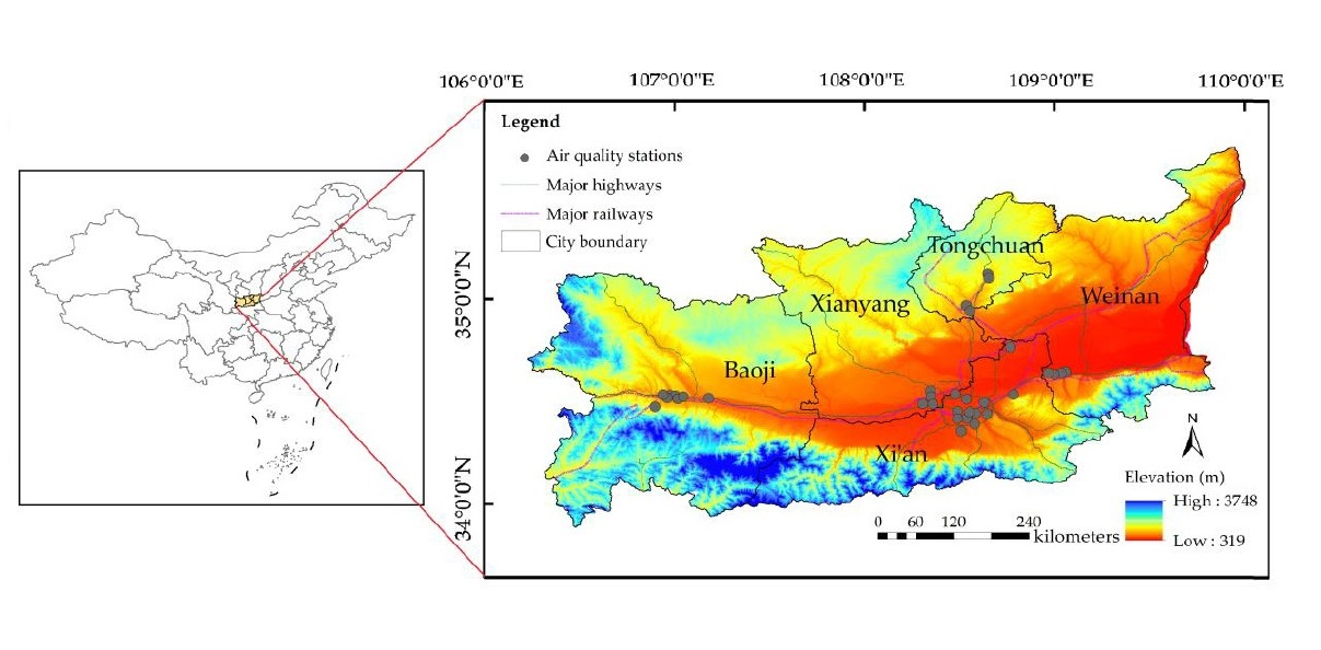
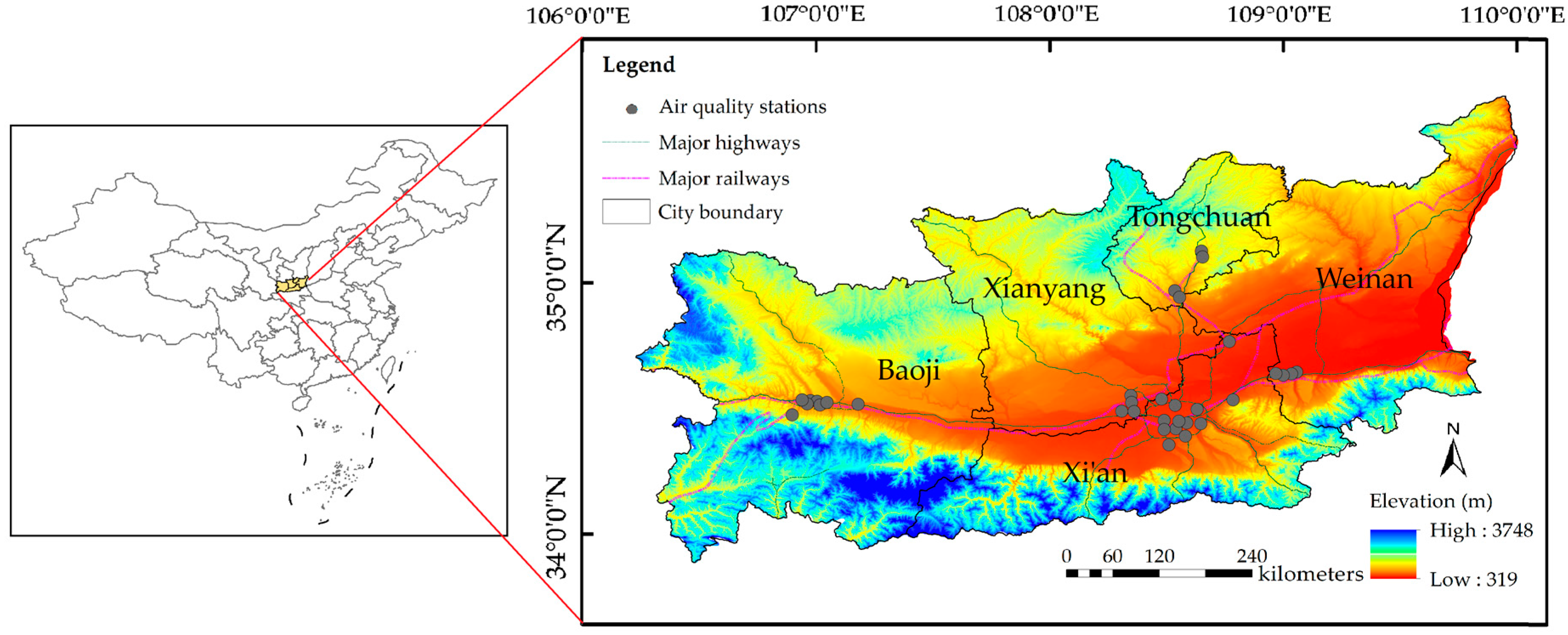
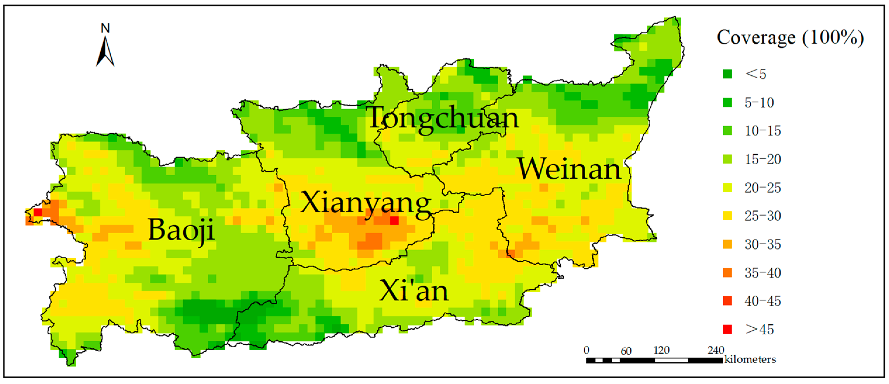
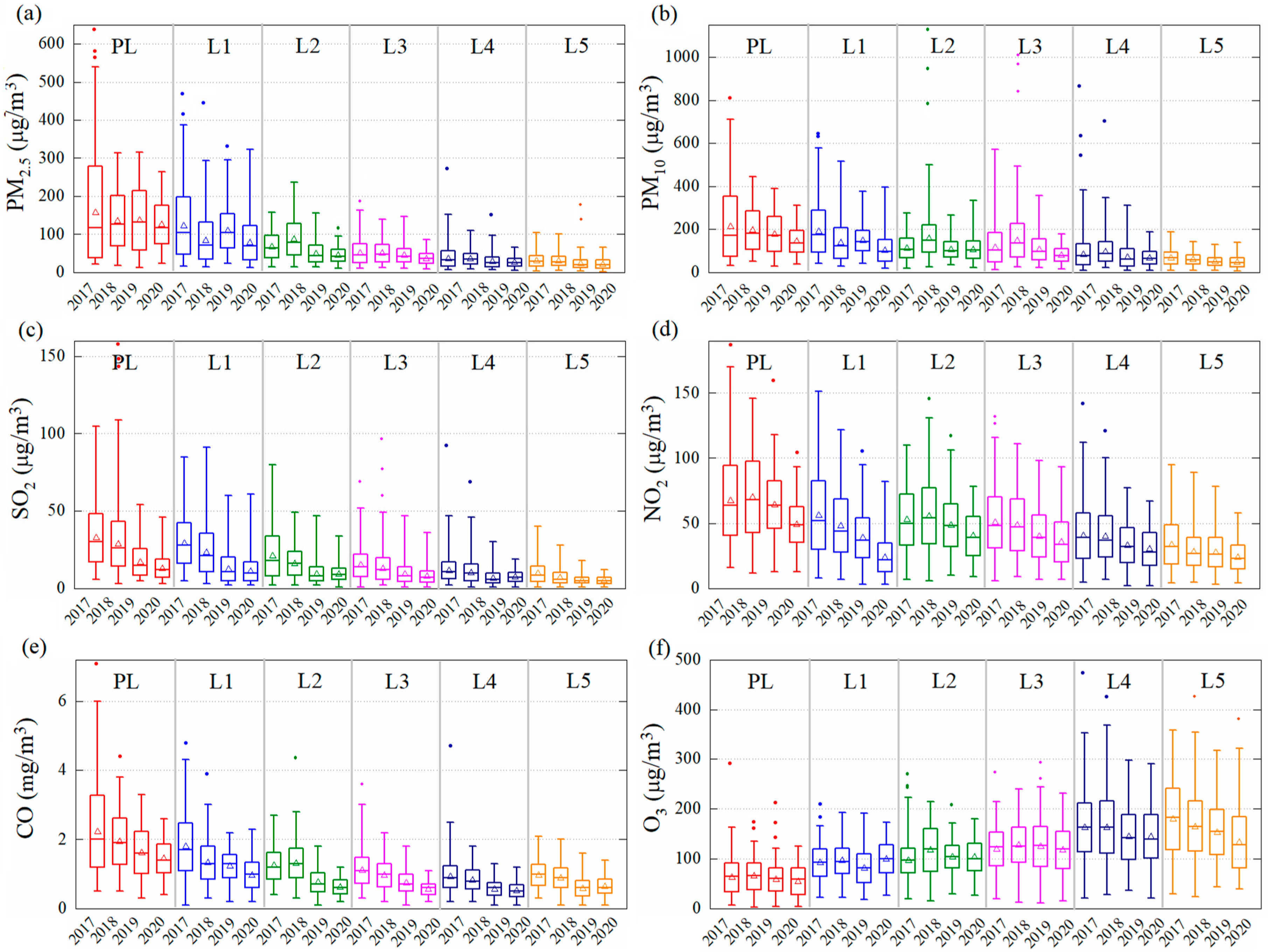
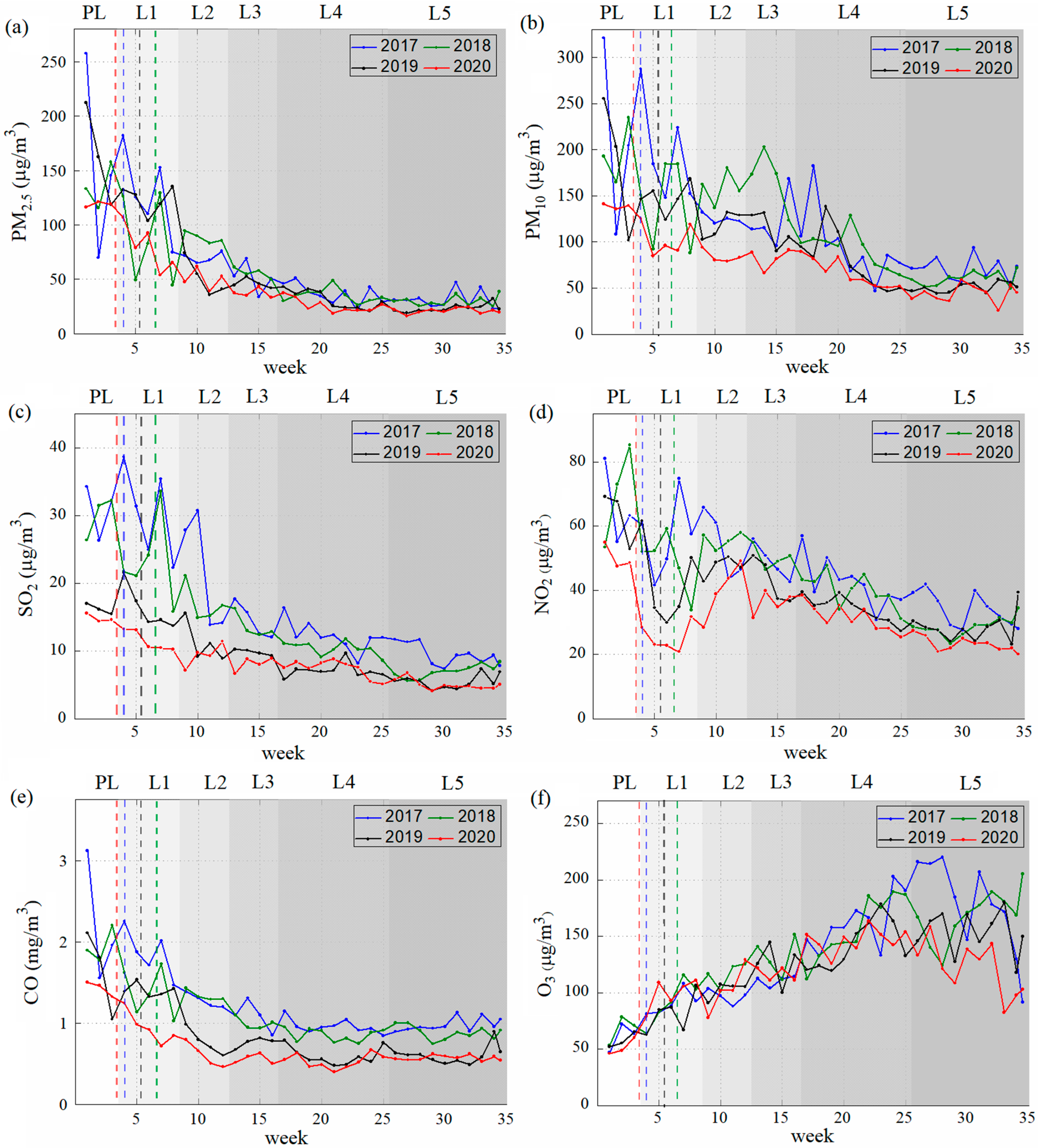
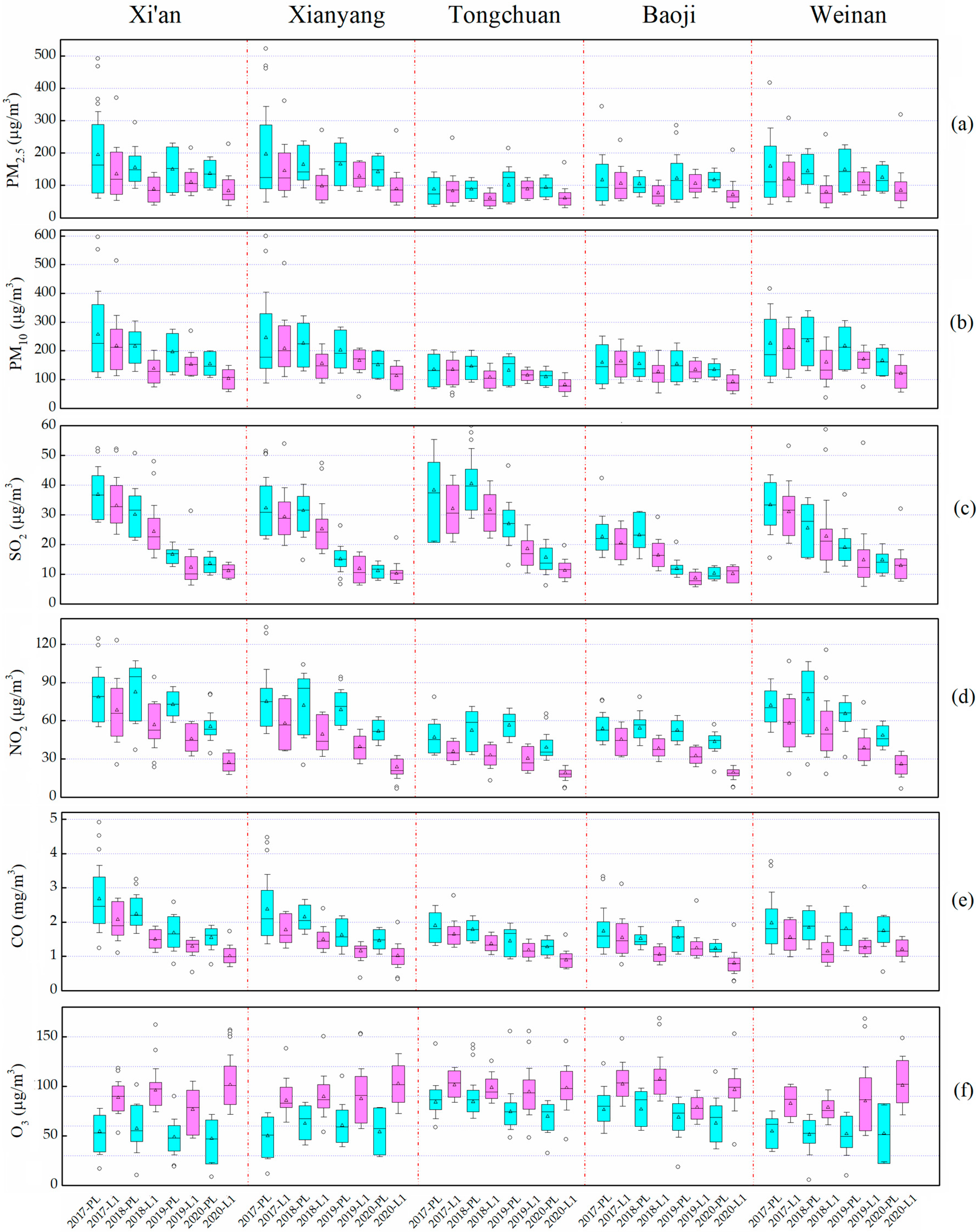
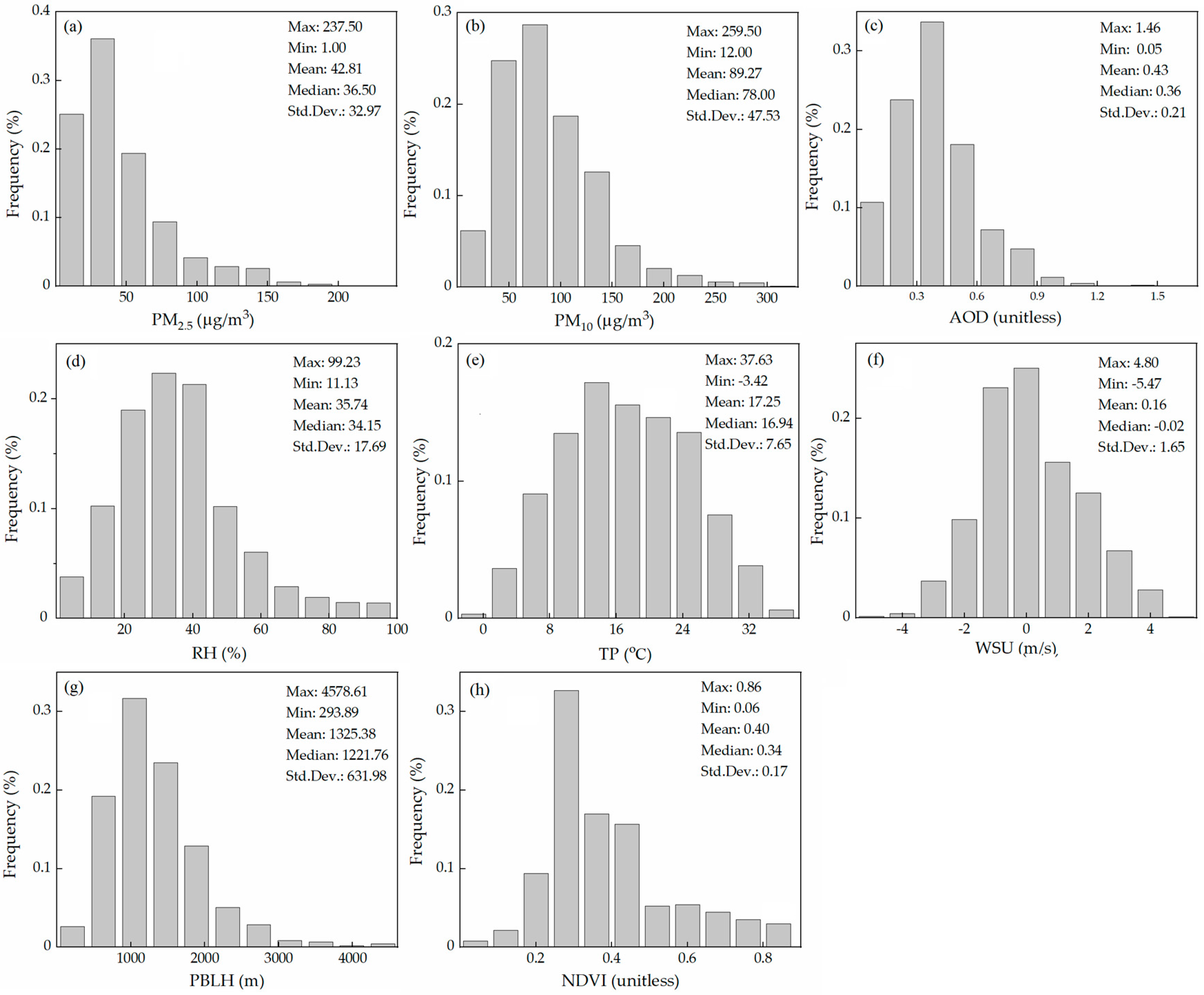
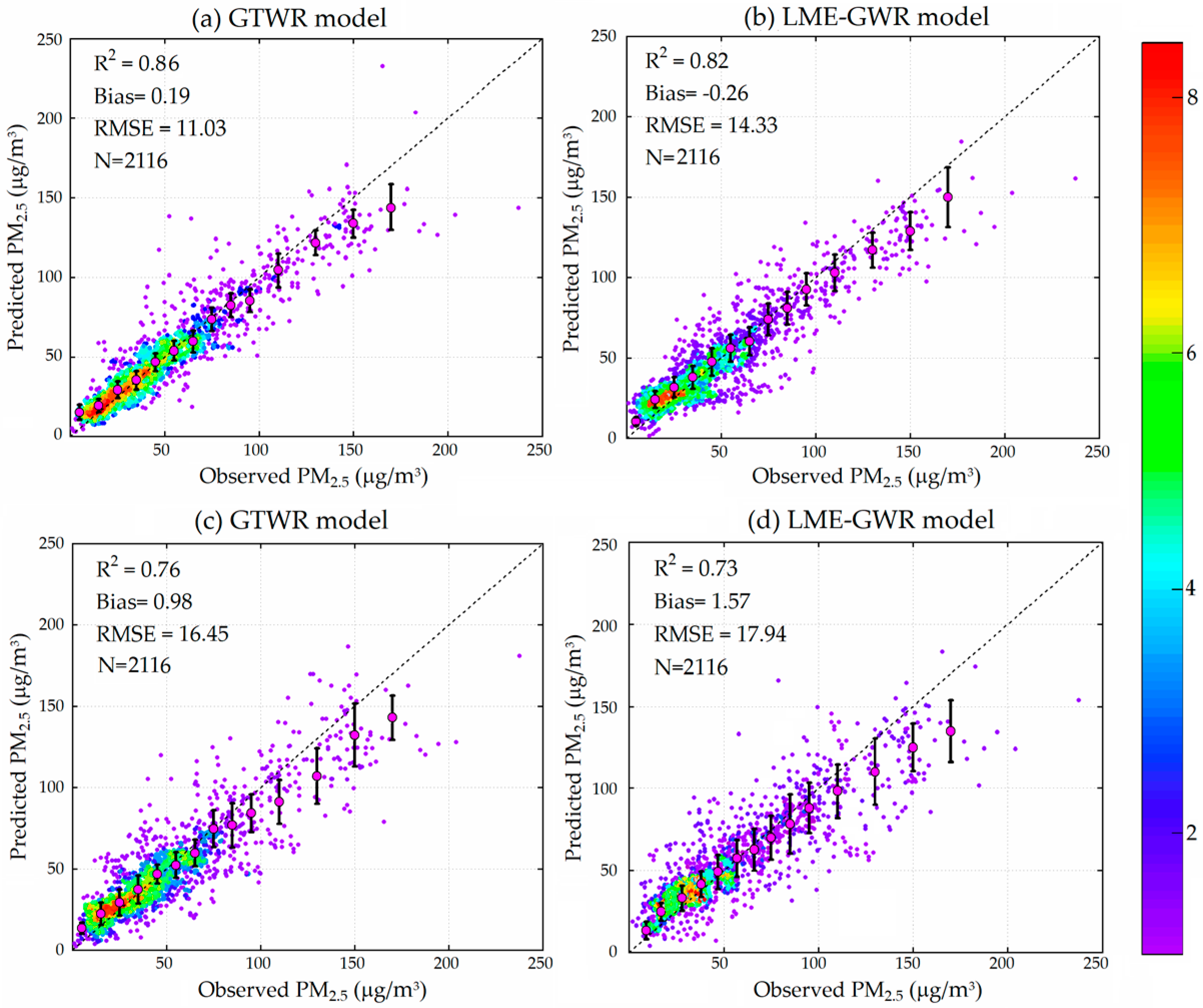
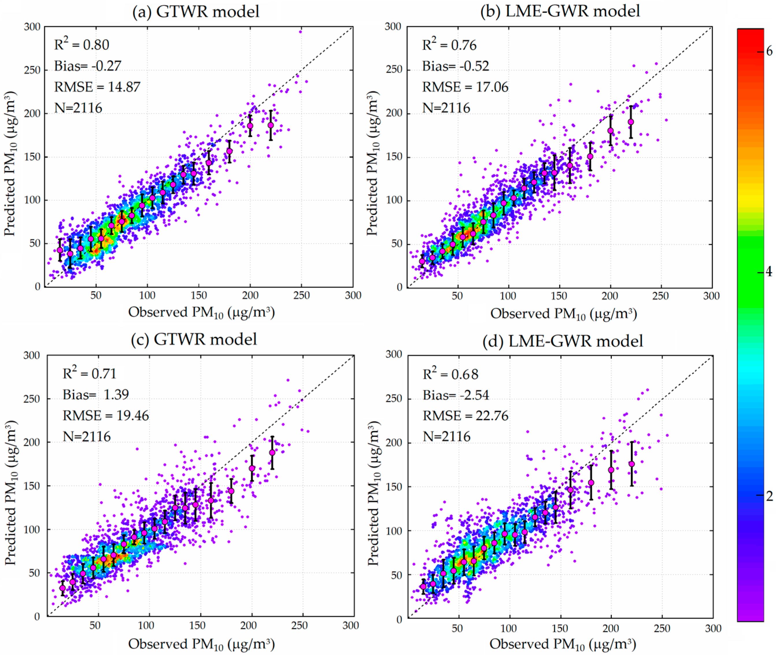
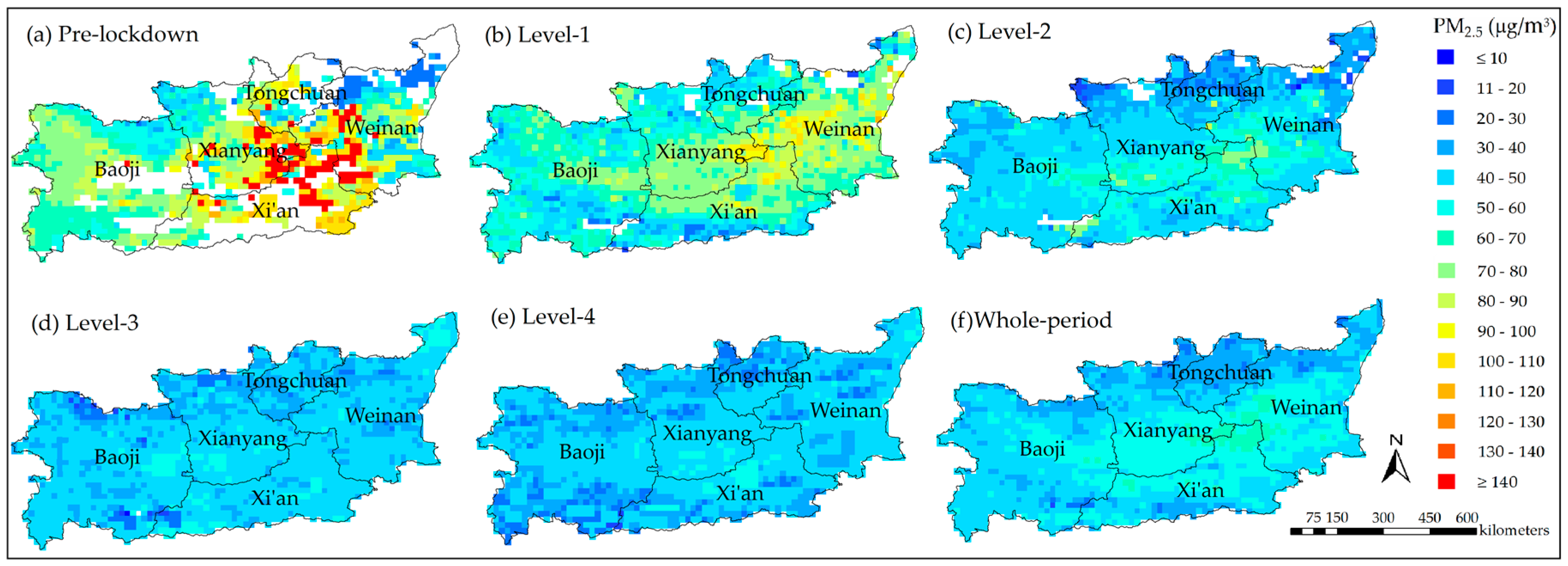
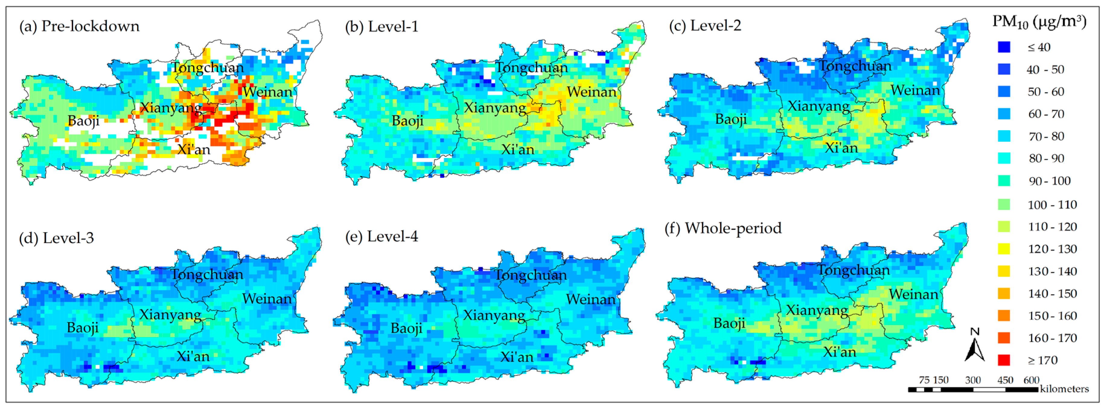
Table 1.
Correlation coefficients (R2) between each of the independent variables used for building the models.
Table 1.
Correlation coefficients (R2) between each of the independent variables used for building the models.
| AOD (Unitless) | TP (°C) | RH (%) | PBLH (m) | WSU (m/s) | NDVI (Unitless) | |
|---|---|---|---|---|---|---|
| AOD | 1.00 | |||||
| TP | 0.05 | 1.00 | ||||
| RH | 0.10 | −0.22 | 1.00 | |||
| PBLH | −0.14 | 0.27 | −0.37 | 1.00 | ||
| WSU | −0.11 | 0.15 | −0.06 | −0.06 | 1.00 | |
| NDVI | −0.08 | 0.35 | −0.19 | 0.02 | 0.01 | 1.00 |
© 2020 by the authors. Licensee MDPI, Basel, Switzerland. This article is an open access article distributed under the terms and conditions of the Creative Commons Attribution (CC BY) license (http://creativecommons.org/licenses/by/4.0/).
Share and Cite
MDPI and ACS Style
Zhang, K.; de Leeuw, G.; Yang, Z.; Chen, X.; Jiao, J. The Impacts of the COVID-19 Lockdown on Air Quality in the Guanzhong Basin, China. Remote Sens. 2020, 12, 3042. https://doi.org/10.3390/rs12183042
AMA Style
Zhang K, de Leeuw G, Yang Z, Chen X, Jiao J. The Impacts of the COVID-19 Lockdown on Air Quality in the Guanzhong Basin, China. Remote Sensing. 2020; 12(18):3042. https://doi.org/10.3390/rs12183042
Chicago/Turabian StyleZhang, Kainan, Gerrit de Leeuw, Zhiqiang Yang, Xingfeng Chen, and Jiashuang Jiao. 2020. "The Impacts of the COVID-19 Lockdown on Air Quality in the Guanzhong Basin, China" Remote Sensing 12, no. 18: 3042. https://doi.org/10.3390/rs12183042
Note that from the first issue of 2016, this journal uses article numbers instead of page numbers. See further details here.