Automatic Grapevine Trunk Detection on UAV-Based Point Cloud


1
Computer Graphics and Geomatics Group of Jaén, University of Jaén, 23071 Jaén, Spain
2
Engineering Department, School of Science and Technology, University of Trás-os-Montes e Alto Douro, 5000-801 Vila Real, Portugal
3
Centre for Robotics in Industry and Intelligent Systems (CRIIS), INESC Technology and Science (INESC-TEC), 4200-465 Porto, Portugal
*
Author to whom correspondence should be addressed.
Remote Sens. 2020, 12(18), 3043; https://doi.org/10.3390/rs12183043
Submission received: 26 August 2020
/
Revised: 14 September 2020
/
Accepted: 16 September 2020
/
Published: 17 September 2020
(This article belongs to the Special Issue UAS-Remote Sensing Methods for Mapping, Monitoring and Modeling Crops)
Abstract
:The optimisation of vineyards management requires efficient and automated methods able to identify individual plants. In the last few years, Unmanned Aerial Vehicles (UAVs) have become one of the main sources of remote sensing information for Precision Viticulture (PV) applications. In fact, high resolution UAV-based imagery offers a unique capability for modelling plant’s structure making possible the recognition of significant geometrical features in photogrammetric point clouds. Despite the proliferation of innovative technologies in viticulture, the identification of individual grapevines relies on image-based segmentation techniques. In that way, grapevine and non-grapevine features are separated and individual plants are estimated usually considering a fixed distance between them. In this study, an automatic method for grapevine trunk detection, using 3D point cloud data, is presented. The proposed method focuses on the recognition of key geometrical parameters to ensure the existence of every plant in the 3D model. The method was tested in different commercial vineyards and to push it to its limit a vineyard characterised by several missing plants along the vine rows, irregular distances between plants and occluded trunks by dense vegetation in some areas, was also used. The proposed method represents a disruption in relation to the state of the art, and is able to identify individual trunks, posts and missing plants based on the interpretation and analysis of a 3D point cloud. Moreover, a validation process was carried out allowing concluding that the method has a high performance, especially when it is applied to 3D point clouds generated in phases in which the leaves are not yet very dense (January to May). However, if correct flight parametrizations are set, the method remains effective throughout the entire vegetative cycle.
1. Introduction
The monitoring and management of agricultural crops, particularly with regard to nutrient level, water stress, diseases and pests, and phenological status, are vital for successful agricultural operations [1]. Traditionally, these activities are carried out through visual examinations of the crops, or by analysing plants and soil, which are time-consuming and invasive approaches [2]. Considering the fact that it is necessary to maximise yield and resources, while reducing environmental impacts, mainly by optimising the use of water and significantly reducing fertilisers and pesticides [3]. This can only be achieved by obtaining data that allow the intelligent and sustainable management of agricultural parcels [4]. It will then be possible, in a rational and economical way, to resort differentiated and localised actions with regard to the use of water and nutrients, and to control the soil and vegetation cover, as well as the plant’s phytosanitary status.
The technological advances in recent years, have enabled the miniaturisation of electronic components and a significantly reduction in prices, taking Precision Agriculture (PA) to another level. For example, the advent of Unmanned Aerial Vehicles (UAVs) capable of capturing aerial high resolution data using different kind of sensors (RGB, multi and hyperspectral, thermal and LiDAR), together with new photogrammetric processing methods, allow the computation of diverse outcomes such as orthophoto mosaics, vegetation indices and 3D point clouds [5]. UAVs are a popular tool in PA and the obtained aerial imagery is turned into information which can be used to optimise crop inputs through variable rate applications [6,7,8].
In a short period of time PA approaches and practices have become very popular and were introduced in all agricultural sectors [9]. The vine and wine sector is among those that have most benefited of precision farming techniques, applied to optimise vineyard performance [10]. Thus, the Precision Viticulture (PV) concept was introduced and can be defined as a particular field of PA, whose purpose is maximising grape yield and quality while minimising environmental impacts and risks [11]. Therefore, it is possible to avoid unnecessary treatments, which can be harmful and polluting, and reduce costs [12]. The ability of UAVs to obtain high spatiotemporal resolution and geocoded images from different sensors, make them a powerful tool for a better understanding of the spatial and multi-temporal heterogeneity of vineyard plots, allowing the estimation of parameters that directly affect its state. Thus, individual grapevine identification and location is of great importance to precisely assess the vineyard status estimating different parameters per individual plant [13]. However, there are many features in vineyards that make these scenarios very complex to develop automatic methods for trunk individual detection and location [14]. Therefore, segmentation methods that consist of processes of dividing input data into several disjoint areas that maintain the unique and homogeneous features from surrounding have to be employed.
Regarding vineyard vegetation detection, several methods were already proposed based on different approaches using the photogrammetric outcomes from UAV-based imagery by applying image processing techniques, machine learning methods and by filtering dense 3D point clouds and Digital Elevation Models (DEMs) [14,15,16,17,18]. Those methods are capable of distinguishing grapevine from non-grapevine vegetation and to extract different vineyard macro properties such as the number of vine rows, row spacing, width and height, potential missing plants and vineyard vigour maps.
The outcomes resulting from photogrammetric processing applied to UAV-based imagery can be used to estimate individual geometrical and biophysical grapevine parameters, providing a plant-specific application for PV [19]. In this scope some studies can be found in the literature. De Castro et al. [20] developed an Object-Based Image Analysis (OBIA) method applied to high-resolution vineyard Digital Surface Models (DSMs) to estimate grapevine vegetation. Then, the individual position of grapevines were marked, assuming a constant space between plants. This way, missing plants were also estimated and some geometrical parameters were estimated. In a different study, proposed by Matese and Di Genaro [21], missing plants detection was assessed in a semi-automatic procedure by filtering the DSM and by manually placing small polygons, representing individual plants and, then, analysing the number of pixels intercepted by each polygon by using a five-classes approach based on quantiles to verify the probability of a missing plant presence. A binary multivariate-logistic regression model was used by Primicerio et al. [22] for the individual detection of grapevines, including missing grapevines, in orthophoto mosaics. In the referred studies it is highlighted that the integration of other sensors data could allow the extraction of single plant vigour, health and water status. In this regard, Pádua et al. [13] performed an individual grapevine estimation for site-specific management in a multi-temporal context, helping winegrowers to fully explore the potential of the high-resolution data provided by UAVs and to combine data resultant from the different imagery sensors for a more precise decision support and a quick vineyard inspection. More recently, several studies have explored 3D point clouds resulting from UAV-based imagery photogrammetry processing to identify vineyards. Point cloud models consist of large datasets of points representing the surface of visible objects and can be derived from UAV-based imagery by photogrammetry and computer vision algorithms such as, for example, Structure from Motion (SfM). Alternatively, 3D point clouds can be directly provided by Light Detection and Ranging Systems (LiDAR). Comba et al. [23] proposed an unsupervised algorithm for vineyard detection and vine-rows features evaluation, based on 3D point-cloud maps processing. However, as final result, only the vineyards and local evaluation of vine rows orientation were retrieved. Comba et al. [24] applied a multivariate linear regression model to crop canopy descriptors derived from the 3D point cloud, to estimate vineyard’s Leaf Area Index (LAI). Marie Weiss and Frédéric Baret [17], applied a SfM algorithm to extract 3D dense point cloud over the vineyard and used the terrain altitude, extracted from the dense point cloud, to get the 2D distribution of height of the vineyard. Then, a threshold on the height was applied to separate the rows. Mesas-Carrascosa et al. [25] used 3D point clouds generated using photogrammetric techniques to RGB images acquired by UAV to derive vineyard canopy information. Additionally, to the geometry, each 3D point also stored the colour which was used to discriminate between vegetation and bare soil. Aboutalebi et al. [26] used UAV-based 3D information to monitor and assess vineyard plant’s condition. Different aspects of 3D point cloud were used to estimate height, volume, surface area, and projected surface area of plant’s canopy. Then biomass information was used to assess its relationship with in situ LAI. Other studies, such as that by Moreno et al. [27], used terrestrial LiDAR sensors to reconstructed vineyard crops. Although accurate, these methods are time-consuming and very expensive.
As it can be concluded, through the studies previously presented, there are many groups of researchers who are dedicated to the development of methods to extract useful information from vineyards. Although it is considered by everyone of fundamental importance the detection and location of individual plants, there are no methods capable of making it fully automatic. Indeed, the various methods found in the literature, are able to estimate the position of trunks, but using prior knowledge related to the number of plants per row and the distance between plants. Therefore, a fully automatic method able to detect and locate grapevine trunks is desirable and would have the potential to create base maps for most PV studies.
In this article, we present an innovative and fully automatic method able to detect and locate individual grapevine trunks, by exploring 3D point clouds derived from photogrammetric processing of UAV-based RGB imagery. The proposed method proved to be effective even when applied to complex vineyards plots. It is able to distinguish posts from trunks and to mark missing plants.
2. Materials and Methods
2.1. Study Area
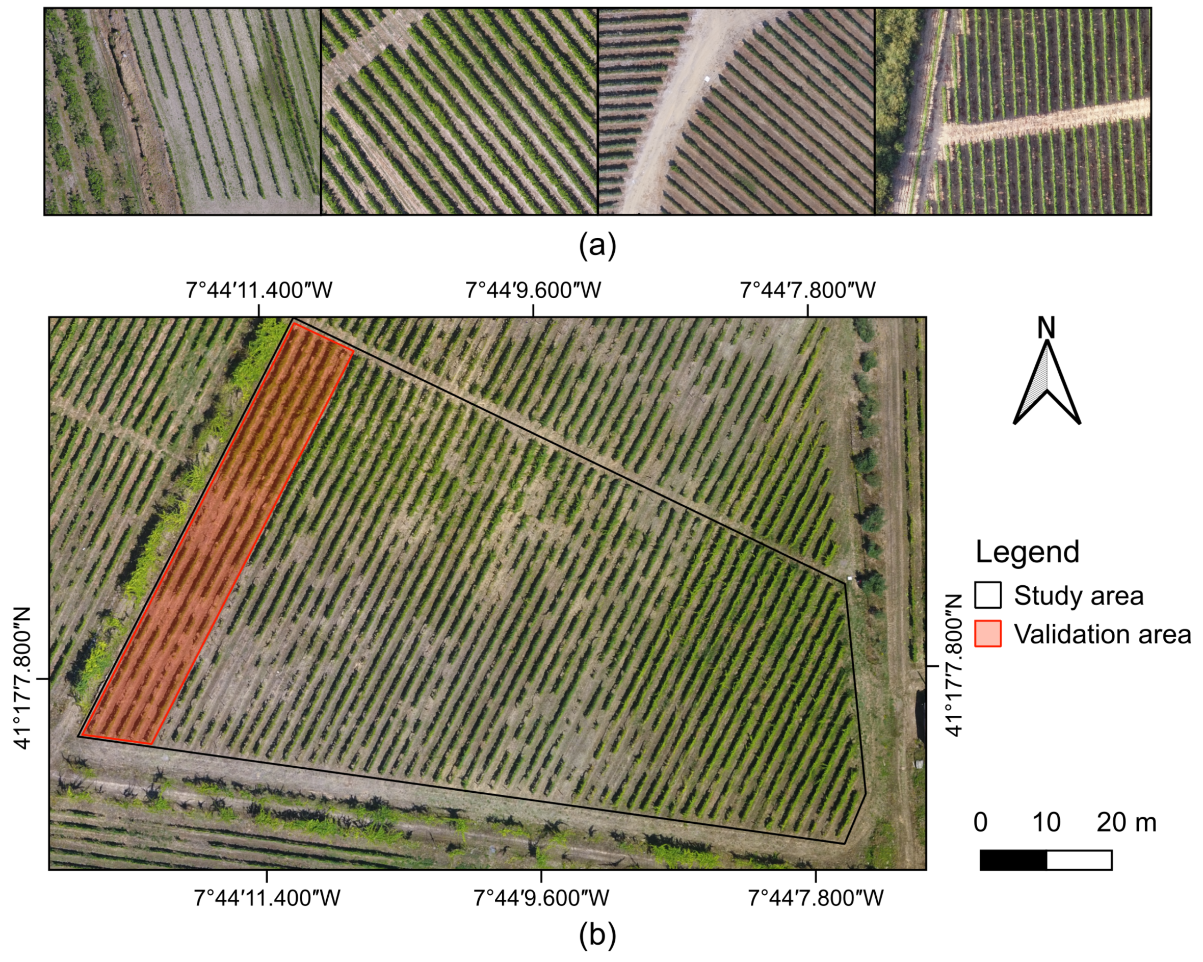
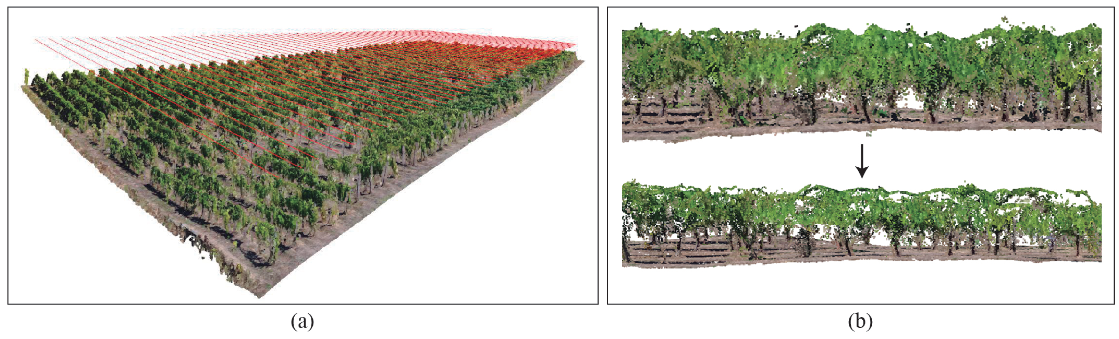
To develop the method proposed in this manuscript, several commercial vineyards (Figure 1a), in the northern region of Portugal, were selected to its application. Commercial vineyards usually present the great advantage of a proper management, where the best practices are applied to improve yield and quality. Therefore, these vineyards present well treated rows with a regular vegetative wall, facilitating the individual grapevine detection. Then, in the scope of this study, a complex and challenging vineyard plot was analysed (Figure 1b, 411708.1 N, 74409.9 W, 472 m altitude). The main purpose of using this vineyard, located in the campus of the University of Trás-os-Montes e Alto Douro (UTAD), Vila Real, Portugal, in the Douro demarcated region, was to push the method’s application to its limit. The plot has an area of 3200 m and is composed of 55 rows, and a double guyot trained system is used. The selection of this vineyard is based on the different levels of vigour and missing plants along the vine rows, providing a diverse variety of cases that are hard to be found in commercial vineyards.
2.2. UAV-Based Data Acquisition
Aerial RGB imagery acquisition was performed using the multi-rotor UAV DJI Phantom 4 (DJI, Shenzhen, China). Its native camera was used for RGB imagery acquisition, FCC 3 model, a CMOS sensor with 12.4 MP resolution mounted in a 3-axis electronic gimbal.
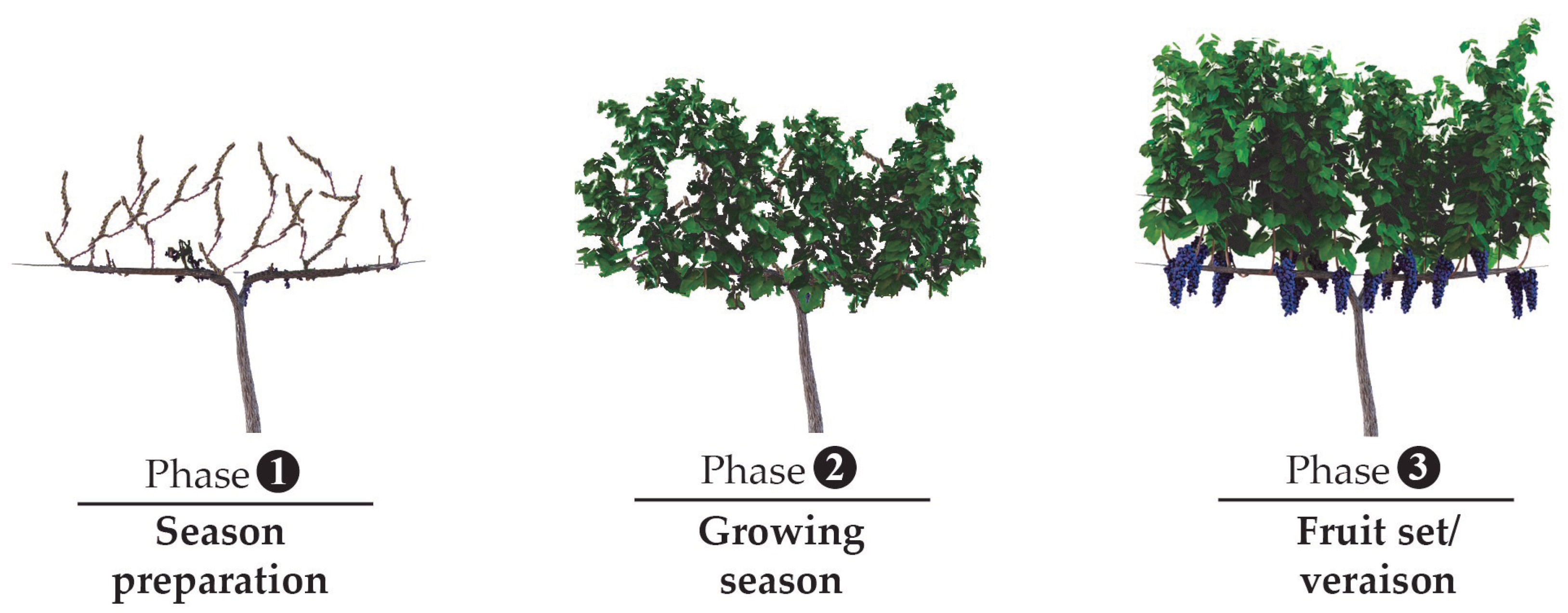
Different flights were conducted over distinct areas using a single-grid configuration and a flight height varying between 30 m (June and July flight campaigns) and 50 m (flights from January to May), from the UAV take-off position and with an imagery frontal overlap of 90% and 80% side overlap. The missions were planned and executed using DroneDeploy (California, CA, USA) in an Android smartphone. Regarding the most complex test site (Figure 1b), the flight was performed on 30 July 2019 and a total of 228 images were acquired. The whole flight campaign was carried in 13 min, five minutes for UAV assembly/disassembly operations and mission uploading, while the duration of the flight was eight minutes. The camera can be facing down, i.e., in the nadir direction, in all the flights conducted during the season preparation period. In the remaining flights, conducted in the growing and/or harvesting preparation period, the camera was used with an inclination angle of 65, relative to the nadir direction. This choice was done due to the absence or presence of leaves, capable of obstructing trunk detection (respectively, Phase 1 and Phases 2 and 3, of Figure 2).
2.3. Proposed Method
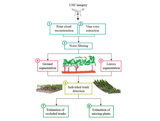
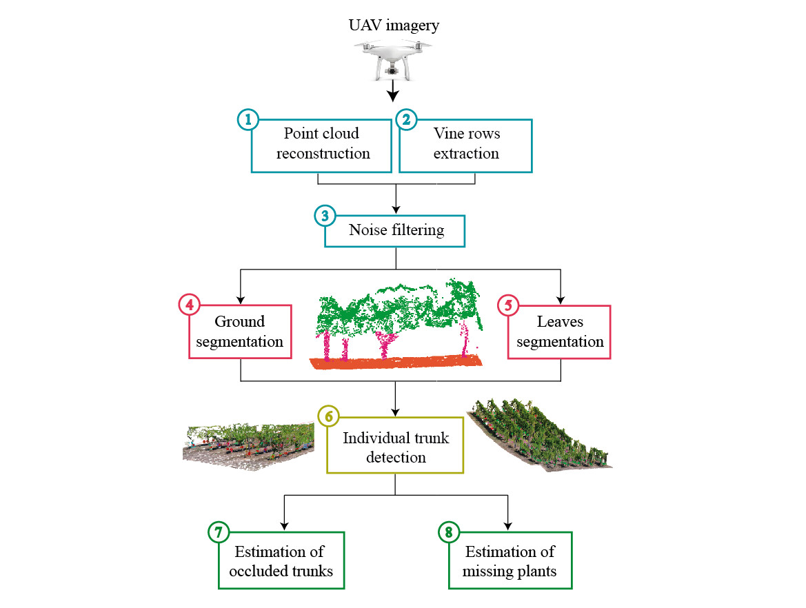
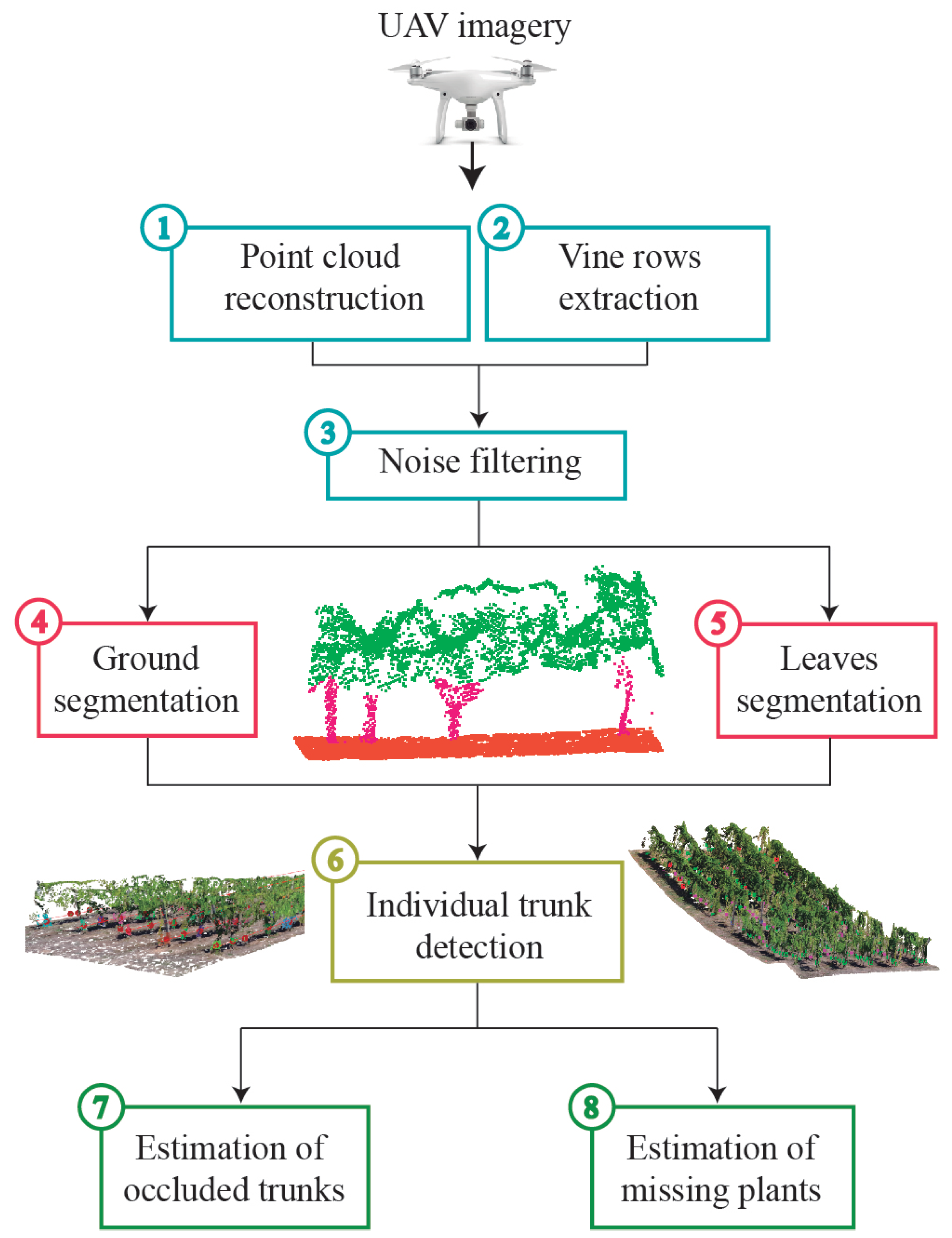
The main steps of the automatic grapevine trunk detection method based on a geometric segmentation on point cloud data are presented in Figure 3.
Firstly, the RGB aerial imagery are used to generate a 3D dense point cloud which was geometrically corrected using ground control points (GCPs). Then, a noise reduction is applied to remove many points which usually are close to the plant body. This step is important to achieve a more accurate trunk detection on areas with dense vegetation. Secondly, the location of vine rows is obtained in the form of lines using the method proposed in Pádua et al. [14]. In this way, the search area is confined to the vine rows only, optimising the whole process. Consequently, 3D points close to these lines were selected from the rest of the point cloud. Thirdly, a geometric segmentation is carried out in order to remove 3D points representing the ground and leaves. Thus, points belonging to trunks are isolated and spatial clustering can be performed. Finally, the 3D position for each grapevine is determined and, therefore, the number of existing and missing plants is calculated. The method was developed and implemented in C++ using the Point Cloud Library (PCL) [28].
2.3.1. SFM Reconstruction and Noise Removal
SfM techniques [29] are widely used for 3D reconstruction of multiple scenarios of the real-world [30]. These image-based methods are able to identify and match key points between overlapping images. In contrast to LiDAR-based solutions [27], the application of SfM enables collecting the fit-for-purpose data to model the geometry from some viewpoints. In general, plant modelling poses some challenges due to irregular surfaces, occlusion and varying illumination. In this regard, some considerations should be taken into account to process data correctly. For this study, 3D dense point clouds were generated over vineyard plots, by considering the following processing options: (1) a high overlapping rate (≥80%), (2) a valid key point must be visible in at least three images and (3) the image scale is set to 1/2 in order to increase recognisable key points per image. The photogrammetric processing of the acquired RGB imagery was performed using Pix4Dmapper Pro (Pix4D SA, Lausanne, Switzerland). A 3D dense point cloud was generated using the multi-scale half-image size, a high point density and a minimum of three matches per image. It was exported in polygon file format (PLY). Moreover, raster products were also computed after 3D point cloud interpolation using Inverse Distance Weighting (IDW).
Noisy points that inevitably surround the vegetation areas have to be removed in order to make an accurate geometric segmentation on the 3D model. The point cloud is filtered applying a noise filter which is provided by PCL, this method is based on the computation of distance between neighbours [31]. For each 3D point, the mean distance from it to all its neighbours is computed. Thus, all points whose mean distances are outside an interval defined by the global distances mean and standard deviation are considered to be outliers. The neighbour search was developed by considering a specific radius which is related to the point cloud density. The several tests performed allowed to conclude that 0.05 m should be used to increase method’s and results’ quality. By applying this noise filter to the 3D point cloud, most of erroneous 3D points in the lower parts of the grapevines were removed, allowing a better recognition of the trunks.
2.3.2. Vine Rows Extraction
In order to reduce the research area, the method proposed by Pádua et al. [14] is first applied. In this way, the vector lines representing individual axis of vine rows are identified. In short, the identification of the lines is based on the use of a crop surface model—computed from the subtraction of the DEM to the Digital Surface Model (DSM)—in combination with the green percentage index (G%) [32], computed using the red, green and blue bands of the orthophoto mosaic. Then, grapevine vegetation is estimated from the threshold and concatenation of both raster products— the Canopy Surface Model (CSM), according to a height range and the G%, by using the Otsu’s method [33]. After this procedure, a binary image is generated with a set of clusters of pixels mostly representing the grapevine vegetation. In this way, the vine rows and its central lines are estimated, considering the orientation of the most representative clusters.
Thus, the estimated vine rows axis (central lines) are used as a virtual guide to create a buffer allowing identifying points which compose the plant geometry and the surrounding soil (see Figure 4a). Since the vegetative wall width of grapevine plants usually varies between 30 and 50 cm, it was decided to create a 60 cm buffer to selected 3D points to be analysed. As it is shown in Figure 4b, the green points represent the selected points considering 30 cm width to each side the vine row.
2.3.3. Ground and Leaves Segmentation
The vine rows extraction method enables removing 3D points, which were outside of 3D buffers. However, in addition to points, which potentially may define the trunk’s geometry, there are other 3D points in the vine row space to be discarded. In order to isolate trunk points, it is necessary to remove those 3D points representing leaves, which usually appear in the upper section of the point cloud and ground points, which are located in the lower part of the 3D model. For this purpose, only geometric and spatial features as well as the point colour were considered, and the following three steps strategy was applied: (1) spatial subdivision of the vine row buffers, based on height thresholds, (2) ground removal (3) leaves removal. This process is fully automatic and no human intervention is required. In effect, the method has the ability to be applied even in vineyard plots with irregular slope, distinct density of plant foliage and voids (missing plants) along the vine row.
However, and before the application of the this procedure, 3D buffers need to be divided in different segments (Figure 5). This subdivision is determined based on the buffer’s length and the terrain’s slope. In this task, it is crucial to apply height thresholds, mainly important if the terrain slope varies. In flat terrains this step could be avoided, still to keep the method as general as possible, it was decided to include this step. If the terrain’s slope is irregular, a higher number of segments will be required to allow a better fit. By default, the segment length is set to 1 m since it proved to fit most scenarios.
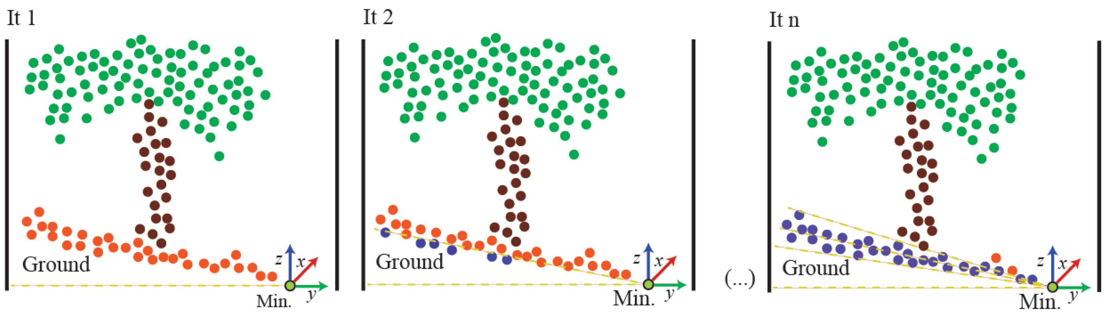
The leaves and ground removal operation is carried out by considering the vine row buffers segmentation. In fact, the following geometric operations were developed for each segment. Firstly, 3D points with the highest and lowest heights are detected. Then, the terrain’s slope is fitted by changing the orientation of a cutting plane for n iterations. Thus, ground points which are under this plane were automatically discarded. Figure 6 shows the main iterations of this step.
Initially, this 3D plane is fixed by the point with the minimum height and the up vector (v = 0,0,1), whose direction is perpendicular to the horizontal plane. Then, for each iteration, the plane is rotated 5 around the x-axis. This geometric transformation was performed by applying the rotation matrix showed in Equation (1). The stopping criterion was determined by several 3D points, selected in each iteration, i.e., those which were under the cutting plane influence. The plan inclination angle is set to the value allowing a proper fit of 3D plane to the terrain slope. Finally, to determine the location of points relative to the cutting plane, the point-normal equation for the cutting plane was applied. If the result is lower than zero, the point is under the plane (Equation (2)), so it is classified as ground and automatically removed in the point cloud.
where A, B and C represent the coefficients of the normal vector, (x, y, z) represent the coordinates of the point on the plane and (, , ) represent the coordinates of 3D points.
Regarding the leaves removal, the same inclination angle used for the ground cutting plane was applied. To fix the position of this upper plane, an offset value was calculated considering points with the maximum and minimum height for each segment. This procedure is illustrated in Figure 7.
After ground and leaves points removal, the next step consists in the identification of individual trunks. This is done based on the application of a spatial segmentation especially developed for that purpose. In this regard, the trunk is considered to be a 3D geometric shape, and a clustering method sharing the following features was developed: (1) the Euclidean distance between the 3D points must be lower than 50 cm (this value is estimated considering the typical distance between grapevines, which is never of this order); and (2) the minimum number of points for clustering is set to five. According to these constraints, a correct limitation of the growing region was determined for each cluster. Therefore, n groups of points were segmented for each vine row.
The value h represents the vertical height of plants in the segment, while the value f represents the offset obtained by applying Equation (3). According to this setting, the top plane was adapted by the geometric features for each segment. In this case, upper points to the cutting planes, which were considered vegetation, were removed in the point cloud. However, some outlying points could not be correctly filtered by the cutting plane. For this reason, another filter was applied based on the point colour. A threshold for the green channel was fixed in order to remove vegetation points characterised by the green channel higher than 120 as well as red and blue channel lower than 80. This combination was considered adequate and derived from the many tests performed. Lower values would cause the removal of points belonging to the trunks.
2.3.4. Trunk Detection
After ground and leaves points removal, the next step consists in the identification of individual trunks. This is done based on the application of a spatial segmentation developed for that purpose. In this regard, the trunk is considered to be a 3D geometric shape, and a clustering method sharing the following features was developed: (1) the Euclidean distance between the 3D points must be lower than 50 cm (this value is estimated considering the typical distance between grapevines, which is never of this order); and (2) the minimum number of points for clustering is set to five. According to these constraints, a correct limitation of the growing region was determined for each cluster. Therefore, k groups of points were segmented for each vine row.
Regarding the results of spatial clustering, two optimisations are considered to improve the final results. The first optimisation focuses on solving errors related to the spatial segmentation. In areas characterised by dense vegetation, where the trunk was partially occluded by leaves, the trunk’s 3D reconstruction is, in general, generated with a lower detail. In these cases, the trunk is potentially composed by a few real points and many noisy points. Consequently, an inaccurate segmentation is achieved, which causes false positives in those regions. This issue is overtaken by testing the angle () between two vectors: (1) the direction vector of the vine row axis; (2) the direction formed by two consecutive centroids of clusters. A maximum deviation of 20 is allowed. This value proved to be adequate to remove clusters which are not correctly segmented. As illustrated in Figure 8, green points are valid centroids and red points are those centroids which are discarded. The blue arrows depict the correct patch formed by all plants of the row. This test is performed along the vine row in the same direction on the x-axis.
The second optimisation consists on the automatic recognition of posts, which are considered to be trunks, since geometrically both are very similar. For this purpose, key geometric features were considered to detect posts for each vine row. In Figure 9a, trunks and posts are marked by a green and yellow rectangle, respectively. The main difference is the number of vegetation points around them. As shown in Figure 9b, a neighbour search is developed for each centroid, limited by a radius (r = 80 cm). This value is the most adequate considering the mean size of grapevines in the dataset. To check points which were into this spherical-searching region, Equation (4) is applied. Then, the point colour is also considered in order to detect vegetation points. Vegetation points are characterised by a threshold for the R, G and B channels so, if some of them are located inside the search area, the cluster is considered to be trunk. Likewise, if no vegetation points are found, the cluster is classified as a post.
where for each cluster, x, y and z represent the coordinates of a 3D point and r the radius of the search region.
2.3.5. Estimation of Missing Plants and Occluded Trunks
Depending on the epoch of the year in which data are acquired, vegetation may occlude trunks (Figure 2). The proposed method is also prepared to deal with such scenarios, being able to estimate the position of no visible trunks and missing plants. In general, and mostly in recent commercial vineyards, each vine row is formed by plants which are equidistant from each other. However, the presented method estimates the space between plants automatically, which makes its use universal and fully automatic. For testing this feature, the method was applied on a complex vineyard plot presented in Figure 1. Therefore, the method can be used in any vineyard even in those which present challenging features such as the irregular distance between plants, replanted grapevines with different trunk diameter and some plants not visible from aerial images due to a dense foliage (Figure 10).
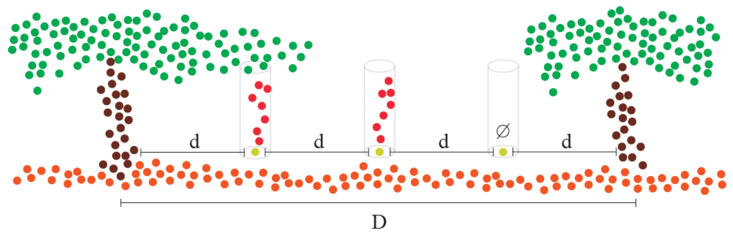
The estimation of missing plants and occluded trunks is useful in order to optimise the results of plant recognition as well as to know the number of voids along the vine rows, which could be occupied by new plants. For this purpose, the resulting data from the individual grapevine detection were used in order to identify areas where no plants were found. Firstly, the distances between consecutive grapevines are calculated and sorted from the lowest to the highest, considering all plants detected in a given vine row.
Then, all distances less than 50 cm are discarded and the top 10% values of the sorted list are used to calculate the average distance (d). This value was calculated for each vine row and is also used to highlight areas that can potentially contain missing plants or occluded grapevines. If the distance between two consecutive plants (D) is higher than d, and the rate is higher than one, the integer part of the quotient represents the number of plants that should be detected in the area. Then, missing plants and/or occluded trunks are marked using the average distance (d) as reference. Figure 11 illustrates the representation of two detected grapevines and the area between them where there are missing plants and occluded trunks. The last step consists in determining if the marked point represents a missing plant or an occluded trunk. To this end, a point inclusion test in a three-dimensional cylinder (height of 1 m and a radius of 20 cm) is implemented, considering the same constrains which were used for the trunk detection.
2.4. Validation Process
To analyse the robustness and effectiveness of the proposed method in all its features, five vine rows of the complex study area (polygon highlighted in Figure 1) were used. A field campaign was performed in order to map the real state of vine rows and to determine the location of missing plants. This way, for each vine row, the results provided by the application of the proposed method were compared with ground-truth data allowing computing the overall accuracy of the whole validation area and of each estimation.
Grapevine estimation evaluation was conducted based on the number of correct (true positive—TP) and incorrect (false positive—FP) grapevine estimations and also considering the correct/incorrect estimation of missing plants along the vine rows as, respectively, true negatives (TN) and false negatives (FN). From theses data precision, recall, F1score and the overall accuracy were computed for each vine row and for the whole validation area.
3. Results
3.1. Point Cloud Reconstruction and Processing
The proposed method works perfectly when it is applied to well-maintained commercial vineyards plots, using aerial data acquired as described in Section 2.2. In those cases, the method is able to detect all existing trunks. However, the method was pushed to its limit, being applied to a complex area, arising from the existence of distinct vegetation density/vigour areas, several voids caused by missing plants, and new plants that were replaced defective or dead plants.
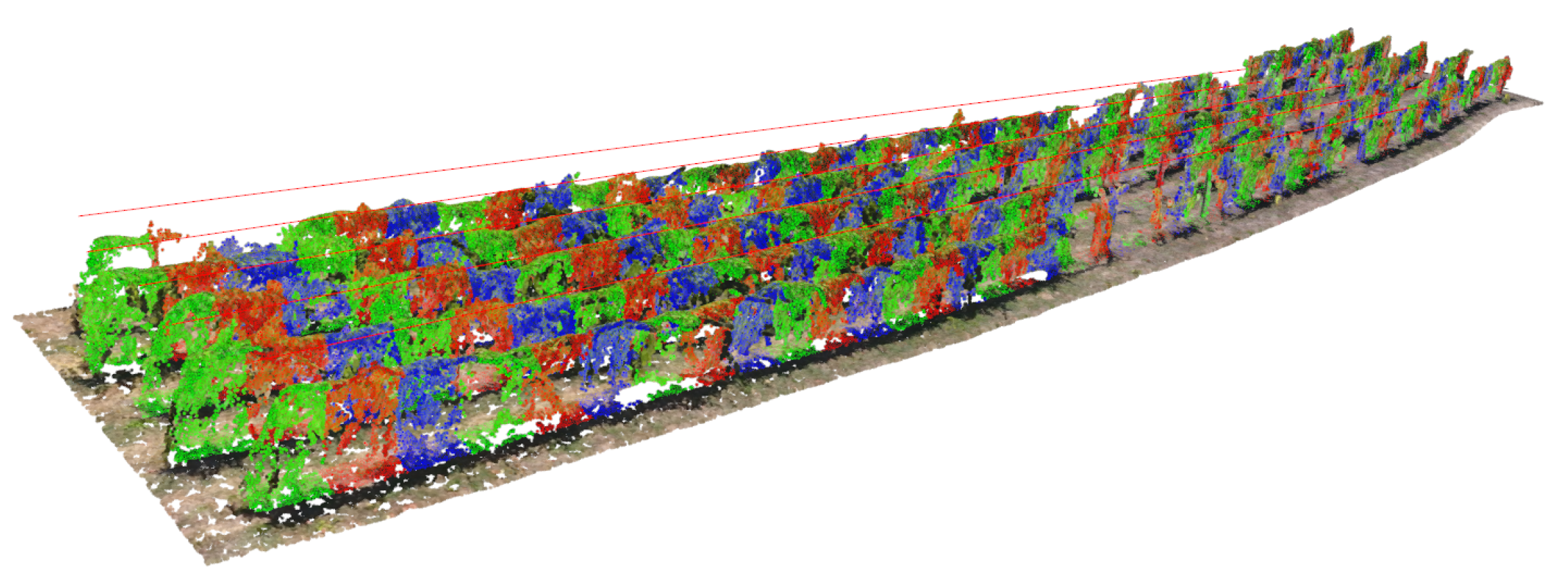
As results, a 3D point cloud formed by 26,656,371 points was generated and the time for point cloud densification was 01 h:29 m:23 s. Figure 12 shows the generated point cloud and the virtual lines that represent the vine rows axis. Most of plants could be fully modelled, but there are some grapevines whose trunks were partially occluded by leaves. Moreover, noisy points were produced around the trunks, between the leaves of plants and the ground. These 3D points negatively affect the recognition of trunk’s shape. To address this problem, a noise filter was applied and most of noising points could be removed. This process was applied using a kernel size of 0.05 m. In summary, 10.448.046 points were discarded in the generated dense point cloud.
3.2. Individual Grapevine Detection
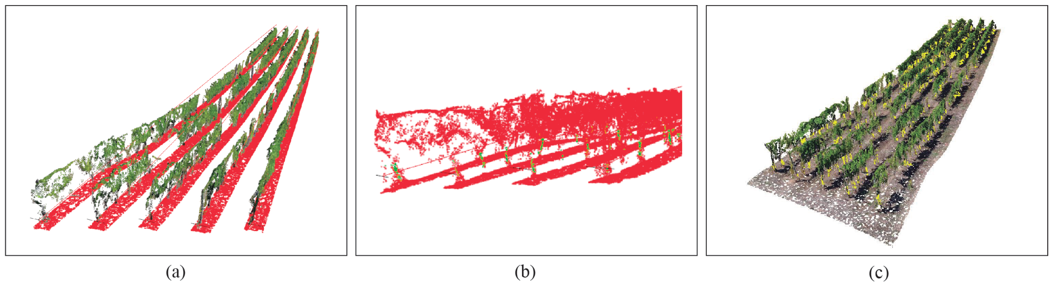
Once the point cloud is generated and the noisy points filtered out, the 3D model is segmented in order to discard ground and leaves points. Figure 13 shows the results of this step, when the method is applied to the vine rows of the validation area. Consequently, red points (classified as ground and leaves, Figure 13b) are discarded and just trunk points, which will be used as input data for the spatial clustering, remain.
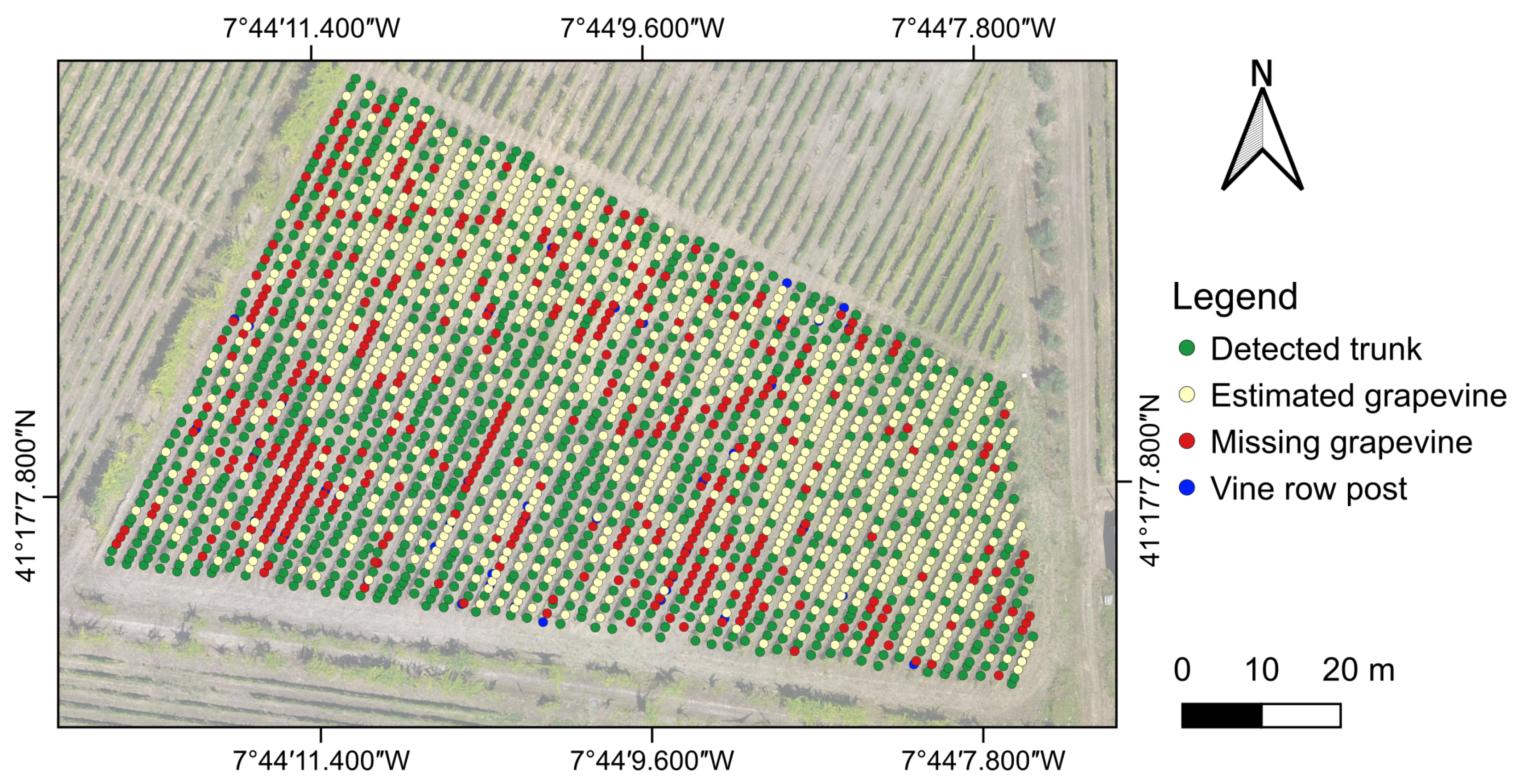
The method was applied to the whole plot and the location of detected and missing plants was analysed in the QGIS software. This output is presented in Figure 14, with the orthophoto mosaic in the background. A total of 1916 grapevines were estimated and 402 plants were classified as being missing.
Regarding the efficiency of the method, the time required for the automatic recognition of each individual grapevine in the whole plantation was 38 s using a PC with CPU (Intel Xeon(R) W-2145) and RAM (64 GB). The low time required for computing the methods makes possible the use of portable devices for on-site processing.
3.3. Grapevine Estimation Accuracy
The results of the grapevine estimation from the application of the proposed method to the five validation vine rows are presented in Table 1.
Regarding the total number of grapevines presented in the evaluated vine rows (ranging between 39 to 46), an overestimation of five plants is observed. Under detection of grapevines is verified in two rows, differing in three and two grapevines, respectively. The opposite is observed in the other three vine rows, with ten plants being overestimated (respectively, three, six and one). According to the number of missing grapevines (69, in total, ranging between 7 to 18 per row, average of 14 missing plants) the results obtained by the method show an overestimation of six missing grapevines in two vine rows (three in each) and one vine row is in agreement with the ground-truth data. As for the other vine rows the under estimation of missing plants diverges from three to eight plants (64 missing plants in total, with an average of 13 missing plants per row, 93% overall accuracy). As for the total number of possible grapevines in a given vine row (sum of the grapevines and missing grapevines), a mean of 57 plants were estimated, the same number when observing the ground-truth data, being the total also 285 plants, obtaining three rows with the same number of plants, two rows with one plant less, and one row with two plants more. For this specific parameter, the overall accuracy ranges between 97% (underestimation) and 100% considering all vine rows. According to the capability of the proposed method in the automatic detection of grapevines, 157 grapevines (71%) were directly detected from the grapevine trunk, and by the analysis of the point cloud density 64 grapevines were estimated. Moreover, several posts were also detected along the vine rows and therefore, were automatically discarded.
To further validate the spatial accuracy of the methods outputs, each detection was analysed to assess if the estimations were correctly located. By using the ground-truth data, false negatives and false positives results—grapevines classified as being missing and the inverse, missing plants classified as being grapevines—are evaluated. Table 2 presents these results. In total, from the 221 estimated plants 197 plants were correctly detected and classified (89%), as for missing plants, 41 (64%) were correctly classified, the overall accuracy considering all data is approximately 84%.
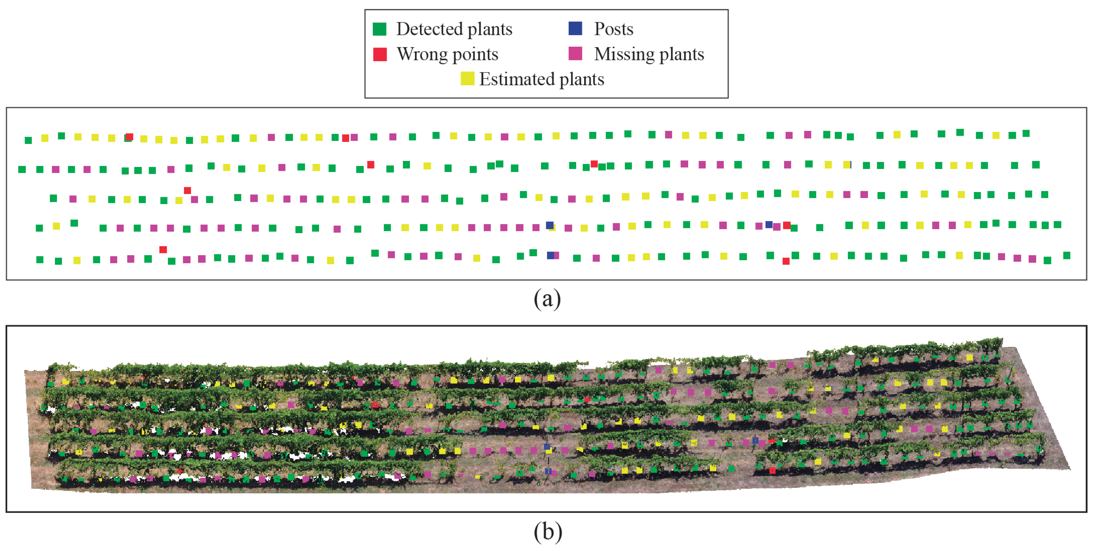
Figure 15 shows the 3D location of each plant on the test area. Green points represent the centroids of plants that are directly detected in the 3D model. The centroids’ position were then checked against its corresponding vine row in order to identify centroids wrongly classified as trunk (red points). These wrong classifications are caused due to points of vegetation, which are around the trunk and could not be totally removed by the noise filter. Then, posts were distinguished from the grapevine trunks (blue points). Finally, missing plants (pink points) and occluded trunks (yellow points) were estimated. In terms of quantitative data, in the validation area, the proposed method was able to detect 221 plants and 64 missing plants.
4. Discussion
4.1. Point Cloud Reconstruction and Processing
The generation of point clouds for remote sensing applications was enhanced by the proliferation of innovative UAV-based technologies such as high-resolution cameras and LiDAR systems. By applying photogrammetric techniques, point clouds can be obtained using multiple overlapping images. Other option is the use of LiDAR scanners which provide dense point clouds of natural environments but these are more expensive than digital cameras [34]. LiDAR data discriminate better plant’s canopy since it penetrates vegetation [35,36], and, therefore, potentially making the identification of the grapevine trunks easier. Moreover, photogrammetric techniques tend to estimate erroneous points in the cases where some points from the ground are estimated along a post. One of the advantages of the proposed method is that it remains operational even when using point cloud data from other type of sensors, reinforcing that when LiDAR sensors for UAVs become more affordable the method can still be employed. The proposed method is not dependent on any technology, although to get proper results is required enough geometric quality of the 3D model to ensure a partial reconstruction of the trunks at least. In this sense, to avoid noisy points around the trunk and vegetation, the presented solution integrates a noise filter. Hence, the proposed method can be applied using any point cloud data with accurate results.
4.2. Individual Grapevine Detection
There are several methods for the automatic detection and parameters extraction on 3D models using crop height models [37], combining terrestrial laser scanner and UAV photogrammetric point clouds [38], fusing RGB and multispectral point clouds to extract individual tree parameters [39], computing 3D vegetation indices in olive groves [40], and obtaining forest structural attributes [41]. However, given the complexity and the unique characteristics of vineyard plots, such methods are not suitable to be applied. Studies focusing on the use of photogrammetric point clouds, generated from UAV-based imagery, were dealing with vineyard detection [23] or detect and describe some of its general properties [17,25,42]. Studies for individual grapevine detection using UAV-based raster outcomes often rely on the coarse position of each vine assuming a mean distance of separation between grapevines along the vine row [13,20,21]. The proposed method addresses all these limitations, using point cloud data and geometrical characteristics, to automatically identify points belonging to grapevine’s trunk. Hence, individual plants can be detected and missing plants estimated.
The complex vineyard plot analysed in this study had been used in another study [13] with data acquired in 2018. The whole plot contained 2266 plants and was evaluated by the method with an accuracy of 98%. However, the aerial imagery was acquired in an early phase of the vegetative state [43] with a lower vegetation density, which can help in the detection of missing plants. Furthermore, a constant distance between individual plant was also used. The results presented in Section 2.4 present an overestimation of 2% (Table 1) according to the number of grapevines and an under-estimation of 8% considering the number of missing plants. This fact is related to the presence of vegetation from adjacent grapevines in areas with missing plants that could cover the void. The results are improved by selecting an early period (preferably belonging to phase 2—Figure 2) to conduct grapevine detection, with grapevines with a lower leaf cover, preventing the existence of vegetation in areas with no plants [21]. In Di Gennaro and Matese [44], 3D and 2.5D methods were compared for vineyard biomass and plant detection, but individual grapevine detection was not performed. In that study, as for missing plants, an overestimation was observed in the 3D-based method, false negatives were related to the existence of new plants while some false positives were due to different grapevine canopy thickness. Similar findings were detected in the miss-classifications observed in this study (Table 2). Moreover, proximal sensing approaches for grapevine trunk detection using ground vehicles were also tested by research groups, either using LiDAR [45,46] or depth cameras [47]. However, in contrast to UAVs, such approaches are more expensive—due to the equipment used—and time-consuming, since the vehicles need to go through all vine rows, where some obstacles can also be present in their way.
5. Conclusions
The innovative method presented in this study is proved to be effective for a rapid access of the vineyard status using UAV-based 3D point clouds, with automation levels that allow its applicability in different vineyards, not relying on predefined parameters as the distance among plants. The proposed method is able to detect occluded trunks with reliable accuracy rates and missing plants, where in the vineyard context represents the occurrence of voids along the vine rows. The major contribution of this work is that the approach is fully automatic, not requiring any a prior knowledge of the distance between plants or number of plants per row, as in existing approaches. Moreover, the computational complexity of the proposed technique does not require high-performance computing and is appropriate for use on mobile in-field computing devices.
The applicability of the proposed method can be extended to other types of purposes related to the estimation of biophysical parameters of grapevines, providing a more efficient understanding of data for vineyard management and the validation of the use of UAV-based point clouds. Indeed, its impact is increased in a multi-temporal context. In this way, the estimated canopy of each detected grapevine can be studied to measure its volume which can help in the decision-making process for canopy management operations and, consequently, yield optimisation. To improve data quality and to extend the method capabilities, an in-depth investigation of the flight parameters optimisation (flight height, imagery overlap, camera angle) is required, which can also make possible an automatic detection grape bunches. The results of this study might influence on further research related to individual monitoring of every grapevine, multi-temporal studies and making accurate support decision systems for an optimal vineyard management.
Author Contributions
Conceptualisation, J.M.J., L.P. and J.J.S.; methodology, J.M.J., L.P. and J.J.S.; software, J.M.J.; validation, F.R.F. and J.J.S.; formal analysis, L.P.; investigation, J.M.J. and L.P.; resources, F.R.F. and J.J.S.; data curation, J.M.J. and L.P.; writing—original draft preparation, J.M.J. and L.P.; writing—review and editing, F.R.F. and J.J.S.; visualisation, J.M.J. and L.P.; supervision, F.R.F. and J.J.S.; project administration, J.J.S.; funding acquisition, F.R.F. and J.J.S. All authors have read and agreed to the published version of the manuscript.
Funding
This research was partially funded by the Ministry of Science and Innovation of Spain and the European Union (via ERDF funds), through the research project TIN2017-84968-R, by the EDUJA grant of University of Jaén to Juan M. Jurado, and by the FCT-Portuguese Foundation for Science and Technology (SFRH/BD/139702/2018) to Luís Pádua.
Conflicts of Interest
The authors declare no conflict of interest.
References
- Zhang, C.; Kovacs, J.M. The application of small unmanned aerial systems for precision agriculture: A review. Precis. Agric. 2012, 13, 693–712. [Google Scholar] [CrossRef]
- Mogili, U.R.; Deepak, B. Review on application of drone systems in precision agriculture. Procedia Comput. Sci. 2018, 133, 502–509. [Google Scholar] [CrossRef]
- Bernardes, M.F.F.; Pazin, M.; Pereira, L.C.; Dorta, D.J. Impact of pesticides on environmental and human health. Toxicol. Stud. Cells Drugs Environ. 2015, 195–233. [Google Scholar]
- Scott, G.; Rajabifard, A. Sustainable development and geospatial information: A strategic framework for integrating a global policy agenda into national geospatial capabilities. Geo-Spat. Inf. Sci. 2017, 20, 59–76. [Google Scholar] [CrossRef] [Green Version]
- Pádua, L.; Vanko, J.; Hruška, J.; Adão, T.; Sousa, J.J.; Peres, E.; Morais, R. UAS, sensors, and data processing in agroforestry: A review towards practical applications. Int. J. Remote Sens. 2017, 38, 2349–2391. [Google Scholar] [CrossRef]
- Ezenne, G.; Jupp, L.; Mantel, S.; Tanner, J. Current and potential capabilities of UAS for crop water productivity in precision agriculture. Agric. Water Manag. 2019, 218, 158–164. [Google Scholar] [CrossRef]
- Shi, X.; Han, W.; Zhao, T.; Tang, J. Decision support system for variable rate irrigation based on UAV multispectral remote sensing. Sensors 2019, 19, 2880. [Google Scholar] [CrossRef] [PubMed] [Green Version]
- Zhang, M.; Zhou, J.; Sudduth, K.A.; Kitchen, N.R. Estimation of maize yield and effects of variable-rate nitrogen application using UAV-based RGB imagery. Biosyst. Eng. 2020, 189, 24–35. [Google Scholar] [CrossRef]
- Mendes, J.; Pinho, T.M.; Neves dos Santos, F.; Sousa, J.J.; Peres, E.; Boaventura-Cunha, J.; Cunha, M.; Morais, R. Smartphone Applications Targeting Precision Agriculture Practices—A Systematic Review. Agronomy 2020, 10, 855. [Google Scholar] [CrossRef]
- Matese, A.; Di Gennaro, S.F. Technology in precision viticulture: A state of the art review. Int. J. Wine Res. 2015, 7, 69–81. [Google Scholar] [CrossRef] [Green Version]
- Proffitt, A.P.B.; Bramley, R.; Lamb, D.; Winter, E. Precision Viticulture: A New Era in Vineyard Management and Wine Production; Winetitles Pty Ltd.: Ashford, SA, USA, 2006. [Google Scholar]
- Campos, J.; Llop, J.; Gallart, M.; García-Ruiz, F.; Gras, A.; Salcedo, R.; Gil, E. Development of canopy vigour maps using UAV for site-specific management during vineyard spraying process. Precis. Agric. 2019, 20, 1136–1156. [Google Scholar] [CrossRef] [Green Version]
- Pádua, L.; Adão, T.; Sousa, A.; Peres, E.; Sousa, J.J. Individual Grapevine Analysis in a Multi-Temporal Context Using UAV-Based Multi-Sensor Imagery. Remote Sens. 2020, 12, 139. [Google Scholar] [CrossRef] [Green Version]
- Pádua, L.; Marques, P.; Hruška, J.; Adão, T.; Bessa, J.; Sousa, A.; Peres, E.; Morais, R.; Sousa, J.J. Vineyard properties extraction combining UAS-based RGB imagery with elevation data. Int. J. Remote Sens. 2018, 39, 5377–5401. [Google Scholar] [CrossRef]
- Comba, L.; Gay, P.; Primicerio, J.; Aimonino, D.R. Vineyard detection from unmanned aerial systems images. Comput. Electron. Agric. 2015, 114, 78–87. [Google Scholar] [CrossRef]
- Mathews, A.J.; Jensen, J.L. Visualizing and quantifying vineyard canopy LAI using an unmanned aerial vehicle (UAV) collected high density structure from motion point cloud. Remote Sens. 2013, 5, 2164–2183. [Google Scholar] [CrossRef] [Green Version]
- Weiss, M.; Baret, F. Using 3D point clouds derived from UAV RGB imagery to describe vineyard 3D macro-structure. Remote Sens. 2017, 9, 111. [Google Scholar] [CrossRef] [Green Version]
- Poblete-Echeverría, C.; Olmedo, G.F.; Ingram, B.; Bardeen, M. Detection and segmentation of vine canopy in ultra-high spatial resolution RGB imagery obtained from unmanned aerial vehicle (UAV): A case study in a commercial vineyard. Remote Sens. 2017, 9, 268. [Google Scholar] [CrossRef] [Green Version]
- Caruso, G.; Tozzini, L.; Rallo, G.; Primicerio, J.; Moriondo, M.; Palai, G.; Gucci, R. Estimating biophysical and geometrical parameters of grapevine canopies (‘Sangiovese’) by an unmanned aerial vehicle (UAV) and VIS-NIR cameras. Vitis 2017, 56, 63–70. [Google Scholar]
- De Castro, A.I.; Jimenez-Brenes, F.M.; Torres-Sánchez, J.; Peña, J.M.; Borra-Serrano, I.; López-Granados, F. 3-D characterization of vineyards using a novel UAV imagery-based OBIA procedure for precision viticulture applications. Remote Sens. 2018, 10, 584. [Google Scholar] [CrossRef] [Green Version]
- Matese, A.; Di Gennaro, S.F. Practical applications of a multisensor uav platform based on multispectral, thermal and rgb high resolution images in precision viticulture. Agriculture 2018, 8, 116. [Google Scholar] [CrossRef] [Green Version]
- Primicerio, J.; Caruso, G.; Comba, L.; Crisci, A.; Gay, P.; Guidoni, S.; Genesio, L.; Ricauda Aimonino, D.; Vaccari, F.P. Individual plant definition and missing plant characterization in vineyards from high-resolution UAV imagery. Eur. J. Remote Sens. 2017, 50, 179–186. [Google Scholar] [CrossRef]
- Comba, L.; Biglia, A.; Aimonino, D.R.; Gay, P. Unsupervised detection of vineyards by 3D point-cloud UAV photogrammetry for precision agriculture. Comput. Electron. Agric. 2018, 155, 84–95. [Google Scholar] [CrossRef]
- Comba, L.; Biglia, A.; Aimonino, D.R.; Tortia, C.; Mania, E.; Guidoni, S.; Gay, P. Leaf Area Index evaluation in vineyards using 3D point clouds from UAV imagery. Precis. Agric. 2020, 21, 881–896. [Google Scholar] [CrossRef] [Green Version]
- Mesas-Carrascosa, F.J.; de Castro, A.I.; Torres-Sánchez, J.; Triviño-Tarradas, P.; Jiménez-Brenes, F.M.; García-Ferrer, A.; López-Granados, F. Classification of 3D point clouds using color vegetation indices for precision viticulture and digitizing applications. Remote Sens. 2020, 12, 317. [Google Scholar] [CrossRef] [Green Version]
- Aboutalebi, M.; Torres-Rua, A.F.; McKee, M.; Kustas, W.P.; Nieto, H.; Alsina, M.M.; White, A.; Prueger, J.H.; McKee, L.; Alfieri, J.; et al. Incorporation of Unmanned Aerial Vehicle (UAV) Point Cloud Products into Remote Sensing Evapotranspiration Models. Remote Sens. 2020, 12, 50. [Google Scholar] [CrossRef] [Green Version]
- Moreno, H.; Valero, C.; Bengochea-Guevara, J.M.; Ribeiro, Á.; Garrido-Izard, M.; Andújar, D. On-Ground Vineyard Reconstruction Using a LiDAR-Based Automated System. Sensors 2020, 20, 1102. [Google Scholar] [CrossRef] [Green Version]
- Rusu, R.B.; Cousins, S. 3d is here: Point cloud library (pcl). In Proceedings of the 2011 IEEE International Conference on Robotics and Automation, Shanghai, China, 9–13 May 2011; IEEE: Piscataway, NJ, USA, 2011; pp. 1–4. [Google Scholar]
- Schönberger, J.L.; Frahm, J. Structure-from-Motion Revisited. In Proceedings of the 2016 IEEE Conference on Computer Vision and Pattern Recognition (CVPR), Las Vegas, NV, USA, 26 June–1 July 2016; pp. 4104–4113. [Google Scholar] [CrossRef]
- Colomina, I.; Molina, P. Unmanned aerial systems for photogrammetry and remote sensing: A review. ISPRS J. Photogramm. Remote Sens. 2014, 92, 79–97. [Google Scholar] [CrossRef] [Green Version]
- Han, X.F.; Jin, J.S.; Wang, M.J.; Jiang, W.; Gao, L.; Xiao, L. A review of algorithms for filtering the 3D point cloud. Signal Process. Image Commun. 2017, 57, 103–112. [Google Scholar] [CrossRef]
- Richardson, A.D.; Jenkins, J.P.; Braswell, B.H.; Hollinger, D.Y.; Ollinger, S.V.; Smith, M.L. Use of digital webcam images to track spring green-up in a deciduous broadleaf forest. Oecologia 2007, 152, 323–334. [Google Scholar] [CrossRef]
- Otsu, N. A threshold selection method from gray-level histograms. IEEE Trans. Syst. Man Cybern. 1979, 9, 62–66. [Google Scholar] [CrossRef] [Green Version]
- Chen, S.; McDermid, G.J.; Castilla, G.; Linke, J. Measuring vegetation height in linear disturbances in the boreal forest with UAV photogrammetry. Remote Sens. 2017, 9, 1257. [Google Scholar] [CrossRef] [Green Version]
- Lisein, J.; Pierrot-Deseilligny, M.; Bonnet, S.; Lejeune, P. A photogrammetric workflow for the creation of a forest canopy height model from small unmanned aerial system imagery. Forests 2013, 4, 922–944. [Google Scholar] [CrossRef] [Green Version]
- Guimarães, N.; Pádua, L.; Marques, P.; Silva, N.; Peres, E.; Sousa, J.J. Forestry Remote Sensing from Unmanned Aerial Vehicles: A Review Focusing on the Data, Processing and Potentialities. Remote Sens. 2020, 12, 1046. [Google Scholar] [CrossRef] [Green Version]
- Panagiotidis, D.; Abdollahnejad, A.; Surovỳ, P.; Chiteculo, V. Determining tree height and crown diameter from high-resolution UAV imagery. Int. J. Remote Sens. 2017, 38, 2392–2410. [Google Scholar] [CrossRef]
- Tian, J.; Dai, T.; Li, H.; Liao, C.; Teng, W.; Hu, Q.; Ma, W.; Xu, Y. A novel tree height extraction approach for individual trees by combining TLS and UAV image-based point cloud integration. Forests 2019, 10, 537. [Google Scholar] [CrossRef] [Green Version]
- Jurado, J.M.; Ramos, M.; Enríquez, C.; Feito, F. The Impact of Canopy Reflectance on the 3D Structure of Individual Trees in a Mediterranean Forest. Remote Sens. 2020, 12, 1430. [Google Scholar] [CrossRef]
- Jurado, J.M.; Ortega, L.; Cubillas, J.J.; Feito, F. Multispectral mapping on 3D models and multi-temporal monitoring for individual characterization of olive trees. Remote Sens. 2020, 12, 1106. [Google Scholar] [CrossRef] [Green Version]
- Cao, L.; Liu, H.; Fu, X.; Zhang, Z.; Shen, X.; Ruan, H. Comparison of UAV LiDAR and digital aerial photogrammetry point clouds for estimating forest structural attributes in subtropical planted forests. Forests 2019, 10, 145. [Google Scholar] [CrossRef] [Green Version]
- Comba, L.; Zaman, S.; Biglia, A.; Ricauda, A.D.; Dabbene, F.; Gay, P. Semantic interpretation and complexity reduction of 3D point clouds of vineyards. Biosyst. Eng. 2020, 197, 216–230. [Google Scholar] [CrossRef]
- Magalhães, N. Tratado de Viticultura: A Videira, a Vinha e o Terroir; Publicações Chaves Ferreira Lisboa: Lisboa, Portugal, 2008; 605p, ISBN 9789899820739. [Google Scholar]
- Di Gennaro, S.F.; Matese, A. Evaluation of novel precision viticulture tool for canopy biomass estimation and missing plant detection based on 2.5 D and 3D approaches using RGB images acquired by UAV platform. Plant Methods 2020, 16, 1–12. [Google Scholar] [CrossRef]
- Siebers, M.H.; Edwards, E.J.; Jimenez-Berni, J.A.; Thomas, M.R.; Salim, M.; Walker, R.R. Fast phenomics in vineyards: Development of GRover, the grapevine rover, and LiDAR for assessing grapevine traits in the field. Sensors 2018, 18, 2924. [Google Scholar] [CrossRef] [PubMed] [Green Version]
- Milella, A.; Marani, R.; Petitti, A.; Reina, G. In-field high throughput grapevine phenotyping with a consumer-grade depth camera. Comput. Electron. Agric. 2019, 156, 293–306. [Google Scholar] [CrossRef]
- Mendes, J.; Dos Santos, F.N.; Ferraz, N.; Couto, P.; Morais, R. Vine trunk detector for a reliable robot localization system. In Proceedings of the 2016 International Conference on Autonomous Robot Systems and Competitions (ICARSC), Bragança, Portugal, 4–6 May 2016; IEEE: Piscataway, NJ, USA, 2016; pp. 1–6. [Google Scholar]
Figure 1.
General overview of the study areas: (a) some examples of commercial vineyards; and (b) vineyard plot used for validation and to assess the limits of the proposed methodology. Coordinates in WGS84 (EPSG:4326).
Figure 1.
General overview of the study areas: (a) some examples of commercial vineyards; and (b) vineyard plot used for validation and to assess the limits of the proposed methodology. Coordinates in WGS84 (EPSG:4326).

Figure 2.
The three moments of the vegetative cycle that influence camera parameterization and flight height. Phase 1 (beginning of the wine campaign), where the influence of leaves is negligible— camera can be used facing down and the flight altitude can be higher; Phase 2 (critical phase of phenological development); and Phase 3 (preparation of the vintage and estimating production)— In these phases the camera should be used with an angle and the flight height must be low (20–30 m).

Figure 3.
The flowchart diagram of the proposed methodology.

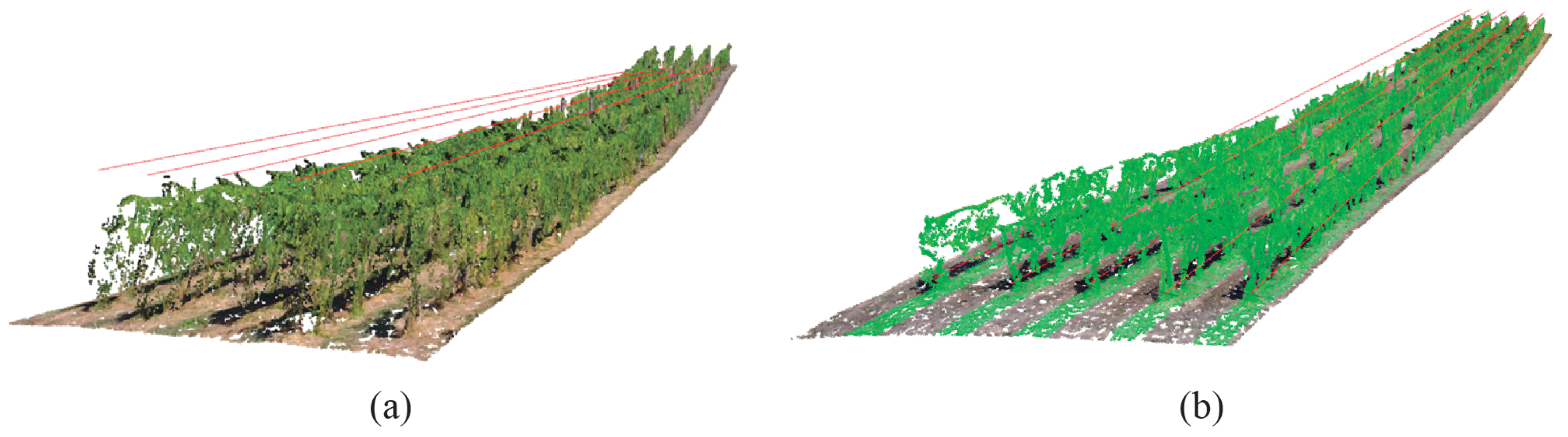
Figure 4.
Example of a segmentation of vine rows: (a) visualisation of the 3D vine rows generated as presented in Pádua et al. [14]; and (b) 3D points selection in the point cloud, using a 60 cm buffer.
Figure 4.
Example of a segmentation of vine rows: (a) visualisation of the 3D vine rows generated as presented in Pádua et al. [14]; and (b) 3D points selection in the point cloud, using a 60 cm buffer.

Figure 5.
Subdivision of the vine row into n segments.

Figure 6.
Cutting plane adjustment for the ground removal in segment n.

Figure 7.
Cutting plane adjustment for the leaves removal.

Figure 8.
Optimisation of the clustering segmentation procedure.

Figure 9.
Recognition of posts: (a) post location in the point cloud; and (b) the search of vegetation points around the trunk.
Figure 9.
Recognition of posts: (a) post location in the point cloud; and (b) the search of vegetation points around the trunk.

Figure 10.
Cases where the trunks are occluded or cannot properly modelled.

Figure 11.
Recognition of missing or occluded plants.

Figure 12.
3D model generated of the complex vineyard plot: (a) the reconstruction of study area using all the 3D points; and (b) final model, after application of noise filter.
Figure 12.
3D model generated of the complex vineyard plot: (a) the reconstruction of study area using all the 3D points; and (b) final model, after application of noise filter.

Figure 13.
Main steps for individual trunk detection: (a) ground points identification and removal, (b) vegetation/leaf points identification and removal; and (c) trunk detection.
Figure 13.
Main steps for individual trunk detection: (a) ground points identification and removal, (b) vegetation/leaf points identification and removal; and (c) trunk detection.

Figure 14.
General overview of the results obtained from the application of the proposed method to the whole complex plot. Coordinates in WGS84 (EPSG:4326).
Figure 14.
General overview of the results obtained from the application of the proposed method to the whole complex plot. Coordinates in WGS84 (EPSG:4326).

Figure 15.
Individual grapevine delineation resulting from the application of the proposed method to the validation area: (a) points to represent detected plants (visible and occluded trunks), missing plants, wrong clusters and posts; and (b) 3D point cloud and points computed for the plant location.


Table 1.
Number of plants and overall accuracy (OA) of the proposed method compared to the ground-truth data of five vine rows. Row total values—maximum possible number of plants in a given vine row—are also provided.
Table 1.
Number of plants and overall accuracy (OA) of the proposed method compared to the ground-truth data of five vine rows. Row total values—maximum possible number of plants in a given vine row—are also provided.
| Vine Row | Number of Grapevines | Missing Grapevines | Row Total | ||||||
|---|---|---|---|---|---|---|---|---|---|
| Obs. | Est. | OA (%) | Obs. | Est. | OA (%) | Obs. | Est. | OA (%) | |
| 1 | 46 | 43 | 93.5 | 12 | 15 | 75.0 | 58 | 58 | 100.0 |
| 2 | 39 | 37 | 94.9 | 18 | 21 | 83.3 | 57 | 58 | 98.2 |
| 3 | 42 | 45 | 92.9 | 15 | 12 | 80.0 | 57 | 57 | 100.0 |
| 4 | 40 | 46 | 85.0 | 17 | 9 | 52.9 | 57 | 55 | 96.5 |
| 5 | 49 | 50 | 98.0 | 7 | 7 | 100.0 | 56 | 57 | 98.2 |
| Total | 216 | 221 | 97.7 | 69 | 64 | 92.8 | 285 | 285 | 100.0 |
Table 2.
Evaluation of the proposed method in the classification grapevines and missing grapevines for the following parameters: precision, recall, F1score, and overall accuracy (OA). The ground-truth of five vine rows was used. TP: true positive; FP: false positive; TN: true negative; FN: false negative.
| Vine Row | TP | FP | TN | FN | Precision | Recall | F1score | O.A. (%) |
|---|---|---|---|---|---|---|---|---|
| 1 | 39 | 4 | 8 | 7 | 0.91 | 0.85 | 0.88 | 81.0 |
| 2 | 32 | 5 | 16 | 5 | 0.86 | 0.86 | 0.86 | 82.8 |
| 3 | 40 | 5 | 7 | 5 | 0.89 | 0.89 | 0.89 | 82.5 |
| 4 | 42 | 4 | 6 | 3 | 0.91 | 0.93 | 0.92 | 87.3 |
| 5 | 45 | 5 | 4 | 3 | 0.90 | 0.94 | 0.92 | 86.0 |
| Total | 198 | 23 | 41 | 23 | 0.90 | 0.90 | 0.90 | 83.9 |
© 2020 by the authors. Licensee MDPI, Basel, Switzerland. This article is an open access article distributed under the terms and conditions of the Creative Commons Attribution (CC BY) license (http://creativecommons.org/licenses/by/4.0/).
Share and Cite
MDPI and ACS Style
Jurado, J.M.; Pádua, L.; Feito, F.R.; Sousa, J.J. Automatic Grapevine Trunk Detection on UAV-Based Point Cloud. Remote Sens. 2020, 12, 3043. https://doi.org/10.3390/rs12183043
AMA Style
Jurado JM, Pádua L, Feito FR, Sousa JJ. Automatic Grapevine Trunk Detection on UAV-Based Point Cloud. Remote Sensing. 2020; 12(18):3043. https://doi.org/10.3390/rs12183043
Chicago/Turabian StyleJurado, Juan M., Luís Pádua, Francisco R. Feito, and Joaquim J. Sousa. 2020. "Automatic Grapevine Trunk Detection on UAV-Based Point Cloud" Remote Sensing 12, no. 18: 3043. https://doi.org/10.3390/rs12183043
Note that from the first issue of 2016, this journal uses article numbers instead of page numbers. See further details here.