The Potential of Spectral Measurements for Identifying Glyphosate Application to Agricultural Fields ^†

Abstract

Glyphosate is one of the most widely used non-selective systemic herbicides, but nowadays its application is controversially discussed. Optical remote sensing techniques might provide a sufficient tool for monitoring glyphosate use. In order to investigate the potential of this technology, a laboratory experiment was set-up using pots with rolled grass sods. Glyphosate-treated plants were compared to drought-stressed and control plants. All pots were frequently measured using a field spectrometer and a hyperspectral-imaging camera. Plant samples were analysed for photosynthetic pigments, polyphenols and dry matter content. Eight selected vegetation indices were calculated from the spectral measurements. The results show that photosynthetic pigments were sensitive to differentiate between control and glyphosate treated plants already 2 days after application. From the vegetation indices, the normalized difference lignin index (NDLI) responded most sensitively followed by indices referring to photosynthetic pigments, namely, the carotenoid reflectance index (CRI-1) and the photochemical reflectance index (PRI). It can be concluded that spectral vegetation indices are, in principal, a suitable proxy to non-destructively monitor glyphosate application on agricultural fields. Further research is needed to verify its applicability under field conditions. An operational monitoring is, however, currently limited by the requirements for temporal and spectral resolution of the satellite sensors.

1. Introduction

Glyphosate is the most widely used foliar-applied, non-selective herbicide against a broad range of different weeds. It causes nearly a direct growth inhibition, followed by chlorosis in young tissues and necrosis throughout the entire plant within 1–2 weeks after application.

Glyphosate was evaluated as a toxicologically and environmentally safe chemical, because the mode of action is restricted to plants and some microbes. An accumulation in the environment is not likely to occur as a fast-microbial degradation was observed under optimum field conditions. Therefore, glyphosate became the “world’s best-selling herbicide” after it was introduced in 1974 [1]. The application is of high relevance in no-till cropping systems and helps to reduce nutrient losses and erosion. Glyphosate application increased considerably when glyphosate-resistant, genetically modified crops were developed and which are nowadays grown in high proportions especially in the United States [2]. A further advantage of glyphosate application is the acceleration and synchronization of the ripening process of cereals that enable an economic harvest with lower losses.

The mode of action of glyphosate is an inhibition of the enzyme 5-enolpyroyl-shikimate-3-phosphate synthase (EPSPS) in the shikimate pathway that is restricted to plants and microbes, wherefore negative effects on animals and humans seemed impossible. As a result, the biosynthesis of essential aromatic amino acids (tryptophane, phenylalanine, and tyrosine) is disturbed as well as the biosynthesis of molecules that are derived from these amino acids such as phytoalexins, lignin, indoleacetic acid, tannins, anthocyanins, flavonoids, and many other compounds. As a consequence, treated plants desiccate within a short while. Not only the reduction of aromatic amino acids is responsible for this effect but also an increased carbon flow to the shikimate pathway, because of missing feedback inhibition and subsequent shortage of carbon for other pathways [1].

Once taken up by the plants via the leaf’s surface, glyphosate is quite mobile within the plant and reaches meristems, young roots and leaves, storage organs, and other growing tissue. According to Duke and Powles [1] the easy uptake, the excellent translocation to growing sites, nil or limited degradation in the plant, and a slow mode of action are the reasons for the excellent efficacy of glyphosate.

In the last couple of years, a controversial discussion came up. There is an increasing body of evidence that the chemical is negatively affecting biodiversity and wildlife, and it is under suspicion of provoking cancer in humans [3]. Due to the fact that glyphosate resistance has become a standard ingredient in genetically modified crops, gene flow of glyphosate resistance transgenes to non-transgenic crops has occurred. As a result of the extensive use of glyphosate and the high selection pressure, naturally resistant weed crops have been developed in the last several years even if it took more than 20 years since glyphosate started being used [4,5]. Already, more than 20 weed species have developed glyphosate resistance [5]. Moreover, data indicate that degradation of glyphosate is much lower in the northern hemisphere and translocation of glyphosate to non-target plants and to water bodies cannot be excluded [3]. The toxic effects of glyphosate and its degradation products have been described in bacteria and fungi [6] as well as in invertebrates and vertebrates in terrestrial and aquatic ecosystems [7,8,9,10]. Aquatic systems are especially endangered because of the high solubility of glyphosate-based formulations, and the effects on several organisms are reviewed in Helander et al. [3].

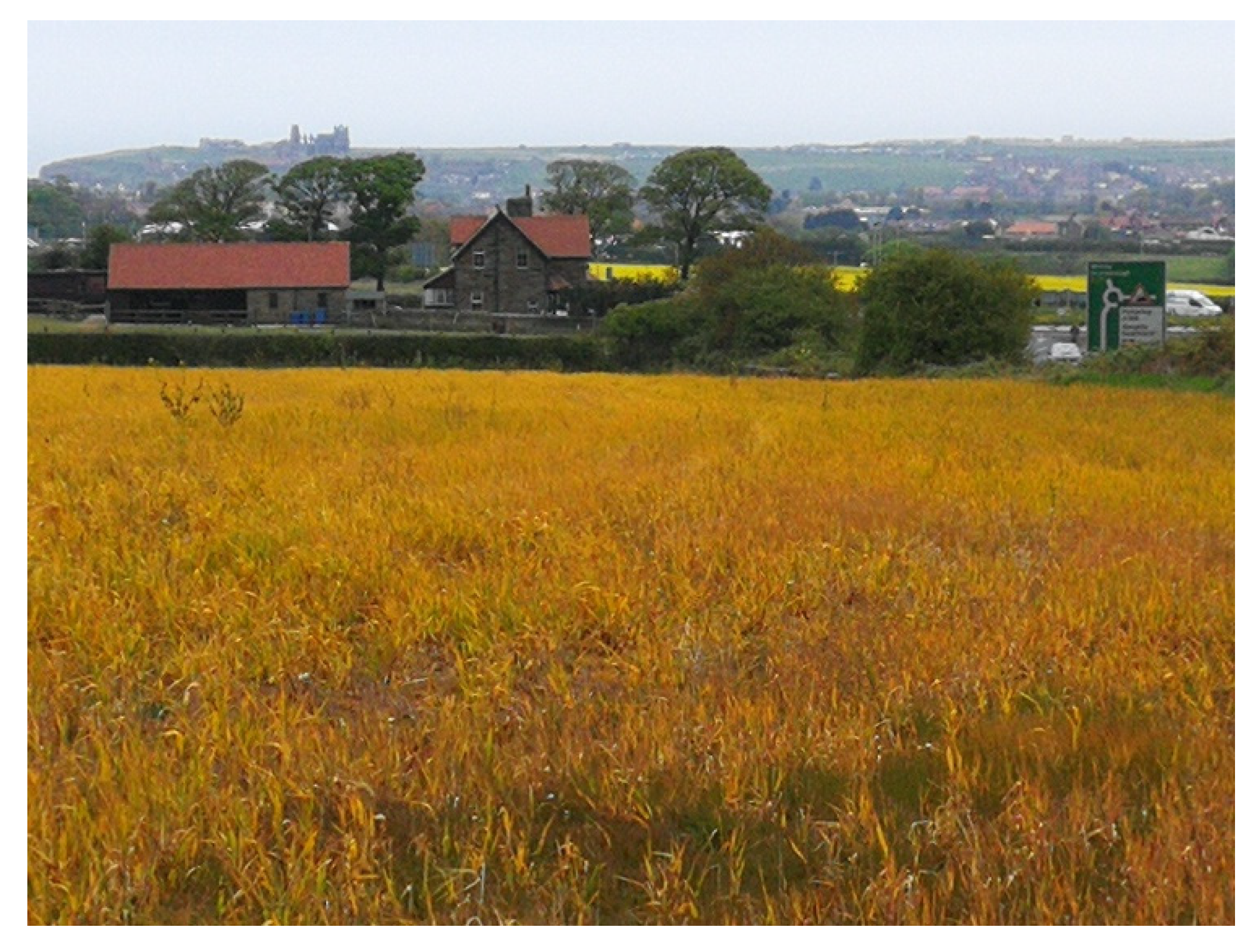
Despite the fact that the criteria for permission to use glyphosate in the EU were just recently elongated, member states can decide on their own whether glyphosate usage will be further allowed on a national level. If glyphosate application is prohibited or restricted in the future, control instruments will become important in order to monitor illegal application. Since it was observed in the past that glyphosate-treated fields show a distinctive yellowish colouring with increased magenta shares in the colour palette observed by the human eye (Figure 1), the idea arose that the spectral signature of treated fields will be specific, and it might be possible to use remote sensing techniques to monitor glyphosate application. Image analysis is already used in breeding programs to select herbicide-resistant varieties as proposed by Ali et al. [11].

It was the aim of the current study to analyse the spectral signature of glyphosate-treated plants in comparison to control plants and plants under drought stress to evaluate if there is a glyphosate-specific spectral pattern. Eight selected spectral vegetation indices were calculated from spectral measurements and their suitability for the non-destructive and rapid detection of glyphosate applications on agricultural fields was examined.

Additionally, photosynthetic pigments were analysed as compounds of the primary metabolism and measure for plant vitality and polyphenols, which are typical stress markers of the secondary plant metabolism. The dry matter content was determined as a simple attribute of plant vitality.

2. Materials and Methods

2.1. Experimental Design

Rolled grass sod of approximately 50 cm × 200 cm was purchased from Rasenland Rottdorf. The population was a mixture from 40% ryegrass (Lolium perenne L.), 40% Kentucky blue grass (Poa pratensis L.) and 20% red fescue (Festuca rubra L.) grown on a loamy sand. The rolled grass sod was cut in one direction as the width already fit with that of the containers. Each container was filled with 11.5 kg of sandy loam and the patches of grass sod with approximately 2 cm of substrate were put on top and slightly compacted and watered well to flush soil particles away from the grass sod surface.

Nine containers were prepared on 4 June 2019 and were left to grow in an open cage greenhouse with ambient air temperature and natural light until 9 July to acclimate the plants to the experimental conditions. During that time, the plants were cut 5 times to a height of 5–6 cm. The last cutting was performed on 8 July one day before the experiment started.

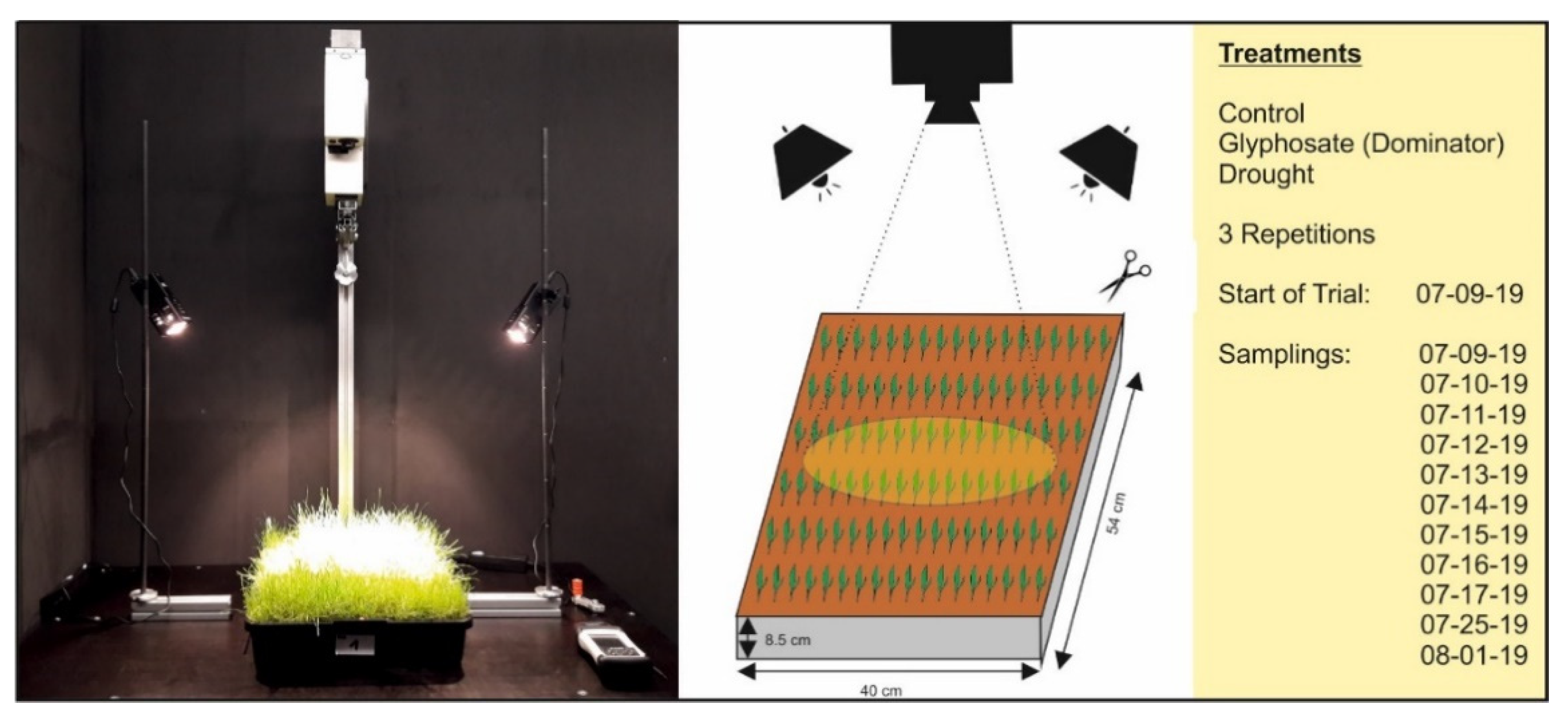
On 9 July 2019, the experiment was set-up: three of the containers were used as control and were continuously watered throughout the experiment according to the crop’s water demand. Three containers received a spray application with 13 mL glyphosate solution, which was prepared according to the instruction of the packaging for grass (Dominator 480 TF: 1 mL diluted in 100 mL of distilled water). This treatment was watered according to the crops demand, too. The last three containers were no longer watered from 9 July. All containers were observed until 1 August 2019. During this time, spectral reflectance was acquired using a field spectrometer and a hyperspectral imaging camera. Following these measurements, plant samples were taken for chemical analysis (Figure 2). Finally, growth in the containers was documented using a standard digital camera (Leica D-Lux 2).

During the first 9 days from 9 July (day 0) to 17 July (day 8) measurements were performed every day. After this period, containers were sampled two more times, on 25 July and on 1 August. This was necessary due to the considerably slower vegetation dieback of the drought treatment than of the glyphosate treatment.

2.2. Plant Sampling and Chemical Analysis

Plant samples were taken at the edges of the container to prevent disturbances of the subsequent measurements, considering that the spectral analysis was conducted in the central area. Samples were divided into sub-samples, one for the determination of photosynthetic pigments and the second one for polyphenol determination.

Photosynthetic pigments: Chlorophyll a and b, and carotenoids were determined according to Lichtenthaler [12]. About 100 mg of fresh plant material that was exactly weighted was ground and extracted with acetone (100%), whereby a pinch of CaCO₃ was added [13]. Samples were filled up with acetone to a final volume of 10 mL. The extracts were centrifuged for 5 min at 5900 rpm at room temperature. Afterwards, the absorption of the supernatant was measured at different wavelengths (645, 662, 470, 730 nm) using a UV-Vis spectrometer (Lambda-35, Perkin Elmer, Rodgau, Germany). The measurement at 730 nm should be very low and was conducted as a quality control.

The content of chlorophyll ab and carotenoids were calculated on a fresh matter basis from the measured absorption values according to Lichtenthaler and Wellburn [14] by the following equations:

$$\mathrm{Chlorophyll}a(\mathsf{\mu }\mathrm{g}/\mathrm{mL}\mathrm{plant}\mathrm{extract}) =11.75\ast A662-2.35\ast A645$$

(1)

$$\mathrm{Chlorophyll}b(\mathsf{\mu }\mathrm{g}/\mathrm{mL}\mathrm{plant}\mathrm{extract})=18.61\ast A645-3.96\ast A662$$

(2)

$$\mathrm{Carotenoids}(\mathsf{\mu }\mathrm{g}/\mathrm{mL}\mathrm{plant}\mathrm{extract})=\frac{1000\ast A470-2.27\ast \mathrm{Chl}a-81.4\ast \mathrm{Chl}b}{227}$$

(3)

Polyphenol determination: Fresh plant material was pestled to a fine powder under liquid nitrogen by a mortar. About 200 mg of the fine powder was exactly weight in Eppendorf tubes and extracted with 1 mL ethanol/water (1/1, v/v) in an ultrasonic bath for 30 min. Afterwards, the extracts were centrifuged for 15 min at 13,200 rpm and the supernatant was transferred into a tube. The extraction procedure was repeated three times and the three supernatants were combined and yielded approximately 3 mL of sample. From this sample, 1 mL was diluted with 4 mL of distilled water and from this dilution the staining was conducted in the following way:

From the diluted sample 600 µL was mixed with 3 mL of staining solution (Folin–Ciocalteu reagent (Sigma–Aldrich) which was diluted every day fresh 1:10 with distilled water) and were left for 2–4 min to react. Then 2.4 mL Na₂CO₃ solution (7.5%) was added and the tubes were mixed by inversion and left for 2 h to react at room temperature. Afterwards, the absorption was measured at 765 nm using a UV-Vis spectrometer (Lambda-35, Perkin Elmer, Rodgau, Germany). A standard calibration curve was prepared from gallic acid dissolved in water in concentrations of 10, 20, 30, 40, 50, 60 and100 mg gallic acid/l, which was stained in the same way as the samples and was used for the quantification and the total phenol content as gallic acid equivalents.

Additionally, from each plant sample, the dry matter content was determined after drying the plant material in a ventilated oven at 60 °C until constancy of weight. Therefore, it was possible to calculate the polyphenol and photosynthetic pigment content on a dry matter basis as well.

2.3. Spectral Measurements

Reflectance measurements were acquired in the laboratory with a Spectra Vista Cooperation (SVC) HR1024i field spectrometer ranging from 350 nm to 2500 nm. The SVC field spectrometer consists of three diffraction grating spectrometers ranging from 350 nm to 1000 nm, 1000 nm to 1890 nm and from 1890 nm to 2500 nm with a spectral resolution (FWHM, full width at half maximum) of ≤3.5 nm, ≤9.5 nm and ≤6.5 nm, respectively. All measurements were taken with a 14° nominal foreoptic (FOV) and a scan time of 3 s relative to a standardized Spectralon panel. Two 75 W halogen lamps mounted on either side of the spectrometer were used to illuminate the target at an incident angle of 30°. The distance between sensor and sample surface was approximately 80 cm resulting in a measurement spot diameter of about 20 cm (Figure 2).

All spectra were resampled to 1 nm and smoothed using a Savitzky Golay filter [15] with a filter size of 32 and a smoothing polynomial of 4. Before analysis, noisy bands on either side of the spectral range below 400 nm and above 2450 nm were removed.

Measurements with the SVC field spectrometer were carried out on all 11 days of the experiment. In addition, every second day starting on 9 July hyperspectral image data were acquired using a mobile hyperspectral imaging system [16]. The Specim IQ camera measures reflectance in 204 spectral bands between 400 nm and 1000 nm with a spectral resolution of 7 nm (FWHM). The camera was mounted approximately 36 cm above the pots’ surface resulting in a field of view of 20 cm × 20 cm in the centre of the pots.

2.4. Spectral Vegetation Indices

Numerous spectral vegetation indices have been reported in the literature and shown to be correlated with various vegetation parameters including plant structure, leaf pigments, biochemical composition and physiological parameters [17,18]. Their performance and sensitivity to external factors, such as illumination conditions, observation geometry or soil background, were tested in extensive studies [19]. Due to the effect of glyphosate on healthy green vegetation, eight spectral indices (

Table 1. Spectral vegetation indices evaluated in this study.

Index	Full Name	Formula (Wavelength λ in [nm])	Sensitivity	Reference
PSSRa	Pigment specific simple ratio (chlorophyll) index	(λ800/λ680)	Chlorophyll a	[20]
IRECI	Inverted red-edge chlorophyll index	(λ783 − λ665)/(λ700/λ740)	Chlorophyll	[21]
mARI	Modified anthocyanin reflectance index	(1/λ550 − 1/λ700) × λ780	Anthocyanin	[22]
CRI-1	Carotenoid reflectance index	(1/λ515 − 1/λ565) × λ790	Carotenoids	[22]
PRI	Photochemical reflectance index	(λ531 − λ570)/(λ531 + λ570)	Photosynthetic activity	[23,24]
NDLI	Normalized difference lignin index	(log(1/λ1754) − log(1/λ1680))/(log(1/λ1754) + log(1/λ1680))	Lignin	[25]
NDVI	Normalized difference vegetation index	(λ800 − λ670)/(λ800 + λ670)	Plant structure	[26]
NDWI	Normalized difference water index	(λ860 − λ1240)/(λ860 + λ1240)	Canopy water	[27]

) specifically designed to detect leaf pigments, plant water content, biochemical components and radiation use efficiency have been selected for this study. In addition, the relevance of other spectral indices was statistically tested (e.g., MTVI2—modified triangulation vegetation index; PSRI—plant senescence reflectance index). As they were less specific to build-up the plants’ glyphosate response, the data are not shown in the results section.

2.5. Statistical Analysis

A Tukey test was used for the comparison of means to determine which ones were significantly different from each other at the 5% significance level (LSD_5%). The analysis was performed using CoStat 6.451 from CoHort software (Informer Technologies, Inc., Los Angeles, CA, USA).

To analyse the relationship between the chemical parameters and the spectral vegetation indices, linear regression models were set-up using lm function in R version 3.6.2.

3. Results

3.1. Photo-Optical Documentation

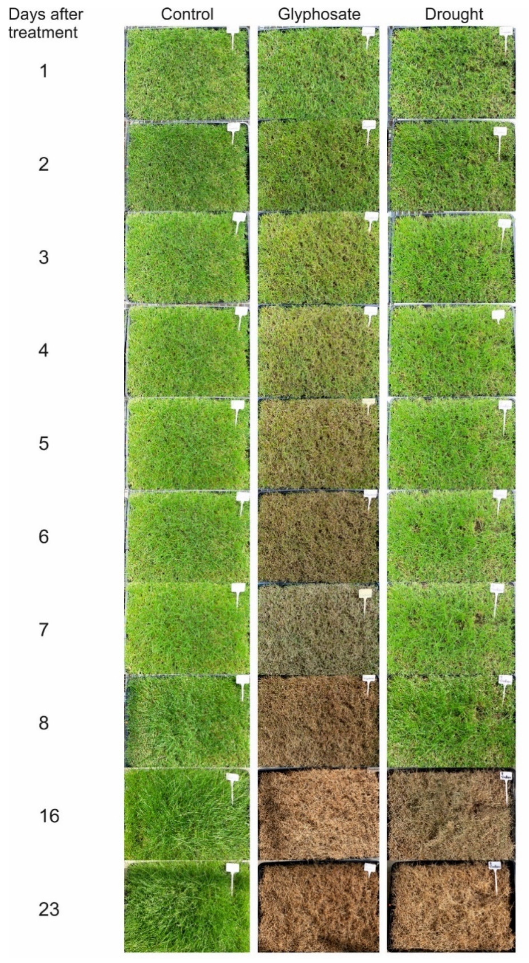
The photo-optical documentation (Figure 3) of the development of treated containers in comparison to the control over the experimental time revealed that glyphosate caused a change in colour already 3 days after spray application. After 6–7 days, glyphosate treatment caused dieback of the grass. During the experiment, many challenges were encountered such that one of the three glyphosate-treated containers reacted with a time lag and showed visual symptoms starting on day 6. Eight days after application, the three glyphosate-treated containers showed a comparable appearance. These differences in dieback had a strong effect on the statistics. Despite strong differences between the control and the glyphosate treatment in many of the investigated parameters, these differences became significant only later in the experiment. The drought treatment reacted very slowly because a lot of water was stored in the grass sod. Therefore, it was necessary to elongate the experimental time to show the effect of drought on the investigated parameters. The dry matter content of the control plants and the drought plants was still comparable on day 8 of the experiment (

Table 2. Tukey’s test statistics of the chemical grass composition of control (Ctr) plants at each sampling on a fresh matter (FM) basis in relation to glyphosate (Gly) and drought (Dry) treatment.

DAA	Treatment	DM	Chla	Chlb	Chlab	Car	PP
		(%)	(mg/g FM)
0	Ctr	19.0 a	1.14 a	0.247 a	1.39 a	0.417 a	0.74 a
	Gly	18.3 a	1.08 a	0.234 a	1.31 a	0.403 a	0.80 a
	Dry	18.7 a	1.09 a	0.242 a	1.34 a	0.407 a	0.98 a
	LSD5%	3.5	0.31	0.068	0.38	0.102	0.27
1	Ctr	17.7 a	1.00 a	0.209 a	1.21 a	0.366 a	0.99 a
	Gly	17.0 a	0.93 a	0.200 a	1.13 a	0.346 a	1.01 a
	Dry	16.6 a	1.02 a	0.210 a	1.23 a	0.374 a	0.88 a
	LSD5%	2.7	0.20	0.047	0.25	0.063	0.49
2	Ctr	17.5 a	1.27 a	0.259 a	1.53 a	0.486 a	0.84 a
	Gly	17.1 a	0.98 b	0.213 a	1.19 b	0.396 b	0.61 a
	Dry	15.4 a	1.18 ab	0.237 a	1.42 ab	0.452 ab	0.80 a
	LSD5%	3.1	0.17	0.041	0.21	0.063	0.28
3	Ctr	16.9 a	1.37 a	0.288 a	1.66 a	0.503 a	0.93 a
	Gly	18.9 a	1.01 b	0.228 a	1.23 a	0.403 a	0.72 a
	Dry	16.7 a	1.08 ab	0.227 a	1.30 a	0.397 a	0.92 a
	LSD5%	3.1	0.28	0.066	0.34	0.112	0.39
4	Ctr	17.2 a	1.45 a	0.305 a	1.75 a	0.526 a	0.88 a
	Gly	20.8 a	0.93 b	0.206 b	1.14 b	0.383 b	0.78 a
	Dry	17.1 a	1.39 a	0.288 a	1.67 a	0.504 a	1.12 a
	LSD5%	3.2	0.23	0.049	0.29	0.084	0.54
5	Ctr	17.9 a	1.43 a	0.296 a	1.72 a	0.505 a	0.84 a
	Gly	30.6 a	1.08 a	0.247 a	1.33 a	0.466 a	1.13 a
	Dry	18.5 a	1.34 a	0.276 a	1.62 a	0.473 a	0.90 a
	LSD5%	10.8	0.46	0.107	0.56	0.199	0.56
6	Ctr	16.5 a	1.48 a	0.310 a	1.79 a	0.526 a	1.02 a
	Gly	38.7 a	1.09 a	0.257 a	1.35 a	0.466 a	1.25 a
	Dry	17.4 a	1.39 a	0.292 a	1.68 a	0.498 a	0.79 a
	LSD5%	18.7	0.37	0.094	0.460	0.161	0.63
7	Ctr	17.1 b	1.68 a	0.358 a	2.04 a	0.601 a	0.81 b
	Gly	50.6 a	0.86 c	0.237 b	1.10 c	0.374 c	1.76 a
	Dry	16.8 b	1.41 b	0.302 a	1.72 b	0.503 b	0.93 b
	LSD5%	18.2	0.19	0.050	0.25	0.061	0.65
8	Ctr	17.8 b	1.54 a	0.330 a	1.87 a	0.546 a	0.92 b
	Gly	62.9 a	0.68 b	0.199 b	0.88 b	0.292 b	2.16 a
	Dry	17.3 b	1.54 a	0.336 a	1.87 a	0.536 a	1.25 b
	LSD5%	16.3	0.33	0.063	0.39	0.140	0.51
16	Ctr	18.9 b	1.93 a	0.460 a	2.40 a	0.711 a	1.31 b
	Gly	90.7 a	0.01 b	0.005 b	0.02 b	0.008 c	3.83 a
	Dry	92.5 a	1.37 a	0.564 a	1.94 a	0.433 b	3.67 a
	LSD5%	1.5	0.58	0.207	0.78	0.181	0.37
23	Ctr	20.4 b	2.11 a	0.514 a	2.62 a	0.770 a	1.65 b
	Gly	86.5 a	0.01 b	0.003 b	0.01 b	0.006 b	3.56 a
	Dry	87.2 a	0.05 b	0.026 b	0.07 b	0.023 b	3.87 a
	LSD5%	0.7	0.16	0.055	0.21	0.036	0.58

DAA = days after application, Chla = chlorophyll a, Chlb = chlorophyll b, Chlab = total chlorophyll, Car = carotenoids, PP = polyphenols, LSD = least significant difference. Different letters behind parameters printed in bold indicate to statistically significant different mean values at the 5% significance level by Tukey’s test in comparison to the control at that date.

).

Figure 3 demonstrate the problem that the visual impression of photograph pictures depends very much on light conditions and can vary with daylight. This is the reason why it was necessary to perform the investigation under controlled light conditions in a darkroom. The pictures in Figure 3 shall only serve as a visualization of the trial.

3.2. Statistical Analysis of Chemical Compounds

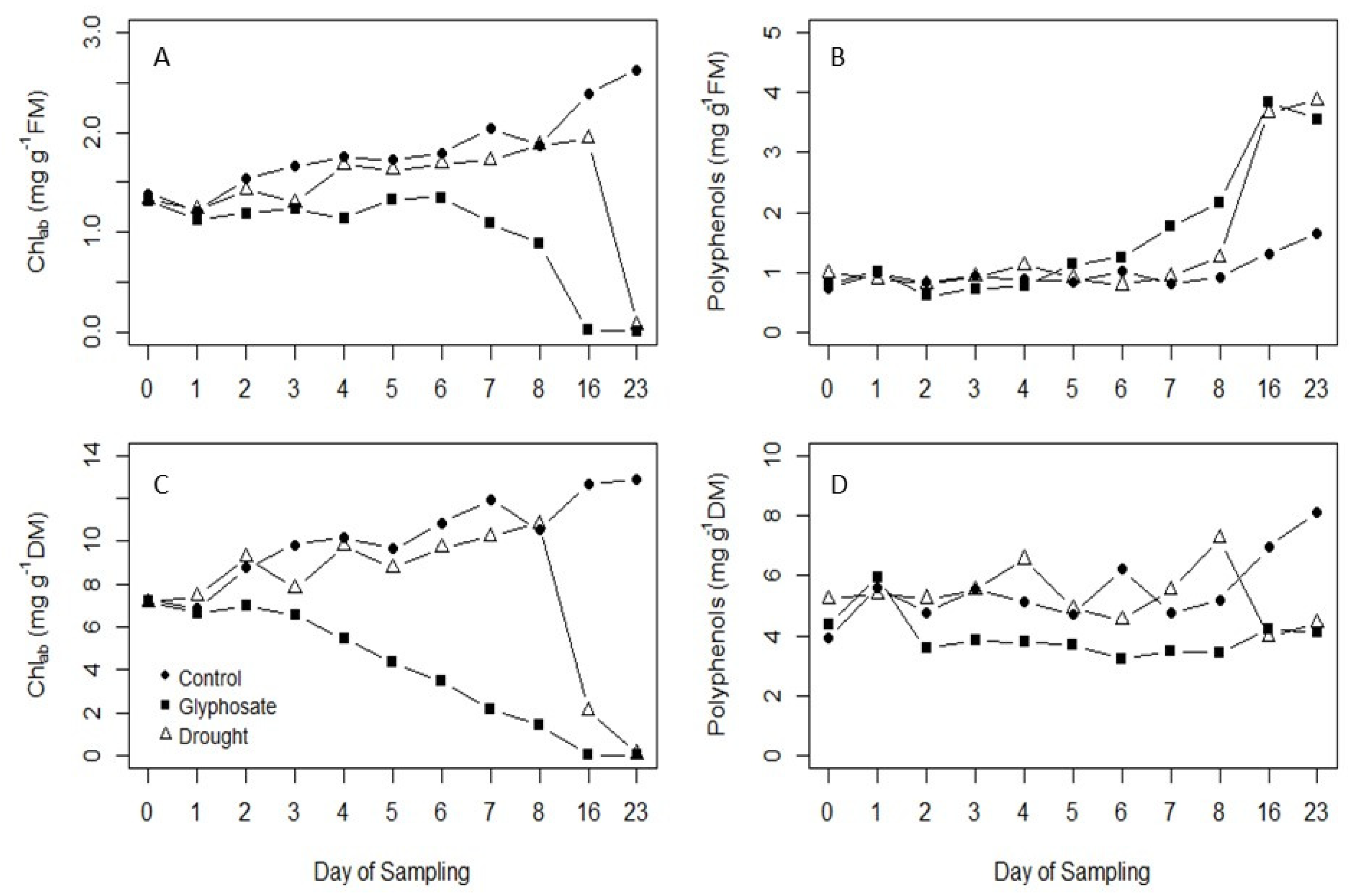
The data in Table 2 demonstrate that chlorophyll a, total chlorophyll ab and carotenoids were already significantly reduced in glyphosate-treated plants 2 days after application. However, no changes were visible to the human eye at that time (Figure 3). The polyphenols increased in the glyphosate-treated plants from day 5 on (Figure 4B) and the increase was statistically significant on day 7 (Table 2). A stress-related increase in the polyphenol content was observed under drought stress conditions only at the last two samplings when also the pigment content was reduced. The dry matter content increased with glyphosate treatment and drought as well. Therefore, it is important to analyse the data on a dry matter basis as well to show if changes were caused by a loss of water or if changes occurred in plant metabolism (

Table 3. Tukey’s test statistics of the chemical grass composition of control (Ctr) plants at each sampling on a dry matter (DM) basis in relation to glyphosate (Gly) and drought (Dry) treatment.

DAA	Treatment	Chla	Chlb	Chlab	Car	PP
		(mg/g DM)
0	Ctr	5.95 a	1.29 a	7.25 a	2.18 a	3.93 a
	Gly	5.91 a	1.29 a	7.20 a	2.21 a	4.37 a
	Dry	5.88 a	1.29 a	7.17 a	2.18 a	5.29 a
	LSD5%	1.12	0.25	1.37	0.36	1.83
1	Ctr	5.73 a	1.19 a	6.92 a	2.09 a	5.50 a
	Gly	5.45 a	1.17 a	6.62 a	2.03 a	5.95 a
	Dry	6.16 a	1.26 a	7.42 a	2.26 a	5.30 a
	LSD5%	1.13	0.25	1.37	0.34	2.15
2	Ctr	7.30 a	1.48 a	8.79 a	2.79 ab	4.85 a
	Gly	5.75 b	1.25 b	7.00 b	2.33 b	3.56 a
	Dry	7.71a	1.55 a	9.26 a	2.95 a	5.29 a
	LSD5%	1.03	0.18	1.22	0.40	2.20
3	Ctr	8.11 a	1.70 a	9.81 a	2.97 a	5.54 a
	Gly	5.36 b	1.21 b	6.58 b	2.15 b	3.87 a
	Dry	6.44 b	1.36 ab	7.80 b	2.38 ab	5.50 a
	LSD5%	1.29	0.29	1.57	0.53	2.16
4	Ctr	8.40 a	1.77 a	10.17 a	3.06 a	5.04 a
	Gly	4.53 b	1.00 b	5.53 b	1.86 b	3.79 a
	Dry	8.14 a	1.70 a	9.83 a	2.96 a	6.61 a
	LSD5%	1.42	0.29	1.70	0.52	3.05
5	Ctr	7.96 a	1.65 a	9.61 a	2.81 a	4.65 a
	Gly	3.53 b	0.80 b	4.33 b	1.50 b	3.65 a
	Dry	7.39 a	1.52 a	8.91 a	2.60 a	4.90 a
	LSD5%	1.54	0.32	1.88	0.55	1.52
6	Ctr	8.98 a	1.88 a	10.88 a	3.19 a	6.22 a
	Gly	3.12 b	0.71 b	3.84 b	1.32 b	3.27 b
	Dry	8.02 a	1.68 a	9.69 a	2.87 a	4.64 a
	LSD5%	1.59	0.28	1.86	0.61	2.03
7	Ctr	9.84 a	2.10 a	11.93 a	3.52 a	4.78 a
	Gly	1.88 b	0.52 b	2.40 b	0.82 b	3.54 a
	Dry	8.43 a	1.80 a	10.23 a	3.00 a	5.55 a
	LSD5%	1.16	0.30	1.46	0.47	2.59
8	Ctr	8.66 a	1.85 a	10.52 a	3.07 a	5.18 b
	Gly	1.18 b	0.33 b	1.51 b	0.51 b	3.45 c
	Dry	8.87 a	1.94 a	10.80 a	3.09 a	7.25a
	LSD5%	0.91	0.18	1.07	0.37	0.57
16	Ctr	10.21 a	2.43 a	12.64 a	3.76 a	6.99 a
	Gly	0.01 c	0.01 c	0.02 c	0.01 c	4.23 b
	Dry	1.48 b	0.61 b	2.09 b	0.47 b	3.97 b
	LSD5%	1.10	0.34	1.44	0.33	1.33
23	Ctr	10.36 a	2.53 a	12.89 a	3.78 a	8.09 a
	Gly	0.01 b	0.003 b	0.01 b	0.01 b	4.11 b
	Dry	0.05 b	0.033 b	0.08 b	0.02 b	4.43 b
	LSD5%	0.95	0.306	1.25	0.23	1.90

DAA = Days after application, Chla = chlorophyll a, Chlb = chlorophyll b, Chlab = total chlorophyll, Car = carotenoids, PP = polyphenols, LSD = least significant difference. Different letters behind parameters printed in bold indicate statistically significant different mean values at the 5% significance level by Tukey’s test in comparison to the control at that date.

).

Trends are even stronger when the statistics are calculated on a dry matter basis. Photosynthetic pigments, both chlorophyll a and b as well as total chlorophyll, were reduced under glyphosate treatment already two days after application. Polyphenols were strongly related to the dry matter content and behave different when analysed on a dry matter basis (Figure 4D); while polyphenols increased with glyphosate application on fresh matter basis (Table 2, Figure 4B), a decrease was observed on dry matter basis which was significant 6 days after glyphosate application (Table 3). Therefore, it is important to record the development of the dry matter content in experiments where plants were exposed to stress.

This different trend between chlorophyll and polyphenols is also clear when comparing the development of the chlorophyll and polyphenol content over the experimental time on fresh and dry matter basis (Figure 4A–D). In case of chlorophyll, the same trend is visible on fresh and dry matter basis, which is even more pronounced when looking at the dry matter data. A different result was found for the polyphenols: a clear increase in the polyphenols was found under stress conditions with time when the results are shown on fresh matter basis while no specific trend can be recorded from the data on dry matter basis. The polyphenol content is highly correlated with the dry matter content (r² = 91%) and is therefore mainly reflecting the loss of water with drought stress and glyphosate treatment.

3.3. Spectral Reflectance Measurements

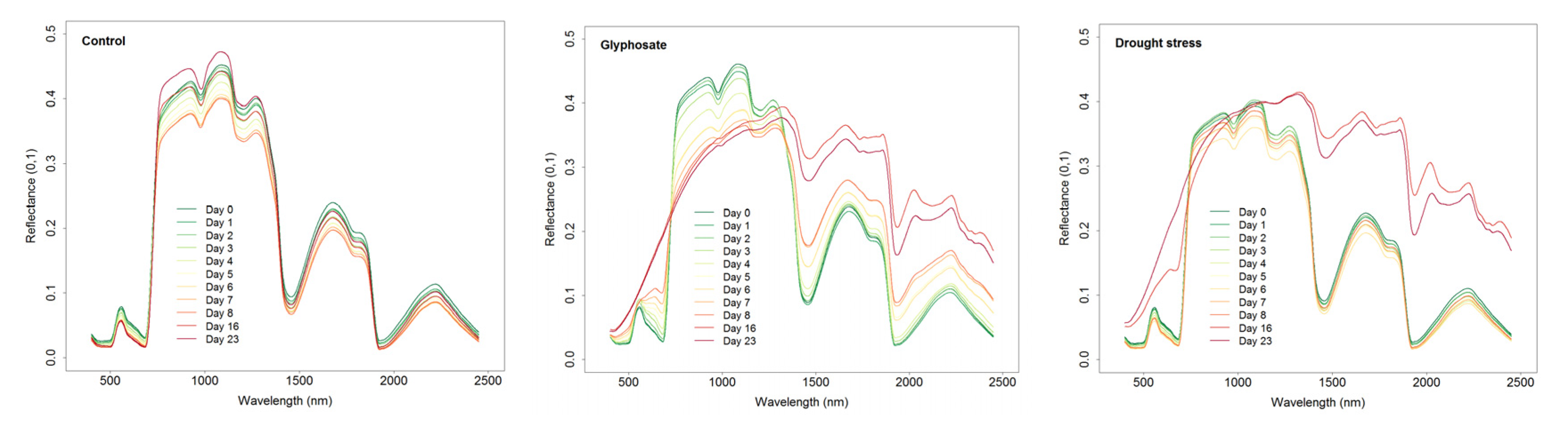
Figure 5 shows the mean reflectance spectra of the three treatments over time as recorded by the SVC field spectrometer. In accordance with results of the chemical analysis, alterations of the spectral reflectance of the glyphosate treatment became evident on day 2, i.e., the third day of the experiment. In the course of time, spectral reflectance of the glyphosate-treatments changed considerably. It increased in the visible (VIS) and in the shortwave-infrared (SWIR) part of the spectrum while reflection in the near-infrared (NIR) decreased. The grass sod under drought stress exhibited distinct changes at the last two sampling dates just as it was observed with the photosynthetic pigments and the phenols. The spectral signal of these samples was very similar to the spectral signal of the glyphosate-treated samples at these days (day 16, day 23) (Figure 6). The control showed only minor variations during the experiment. A slight increase in reflectance was detected in the NIR on day 16 and 23 when the chlorophyll and carotenoid content was the highest (Table 2, Figure 4A,C).

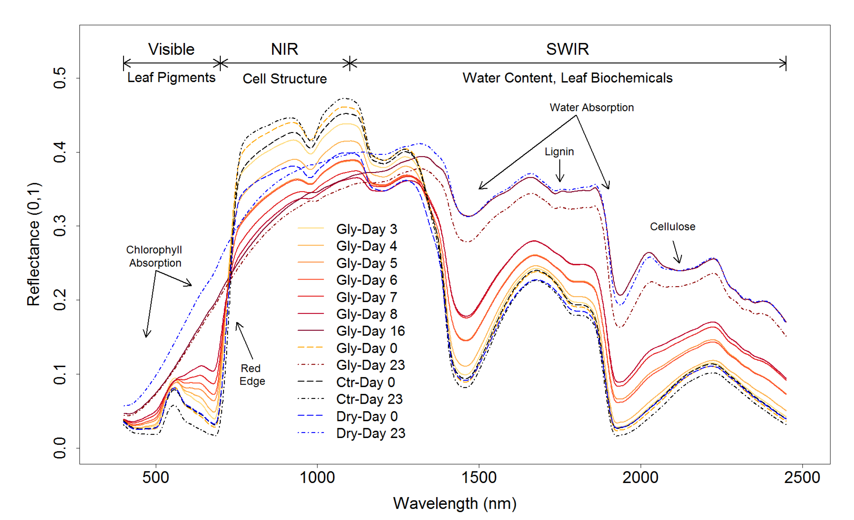
The changes in the spectral signal of the treatments can be clearly attributed to alterations of the structural and chemical characteristics of plants (Figure 6). In the VIS, the reflectance of plants is mainly controlled by leaf pigments, which strongly absorb light. The decrease of the chlorophyll and carotenoid content due to the glyphosate treatment led to a continuous decrease of absorption in this part of the spectrum. Reflectance in the NIR is determined by the cell structure. The scattering process at the air/water interfaces at the surface of cells results in a high reflection of the incident radiation. It declines with a degradation of cell structure caused by glyphosate application. In the SWIR, reflectance of green vegetation is generally low due to the high plant water content. The signal was dominated by two strong water absorption bands near 1400 nm and 1940 nm. With the dieback of vegetation, the reflectance increased as plant water decreased. Absorption bands of biochemical compounds such as lignin and cellulose, which were masked by water before, became visible.

3.4. Spectral Vegetation Indices

From the SVC reflectance data, eight spectral vegetation indices (see Table 1) were calculated to investigate if these data are suitable to distinguish between crops treated with glyphosate and those suffering from drought stress in comparison to healthy control plants.

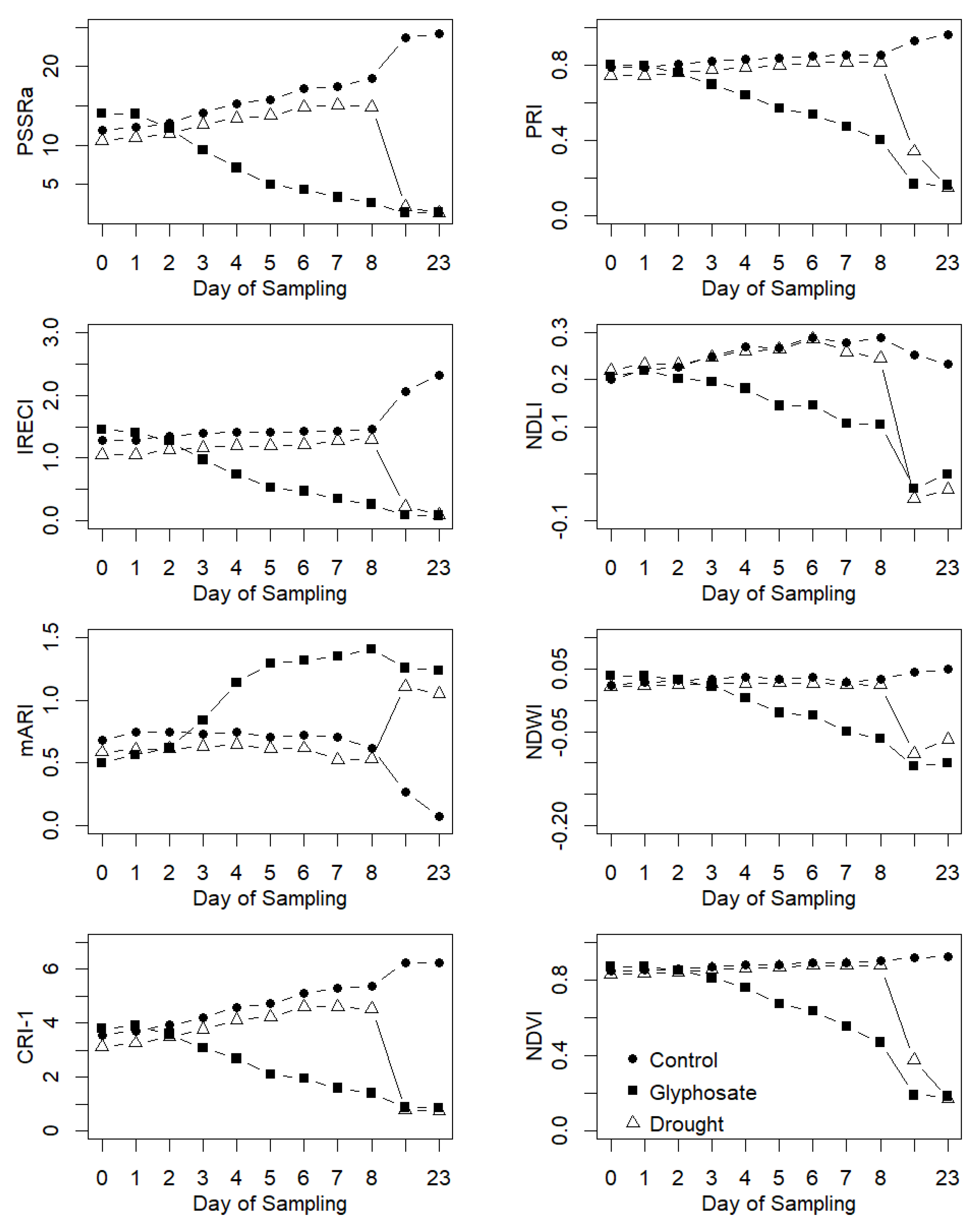
The development of the spectral vegetation indices during the course of the experiment is displayed in Figure 7; PRI, IRECI, NDVI and NDWI showed very similar trends for the control and the drought treatments up to and including day 8. Differences became visible only on the last two days of sampling. The NDLI, mARI and CRI-1 exhibited the first differences between the control and drought on day 7, whereas PSSRa on day 8. In contrast, glyphosate treatment differed already a few days after application. For NDLI, differences became obvious on day 2. The CRI-1, PRI, PSSRa and mARI indicated changes on day 3, NDWI and NDVI on day 4.

Statistical analysis using Tukey’s test (

Table 4. Tukey’s test statistics of the spectral vegetation indices of the three treatments: control (Ctr), glyphosate (Gly) and drought (Dry).

DAA	Treatment	Spectral Vegetation Indices *
		PSSRa	IRECI	mARI	CRI-1	PRI	NDLI	NDVI	NDWI
0	Ctr	12.0 a	1.31 a	0.66 a	3.57 a	0.79 a	0.20 a	0.85 a	0.30 a
	Gly	14.6 a	1.49 a	0.47 a	3.81 a	0.80 a	0.21 a	0.87 a	0.32 a
	Dry	10.6 a	1.05 a	0.59 a	3.14 a	0.74 a	0.22 a	0.83 a	0.28 a
	LSD5%	5.7	0.69	0.34	0.89	0.10	0.02	0.05	0.07
1	Ctr	12.3 a	1.31 a	0.73 a	3.71 a	0.79 a	0.22 a	0.85 a	0.31 a
	Gly	14.7 a	1.44 a	0.52 a	3.94 a	0.80 a	0.22 a	0.87 a	0.33 a
	Dry	10.9 a	1.05 a	0.60 a	3.26 a	0.75 a	0.23 a	0.84 a	0.29 a
	LSD5%	6.4	0.68	0.34	1.05	0.10	0.02	0.05	0.07
2	Ctr	12.9 a	1.38 a	0.73 a	3.92 a	0.80 a	0.23 a	0.86 a	0.32 a
	Gly	13.0 a	1.31 a	0.58 a	3.64 a	0.76 a	0.20 a	0.85 a	0.31 a
	Dry	11.5 a	1.12 a	0.61 a	3.50 a	0.76 a	0.23 a	0.84 a	0.29 a
	LSD5%	6.5	0.72	0.31	1.06	0.10	0.03	0.06	0.08
3	Ctr	14.2 a	1.42 a	0.71 a	4.20 a	0.82 a	0.25 a	0.87 a	0.33 a
	Gly	10.6 a	1.03 a	0.77 a	3.15 a	0.69 a	0.20 b	0.81 a	0.28 a
	Dry	12.7 a	1.17 a	0.63 a	3.77 a	0.78 a	0.25 a	0.86 a	0.30 a
	LSD5%	7.0	0.74	0.40	1.13	0.12	0.03	0.09	0.10
4	Ctr	15.4 a	1.44 a	0.73 a	4.59 a	0.83 a	0.27 a	0.88 a	0.34 a
	Gly	8.4 a	0.80 a	1.04 a	2.77 b	0.63 b	0.18 b	0.75 a	0.24 a
	Dry	13.5 a	1.19 a	0.64 a	4.11 ab	0.79 ab	0.26 a	0.86 a	0.30 a
	LSD5%	7.3	0.76	0.50	1.34	0.15	0.04	0.13	0.13
5	Ctr	16.0 a	1.43 a	0.68 ab	4.72 a	0.84 a	0.27 a	0.88 a	0.33 a
	Gly	6.3 b	0.60 a	1.19 a	2.22 b	0.56 b	0.15 b	0.66 a	0.16 a
	Dry	13.9 a	1.20 a	0.61 b	4.25 a	0.80 a	0.27 a	0.87 a	0.30 a
	LSD5%	6.9	0.73	0.42	1.53	0.18	0.07	0.19	0.18
6	Ctr	17.4 a	1.46 a	0.69 b	5.09 a	0.85 a	0.29 a	0.89 a	0.34 a
	Gly	5.5 b	0.53 b	1.23 a	2.05 b	0.53 b	0.15 b	0.62 b	0.16 a
	Dry	15.0 a	1.21 ab	0.61 b	4.61 a	0.81 a	0.29 a	0.88 ab	0.30 a
	LSD5%	6.6	0.71	0.41	1.50	0.19	0.08	0.21	0.17
7	Ctr	17.5 a	1.46 a	0.68 b	5.28 a	0.85 a	0.28 a	0.89 a	0.33 a
	Gly	4.1 b	0.39 b	1.29 a	1.69 b	0.46 b	0.11 b	0.55 b	0.10 b
	Dry	15.3 a	1.28 a	0.52 b	4.61 a	0.82 a	0.26 a	0.88 a	0.29 a
	LSD5%	5.4	0.63	0.37	1.29	0.19	0.07	0.22	0.15
8	Ctr	18.6 a	1.49 a	0.60 b	5.39 a	0.85 a	0.29 a	0.90 a	0.34 a
	Gly	3.0 b	0.28 b	1.38 a	1.45 b	0.40 b	0.11 b	0.47 b	0.08 b
	Dry	15.0 a	1.30 a	0.53 b	4.53 a	0.81 a	0.25 a	0.88 a	0.29 a
	LSD5%	4.5	0.57	0.23	1.07	0.17	0.04	0.21	0.12
16	Ctr	24.0 a	2.08 a	0.26 c	6.27 a	0.93 a	0.25 a	0.92 a	0.35 a
	Gly	1.4 b	0.09 b	1.26 a	0.88 b	0.17 c	−0.03 b	0.19 c	−0.07 b
	Dry	2.1 b	0.22 b	1.11 b	0.79 b	0.34 b	−0.05 b	0.38 b	−0.05 b
	LSD5%	4.1	0.35	0.12	0.68	0.06	0.03	0.03	0.04
23	Ctr	24.4 a	2.34 a	0.07 c	6.27 a	0.96 a	0.23 a	0.92 a	0.36 a
	Gly	1.4 b	0.08 b	1.24 a	0.87 b	0.16 b	0.00 b	0.19 b	−0.06 b
	Dry	1.4 b	0.10 b	1.05 b	0.76 b	0.15 b	−0.03 b	0.17 b	−0.01 b
	LSD5%	4.2	0.41	0.08	0.82	0.06	0.03	0.02	0.05

DAA = Days after application, LSD = least significant difference. Different letters in bold indicate to statistically different mean values at the 5% significance level by Tukey’s test in comparison to the control on that day. * Indices are explained in Table 1.

) confirmed the different capacity of the spectral indices to differentiate between the control plants and the glyphosate treatment. The statistics revealed that significant differences between control and glyphosate treatment existed earliest on day 3, and latest on day 7. The indices responded in the following order: NDLI (3) > CRI-1 = PRI (4) > PSSRa (5) > IRECI = mARI = NDVI (6) > NDWI (7) with NDLI differentiating first already 3 days after glyphosate application and NDWI differentiating last with 7 days after application. With respect to drought, no differences were observed. This is likely due to the fact that water shortage had an effect on the development of the sod only very late. At this time, no more daily measurements were analysed. Only one index, the mARI, was able to differentiate between glyphosate and drought treatment at the last sampling date, when all other indices showed no statistically different values.

Linear regression models were set--up to analyse the interrelationship between chemical parameters and the spectral vegetation indices (

Table 5. Coefficient of determination (R²) and significance level (Sig.) between the chemical parameters and the spectral vegetation indices (n = 99).

Spectral Index	Dry Matter (%)		Chlorophyll ab (mg/g DM)		Carotenoids (mg/g DM)		Polyphenols (mg/g DM)
	R2	Sig.	R2	Sig.	R2	Sig.	R2	Sig.
PSSRa	0.55	***	0.80	***	0.79	***	0.31	***
IRECI	0.56	***	0.71	***	0.72	***	0.28	***
mARI	0.46	***	0.63	***	0.62	***	0.32	***
CRI-1	0.63	***	0.87	***	0.86	***	0.31	***
PRI	0.86	***	0.85	***	0.87	***	0.22	***
NDLI	0.91	***	0.79	***	0.82	***	0.15	***
NDVI	0.93	***	0.78	***	0.82	***	0.16	***
NDWI	0.88	***	0.72	***	0.75	***	0.19	***

Sig. = Significance code; *** p < 0.001.

). The results showed that all relationships were highly significant but the strength of correlation as indicated by the coefficient of determination varied considerably. Generally, R² was higher for the linear models between the spectral indices and the photosynthetic pigments than for the polyphenols. With regard to the photosynthetic pigments (carotenoids, chlorophyll), the highest R² was found for CRI-1 and PRI (R² > 0.85). Scatterplots between spectral indices and plant pigments disclosed a positive linear relationship for CRI-1 and chlorophyll ab as well as CRI-1 and carotenoids, whereas PRI exhibited a sigmoid curve shape (not shown). For the polyphenols highest R² was retrieved using mARI indicating a broad scatter and a weak correlation (R² = 0.32). Furthermore, strong linear relationships were found between the dry matter content and the NDVI, NDLI, NDWI and PRI (R² > 0.86).

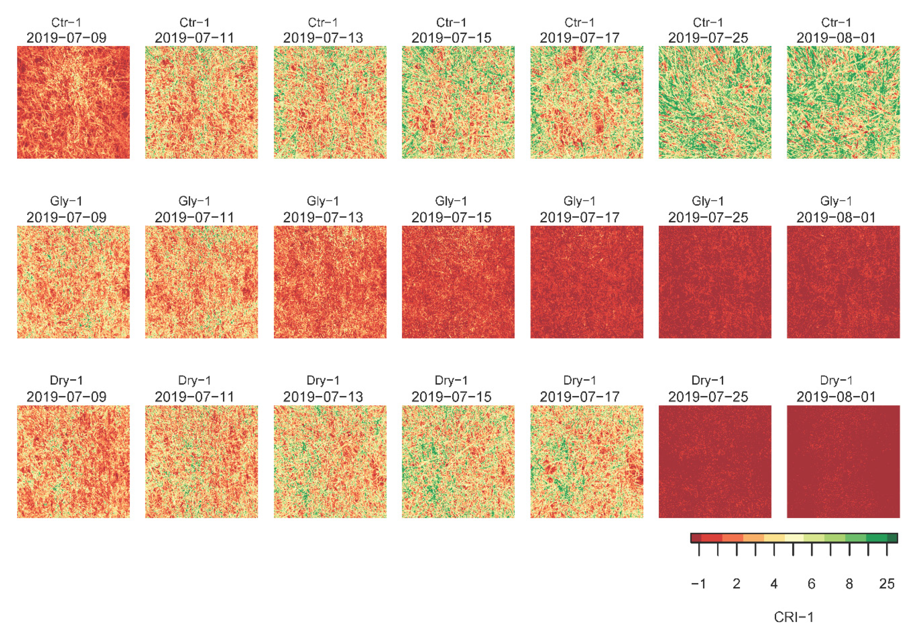
Hyperspectral image data were processed and spectral vegetation indices were calculated for each replication and date. This was done for all indices except NDWI and NDLI as these indices require data outside the wavelength range of the Specim IQ camera. The results confirmed findings obtained from the SVC reflectance measurements. The CRI-1 and PRI are the first to recognize changes after glyphosate application. Figure 8 displays the CRI-1 of the first replication for all three treatments. The index revealed first signs of deterioration already on day 2. Distinct differences between glyphosate application and the other treatments became obvious on day 4. From then on, vegetation dieback progressed rapidly. On day 16 and day 23, the glyphosate and drought treatment looked alike just as it was observed with the SVC reflectance data. Using image data, however, spatial patterns caused by the different development or dieback of the plants are additionally revealed. Finally, CRI-1 based on hyperspectral image data revealed differences in the health status of plants at the beginning of the experiment which were not visible to the naked eye.

4. Discussion

Many different factors affect the appearance of agricultural crops and cause changes in the reflectance signal of the canopy. Reasons can be manifold. There are naturally occurring processes, such as ripening or senescence but also plant diseases, plant stress like drought or salt stress as well, as treatment with herbicides such as glyphosate or weather events such as hail damage. An early differentiation between these very different processes that is quick and easy to perform and to process would be useful for the right action to be taken. Remote sensing techniques can be used for different purposes such as evaluation of weed infestation, nutrient deficiency, diseases or drift from herbicide treatment [28,29,30]. Therefore, the question arises if it may also be an appropriate method to detect vegetation dieback caused by glyphosate application.

In the present study, the effect of glyphosate application on spectral vegetation indices was investigated as a specific colouring was observed under field conditions (Figure 1) which was attributed to glyphosate. The observed chlorosis implies that a loss of photosynthetic pigments could be the main reason causing the discolouring of the plant cover but other factors may be relevant as well.

4.1. Change in Primary and Secondary Metabolism Caused by Glyphosate Treatment

The mode of action of glyphosate is an inhibition of the 5-enolpyruvylshikimate-3-phosphate synthetase in the shikimate pathway, which interferes in the production of proteins and other molecules that require the aromatic amino acids tryptophan, tyrosine or phenylalanine as precursors [3]. Aromatic amino acids are important precursors for many different compounds belonging to the primary and secondary plant metabolism, such as growth promotors like indoleacetic acid, tannins, anthocyanins, flavonoids and lignin. The disturbance in the metabolism of aromatic amino acids result in the very quick dieback of plants. It was assumed that the photosynthetic pigments and the polyphenols are good indicators to observe the changes caused by glyphosate application on a metabolic level.

Also, other studies revealed that glyphosate and its main degradation product aminomethylphosphonic acid (AMPA) caused a disturbance in the chlorophyll biosynthesis of non-resistant species, which led to decreased chlorophyll contents and a decreased photosynthetic activity in conjunction with oxidative stress [31,32]. In the present study, a clear effect of glyphosate-treatment on chlorophyll ab and carotenoids was found, too. Already 2 days after glyphosate application the contents of photosynthetic pigments decreased significantly (Table 2 and Table 3). Therefore, spectral indices that refer to the chlorophyll content or the photosynthetic activity seem to be good candidates to recognize changes caused by glyphosate application at an early stage.

Polyphenols are ubiquitous products of the secondary plant metabolism with very diverse functions including formation of pigments in flowers and fruits, a contribution to biotic and abiotic stress tolerance, pollen fertility, structural roles and signalling [33]. The main classes of polyphenols that can be commonly found in plants are flavonoids, tannins, phenolic acids, stilbenes and lignans [34], and their biosynthesis is steeply increasing under stress conditions [35,36]. According to Di Ferdinando et al. [36], polyphenols are “the most versatile secondary metabolites, thus allowing plants to respond promptly to unpredictable stress”. Phenolic compounds are defence compounds, which are produced to protect plants from herbivores or photo-damage mainly by their high antioxidant activity [37]. Under stress conditions, reactive oxygen species (ROS) can be produced which need to be detoxified to prevent plants from being damaged. Polyphenols are very active metabolites [34,35]. When chlorophyll biosynthesis is disturbed through glyphosate application, absorbance of light energy by photosynthetic pigments is disturbed, resulting in an excess of light energy, which can enhance the production of ROS. Therefore, as glyphosate application affects chlorophyll biosynthesis, limited photosynthesis will increase oxidative stress and an increase in polyphenols can be expected. Gomes et al. [31] observed a decrease in chlorophyll biosynthesis with glyphosate as well as AMPA application and both chemicals induced ROS accumulation. On the other hand, the shikimate pathway, which is disturbed by glyphosate application, is important in the biosynthesis of polyphenols. From the data (Table 2 and Table 3), it is obvious that polyphenols increased with glyphosate application, but they react much slower than photosynthetic pigments. Differences were significant only 6 to 7 days after application. Nevertheless, spectral indices that capture changes in polyphenols are also interesting for the prediction of plant stress.

The third parameter that was investigated in the plant material in the current experiment was the dry matter content because glyphosate application is obviously associated with a loss of water. The loss of water, expressed as an increase in dry matter, content became statistically significant 7 days after glyphosate application. This character became significant so late due to the fact that one of the glyphosate-treated containers reacted with a time lag to the application. Nevertheless, it is important to emphasize that the chlorophyll content showed a significant response despite the delayed dieback and therefore seem to be a more sensitive indicator.

Chemical analysis revealed that photosynthetic pigments, and here especially chlorophyll a, are very sensitive parameters to detect glyphosate application followed by the polyphenols and the dry matter content. The polyphenol content in the fresh material was closely correlated with the dry matter content.

Differences caused by drought stress became significant only at the last two samplings. However, it is important to mention that on the last sampling dates no differences were observed between any of the measured parameters in the glyphosate-treated and drought-stressed plants. Therefore, when vegetation dieback is widely proceeded or completed it is not possible to draw conclusions on the cause of dying off.

4.2. Spectral Vegetation Indices for Early Detection of Changes in Vegetation Due to Glyphosate Treatment

Hyperspectral reflectance measurements were used to investigate the vegetation cover with respect to its composition (e.g., nitrogen, polyphenols) and important growth characteristics (e.g., ripening, senescence) [38,39,40,41] but also to distinguish between herbicide-treated and non-treated plants [28]. Reddy et al. [42] could show that hyperspectral reflectance data are suitable to distinguish between glyphosate-resistant and non-resistant varieties of amaranth even without glyphosate application as the plants slightly differed in light reflectance. If hyperspectral reflectance data were also suitable to distinguish glyphosate-application from other factors that result in vegetation dieback, spectral data could be useful for monitoring glyphosate application.

In literature, multitudinous spectral vegetation indices were described. They refer to different wavelengths and by this to different plant constituents. From the large number of available plant spectral vegetation indices, a set of eight indices was chosen which address crop parameters of interest in the context of glyphosate treatment, i.e., photosynthetic pigments, dry matter, lignin and canopy or leaf water content (Table 1).

There are many indices described in literature that exhibit sensitivity to the chlorophyll content, for example the pigment specific simple ratio index (PSSRa) and the inverted red-edge hhlorophyll index (IRECI). The PSSRa is a simple ratio algorithm and was actually developed for estimating photosynthetic pigment concentrations in deciduous tree leaves showing strongest and most linear relationship with chlorophyll a and b concentrations [20]. Frampton et al. [21] presented the IRECI with regard to the retrieval of biophysical variables from Sentinel-2 MSI sensor. It showed significant relationship to canopy chlorophyll content but also to leaf area index (LAI).

While there are relatively many approaches for the estimation of chlorophyll from reflectance measurements, only a few models support the retrieval of other pigments and biochemical components such as carotenoids, anthocyanins and lignin content. The photochemical reflectance index (PRI) was shown to correlate with the epoxidation state of xanthophyll cycle pigments and photosynthetic radiation use efficiency [23,24]. The PRI measures the relative reflectance on either side of the green peak (550 nm) where reflectance at 531 nm is dominated by chlorophyll absorption only and reflectance at 570 nm is affected by chlorophyll and carotenoid absorption. Using a three-band conceptual model where the third spectral band is used to control backscatter, Gitelson et al. [22] developed the carotenoid reflectance index (CRI-1) and the modified anthocyanin reflectance index (mARI). Carotenoids were estimated using two reflectance bands in the green spectral range. Anthocyanin retrieval was based on green and red reflectance bands. In both cases, a third band in the NIR range was used for backscatter correction.

Reflectance of green vegetation in the short-wave infrared region is dominated by water absorption, which obscures absorption features of biochemical components such as lignin [43]. During vegetation dieback, however, the water content decreases and the absorption bands become visible. Serrano et al. [25] proposed the normalized difference lignin index (NDLI) as an indicator of bulk canopy lignin content based on the 1754 nm lignin absorption feature. The status of plant canopy water was addressed using the normalized difference water index (NDWI), which was suggested by Gao [27] with focus on hyperspectral systems.

In addition to the abovementioned indices, the normalized difference vegetation index (NDVI) published by Rouse et al. [26] was evaluated because of its widespread use in vegetation studies. Unlike all other indices, NDVI aims at assessing structural vegetation parameters such as green biomass, LAI or fractional cover. The setup was originally as an index for broadband satellite applications, a narrowband equivalent was used in this study.

As shown in the results section it is possible to distinguish between control plants and glyphosate-treated plants by means of narrowband spectral vegetation indices. Their sensitivity differs with respect to the time of detection. The investigated indices respond in the following order: NDLI (3) > CRI-1 = PRI (4) > PSSRa (5) > IRECI = mARI = NDVI (6) > NDWI (7), with NDLI differentiating first already 3 days after glyphosate application and NDWI differentiating last with 7 days after application. Also, in Figure 5 and Figure 6 it is striking that at 1754 nm, where lignin absorption takes place a clear difference is visible between the treatments and with time. Besides the NDLI the indices that referred to photosynthetic pigments showed a good relation to glyphosate treatment, while the indices referring to polyphenols (mARI), plant structure (NDVI) and water content (NDWI) seem to be less sensitive to early detect glyphosate application. From the indices related to photosynthetic pigments, the CRI-1 and the PRI showed the highest sensitivity and at the same time the best correlation with the chlorophyll and carotenoid content (Table 5).

It is necessary to underline again, that the present trial has to be seen as a preliminary trial, which need to be verified by further studies, especially by field studies as well. Also, with the spectral vegetation indices it is not possible to distinguish between glyphosate-treated plants and drought stress plants at the last sampling when the plants were almost dead.

4.3. Is It Possible to Get an Early Information on Glyphosate Application by Satellite Data?

Satellite sensors are characterized by their spatial, spectral and temporal resolutions. These properties, among other criteria, significantly determine whether they are suitable to support certain questions or not. The results of this preliminary study showed that, in terms of spectral resolution, hyperspectral satellite sensors may in principle monitor glyphosate application on agricultural crops. However, satellite-based hyperspectral remote sensing is still a matter of research. At present, three missions are in orbit. The Italian PRISMA mission was successfully launched in March 2019 [44] rotating around the earth in a sun-synchronous orbit at approximately 614 km altitude. Two other hyperspectral missions are currently operating onboard the International Space Station (ISS). That is the German Aerospace Center (DLR) Earth Sensing Imaging Spectrometer DESIS [45,46], which was installed on ISS in August 2018 and the Japanese HISUI mission, which was deployed onboard ISS in December 2019 [47]. The PRISMA and HISUI hyperspectral instruments cover the full spectral range from the VIS to the SWIR (400 nm to 2500 nm) with 237 and 185 spectral bands respectively. DESIS is limited from 400 nm to 1000 nm equipped with 235 spectral bands. According to the results of our laboratory experiment, NDLI proved to be most suitable for early detection of glyphosate application. While this index will be supported by PRISMA and HISUI data, it will not be possible to derive the NDLI from DESIS data. CRI-1 and PRI, which proved best after NDLI, are ultra-narrow-band indices. They may be adequately resolved by DESIS with its very narrow spectral sampling capabilities (2.55 nm) but not by PRISMA and HISUI with a spectral resolution of about 12 nm. Despite this, the temporal resolution of the PRISMA satellite with a repeat cycle of 29 days is not appropriate for glyphosate monitoring. The sensors on-board acquire images on a more frequent basis but standardized radiometric and geometric correction of the data is still a difficult task to do for the future.

Due to the high application potential of hyperspectral satellite imagery, several other missions are planned for the future. One of them is the German EnMAP mission [48] which is scheduled for launch in 2020. This mission meets the required spectral resolution and is of great interest as the pointing feature allows a target revisit within 4 days (depending on latitude). Because EnMAP is a research mission, just as the above mentioned, the satellite is not meant to deliver data on a regular basis nationwide. This is different from the future Copernicus hyperspectral mission CHIME [49]. It shall provide data of the same place on earth every 10 to 15 days. This is, however, not applicable for a satellite-based glyphosate monitoring. Moreover, one has to keep in mind that frequent cloud coverage will limit data usability in the mid-latitudes as with any other optical satellite mission and hamper a monitoring of agricultural fields.

In terms of temporal resolution and coverage, the commercial PlanetScope multiple satellite constellation by Planet Labs, Inc., may be an interesting undertaking. The complete constellation has more than 120 active satellites in orbit and is able to image the entire land surface of the earth every day with a spatial resolution of 3 m. Although spectral resolution is limited, the suitability of the multispectral imagery for monitoring glyphosate application is still to be examined.

Finally, it should be noted that spatial resolution of the aforementioned systems is approximately 30 m due to the trade-off between spatial and spectral resolution in remote sensing. Thus, hyperspectral satellites are generally not suitable for a monitoring in small-structured agricultural landscapes.

5. Conclusions

The presented data are the result of a first trial, which investigated the suitability of spectral data to obtain early information on glyphosate field application. It would be necessary to repeat this study with other relevant plant species and under field conditions to prove the relevance of this attempt on a practical level.

Nevertheless, some of the spectral vegetation indices are promising to provide an early information on glyphosate field application. The NDLI and PRI showed the most promising results, but there is no satellite mission in orbit at present which meets all three requirements in terms of temporal, spatial and spectral resolution.

References

- Duke, S.O.; Powles, S.B. Glyphosate: A one-in-a–century herbicide. Pest Manag. Sci. 2008, 64, 319–325. [Google Scholar] [CrossRef] [PubMed]
- Dill, G.M. Glyphosate-resistant crops: History, status and future. Pest Manag. Sci. 2005, 61, 219–224. [Google Scholar] [CrossRef] [PubMed]
- Helander, M.; Saloniemi, I.; Saikkonen, K. Glyphosate in northern ecosystems. Trends Plant Sci. 2012, 17, 569–574. [Google Scholar] [CrossRef] [PubMed]
- Powles, S.B.; Wilcut, J. Review of evolved glyphosate-resistant weeds around the world: Lessons to be learnt. Pest Manag. Sci. 2008, 64, 360–365. [Google Scholar] [CrossRef] [PubMed]
- Beckie, H.J. Herbicide-resistant weed management: Focus on glyphosate. Pest Manag. Sci. 2011, 67, 1037–1048. [Google Scholar] [CrossRef] [PubMed]
- Busse, M.D.; Ratcliff, A.W.; Shestak, C.J.; Powers, R.F. Glyphosate toxicity and effects of long-term vegetation control on soil microbial communities. Soil Biol. Biochem. 2001, 33, 1777–1789. [Google Scholar] [CrossRef]
- Evans, S.C.; Show, E.M.; Rypstra, A.L. Exposure to a glyphosate-based herbicide affects agrobiont predatory arthropod behaviour and long-term survival. Ecotoxicology 2010, 19, 1249–1257. [Google Scholar] [CrossRef]
- Folmar, L.C.; Sanders, H.O.; Julin, A.M. Toxicity of the herbicide glyphosate and several of its formulations to fish and aquatic invertebrates. Arch. Environ. Contam. Toxicol. 1979, 8, 269–278. [Google Scholar] [CrossRef]
- Relyea, R.A. The lethal impact of Roundup on aquatic and terrestrial amphibians. Ecol. Appl. 2005, 15, 1118–1124. [Google Scholar] [CrossRef]
- Relyea, R.A. The impact of insecticides and herbicides on the biodiversity and productivity of aquatic communities. Ecol. Appl. 2005, 15, 618–627. [Google Scholar] [CrossRef]
- Ali, A.; Streibig, J.C.; Duus, J.; Andreasen, C. Use of image analysis to assess color response on plants caused by herbicide application. Weed Technol. 2013, 27, 604–611. [Google Scholar] [CrossRef]
- Lichtenthaler, H.K. Chlorophylls and Carotenoids: Pigments of Photosynthetic Biomembranes. In Methods in Enzymology; Douce, R., Parker, L., Eds.; Academic Press: New York, NY, USA, 1987; Volume 148, pp. 350–382. [Google Scholar]
- Abadia, J.; Abadia, A. Iron and plant pigments. In Iron Chelation in Plants and Soil Microorganisms; Barton, L., Hemming, B., Eds.; Academic Press: San Diego, CA, USA, 1993; pp. 327–344. [Google Scholar]
- Lichtenthaler, H.K.; Wellburn, A.R. Determinations of total carotenoids and chlorophyll a and b of leaf extracts in different solvents, 603rd Meeting, Liverpool. Biochem. Soc. Trans. 1983, 11, 591–592. [Google Scholar] [CrossRef] [Green Version]
- Savitzky, A.; Golay, M.J.E. Smoothing and differentiation of data by simplified least squares procedures. Anal. Chem. 1964, 36, 1627–1639. [Google Scholar] [CrossRef]
- Behmann, J.; Acebron, K.; Emin, D.; Bennertz, S.; Matsubara, S.; Thomas, S.; Bohnenkamp, D.; Kuska, M.T.; Jussila, J.; Salo, H.; et al. Specim IQ: Evaluation of a New, Miniaturized Handheld Hyperspectral Camera and Its Application for Plant Phenotyping and Disease Detection. Sensors 2018, 18, 441. [Google Scholar] [CrossRef] [Green Version]
- Roberts, D.A.; Roth, K.L.; Perroy, R.L. Hyperspectral Vegetation Indices. In Hyperspectral Remote Sensing of Vegetation; Thenkabail, P.S., Lyon, J.G., Huete, A., Eds.; CRC Press, Taylor & Francis Group, LLC: Boca Raton, FL, USA, 2012; pp. 309–328. [Google Scholar]
- Xue, J.; Su, B. Significant Remote Sensing Vegetation Indices: A Review of Developments and Applications. J. Sens. 2017, 2017, 1353691. [Google Scholar] [CrossRef] [Green Version]
- Broge, N.H.; Leblanc, E. Comparing prediction power and stability of broadband and hyperspectral vegetation indices for estimation of green leaf area index and canopy chlorophyll density. Remote Sens. Environ. 2000, 76, 156–172. [Google Scholar] [CrossRef]
- Blackburn, G.A. Quantifying chlorophylls and carotenoids at leaf canopy scales: An evaluation of some hyperspectral approaches. Remote Sens. Environ. 1998, 66, 273–285. [Google Scholar] [CrossRef]
- Frampton, W.J.; Dash, J.; Watmough, G.; Milton, E.J. Evaluating the capabilities of Sentinel-2 for quantitative estimation of biophysical variables in vegetation. ISPRS J. Photogramm. Remote Sens. 2013, 82, 83–92. [Google Scholar] [CrossRef] [Green Version]
- Gitelson, A.A.; Keydan, G.P.; Merzlyak, M.N. Three-band model for noninvasive estimation of chlorophyll, carotinoids, and anthocyanin content in higher plant leaves. Geophys. Res. Lett. 2006, 33, L11402. [Google Scholar] [CrossRef] [Green Version]
- Gamon, J.A.; Penuelas, J.; Field, C.B. A narrow-wave spectral index that tracks diurnal changes in photosynthetic efficiency. Remote Sens. Environ. 1992, 41, 35–44. [Google Scholar] [CrossRef]
- Peñuelas, J.; Filella, I.; Gamon, J.A. Assessment of photosynthetic radiation-use efficiency with spectral reflectance. New Phytol. 1995, 131, 291–296. [Google Scholar] [CrossRef]
- Serrano, L.; Peñuelas, J.; Ustin, S.L. Remote sensing of nitrogen and lignin in Mediterranean vegetation from AVIRIS data: Decomposing biochemical from structural signals. Remote Sens. Environ. 2002, 81, 355–364. [Google Scholar] [CrossRef]
- Rouse, J.W.; Haas, R.H.; Schell, J.A.; Deering, D.W.; Harlan, J.C. Monitoring the vernal advancements and retrogradation of natural vegetation. In NASA/GSFC; Final Report; Texas A&M University, Remote Sensing Center, Collage Station, Texas: Greenbelt, MD, USA, 1974. [Google Scholar]
- Gao, B.C. NDWI—A Normalized Difference Water Index for Remote Sensing of Vegetation Liquid Water form Space. Remote Sens. Environ. 1996, 58, 257–266. [Google Scholar] [CrossRef]
- Henry, W.B.; Shaw, D.R.; Reddy, K.R.; Bruce, L.M.; Tamhankar, H.D. Remote Sensing to Detect Herbicide Drift on Crops. Weed Technol. 2004, 18, 358–368. [Google Scholar] [CrossRef]
- Mahlein, A.K.; Oerke, E.C.; Steiner, U.; Dehne, H.W. Recent advances in sensing plant diseases for precision crop protection. Eur. J. Plant Pathol. 2012, 133, 197–209. [Google Scholar] [CrossRef]
- Mahlein, A.K. Plant disease detection by imaging sensors—Parallels and specific demands for precision agriculture and plant phenotyping. Plant Dis. 2016, 100, 241–251. [Google Scholar] [CrossRef] [PubMed] [Green Version]
- Gomes, M.P.; Le Manach, S.G.; Maccario, S.; Labrecque, M.; Lucotte, M.; Juneau, P. Differential effects of glyphosate and aminomethylphosphonic acid (AMPA) on photosynthesis and chlorophyll metabolism in willow plants. Pestic. Biochem. Physiol. 2016, 130, 65–70. [Google Scholar] [CrossRef] [PubMed]
- Huang, J.L.; Silva, E.N.; Shen, Z.G.; Jiang, B.; Lu, H.F. Effects of glyphosate on photosynthesis, chlorophyll fluorescence and physicochemical properties of cogongrass (Imperata cylindrical L.). Plant Omics 2012, 5, 177–183. [Google Scholar]
- Ananga, A.; Georgiev, V.; Tsolova, V. Manipulation and Engineering of Metabolic and Biosynthetic Pathway of Plant Polyphenols. Curr. Pharm. Des. 2013, 19, 6186–6206. [Google Scholar] [CrossRef]
- Ignat, I.; Volf, I.; Popa, V.I. A critical review of methods for characterisation of polyphenolic compounds in fruits and vegetables. Food Chem. 2011, 126, 1821–1835. [Google Scholar] [CrossRef]
- Agati, G.; Azzarello, E.; Pollastri, S.; Tattini, M. Flavonoids as antioxidants in plants: Location and functional significance. Plant Sci. 2012, 196, 67–76. [Google Scholar] [CrossRef] [PubMed]
- Di Ferdinando, M.; Brunetti, C.; Agati, G.; Tattini, M. Multiple functions of polyphenols in plants inhabiting unfavourable Mediterranean areas. Environ. Exp. Bot. 2014, 103, 107–116. [Google Scholar] [CrossRef]
- Close, D.C.; McArthur, C. Rethinking the role of many plant phenolics—Protection from photodamage not herbivores? OIKOS 2002, 99, 166–172. [Google Scholar] [CrossRef]
- Berger, K.; Verrelst, J.; Feret, J.B.; Wang, Z.H.; Wocher, M.; Strathmann, M.; Danner, M.; Mauser, W.; Hank, T. Crop nitrogen monitoring: Recent progress and principal developments in the context of imaging spectroscopy missions. Remote Sens. Environ. 2020, 242, 111758. [Google Scholar] [CrossRef]
- Berdugo, C.A.; Mahlein, A.K.; Steiner, U.; Dehne, H.W.; Oerke, E.C. Sensors and imaging techniques for the assessment of the delay of wheat senescence induced by fungicides. Funct. Plant Biol. 2013, 40, 677–689. [Google Scholar] [CrossRef]
- Skidmore, A.K.; Ferwerda, J.G.; Mutanga, O.; Van Wieren, S.E.; Peel, M.; Grant, R.C.; Prins, H.H.T.; Bektas Balcik, F.; Venus, V. Forage quality of savannas—Simultaneously mapping foliar protein and polyphenols for trees and grass using hyperspectral imagery. Remote Sens. Environ. 2010, 114, 64–72. [Google Scholar] [CrossRef]
- Thenkabail, P.; Smith, R.B.; De Pauw, E. Evaluation of Narrowband and Broadband Vegetation Indices for Determining Optimal Hyperspectral Wavebands for Agricultural Crop Characterization. Photogrammetric Eng. Remote Sens. 2010, 68, 607–621. [Google Scholar]
- Reddy, K.N.; Huang, Y.; Lee, M.A.; Nandula, V.K.; Fletcher, R.S.; Thomson, S.J.; Zhao, F. Glyphosate-resistant and glyphosate-susceptible Palmer amaranth (Amaranthus palmeri S.Wats.): Hyperspectral reflectance properties of plants and potential for classification. Pest Manag. Sci. 2014, 70, 1910–1917. [Google Scholar] [CrossRef]
- Fourty, T.; Baret, F.; Jacquemoud, S.; Schmuck, G.; Verdebout, J. Leaf optical properties with explicit description of its biochemical composition: Direct and inverse problems. Remote Sens. Environ. 1996, 54, 104–117. [Google Scholar] [CrossRef]
- Loizzo, R.; Guarini, R.; Longo, F.; Scopa, T.; Formaro, R.; Facchinetti, C.; Varacalli, G. PRISMA: The Italian Hyperspectral Mission. In Proceedings of the IGARSS 2018 IEEE International Geoscience and Remote Sensing Symposium, Valencia, Spain, 22–27 July 2018. [Google Scholar] [CrossRef]
- Carmona, E.; Alonso-González, K.; Bachmann, M.; Cerra, D.; Dietrich, D.; Heiden, U.; Knodt, U.; Krutz, D.; Müller, R.; de los Reyes, R.; et al. First results of the DESI imaging spectrometer on board the international space station. In Proceedings of the IGARSS 2019 IEEE International Geoscience and Remote Sensing Symposium, Yokohama, Japan, 28 July–2 August 2019. [Google Scholar] [CrossRef] [Green Version]
- Krutz, D.; Müller, R.; Knodt, U.; Günther, B.; Walter, I.; Sebastian, I.; Säuberlich, T.; Reulke, R.; Carmona, E.; Eckardt, A.; et al. The Instrument Design of the DLR Earth Sensing Imaging Spectrometer (DESIS). Sensors 2019, 19, 1622. [Google Scholar] [CrossRef] [Green Version]
- Matsunaga, T.; Iwasaki, A.; Tsuchida, S.; Iwao, K.; Tanii, J.; Kashimura, O.; Nakamura, R.; Yamamoto, H.; Kato, S.; Obata, K.; et al. Current status of Hyperspectral Imager Suite (HISUI) onboard International Space Station (ISS). In Proceedings of the IGARSS 2017 IEEE International Geoscience and Remote Sensing Symposium, Fort Worth, TX, USA, 23–28 July 2017. [Google Scholar] [CrossRef]
- Guanter, L.; Kaufmann, H.; Segl, K.; Foerster, S.; Rogass, C.; Chabrillat, S.; Kuester, T.; Hollstein, A.; Rossner, G.; Chlebek, C.; et al. The EnMAP Spaceborne Imaging Spectroscopy Mission for Earth Observation. Remote Sens. 2015, 7, 8830–8857. [Google Scholar] [CrossRef] [Green Version]
- Nieke, J.; Rast, M. Towards the Copernicus Hyperspectral Imaging Mission for The Environment (CHIME). In Proceedings of the IGARSS 2018 IEEE International Geoscience and Remote Sensing Symposium, Valencia, Spain, 22–27 July 2018. [Google Scholar] [CrossRef]
Figure 1.
The field in front shows the characteristic colour of plants treated with the herbicide glyphosate in comparison to flowering oilseed rape in the background (April 2019; Whitby, North Yorkshire, UK, 54°28′39′′ N; 0°39′36′′ W; photo: Schnug).
Figure 2.
Experimental design to investigate the spectral signature of plants that die off by glyphosate treatment in comparison to control plants and vegetation dieback caused by drought. The picture on the left shows the laboratory setup with the field spectrometer.
Figure 3.
Photo-optical documentation of the development of treated and untreated containers over the experimental time by using a standard digital camera.
Figure 4.
Development of the total chlorophyll (Chlab) on a fresh (A) and dry matter basis (C) and of the polyphenol content on a fresh (B) and dry matter basis (D) during the course of the experiment.
Figure 5.
Reflectance spectra (mean of replications) of the three treatments (control, glyphosate, drought stress) as recorded by the SVC HR1024i field spectrometer (SVC) from Spectra Vista Cooperation over time starting at 9 July (day 0) until 1 August (day 23).
Figure 6.
Selected reflectance spectra of the control (day 0, day 23), glyphosate (day 0, day 3 to day 23) and drought stress (day 0, day 23) as recorded by the SVC field spectrometer. Major absorption and reflectance features of the vegetation are indicated.
Figure 7.
Development of spectral vegetation indices during the experiment.
Figure 8.
CRI-1 calculated from hyperspectral image data of the Specim IQ camera for control (Ctr), glyphosate (Gly) and drought (Dry) treatment of replication 1. Data were acquired every second day of sampling starting on 9 July until 17 July and on day 16 (25 July) and day 23 (1 August) of the experiment.