Nuclear currents in chiral effective field theory

Abstract

In this article, we review the status of the calculation of nuclear currents within chiral effective field theory. After formal discussion of the unitary transformation technique and its application to nuclear currents we give all available expressions for vector, axial-vector currents. Vector and axial-vector currents are discussed up to order Q with leading-order contribution starting at order $Q^{-3}$. Pseudoscalar and scalar currents will be discussed up to order $Q^0$ with leading-order contribution starting at order $Q^{-4}$. This is a complete set of expressions in next-to-next-to-next-to-leading-order (N$^3$LO) analysis for nuclear scalar, pseudoscalar, vector and axial-vector current operators. Differences between vector and axial-vector currents calculated via transfer-matrix inversion and unitary transformation techniques are discussed. The importance of a consistent regularization is an additional point which is emphasized: lack of a consistent regularization of axial-vector current operators is shown to lead to a violation of the chiral symmetry in the chiral limit at order Q. For this reason a hybrid approach at order Q, discussed in various publications, is non-applicable. To respect the chiral symmetry the same regularization procedure needs to be used in the construction of nuclear forces and current operators. Although full expressions of consistently regularized current operators are not yet available, the isoscalar part of the electromagnetic charge operator up to order Q has a very simple form and can be easily regularized in a consistent way. As an application, we review our recent high accuracy calculation of the deuteron charge form factor with a quantified error estimate.

1 Introduction

The internal structure of nucleons and nuclei can be studied by probing them with electromagnetic, weak, or even scalar probes. Scalar probes play an important role in beyond the standard model searches of dark matter. The interactions of hadrons with the external probes are well approximated by one photon, $W^\pm$, $Z^0$. In this case, the full scattering amplitude factorizes in a leptonic and a hadronic part. In case of the electroweak interaction, the amplitude can be written as a multiplication of leptonic and hadronic four-current operators. Leptonic four-current can be well approximated by perturbative calculations within the standard model. Hadronic four-current is less known. Electroweak nuclear currents have been extensively studied in the last century within boson-exchange (pions and heavier mesons) and soliton models, see [1, 2] for recent and [3, 4] for earlier reviews on this topic. Electromagnetic nuclear currents have been reviewed in [5,6,7,8]. One of the simplest approximations of the nuclear current operator is the impulse approximation (IA) where only one nucleon in a nucleus is probed by an external source and the other nucleons act as spectators. The IA can be expected to work well at higher energies. However, this approximation is not satisfactory in the low-energy sector. Riska and Brown showed in their seminal paper [9] on radiative capture of a thermal neutron on a proton, $n+p\rightarrow \gamma +d$, that $10\%$ discrepancy between the IA prediction and experiment can be explained by taking into account the leading pion exchange electromagnetic current between two nucleons which was calculated by Villars [10] and took additionally $\varDelta (1232)$ resonance and $\omega \rightarrow \pi + \gamma$ channel in to account [11]. This was a start for the development of more sophisticated meson exchange currents where heavier mesons and nucleon resonances have been taken into account. The currents have been studied both in relativistic and non-relativistic formalisms. Relativistic approach is more complicated than a non-relativistic one and is reviewed e.g. in [12, 13], see also [14] for relativistic Hamiltonian approach. In a non-relativistic formalism one usually performs a Foldy-Wouthousen unitary transformation [16] and eliminates in this way antinucleon contributions. In practical calculations, relativistic corrections are then treated in terms of one-over-nucleon-mass expansion. Based on the studies of Poincare algebra [17, 18] one can give a systematic one-over-nucleon-mass expansion of wave functions and currents [19,20,21]. One can even block-diagonalize the full Poincare algebra simultaneously reducing in this way, quantum field theoretical problem to quantum mechanical one [22, 23].¹ In this way one can either keep everything relativistic or perform a large nucleon mass expansion of block-diagonalized operators. Through the phenomenological studies of the nuclear currents of the last century, one could gain very important insights into a general construction of nuclear currents. The interrelation between nuclear forces and currents was clearly emphasized to keep gauge symmetry exact [24]. Gauging technique of nuclear forces were developed to derive consistent nuclear currents out of nuclear forces which respect explicitly the gauge symmetry [25, 26]. Off-shell and energy-dependence of the nuclear forces and currents had been extensively studied. Block-diagonalization techniques were developed to construct energy-independent nuclear forces [28, 29]. Extension of these techniques, in particular unitary transformation technique, to a construction of nuclear currents had been presented in [32]. The advantage of the procedure presented in [32] is a systematic construction of the nuclear currents if perturbation theory would work. Within this procedure, a vector current has been studied up to one-loop level in a meson exchange model [33] which is of comparable complexity as the state of the art calculations of nuclear currents in chiral effective field theory.

Already in the early studies of the nuclear current operators, the prominent role of the chiral symmetry (symmetry of QCD if the quark masses are set to zero) in the nuclear forces and currents was well appreciated [27]. Basically in all realistic models the longest range interactions are governed by one-pion-exchange. For this reason, the chiral symmetry was respected in lowest order approximation in the low energy-momentum expansion. How to further systematically improve phenomenological models and in particular their connection to QCD was rather unclear. A groundbreaking idea that made systematically improvable calculations of nuclear forces and currents possible came with the birth of the chiral perturbation theory [34, 35]. Gasser and Leutwyler showed in [34] that perturbative expansion in small momenta and masses of pions divided by the chiral symmetry breaking scale $\varLambda _\chi$ can be systematically performed beyond a tree-level approximation [35]. To organize the infinite number of possible interactions they used naive dimensional analysis (power counting scheme) which was proposed by Weinberg [35]. The price which one has to pay is the appearance of more and more complicated Lagrangians with unknown coefficients, so-called low energy constants (LEC), if higher precision is required. The procedure in [34] allows one to approximate Green functions of QCD in the pionic sector by chiral perturbation theory in a systematically improvable way [36]. Degrees of freedom in chiral perturbation theory are pointlike pions which gain their structure at higher orders in the chiral expansion (loop effects). Only a few years later chiral perturbation theory was formulated in the presence of matter field allowing to extend the formalism to nucleon degrees of freedom [37]. Nucleon states appeared in [37] as initial and final states which are on-shell. Strictly speaking, the formalism does not allow to make any statement about off-shell dynamics of the nucleons with a clear connection to QCD. However, within QCD calculated matrix elements with on-shell nucleons in the initial and final states can be approximated in a systematically improvable way by chiral perturbation theory. One technical difficulty which arises with the description of nucleons within chiral perturbation theory is the appearance of the nucleon mass which is a hard scale. As a consequence nucleon mass divided by chiral symmetry breaking scale is not small but of the order one. Naive application of dimensional regularization in loop diagrams would generate also terms proportional to positive powers of nucleon mass and would destroy in this way a power counting. There are two solutions to this problem: the first one is to perform a field redefinition and eliminate nucleon mass from the nucleon propagator on the path integral level reducing the theory to a non-relativistic approach. Poincaré invariance is restored order by order in the form of a systematic large nucleon mass expansion. The method is called heavy-baryon approach [38, 39] and was successfully applied to various scattering observables in the single-nucleon sector [40]. Another method, called infrared regularization, respects the Lorentz-invariance of the theory resuming the whole large nucleon mass expansion without violation of power counting [41]. In this formulation, one introduces nonphysical cuts far away from the applicability region of the theory. Nevertheless, in practical calculations, these cuts might have long tails such that it is advantageous not to have them. Another formulation of the relativistic theory without violation of the power counting scheme can be realized by modification of the subtraction scheme. In this modified scheme all power counting violating terms which are caused by hard nucleon mass scale are absorbed into available LECs. The method is called extended-on-mass-renormalization-scheme [42, 43]. Applications of relativistic and non-relativistic chiral perturbation theory methods in the single-nucleon sector are reviewed in [44].

Extension of chiral perturbation theory to two- and more-nucleon sector was pioneered by Weinberg [45,46,47]. The difficulty in the two- and more-nucleon sectors is the existence of bound states which makes the perturbative approach impossible. As a way out of this Weinberg suggested using chiral perturbation theory for the calculation of an effective potential, which is called nuclear force. Observables like nuclear spectra can be extracted out of the non-perturbative numerical solution of the Schrödinger equation with chiral nuclear forces as input. The effective potential was originally defined as a set of time-ordered diagrams without two-nucleon or more-nucleon intermediate states. The absence of these states makes a perturbative approach applicable. This idea was followed by several groups. Already one year after original publication [46] nuclear forces have been studied up to next-to-leading-order (NLO) in chiral expansion by [48]. Soon after this publication next-to-next-to-leading-order (NNLO) corrections have been calculated in [49,50,51]. At this order, one has to take two-pion-exchange corrections into account. For two-nucleon operators, they appear as one loop corrections and for three-nucleon forces as tree-level diagrams. Time-ordered perturbation theory (TOPT) gives a nice graphical interpretation of the forces but introduced a drawback of energy-dependence in nuclear forces. This makes it difficult to apply them in a few- and many-body simulations. This drawback, however, was cured with the application of unitary transformation technique for construction of nuclear forces [52, 53] and lead to properly normalized energy-independent nuclear forces. Next-to-next-to-next-to-leading-order (N$^3$LO) corrections to two-nucleon forces have been calculated more than a decade ago [56,57,58,59]. Numerical studies of these contributions, including fits of various short-range LECs which appear at this order, have been performed by Bonn–Bochum [60] and Idaho group [61]. We call these forces as first-generation nuclear forces in further discussion. At the same order, there are corrections to leading three-nucleon forces which have been calculated in [62, 63]. At N$^3$LO also four-nucleon forces start to contribute. Their analytical expressions can be found in [68, 69]. Density-dependent interactions which are needed for applications in nuclear matter studies have been derived from the N$^3$LO three-nucleon forces in [64, 65] and from the N$^3$LO four-nucleon forces in [66], see [67] for a review on this direction. A first numerical estimate of $^4$He expectation values of four-nucleon forces has been performed in [70]. Numerical implementations of N$^3$LO three- and four-nucleon forces in a few-nucleon sector are non-trivial and still under investigation. Only exploratory studies have been presented in [71,72,73] and various perturbative applications in many-body sector have been considered in [74,75,76,77]. In these studies, however, one did not pay any attention to consistency issues of regularization between the two-, three- and four-nucleon forces. Nowadays, we know that a mismatch of dimensional and cut-off regularizations leads to a violation of the chiral symmetry at a one-loop level in three-nucleon forces which is N$^3$LO, the same is true for the axial vector currents [78]. So a more careful investigation is needed which is work in progress. Construction and application of nuclear forces in chiral EFT are reviewed in several comprehensive review articles, see e.g. [79,80,81,82,83]. Three-nucleon forces within chiral EFT have been reviewed in [84, 85]. By now two-nucleon forces have been calculated up to next-to-next-to-next-to-next-to-leading-order (N$^4$LO) for the two-nucleon forces [86,87,88,89,90]. Even partial N$^5$LO contributions have been considered [91]. First applications of these second-generation chiral two-nucleon forces can be found in [92,93,94,95,96]. N$^4$LO corrections to three-nucleon forces have been considered only partly [97, 98]. Longest and intermediate-range contributions have been calculated. Various short-range interactions, however, are still under construction. Their numerical implementations are under construction like in the case of N$^3$LO three-nucleon forces.

In parallel to chiral EFT activities where numerical calculations are performed within a finite cut-off range, there was activity on non-perturbative renormalization of the theory for arbitrary values of cut-offs. A pioneering work towards this direction was published by Kaplan, Savage and Wise (KSW) [99, 100]. Based on unnaturally large nucleon-nucleon scattering length the authors suggested using a different power counting and to reorganize a resummation of the effective potential. In their power counting pion physics and higher-order short-range interactions are treated perturbatively. Only the leading-order short-range interactions are resumed. Although this approach leads to a non-perturbatively renormalizable theory it showed a poor convergence in description of $^3S_1-^3D_1$ channel in nucleon-nucleon scattering [101], see also [102] for recent discussion. In the same framework, electromagnetic form factors of the deuteron [103] and radiative capture $n+p\rightarrow d+\gamma$ were analyzed up to next-to-leading-order. KSW power counting is also used in a pionless EFT where pions are treated as heavy degrees of freedom and are integrated out, see [104] and references therein. The expansion is performed around the unitary limit where two-nucleon scattering length diverges. We are not going to discuss in this review all important developments in the pionless EFT. A comprehensive review on this topic can be found in [105].

Soon after Weinberg’s seminal papers on nuclear forces  [45, 46] Park et al. presented the first study of nuclear electroweak currents based on chiral EFT [106, 107] up to N$^3$LO² in chiral expansion. However, these first calculations were incomplete: only irreducible one-loop diagrams were considered, fourth-order pion Lagrangian contributions were not taken into account, in the case of vector current considerations of two-pion-exchange diagrams were restricted to magnetic moment operator. The calculated vector currents lead to an excellent description of the total cross section in radiative neutron-proton capture at thermal energy in the hybrid calculation with Argonne $v_{18}$ nuclear force [107, 111]. They also successfully calculated proton-proton fusion rate [112] showing that at N$^3$LO meson-exchange currents make a 4%-effect on proton-proton fusion rate compared to the leading single-particle Gamow–Teller matrix element. Polarized neutron-proton capture within N$^3$LO currents was presented later in [113] where the authors included also a short-range current contribution which was ignored in [107, 111]. Deuteron electromagnetic form factors have been studied in [108,109,110]. Magnetic moment and radiative capture of thermal neutrons for three-nucleon observables had been studied in [114]. After fitting short-range current to the magnetic moment of the deuteron the cut-off dependence of the results was significantly reduced. Application of the currents to the solar hep process followed where the authors calculated S-factor with an accuracy smaller than 20% [135, 136]. Application to muon capture on deuteron can be found in [137, 138]. Although the absorption of the muon by the deuteron leads to the energetically higher region, the part of the capture rate where two neutrons carry higher energy is known to be small such that the dominant contribution comes from the energy region where two outgoing neutrons carry low energy such that the formalism is still applicable. Also contributions of meson-exchange currents to triton $\beta$-decay were studied in [139] where the authors tried to extract the low energy constant D which governs chiral three-nucleon force at NNLO. Development of the second-generation of chiral EFT currents started with the work [108, 140, 141], where also reducible-like diagrams had been taken into account. These diagrams show up when one defines an effective potential as a transition amplitude with subtracted iterated parts. In this way, one gets an energy-independent nuclear force which is much easier to deal with in calculations of three- and more-nucleon observables. In [141] (TOPT currents) the authors also considered chiral nuclear forces at NLO level in order to derive consistent chiral forces and currents using only chiral EFT and leaving in this way a hybrid approach. In parallel to these activities chiral nuclear vector currents have been derived by using unitary transformation technique [142, 143] (UT currents)where the same off-shell scheme had been used as in [60]. Various applications of the second-generation currents followed: Deuteron electromagnetic form factors have been studied with UT currents in [144]. Application to $^2$H and $^3$He photodisintegration with UT currents has been studied in [145]. TOPT currents have been applied to thermal neutron captures on deuteron and $^3$He in [115]. To solve the three- and four-body problem the authors used hyperspherical-harmonics technique, see e.g. [116] for a review. Electromagnetic form factors of deuteron and $^3$H and $^3$He and deuteron photo(electro)-disintegration have been studied in [117, 118]. Electromagnetic moments and transitions have been studied for nuclei with $A\le 9$ by using quantum Monte Carlo (QMC) formalism in [119, 120]. The second-generation axial-vector current has been presented in [125] within TOPT and in [23] within UT methods. Application of the TOPT current to tritium $\beta$-decay has been discussed in [126] and [134]. Inclusive neutrino scattering off the deuteron has been analyzed in [127] where the authors find that the predicted cross-sections are consistently larger by a couple of percents than those given in phenomenological analysis of Nakamura et al. [128, 129]. They also found a very tiny cut-off dependence of the cross sections. QMC calculation of weak transitions for $A=6-10$ have been presented in [130] where the authors calculated $\beta$-decays of $^6$He and $^{10}$C and electron capture in $^7$Be. They found an excellent agreement with experimental data for the electron captures in $^7$Be and an overestimate of the $^6$He and $^{10}$C data by $\sim 2\%$ and $\sim 10\%$, respectively. In the latter case, a phenomenological AV18+IL7 wave function has been used. Preliminary results presented in [130], however, indicate that once chiral EFT wave functions [131,132,133] are used the discrepancy for $^{10}$C decreases from 10 to 4%. In more recent QMC studies of weak transitions in $A\le 10$ nuclei [121] the authors find in most cases an agreement with experimental data. As input they used N$^3$LO axial-vector currents and chiral EFT wave functions [131,132,133]. Two-body currents contribute at the 2–3% level with exception of $^8$Li, $^8$B, and $^8$He $\beta$-decays. In the latter cases, the contribution of the impulse approximation of the Gamow-Teller transition operator (LO approximation) is suppressed. Two-body currents provide a 20–30% correction which is, however, insufficient to achieve the agreement with experimental data. Extensive $\beta$-decay studies from light-, medium-mass nuclei to $^{100}$Sn have been presented in [122]. The authors used interactions and currents from chiral EFT [123, 124] in combination with no-core shell model, valence-space in-medium similarity renormalization group, and coupled-cluster approaches to cover the whole light- and medium-mass nuclei sectors. They found an overall good description of experimental data for light nuclei. Similar to QMC studies, they found for $A\le 7$ nuclei that two-body current contributions to the Gamow-Teller operator are relatively small. They also found a substantial enhancement of $^8$He Gamow–Teller matrix elements due to two-body currents. For medium-mass nuclei the authors found a remarkably good agreement of Gamow–Teller matrix elements. The inclusion of the two-body currents and three-nucleon forces was essential for the description of the data in the medium-mass nuclei sector.

The purpose of this work is to review the construction of nuclear currents within chiral EFT. Electroweak, as well as pseudoscalar and scalar two-nucleon current operators, will be discussed up to one-loop (two-pion-exchange) approximation. In the main part of this manuscript, we will concentrate on the unitary transformation technique. Gauge and chiral symmetries as well as four-vector relations will be discussed. Another purpose of this work is to quantify the differences between the unitary transformation technique used in the derivation of all currents by our group and the currents derived by time-ordered perturbation theory in combination with subtraction technique by JLab-Pisa group. In the last part of this review, we will concentrate on the symmetry preserving regularization. We will show that keeping the chiral symmetry at one-loop level will require a consistent regularization of nuclear forces and currents which is still work in progress. In all available calculations, sofar dimensional regularization has been used in the construction of the current. In the practical calculations of observable, the current operators are usually multiplied with a cut-off regulator. We will show that this mismatch of the regularizations leads to the chiral symmetry violation at one-loop order. To cure this it is necessary to calculate both nuclear forces and currents with the same regulator which respects gauge and the chiral symmetry by construction.

We start in Sect. 2 with the presentation of the unitary transformation technique for nuclear forces. Extension of this technique to nuclear currents will be discussed in Sect. 3. In Sect. 4 we will discuss consistency checks like a four-vector relation or continuity equations. Those have to be satisfied with any effective current operators. Section 5 is devoted to current operators within chiral EFT where we list all expressions for vector, axial-vector, pseudoscalar, and scalar current operators which are obtained within a unitary transformation technique up to N$^3$LO. In Sect. 6 we compare our results with those obtained by JLab-Pisa group via using time-ordered perturbation theory in a combination with a transfer-matrix inversion technique. In Sect. 7 we discuss a path towards construction of consistently regularized nuclear forces and currents. We will demonstrate that a naive use of the dimensional regularization for currents in combination with a cutoff regularization of all operators in the Schrödinger or Lippmann–Schwinger equations leads to a violation of the chiral symmetry at N$^3$LO. For this reason at this level of precision, we have to use a consistent regularization with the same symmetry-preserving regulator in nuclear forces and currents. In Sect. 8 we will discuss a deuteron charge operator which is calculated within a consistent and symmetry-preserving higher derivative regulator. A high precision determination of the deuteron charge form factor allows for very precise extraction of the neutron radius. Lengthy expressions for two-pion exchange vector and scalar currents as well as technical details about folded-diagram technique, transfer-matrix with time-dependent interactions, and a derivation of the continuity equations are given in the Appendices.

2 Block diagonalization of the Hamilton operator

The CHPT Hamiltonian up to a given order in chiral expansion has a rather simple form but operates on the full Fock-space which includes all possible pion-nucleon states. Nonperturbative calculations of the amplitude with its input requires the quantum field theoretical methods which are very complicated. In order to reduce the complexity of the calculation it is advantageous to decompose the full Fock space ${\mathcal {F}}$ into a model space and a rest space. In our case the model space ${\mathcal {M}}$ will be generated by states which include only nucleons. All other states like the state with one or more pions or delta resonance belong to the rest space ${\mathcal {R}}$

$$\begin{aligned} {\mathcal {F}}= & {} {\mathcal {M}} \oplus {\mathcal {R}}. \end{aligned}$$

(1)

Let us denote by $\eta$ and $\lambda$ projector operators which project ${\mathcal {F}}$ to ${\mathcal {M}}$ and ${\mathcal {R}}$, respectively. In the absence of external sources there is no energy-momentum flow into the system. Translation invariance guarantees energy conservation. For this reason, after switching off pseudoscalar, vector and axial vector sources, the Hamilton operator becomes time independent and we can start with the stationary Schrödinger equation

$$\begin{aligned} H\,|\psi \rangle= & {} E\,|\psi \rangle . \end{aligned}$$

(2)

In the first step we look for a unitary transformation which brings the Hamilton operator H into a block diagonal form such that the stationary Schrödinger equation is restricted to model space

$$\begin{aligned} \eta U^\dagger H U \eta |\phi \rangle= & {} E \eta |\phi \rangle , \end{aligned}$$

(3)

where

$$\begin{aligned} |\phi \rangle =U^\dagger |\psi \rangle , \end{aligned}$$

(4)

and due to block - diagonalization we have

$$\begin{aligned} \eta U^\dagger H U\lambda =\lambda U^\dagger H U\eta = 0. \end{aligned}$$

(5)

A unitary transformation which satisfies Eq. (5) can be constructed via an ansatz of Okubo [28]

$$\begin{aligned} \eta U \eta= & {} \big (\eta +A^\dagger A\big )^{-1/2}, \quad \eta U \lambda = - A^\dagger \big (1+ A A^\dagger \big )^{-1/2},\nonumber \\ \lambda U \eta= & {} A\big (1+A^\dagger A)^{-1/2},\quad \lambda U\lambda =\big (\lambda +A A^\dagger \big )^{-1/2}, \end{aligned}$$

(6)

where the operator A satisfies

$$\begin{aligned} A= & {} \lambda A \eta , \end{aligned}$$

(7)

and a nonlinear decoupling equation

$$\begin{aligned} \lambda \big (H - \big [A, H\big ] - A H A\big )\eta= & {} 0. \end{aligned}$$

(8)

Equation (8) can be solved within chiral perturbation theory [52, 53]. The effective Hamiltonian is given by

$$\begin{aligned} H_{\mathrm{eff}}= U^\dagger H U \end{aligned}$$

(9)

It is important to note that the unitary transformation U of Eq. (6) is not unique. Any additional transformation of the $\eta$-space for example will not affect decoupling conditions of Eq. (5). This degree of freedom can be used in order to achieve renormalizability of the effective potential. Renormalizability of $H_\mathrm{eff}$ means that it becomes finite after performing dimensional regularization with beta functions taken from the pion and one-nucleon sector which are specified in [54, 55, 182]. Explicit construction of the operator U is reviewed in [83]. Recent calculations of nuclear forces are performed up to N$^4$LO in the chiral expansion which corresponds to the full two-loop calculation for NN- and full one-loop calculation for 3N-operators.

3 Nuclear current operator

In order to construct a nuclear current we start with the chiral perturbation theory Hamiltonian in the presence of external sources, see Appendix A, and define the effective Hamiltonian in a similar way via

$$\begin{aligned} H_{\mathrm{eff}}[s,p,a,v]= & {} U^\dagger H[s,p,a,v] U, \end{aligned}$$

(10)

where s, p, a and v denote scalar, pseudoscalar, axial-vector and vector sources, respectively. Here we use the same unitary transformation U which leads to a block-diagonal effective Hamiltonian in the absence of external pseudoscalar, axial-vector and vector sources. Scalar source is set to the light quark mass matrix. Note that the effective Hamiltonian of Eq. (10) is not block-diagonal such that in general

$$\begin{aligned} \eta H_\mathrm{eff}[s,p,a,v] \lambda \ne 0 \ne \lambda H_\mathrm{eff}[s,p,a,v] \eta . \end{aligned}$$

(11)

Only the strong part of the Hamiltonian is block-diagonal:

$$\begin{aligned} \eta H_\mathrm{eff}[m_q,0,0,0] \lambda= & {} \lambda H_\mathrm{eff}[m_q,0,0,0] \eta = 0. \end{aligned}$$

(12)

There is, however, no reason for block-diagonalization of $H_\mathrm{eff}[s,p,a,v]$ since we only want to consider expectation values of the current operator and are not interested in its non-perturbative iterations. We can derive a current operator out of the effective Hamiltonian in the presence of the external sources by

$$\begin{aligned} J_X= & {} \frac{\delta }{\delta X}H_\mathrm{eff}[s,p,a,v]\Big |_{s=m_q,p=a=v=0}, \end{aligned}$$

(13)

where X stays for s, p, a or v depending on which kind of nuclear current we are interested in. With $H_\mathrm{eff}$ from Eq. (10), however, we will get a singular current which is non-renormalizable. In order to work with renormalizable current we need to apply further unitary transformation on the effective Hamiltonian which depends explicitly on external sources. Due to its explicit dependence on external sources this additional unitary transformation becomes time dependent. In order to understand how $H_\mathrm{eff}$ changes under time-dependent unitary transformation U(t) consider a state in the Schrödinger picture which satisfies a time-dependent Schrödinger equation

$$\begin{aligned} i \frac{\partial }{\partial t}|\phi (t)\rangle = H_\mathrm{eff}[s,p,a,v]|\phi (t)\rangle . \end{aligned}$$

(14)

The state $|\phi (t)\rangle$ contains all information of the quantum system in the presence of external sources. We can rewrite this equation by multiplying left hand side and right hand side by $U(t)^\dagger$ and inserting a unity operator we get

$$\begin{aligned} i \frac{\partial }{\partial t}|\phi ^\prime (t)\rangle = H_\mathrm{eff}^\prime [s,p,a,v]|\phi ^\prime (t)\rangle , \end{aligned}$$

(15)

where

$$\begin{aligned} |\phi ^\prime (t)\rangle = U(t)^\dagger |\phi (t)\rangle \end{aligned}$$

(16)

and

$$\begin{aligned} H_\mathrm{eff}^\prime [s,\dot{s},p,\dot{p},a,\dot{a},v,\dot{v}]= & {} U(t)^\dagger H_\mathrm{eff}[s,p,a,v] U(t)\nonumber \\&+ \bigg (i\frac{\partial }{\partial t} U^\dagger (t)\bigg )U(t). \end{aligned}$$

(17)

The renormalizable current operator can be generated out of $H_\mathrm{eff}^\prime$. The momentum space currents are defined

$$\begin{aligned} \tilde{J}_X(k)= & {} \frac{\delta }{\delta \tilde{X}(k)}H_\mathrm{eff}^\prime , \end{aligned}$$

(18)

where $H_\mathrm{eff}^\prime$ is taken at $x_0=0$ and $s=m_q,\dot{s}=p=\dot{p}=a=\dot{a}=v=\dot{v}=0$. X stays for s, p, a or v in dependence which current we are considering and

$$\begin{aligned} \tilde{X}(k)=\int \frac{d^4 x}{(2\pi )^4} X(x) e^{i\, k\cdot x}. \end{aligned}$$

(19)

Note, that due to time derivative term in Eq. (17), the current $\tilde{J}_X(k)$ becomes energy-transfer dependent. The explicit form of the unitary transformations U and U(t) can be found in [23].

The energy-transfer dependent current of Eq. (18) has a specific general structure. To see this, let us parametrize the unitary transformations from Eq. (17) by

$$\begin{aligned} U(t)= & {} \exp \left( i\,{{\mathcal {U}}}(t)\right) , \end{aligned}$$

(20)

where the hermitian operator ${{\mathcal {U}}}$ has a form

$$\begin{aligned} {{\mathcal {U}}}(t)= & {} \int d^3 x \big [v_\mu ^c(x) {{\mathcal {V}}}^{\mu , c}(\mathbf {x})+a_\mu ^c(x) {\mathcal A}^{\mu , c}(\mathbf {x})\nonumber \\&+p_c(x) {\mathcal P}^c(\mathbf {x})+s_c(x) {\mathcal S}^c(\mathbf {x})\big ], \end{aligned}$$

(21)

where we use Einstein-convention for the space-time and isospin-indices. The momentum-space form of this operator is given by

$$\begin{aligned} {{\mathcal {U}}}(t)= & {} \int d^4p \int \frac{d^3 x}{(2\pi )^3} \,e^{-i\,p\cdot x} \big [{\tilde{v}}_\mu ^c(p) {{\mathcal {V}}}^{\mu , c}(\mathbf {x})\nonumber \\&+{\tilde{a}}_\mu ^c(p) {\mathcal A}^{\mu , c}(\mathbf {x}) +{\tilde{p}}_c(p) {\mathcal P}^c(\mathbf {x})+\tilde{s}_c(p) {\mathcal S}^c(\mathbf {x})\big ]\nonumber \\= & {} \int d^4p \,e^{-i\,p_0 t} \big [{\tilde{v}}_\mu ^c(p) {\tilde{{\mathcal {V}}}}^{\mu , c}(-\mathbf {p}) +{\tilde{a}}_\mu ^c(p) {\tilde{\mathcal A}}^{\mu , c}(-\mathbf {p})\nonumber \\&+{\tilde{p}}_c(p) {\tilde{\mathcal P}}^c(-\mathbf {p})+\tilde{s}_c(p) {\tilde{\mathcal S}}^c(-\mathbf {p})\big ]. \end{aligned}$$

(22)

For the current operator of Eq. (18) we get

$$\begin{aligned} \tilde{J}_X(k)= & {} \frac{\delta }{\delta \tilde{X}(k)} H_\mathrm{eff}[s,p,a,v]\nonumber \\&+i\,\big [H_\mathrm{eff}[m_q,0,0,0],\frac{\delta }{\delta \tilde{X}(k)} {{\mathcal {U}}}(0)\big ]-\frac{\partial }{\partial t}{{\mathcal {U}}}(t)\bigg |_{t=0}\nonumber \\= & {} \frac{\delta }{\delta \tilde{X}(k)} H_\mathrm{eff}[s,p,a,v]\nonumber \\&+i\,\big [H_\mathrm{eff}[m_q,0,0,0], {\tilde{\mathcal X}}(-k)\big ] -i k_0\,{\tilde{\mathcal X}}(-k), \end{aligned}$$

(23)

where ${\tilde{\mathcal X}}$ stays for ${\tilde{ \mathcal S}}, {\tilde{\mathcal P}}, {\tilde{\mathcal A}}$ or ${\tilde{{\mathcal {V}}}}$ dependent on which current we consider, and all sources are set to zero after the functional derivative is taken. Eq. (23) shows a general form of the energy-transfer dependent current. In the first line of Eq. (23) we see a current operator

$$\begin{aligned} \frac{\delta }{\delta \tilde{X}(k)} H_\mathrm{eff}[s,p,a,v] \end{aligned}$$

(24)

which denotes the current with all phases of the time-dependent transformations put to zero. The part proportional to the phases of the additional time-dependent transformations is in the second line of Eq. (23). We see that the energy-transfer dependent part of the current is always accompanied with the commutator of the same structure with the nuclear force. An expectation value of the the second line of Eq. (23) vanishes on-shell when $k_0=E_f-E_i$ where $E_f$ and $E_i$ are final and initial eigenenergies of the nuclear force $H_\mathrm{eff}[m_q,0,0,0]$, respectively. This result is certainly expected since unitary transformations can not affect observables.

4 Consistency checks

There are various consistency checks which the nuclear vector and axial-vector current have to satisfy, in general. These relations are rooted in various symmetries of the currents.

4.1 Four-vector relation

Vector and axial-vector currents are four-vectors and thus satisfy

$$\begin{aligned} e^{-i \mathbf {e}\cdot \mathbf {K}\theta }{ J}_\mu ^H(x)e^{i \mathbf {e}\cdot \mathbf {K}\theta }= & {} \varLambda (\theta )_\mu ^{\,\,\,\,\,\nu } { J}_\nu ^{H}(\varLambda (\theta )^{-1} x), \end{aligned}$$

(25)

where ${ J}_\mu ^H$ is a (axial) vector current in Heisenberg picture, $\mathbf {K}$ is a boost generator, $\mathbf {e}$ is a boost direction, $\theta$ is a boost angle and $\varLambda (\theta )$ is a $4\times 4$ boost matrix. After a block-diagonalizing unitary transformation this equation turns to

$$\begin{aligned} e^{-i \mathbf {e}\cdot \mathbf {K}_{\mathrm{eff}}\theta }{ J}_\mu ^{H_{\mathrm{eff}}}(x)e^{i \mathbf {e}\cdot \mathbf {K}_{\mathrm{eff}}\theta }= & {} \varLambda (\theta )_\mu ^{\,\,\,\,\,\nu } { J}_\nu ^{H_{\mathrm{eff}}}(\varLambda (\theta )^{-1} x),\quad \quad \end{aligned}$$

(26)

where

$$\begin{aligned} H_{\mathrm{eff}}= & {} U^\dagger H U,\nonumber \\ {\mathbf {K}}_{\mathrm{eff}}= & {} U^\dagger {\mathbf {K}} U, \end{aligned}$$

(27)

and

$$\begin{aligned} J_\mu ^{H_{\mathrm{eff}}}(x)= & {} e^{i\,H_{\mathrm{eff}} x_0} U^\dagger J_\mu (\mathbf {x}) U e^{-i\,H_{\mathrm{eff}} x_0}. \end{aligned}$$

(28)

In order to keep the notation short we denote from now on the effective current $U^\dagger J_\mu (\mathbf {x}) U$ in the Schrödinger picture by $J_\mu (\mathbf {x})$ such that Eq. (28) turns in this notation to

$$\begin{aligned} J_\mu ^{H_{\mathrm{eff}}}(x)= & {} e^{i\,H_{\mathrm{eff}} x_0} J_\mu (\mathbf {x}) e^{-i\,H_{\mathrm{eff}} x_0}. \end{aligned}$$

(29)

Note that the effective boost operator $\mathbf {K}_\mathrm{eff}$ has a block-diagonal form like the effective Hamiltonian $H_\mathrm{eff}$. The reason is that the whole Poincaré algebra get’s a block-diagonal form after the application of unitary transformation U. A perturbative proof of this statement to all orders can be found in [22] for a special model and in [23] for an arbitrary local field theory.

Expanding Eq. (26) in $\theta$ and comparing the coefficients we get

$$\begin{aligned} -i\,\Big [\mathbf {e}\cdot \mathbf {K}_\mathrm{eff}, { J}_\mu ^{H_{\mathrm{eff}}}(x)\Big ]{=} { J}_\mu ^{H_{\mathrm{eff}},\perp }(x) {-} x_\alpha ^\perp \partial _x^\alpha { J}_\mu ^{H_{\mathrm{eff}}}(x),\quad \end{aligned}$$

(30)

where we used

$$\begin{aligned} \varLambda (\theta ) x= & {} x + \theta x^\perp + {\mathcal {O}}(\theta ^2 ), \end{aligned}$$

(31)

and

$$\begin{aligned} x^\perp= & {} (\mathbf {e}\cdot \mathbf {x},\mathbf {e} \,x_0), \end{aligned}$$

(32)

where $\mathbf{e}$ is a unit vector which is a boost direction. In the next step, we use the Poincaré algebra relation to get

$$\begin{aligned} e^{-i\,H_{\mathrm{eff}} x_0}\mathbf {K}_{\mathrm{eff}} e^{i\,H_{\mathrm{eff}} x_0}= & {} \mathbf {K}_{\mathrm{eff}} - x_0 \mathbf {P}, \end{aligned}$$

(33)

where $\mathbf {P}$ denotes the momentum operator. Using Eq. (33) we can rewrite Eq. (30) into a well known relation [20]

$$\begin{aligned} -i\,\Big [\mathbf {e}\cdot \mathbf {K}_\mathrm{eff}, { J}_\mu (\mathbf {x})\Big ]= & {} { J}_\mu ^\perp (\mathbf {x}) -i\mathbf {e}\cdot \mathbf {x}\big [H_{\mathrm{eff}},J_\mu (\mathbf {x})\big ], \end{aligned}$$

(34)

where we used the relation³

$$\begin{aligned} \Big [i\mathbf {e}\cdot \mathbf {P}, { J}_\mu (\mathbf {x})\Big ]= & {} -\mathbf {e}\cdot \mathbf {\nabla }_x J_\mu (\mathbf {x}). \end{aligned}$$

(35)

Now we transform Eq. (34) into momentum space and get

$$\begin{aligned} -i\,\Big [\mathbf {e}\cdot \mathbf {K}_{\mathrm{eff}}, \tilde{J}_\mu (\mathbf {k})\Big ]= & {} { J}_\mu ^\perp (\mathbf {k}) -\mathbf {e}\cdot \mathbf {\nabla }_k\big [H_{\mathrm{eff}},\tilde{J}_\mu (\mathbf {k})\big ], \end{aligned}$$

(36)

where

$$\begin{aligned} \tilde{J}_\mu (\mathbf {k})= & {} \int d^3 x \,e^{i\,\mathbf {k}\cdot \mathbf {x}} J_\mu (\mathbf {x}). \end{aligned}$$

(37)

At this stage the effective current operator $\tilde{J}_\mu (\mathbf {k})$ does not depend on energy-transfer $k_0$ since sofar we did not apply any time-dependent unitary transformation. As we are interested in a more general current operator we apply now these transformations and get

$$\begin{aligned} \tilde{J}_\mu (\mathbf {k})\rightarrow & {} \tilde{J}_\mu (\mathbf {k}) + i\,k_0 \tilde{Y}_\mu (\mathbf {k}) -i\, \big [H_{\mathrm{eff}}, \tilde{Y}_\mu (\mathbf {k})\big ], \end{aligned}$$

(38)

where $\tilde{Y}_\mu (\mathbf {k})$ is some local hermitian operator. Our goal is to derive a consistency relation for the operator $\tilde{J}_\mu (k)$ which should be a generalization of Eq. (36). The only information about an operator $\tilde{Y}_\mu (\mathbf {k})$ which we will use is its locality property

$$\begin{aligned} \big [\mathbf {P},\tilde{Y}_\mu (\mathbf {k})\big ]= & {} -\mathbf {k}\, \tilde{Y}_\mu (\mathbf {k}). \end{aligned}$$

(39)

In particular, we do not require the operator $\tilde{Y}_\mu (\mathbf {k})$ to be a four-vector. In order to derive the relation we rewrite the commutator

$$\begin{aligned} \big [\mathbf {K}_{\mathrm{eff}}, \big [H_{\mathrm{eff}},\tilde{Y}_\mu (\mathbf {k})\big ]\big ]= & {} \big [H_{\mathrm{eff}}, \big [\mathbf {K}_{\mathrm{eff}},\tilde{Y}_\mu (\mathbf {k})\big ]\big ] \nonumber \\&+ \big [\big [\mathbf {K}_{\mathrm{eff}}, H_{\mathrm{eff}}\big ],\tilde{Y}_\mu (\mathbf {k})\big ]\big ]. \end{aligned}$$

(40)

Using Poincaré algebra relation

$$\begin{aligned} \big [\mathbf {K}_{\mathrm{eff}}, H_{\mathrm{eff}}\big ]= & {} -i\,\mathbf {P}, \end{aligned}$$

(41)

we get

$$\begin{aligned} \big [\mathbf {K}_{\mathrm{eff}}, \big [H_{\mathrm{eff}},\tilde{Y}_\mu (\mathbf {k})\big ]\big ]= & {} \big [H_{\mathrm{eff}}, \big [\mathbf {K}_{\mathrm{eff}},\tilde{Y}_\mu (\mathbf {k})\big ]\big ] \nonumber \\&+ i\,\mathbf {k} \tilde{Y}_\mu (\mathbf {k}). \end{aligned}$$

(42)

Using this result in combination with Eq. (36) we get

$$\begin{aligned}- & {} i\,\Big [\mathbf {e}\cdot \mathbf {K}_\mathrm{eff},\tilde{ J}_\mu (k)\Big ]\,=\,\tilde{ J}_\mu ^\perp (k) - \mathbf {e}\cdot \mathbf {\nabla }_k\Big [H_\mathrm{eff},\tilde{ J}_\mu (k)\Big ]\nonumber \\- & {} \mathbf {e}\cdot \mathbf {k}\frac{\partial }{\partial k_0}\tilde{ J}_\mu (k) + i\Big [H_\mathrm{eff},\tilde{X}_\mu (\mathbf {k})\Big ] - i k_0 \tilde{X}_\mu (\mathbf {k}), \end{aligned}$$

(43)

where a hermitian operator ${ X}_\mu$ is defined by

$$\begin{aligned} \tilde{X}_\mu (\mathbf {k})= & {} \tilde{Y}_\mu ^\perp (\mathbf {k}) +i\,\big [\mathbf {e}\cdot \big (\mathbf {K}_{\mathrm{eff}} + i\, H_{\mathrm{eff}} \mathbf {\nabla }_k \big ),\tilde{Y}_\mu (\mathbf {k})\big ]. \quad \quad \end{aligned}$$

(44)

Note, $\tilde{J}_\mu (k)$ is linear in $k_0$, so we have

$$\begin{aligned} \tilde{Y}_\mu (\mathbf {k})= & {} -i\frac{\partial }{\partial k_0}\tilde{J}_\mu (k). \end{aligned}$$

(45)

For this reason, we can rewrite the $\tilde{X}_\mu (\mathbf {k})$ operator in terms of $\tilde{J}_\mu (k)$.

Equation (43) is a final consistency relation which builds on a four-vector property of the (axial) vector current. A somewhat different derivation of this result can be found in [23] where, however, we did not specify the form of the operator $\tilde{X}_\mu (\mathbf {k})$. In this respect, Eq. (43) with the additional Eq. (44) includes more information than Eq. (2.78) of [23].

Equation (43) relates the charge and current operators with each other. In particular it allows to extract a charge operator out of the current operator. To see this we multiply the Eq. (43) by $(0,-\mathbf {e})$ and get

$$\begin{aligned}&\tilde{J}_0(k)+\bigg [H_{\mathrm{eff}},\frac{\partial }{\partial k_0}\tilde{J}_0(k)\bigg ]-k_0\frac{\partial }{\partial k_0}{\tilde{J}}_0(k) \nonumber \\&\quad = -i\,\bigg [Z,\bigg (1-k_0\frac{\partial }{\partial k_0}\bigg )\mathbf {e}\cdot {\tilde{\mathbf{J}}}(k)\bigg ]+\mathbf {e}\cdot \mathbf {k}\frac{\partial }{\partial k_0}\mathbf {e}\cdot {\tilde{\mathbf{J}}}(k)\nonumber \\&\qquad -i\,\bigg [H_\mathrm{eff}, \big [Z,\frac{\partial }{\partial k_0}\mathbf {e}\cdot {\tilde{\mathbf{J}}}(k)\big ]\bigg ], \end{aligned}$$

(46)

where

$$\begin{aligned} Z=\mathbf {e}\cdot \big (\mathbf {K}_{\mathrm{eff}} + i\, H_{\mathrm{eff}} \mathbf {\nabla }_k \big ). \end{aligned}$$

(47)

Since the sum of the second and third term on the left hand side of Eq. (46) is unobservable,

$$\begin{aligned}&\langle \alpha |\bigg (\bigg [H_\mathrm{eff},\frac{\partial }{\partial k_0}\tilde{J}_0(k)\bigg ]-k_0 \frac{\partial }{\partial k_0}\tilde{J}_0(k)\bigg )|\beta \rangle \nonumber \\&\quad = (E_\alpha -E_\beta -k_0)\langle \alpha |\frac{\partial }{\partial k_0}\tilde{J}_0(k)|\beta \rangle = 0, \end{aligned}$$

(48)

Equation (46) determines the charge operator (modulo unobservable off-shell effects) once the current operator is known. So for practical calculations one can always use the right hand side of Eq. (46) as an energy transfer independent charge operator. This operator, however, can not be used to test the continuity equation since in that case the off-shell information of the charge operator is essential, see next paragraph for explanation. It is interesting that the boost transformation constrains the charge operator in such a way that one can express it either by longitudinal current, for the choice $\mathbf {e}=\mathbf {k}/|\mathbf {k}|$, or by transverse current for the choice $\mathbf {e}=\mathbf {k}^\perp$, or by linear combination of them for other choices of boost direction.

4.2 Continuity equation

Chiral effective field theory is by construction invariant under chiral $\mathrm{SU}(2)_L\times \mathrm{SU}(2)_R$ as well as $U(1)_V$ transformations. As a consequence this leads to various Ward – identities for amplitudes and continuity equations for current operators. Continuity equation for the currents follows directly from the requirement that the Hamilton operator in the presence of external sources is unitary equivalent to the Hamiltonian in the presence of transformed external sources. This means that there exists a (time-dependent) unitary transformation ${{\mathcal {U}}}(t)$ such that

$$\begin{aligned}&H_\mathrm{eff}^\prime [s^\prime ,\dot{s}^\prime , p^\prime ,\dot{p}^\prime , a^\prime ,\dot{a}^\prime ,v^\prime ,\dot{v}^\prime ]=\bigg (i\frac{\partial }{\partial t}{{\mathcal {U}}}(t)^\dagger \bigg ){{\mathcal {U}}}(t)\nonumber \\&\quad +{{\mathcal {U}}}(t)^\dagger H_\mathrm{eff}^\prime [s,\dot{s}, p,\dot{p}, a,\dot{a},v,\dot{v}]{{\mathcal {U}}}(t). \end{aligned}$$

(49)

Here, the primed external sources denote the transformed sources. Considering infinitesimal chiral or $U(1)_V$ transformations, expanding both sides of Eq. (49) up to the first order in transformation angles, and comparing the coefficients in front of transformation angles we get the continuity equation. For the vector current, we get

$$\begin{aligned} {\mathcal C}_{V,A}(\mathbf {k},0) + \big [H_\mathrm{eff},\frac{\partial }{\partial k_0}{\mathcal C}_{V,A}(\mathbf {k},k_0)\big ]= & {} 0, \end{aligned}$$

(50)

where for the electromagnetic vector current, the quantity ${\mathcal C}_V$ is defined via

$$\begin{aligned} {\mathcal C}_V(k)=\big [H_\mathrm{eff},\tilde{V}_0(k)\big ] - \mathbf {k}\cdot {\tilde{\mathbf{V}}}(k), \end{aligned}$$

(51)

and for the axial vector current, ${\mathcal C}_A$ is

$$\begin{aligned} {\mathcal C}_A(k)= & {} \big [H_\mathrm{eff},\tilde{A}_0^a(k)\big ] - \mathbf {k}\cdot {\tilde{\mathbf{A}}}^a(k) + i m_q \tilde{P}^a(k). \end{aligned}$$

(52)

Here we denote vector, axial vector and pseudoscalar currents in momentum space by $\tilde{V}_\mu (k), \tilde{A}_\mu ^a(k)$ and $\tilde{P}^a(k)$, respectively. In the derivation of the continuity equation (50), we used the fact that the energy-transfer dependence of the current is at most linear. For more general energy-transfer dependence the continuity equation gets more complicated form with increasing number of nested commutators if the power of energy-transfer dependence increases. There is, however, a way to give a general continuity equation for currents without specification of their energy-transfer dependence. In Appendix B we prove the following general continuity equations: for the vector current one gets

$$\begin{aligned} \exp \left( H_\mathrm{eff}\frac{\overrightarrow{\partial }}{\partial k_0}\right) k^\mu \tilde{\varvec{V}}_\mu (k)\exp \left( -H_\mathrm{eff}\frac{\overleftarrow{\partial }}{\partial k_0}\right) \Bigg |_{k_0=0}=0,\nonumber \\ \end{aligned}$$

(53)

and for the axial-vector current

$$\begin{aligned}&\exp \left( H_\mathrm{eff}\frac{\overrightarrow{\partial }}{\partial k_0}\right) \Big [k^\mu \tilde{\varvec{A}}_\mu (k)+i\,m_q \tilde{\varvec{P}}(k)\Big ]\nonumber \\&\quad \times \exp \left( -H_\mathrm{eff}\frac{\overleftarrow{\partial }}{\partial k_0}\right) \Bigg |_{k_0=0}=0. \end{aligned}$$

(54)

Between exponential operators in Eqs. (53) and (54), we find structures which should vanish in the classical limit as a consequence of the continuity equation. $k_0$-derivatives in the exponentials generate an increasing number of nested commutators with the effective Hamiltonian. If we sandwich continuity equations  (53) and (54) between initial and final eigenstates of the full Hamiltonian

$$\begin{aligned} H_\mathrm{eff} |i\rangle \,=\, E_i \,|i\rangle , \quad H_\mathrm{eff} |f\rangle \,=\, E_f \,|i\rangle , \end{aligned}$$

(55)

we get the classical continuity equations

$$\begin{aligned} k^\mu \tilde{\varvec{V}}_\mu (k)|_{k_0=E_f-E_i}= & {} 0,\nonumber \\ k^\mu \tilde{\varvec{A}}_\mu (k)+i\,m_q \tilde{\varvec{P}}(k) |_{k_0=E_f-E_i}= & {} 0. \end{aligned}$$

(56)

For derivation of Eq. (56) we used the relation for energy-shift operator

$$\begin{aligned} \exp \left( E_{f}\frac{\overrightarrow{\partial }}{\partial k_0}\right) f(k_0)= & {} f(k_0 + E_f),\nonumber \\ f(k_0) \exp \left( -E_{i}\frac{\overleftarrow{\partial }}{\partial k_0}\right)= & {} f(k_0 - E_f), \end{aligned}$$

(57)

which are valid for any infinitely differentiable function f. So one can interpret the continuity equations (53) and (54) as an energy-independent form of classical continuity equation (56). The energies are replaced by corresponding effective Hamiltonians by using energy-shift operator.

5 Nuclear currents in chiral EFT

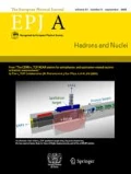
In this section, we summarize all expressions of the nuclear currents up to order Q in chiral expansion. Q denotes momenta and masses which are much smaller than the chiral symmetry breaking scale. We skip here the discussion of their construction. As an example, we discuss here Feynman diagrams which contribute to the two-nucleon vector current at leading order $Q^{-1}$. All other details about Feynman diagrams and specification of unitary phases can be found in [23, 142, 143, 166, 171].

5.1 Power counting

To organize chiral EFT calculations of nuclear current operators we follow Weinberg’s analysis [45, 46]. A Feynman diagram contributing to the current operator counts as $Q^\nu$. To derive the expression for the chiral dimension $\nu$, we consider a generic Feynman diagram which is proportional to the integral written symbolically as⁴

$$\begin{aligned} \delta ^{(4)}(p)^{C}\int (d^4q)^L\frac{1}{(q^2)^{I_p}} \frac{1}{q_0^{I_n}}\prod _i(q^{d_i})^{V_i}, \end{aligned}$$

(58)

where L is the number of loops, $I_p$ and $I_n$ are number of internal pion and nucleon lines, respectively. $d_i$ is the number of derivatives or pion mass insertions in the vertex $``i''$, $V_i$ denotes how many times the vertex $``i''$ appears in a given diagram, and C denotes the number of connected pieces in the diagram. From Eq. (58) we read off the index $\nu$:2019

$$\begin{aligned} \nu= & {} 4-4 C+4 L-2 I_p - I_n+\sum _{i} V_i d_i. \end{aligned}$$

(59)

The couplings of external sources are not taken into account in Eq. (59). We treat them as small but count them separately. They are also not taken into account in $d_i$. For example, $d_i=0$ for the leading-order photon-nucleon coupling. Using the identities

$$\begin{aligned} \sum _{i} V_i n_i= & {} 2 I_n + E_n \end{aligned}$$

(60)

$$\begin{aligned} \sum _{i} V_i p_i= & {} 2 I_p + E_p, \end{aligned}$$

(61)

where $n_i$ and $p_i$ denotes the number of nucleon and pion fields in the vertex “i”, respectively. $E_n$ and $E_p$ denote the number of external nucleon and pion lines, respectively. A well known topological identity which connects the number of loops with the number of internal lines is given by

$$\begin{aligned} L= & {} C + I_p + I_n - \sum _i V_i. \end{aligned}$$

(62)

Using Eqs. (60), (61) and (62) we get

$$\begin{aligned} \nu= & {} 4 - \frac{3}{2} E_n - E_p + \sum _i V_i \tilde{\kappa }_i, \end{aligned}$$

(63)

where $\tilde{\kappa }_i$ is given by

$$\begin{aligned} \tilde{\kappa }_i= d_i + \frac{3}{2} n_i + p_i - 4. \end{aligned}$$

(64)

We are not interested here in the pion production, so the number of external pions $E_p=0$. The number of nucleons is always conserved and we denote it by

$$\begin{aligned} N= & {} 2 E_n. \end{aligned}$$

(65)

The expression for the chiral dimension is then given by

$$\begin{aligned} \nu= & {} 4 - 3 N + \sum _i V_i \tilde{\kappa }_i. \end{aligned}$$

(66)

As was pointed out in [68], Eq. (66) is inconvenient since it depends on the total number of nucleons N. For example, one-pion exchange diagram in the two-nucleon system has the chiral order $\nu =0$ since $N=2$, $\tilde{\kappa }_1=1$ and $V_1=2$. In the presence of a third nucleon which acts as a spectator, it has chiral order $\nu =-3$ according to Eq. (66) since $N=3$. The origin of this discrepancy lies in the different normalization of two- and three-nucleon states:

$$\begin{aligned}&2N:\,\,\langle \mathbf {p}_1 \,\mathbf {p}_2|\mathbf {p}_1^\prime \, \mathbf {p}_2^\prime \rangle \,=\,\delta ^{(3)}(\mathbf {p}_1^\prime - \mathbf {p}_1) \delta ^{(3)}(\mathbf {p}_2^\prime - \mathbf {p}_2),\nonumber \\&3N:\,\,\langle \mathbf {p}_1 \,\mathbf {p}_2 \,\mathbf {p}_3|\mathbf {p}_1^\prime \, \mathbf {p}_2^\prime \,\mathbf {p}_3^\prime \rangle \nonumber \\&\quad =\delta ^{(3)}(\mathbf {p}_1^\prime - \mathbf {p}_1) \delta ^{(3)}(\mathbf {p}_2^\prime - \mathbf {p}_2) \delta ^{(3)}(\mathbf {p}_3^\prime - \mathbf {p}_3). \end{aligned}$$

(67)

One can circumvent this if one assigns a chiral dimension to the transition operator rather than to its matrix element in N-nucleon system. In this case, we have to modify the expression for $\nu$ by adding 3N to Eq. (66), accounting in this way for the normalization of the N-nucleon system. The expression for $\nu$ becomes independent of N but gives $\nu =6$ for one-pion-exchange. As was proposed in [68], we adjust the final expression for $\nu$ by subtracting from it 6 to get $\nu =0$ for one-pion-exchange, which is a convention. The final expression for the chiral dimension of the transition operator becomes

$$\begin{aligned} \nu= & {} -2 + \sum _i V_i \tilde{\kappa }_i. \end{aligned}$$

(68)

Similar to [149], we can also express the chiral dimension $\nu$ in terms of the inverse mass dimension of the coupling constant at a vertex “i”

$$\begin{aligned} \kappa _i= & {} d_i + \frac{3}{2} n_i + p_i + s_i - 4, \end{aligned}$$

(69)

where $s_i$ is the number of external sources which for the current operators can be only 0 or 1. Consistent with [149], we get

$$\begin{aligned} \nu= & {} -3 + \sum _i V_i \kappa _i. \end{aligned}$$

(70)

for the current operator and

$$\begin{aligned} \nu= & {} -2 + \sum _i V_i \kappa _i. \end{aligned}$$

(71)

for the nuclear force.

For the counting of the nucleon mass m, we adopt a two-nucleon power counting where 1/m-contributions count as two powers of Q [46]

$$\begin{aligned} \frac{Q}{m}\sim \frac{Q^2}{\varLambda _\chi ^2}. \end{aligned}$$

(72)

Here $\varLambda _\chi \sim 700\,\mathrm{MeV}$ and m are the chiral symmetry breaking scale and the nucleon mass, respectively.

5.2 Vector current up to order Q

5.2.1 Single-nucleon current

We start our discussion with electromagnetic vector current. Leading contribution to the vector current starts at the order $Q^{-3}$. At this order there is only a contribution to the single-nucleon charge operator. It is well known that chiral expansion of the single-nucleon currents does not converge well [5, 176, 177]. For moderate virtualities $Q^2\sim 0.3\,\mathrm{GeV}^2$, an explicit inclusion of $\rho$-meson is essential. For this reason the usual practice is to parametrize single-nucleon vector current by e.g. Sachs form factors and use their phenomenological form extracted from experimental data in practical calculations [199,200,201,202,203]. The general form of the single-nucleon current can be characterized by its non-relativistic one-over-nucleon-mass expansion given symbolically by

$$\begin{aligned} { V}_{\mathrm{1N}}^0= & {} { V}_{\mathrm{1N:static}}^0 + { V}_{\mathrm{1N:}1/m}^0 + { V}_{\mathrm{1N:}1/m^2}^0,\nonumber \\ \mathbf {{\varvec{V}}}_{\mathrm{1N}}= & {} \mathbf {{\varvec{V}}}_{\mathrm{1N:static}} + \mathbf {{\varvec{V}}}_{\mathrm{1N:}1/m} + \mathbf {{\varvec{V}}}_{\mathrm{1N:}1/m^2} +\mathbf {\varvec{V}}_{\mathrm{1N:off-shell}}.\nonumber \\ \end{aligned}$$

(73)

In terms of Sachs form factors, the non-relativistic charge is parametrized by

$$\begin{aligned} {V}_{\mathrm{1N:static}}^0= & {} e { G}_E(Q^2),\nonumber \\ { V}_{\mathrm{1N:} 1/m}^0= & {} \frac{i\,e}{2m^2}\mathbf {k}\cdot (\mathbf {k}_1\times \mathbf {\sigma }) {G}_M(Q^2),\nonumber \\ { V}_{\mathrm{1N:}1/m^2}^0= & {} -\frac{e}{8 m^2}\big [Q^2+2\,i\,\mathbf {k}\cdot (\mathbf {k}_1\times \mathbf {\sigma }) \big ] { G}_E(Q^2), \end{aligned}$$

(74)

and the non-relativistic current is given by

$$\begin{aligned} \mathbf {{\varvec{V}}}_{\mathrm{1N:static}}= & {} - \frac{i\,e}{2 m}\mathbf {k}\times \mathbf {\sigma }\, { G}_M(Q^2),\nonumber \\ \mathbf {{\varvec{V}}}_{\mathrm{1N:} 1/m}= & {} \frac{e}{m}\mathbf {k}_1\,{ G}_E(Q^2),\nonumber \\ \mathbf {{\varvec{V}}}_{\mathrm{1N:} 1/m^2}= & {} \frac{e}{16 m^3}\bigg [i\,\mathbf {k}\times \mathbf {\sigma }(2\mathbf {k}_1^{\,2}+Q^2)+2\,i\,\mathbf {k}\times \mathbf {k}_1\,\mathbf {k}_1\cdot \mathbf {\sigma }\nonumber \\&+ 2 \mathbf {k}_1(i\,\mathbf {k}\cdot (\mathbf {k}_1\times \mathbf {\sigma })+Q^2) -2\,\mathbf {k}\,\mathbf {k}\cdot \mathbf {k}_1\nonumber \\&+ 6\,i\,\mathbf {k}_1\times \mathbf {\sigma }\,\mathbf {k}\cdot \mathbf {k}_1\bigg ]{ G}_M(Q^2), \end{aligned}$$

(75)

where $\mathbf {k}$ is a photon momentum, $\mathbf {k}_1=(\mathbf {p}^{\,\prime }+\mathbf {p})/2$, and $\mathbf {p}^\prime ( \mathbf {p})$ are outgoing (incoming) momenta of the single–nucleon current operator. Virtuality in our kinematics is given by $Q^2=\mathbf {k}^2$. Note, that the form factors $G_E(Q^2)$ and $G_M(Q^2)$ in Eqs. (74) and (75) are operators in isospin space. The proton and neutron electromagnetic form factors can be extracted out of them by projecting these to the corresponding state.

As already briefly explained in Sect. 3 (see [149] for more comprehensive discussion) we apply unitary transformations on the Hamilton operator which explicitly depends on an external source and thus on time. These unitary transformations generate off-shell contributions to the longitudinal component of the current which depend on energy transfer $k_0$ and additional relativistic 1/m corrections. This contribution can also be parametrized by Sachs form factors via

$$\begin{aligned} \mathbf {\varvec{V}}_{\mathrm{1N:off-shell}}= & {} \mathbf {k}\bigg (k_0-\frac{\mathbf {k}\cdot \mathbf {k}_1}{m}\bigg ) \frac{e}{Q^2}\bigg [\big ({ G}_E(Q^2)-{ G}_E(0)\big )\nonumber \\&+\frac{i}{2m^2}\mathbf {k}\cdot (\mathbf {k}_1\times \mathbf {\sigma })\big ({ G}_M(Q^2)-{ G}_M(0)\big )\bigg ].\nonumber \\ \end{aligned}$$

(76)

5.2.2 Two-nucleon vector current

We switch now to a discussion of the two-nucleon vector current operator. Various contributions can be characterized by the number of pion exchanges and/or short-range interactions

$$\begin{aligned} V_{\mathrm{2N}}^\mu= & {} V_{\mathrm{2N:1\pi }}^\mu +V_{\mathrm{2N:2\pi }}^\mu +V_{\mathrm{cont}}^\mu . \end{aligned}$$

(77)

One-pion-exchange vector current Leading contribution to the one-pion-exchange (OPE) current shows up at the order $Q^{-1}$. The corresponding Feynman diagrams are listed in Fig. 1.

Fig. 1

Feynman diagrams which contribute to the two-nucleon vector current operator at order $Q^{-1}$

At this order we get a well known result for current operator

$$\begin{aligned} {\varvec{V}}_{\mathrm{2N:1\pi }}^{ (Q^{-1})}= & {} i \frac{e g_A^2}{4 F_\pi ^2} [{\varvec{\tau }}_1\times {\varvec{\tau }}_2]^3\frac{\mathbf {q}_2\cdot \mathbf {\sigma }_2}{q_2^2+M_\pi ^2} \nonumber \\&\bigg (\mathbf {q}_1\frac{\mathbf {q}_1\cdot \mathbf {\sigma }_1}{q_1^2+M_\pi ^2}-\mathbf {\sigma }_1\bigg )+ 1\leftrightarrow 2, \end{aligned}$$

(78)

and for the charge operator

$$\begin{aligned} { V}_{\mathrm{2N:1\pi }}^{0, (Q^{-1})}= & {} 0. \end{aligned}$$

(79)

Here e is electric coupling, $g_A$ axial vector coupling to the nucleon, $F_\pi$ pion decay constant, $M_\pi$ pion mass, $\mathbf {\sigma }_i$ and $\mathbf {\tau }_i$ are Pauli spin and isospin matrices with label $i=1,2$ labeling a corresponding nucleon. Momenta $\mathbf {q}_{1,2}$ are defined by

$$\begin{aligned} \mathbf {q}_i=\mathbf {p}_i^\prime - \mathbf {p}_i, \end{aligned}$$

(80)

where $i=1,2$ and $\mathbf {p}_i^\prime$ or $\mathbf {p}_i$ are outgoing or incoming momenta of the i-th nucleon, respectively.

There is no contribution at order $Q^0$ such that the next correction starts at the order Q which are leading one-loop contributions in the static limit and/or leading relativistic correction to OPE current

$$\begin{aligned} {V}_{\mathrm{2N:1\pi }}^{\mu , (Q)}= & {} {V}_{\mathrm{2N:1\pi , }\,\mathrm{static}}^{\mu , (Q)}+{V}_{\mathrm{2N: 1\pi , }1/m}^{\mu , (Q)}. \end{aligned}$$

(81)

The corresponding set of diagrams can be found in [143]. The explicit form of static contributions can be given in terms of scalar functions $f_{1\dots 6}(k)$. The vector contribution is given by [143]

$$\begin{aligned} \mathbf {V}_{\mathrm{2N:1\pi ,}\,\mathrm{static}}^{(Q)}= & {} \frac{\mathbf {\sigma }_2\cdot \mathbf {q}_2}{q_2^2+M_\pi ^2}\mathbf {q}_1 \times \mathbf {q}_2 \left[ [{\varvec{\tau }}_2]^3 \, f_1(k )\right. \nonumber \\&+ \left. \mathbf {\tau }_1 \cdot \mathbf {\tau }_2\, f_2(k ) \right] + \left[ \mathbf {\tau }_1\times \mathbf {\tau }_2 \right] ^3 \frac{\mathbf {\sigma }_2\cdot \mathbf {q}_2}{q_2^2 + M_\pi ^2} \nonumber \\&\times \biggl \{\mathbf {k}\left[ \mathbf {q}_2\times \mathbf {\sigma }_1 \right] f_3(k ) + \, \mathbf {k}\times \left[ \mathbf {q}_1\times \mathbf {\sigma }_1 \right] f_4(k)\nonumber \\&+ \mathbf {\sigma }_1 \cdot \mathbf {q}_1\, \left( \frac{\mathbf {k}}{k^2} - \frac{\mathbf {q}_1 }{q_1^2+M_\pi ^2} \right) f_5(k) \nonumber \\&+ \,\biggl [\frac{\mathbf {\sigma }_1\cdot \mathbf {q}_1}{q_1^2+M_\pi ^2}\mathbf {q}_1 - \mathbf {\sigma }_1 \biggr ]f_6(k )\biggl \} + 1\leftrightarrow 2,\nonumber \\ \end{aligned}$$

(82)

where the scalar functions $f_i(k)$ are given by

$$\begin{aligned} f_1\left( k \right)= & {} 2i e\frac{g_A}{F_\pi ^2}\, \bar{d}_8, \quad f_2\left( k \right) \,=\, 2i e\frac{g_A}{F_\pi ^2}\, \bar{d}_9 , \nonumber \\ f_3\left( k \right)= & {} - ie\frac{g_A}{64 F_\pi ^4\pi ^2} \left[ \,g_A^3\,\left( 2L(k)-1\right) + 32 F_\pi ^2\pi ^2 \bar{d}_{21} \right] \, , \nonumber \\ f_4\left( k \right)= & {} - ie\frac{g_A}{4 F_\pi ^2} \,\bar{d}_{22}, \nonumber \\ f_5\left( k \right)= & {} - ie \frac{g_A^2}{384 F_\pi ^4\pi ^2}\left[ 2(4M_\pi ^2 + k^2)L(k)\right. \nonumber \\&- \left. +\left( 6 \, \bar{l}_6 -\frac{5}{3}\right) k^2 8M_\pi ^2 \right] , \nonumber \\ f_6\left( k \right)= & {} - ie\frac{g_A}{ F_\pi ^2} M_\pi ^2 \,\bar{d}_{18}. \end{aligned}$$

(83)

Here $\bar{d}_i$ are low-energy constants (LEC) from the order $Q^3$ pion-nucleon Lagrangian [183]. $\bar{l}_6$ is a LEC from $Q^4$ pion-Lagrangian [37]. Their values can be fixed from pion-nucleon scattering and pion-photo- or electroproduction. The charge contribution is given by

$$\begin{aligned} V_{\mathrm{2N:1\pi ,}\,\mathrm{static}}^{0, (Q)}= & {} \frac{\mathbf {\sigma }_2\cdot \mathbf {q}_2}{q_2^2 + M_\pi ^2}[{\varvec{\tau }}_2]^3\biggr [ \mathbf {\sigma }_1\cdot \mathbf {k} \, \mathbf {q}_2 \cdot \mathbf {k} f_7( k ) \nonumber \\&+ \mathbf {\sigma }_1\cdot \mathbf {q}_2 f_8( k )\biggl ] + 1\leftrightarrow 2, \end{aligned}$$

(84)

where

$$\begin{aligned} f_7( k )= & {} e \frac{g_A^4}{64F_\pi ^4\pi } \left[ A(k) + \frac{M_\pi -4M_\pi ^2 \,A(k)}{k^2} \right] , \nonumber \\ f_8( k )= & {} e \frac{g_A^4}{64F_\pi ^4\pi } \left[ (4M_\pi ^2+k^2)A(k) - M_\pi \right] . \end{aligned}$$

(85)

The loop function L(k) and A(k) are defined

$$\begin{aligned} L(k)= & {} \frac{1}{2}\frac{\sqrt{k^2 + 4M_\pi ^2}}{k}\log \left( \frac{\sqrt{k^2 + 4M_\pi ^2}+k}{\sqrt{k^2 + 4M_\pi ^2}-k} \right) , \nonumber \\ A(k)= & {} \frac{1}{2k}\arctan \left( \frac{k}{2M_\pi }\right) . \end{aligned}$$

(86)

Relativistic corrections for the vector operator vanish

$$\begin{aligned} {\mathbf {V}}_{\mathrm{1\pi :}1/m}^{ (Q)}=0. \end{aligned}$$

(87)

Relativistic corrections for the charge operator are

$$\begin{aligned}&{V}_{\mathrm{2N: 1\pi , }1/m}^{0, (Q)}=\frac{e g_A^2}{16F_\pi ^2m} \frac{1}{q_2^2 + M_\pi ^2} \biggl \{(1-2\bar{\beta }_9) \nonumber \\&\quad \times \left( [{\varvec{\tau }}]_2^3 + \mathbf {\tau }_1\cdot \mathbf {\tau }_2 \right) \mathbf {\sigma }_1\cdot \mathbf {k} \mathbf {\sigma }_2\cdot \mathbf {q}_2 - i(1+2\bar{\beta }_9) \left[ \mathbf {\tau }_1\times \mathbf {\tau }_2\right] ^3\nonumber \\&\quad \times \biggl [ \mathbf {\sigma }_1\cdot \mathbf {k}_1 \mathbf {\sigma }_2\cdot \mathbf {q}_2 - \mathbf {\sigma }_2\cdot \mathbf {k}_2 \mathbf {\sigma }_1\cdot \mathbf {q}_2 - 2\, \frac{\mathbf {\sigma }_1\cdot \mathbf {q}_1}{q_1^2+M_\pi ^2}\mathbf {\sigma }_2\cdot \mathbf {q}_2\nonumber \\&\quad \times \mathbf {q}_1\cdot \mathbf {k}_1 \biggr ]\biggr \} + \frac{e g_A^2\, }{16 F_\pi ^2 m } \frac{ \mathbf {\sigma }_1\cdot \mathbf {q}_2 \, \mathbf {\sigma }_2\cdot \mathbf {q}_2 }{(q_2^2+M_\pi ^2)^2} \biggl [(2\bar{\beta }_8-1)\nonumber \\&\quad \times ([{\varvec{\tau }}_2]^3 + \mathbf {\tau _1}\cdot \mathbf {\tau }_2) \mathbf {q}_2\cdot \mathbf {k} + i \left[ \mathbf {\tau }_1 \times \mathbf {\tau }_2\right] ^3 \left( \left( 2\bar{\beta }_8 - 1\right) \mathbf {q}_2 \cdot \mathbf {k}_1\right. \nonumber \\&\quad - \left. \left( 2\bar{\beta }_8 + 1\right) \mathbf {q}_2\cdot \mathbf {k}_2\,\right) \biggr ] + 1\leftrightarrow 2. \end{aligned}$$

(88)

Here $\bar{\beta }_8$ and $\bar{\beta }_9$ are phases from unitary transformations which are not fixed. The same phases show up in nuclear forces. Usually they are fixed by requirement of minimal non-locality of the OPE NN potential.

Two-pion-exchange vector current Contributions to two-pion-exchange (TPE) vector current start to show up at order Q. They are parameter-free. The corresponding diagrams can be found in [142]. Due to the coupling of the vector source to two pions there appear loop functions which depend on three momenta $\mathbf {k}, \mathbf {q_1}$ and $\mathbf {q}_2$ which are momentum transfer of the vector source, momentum transfer of the first and second nucleons, respectively. This leads to a somewhat lengthy expression which have been derived in [142] and are listed in Appendix D for completeness:

Short-range vector current The first contribution to short-range two-nucleon current shows up at the order Q. The diagrams with short-range interactions at this order can be found in [143]. There are two contributions [143]

$$\begin{aligned} V_{\mathrm{2N:\,cont}}^{\mu , (Q)}= & {} V_{\mathrm{2N: cont, tree}}^{\mu , (Q)} + V_{\mathrm{2N: cont, loop}}^{\mu , (Q)}. \end{aligned}$$

(89)

The current contribution coming from tree-diagrams is given by

$$\begin{aligned}&{\mathbf {V}}_{\mathrm{2N: cont, tree}}^{(Q)}\, = \, e\,\frac{i}{16}\left[ \mathbf {\tau }_1 \times \mathbf {\tau }_2\right] ^3 \,\biggl [\left( C_2 +3C_4 + C_7\right) \, \mathbf {q}_1 \nonumber \\&\quad - \left( -C_2 + C_4 + C_7 \right) \, \, \left( \mathbf {\sigma }_1 \cdot \mathbf {\sigma }_2 \right) \, \, \mathbf {q}_1 + C_7 \, \left( \mathbf {\sigma }_2\cdot \mathbf {q}_1 \, \mathbf {\sigma }_1\right. \nonumber \\&\quad +\left. \mathbf {\sigma }_1\cdot \mathbf {q}_1 \, \mathbf {\sigma }_2 \right) \biggr ] - e\,\frac{C_5 \, i}{16}\, [{\varvec{\tau }}_1]^3 \, \left[ \left( \mathbf {\sigma }_1 + \mathbf {\sigma }_2 \right) \times \mathbf {q}_1 \right] \nonumber \\&\quad + i e L_1 \, [{\varvec{\tau }}_1]^3 \, \left[ \left( \mathbf {\sigma }_1 - \mathbf {\sigma }_2 \right) \times \mathbf {k}\right] \nonumber \\&\quad + i e L_2 \, \left[ \left( \mathbf {\sigma }_1 + \mathbf {\sigma }_2 \right) \times \mathbf {q}_1 \right] \, . \end{aligned}$$

(90)

As can be seen from Eq. (90) there are $C_i$ LECs which also contribute to the two-nucleon potential and appear here due to the minimal coupling, and there are two additional constants $L_{1,2}$ which describe entirely electromagnetic effects. Charge short-range contribution from tree diagrams at order Q vanishes

$$\begin{aligned} {V}_{\mathrm{2N: cont, tree}}^{0, (Q)}= & {} 0. \end{aligned}$$

(91)

There are also contributions from one-loop diagrams which include one leading-order two-nucleon contact interaction and two-pion propagators. They only contribute to charge operator⁵

$$\begin{aligned} {V}_{\mathrm{2N: cont, loop}}^{0, (Q)}= & {} C_T\, [{\varvec{\tau }}_1]^3\, \left[ \mathbf {\sigma }_1\cdot \mathbf {k}\,\mathbf {\sigma }_2\cdot \mathbf {k}\, f_{9}(k ) \right. \nonumber \\&+\left. \mathbf {\sigma }_1\cdot \mathbf {\sigma }_2 \, f_{10}( k )\right] , \end{aligned}$$

(92)

where

$$\begin{aligned} f_{9}( k )= & {} e \frac{g_A^2}{16F_\pi ^2\pi } \left( A(k) + \frac{M_\pi -4M_\pi ^2 \,A(k)}{k^2} \right) , \nonumber \\ f_{10}( k )= & {} e\frac{g_A^2}{16 F_\pi ^2\pi }\, \left( M_\pi -(4M_\pi ^2 + 3k^2)\,A(k) \right) . \end{aligned}$$

(93)

Corresponding contributions to the current operator vanish

$$\begin{aligned} {\mathbf {V}}_{\mathrm{cont: loop}}^{ (Q)}= & {} 0. \end{aligned}$$

(94)

5.2.3 Three-nucleon vector current

At the order Q there are first contributions to three-nucleon vector current [149]. There are no contributions to the vector operator

$$\begin{aligned} {\mathbf {V}}_{\mathrm{3N}}^{(Q)}= & {} 0. \end{aligned}$$

(95)

Contributions to the charge operator can be parametrized in the form

$$\begin{aligned} {V}_{\mathrm{3N}}^{0, (Q)}= & {} \bigg [\frac{(\mathbf {q}_1+\mathbf {q}_2)\cdot \mathbf {\sigma }_3}{(\mathbf {q}_1+\mathbf {q}_2)^2+M_\pi ^2}+ \frac{\mathbf {q}_3\cdot \mathbf {\sigma }_3}{q_3^2+M_\pi ^2}\bigg ]\nonumber \\&\times \big ({v}_{\mathrm{3N: long}}+{v}_{\mathrm{3N: short}}\big ) + 5\,\mathrm{permutations}. \end{aligned}$$

(96)

where the long- and short-range contributions are given by

$$\begin{aligned} {v}_{\mathrm{3N: long}}= & {} \frac{e}{16 F_\pi ^4} \frac{\mathbf {q}_1\cdot \mathbf {\sigma }_1}{q_1^2+M_\pi ^2}\bigg [\big ({\varvec{\tau }}_1\cdot {\varvec{\tau }}_3 [{\varvec{\tau }}_2]^3 -{\varvec{\tau }}_2\cdot {\varvec{\tau }}_3 [{\varvec{\tau }}_1]^3\big )\nonumber \\&\times \bigg (-2 g_A^4\frac{q_1^2+\mathbf {q}_1\cdot \mathbf {q}_2}{(\mathbf {q}_1+\mathbf {q}_2)^2+M_\pi ^2} + g_A^2\bigg ) \nonumber \\&- i[{\varvec{\tau }}_1\times {\varvec{\tau }}_3]^3 2 g_A^4\frac{q_1^2+\mathbf {q}_1\cdot \mathbf {q}_2}{(\mathbf {q}_1+\mathbf {q}_2)^2 +M_\pi ^2}\bigg ],\end{aligned}$$

(97)

$$\begin{aligned} {v}_{\mathrm{3N: short}}= & {} -[{\varvec{\tau }}_1\times {\varvec{\tau }}_3]^3 \frac{e\,g_A^2 C_T}{2 F_\pi ^2} \frac{(\mathbf {q}_1+\mathbf {q}_2)\cdot (\mathbf {\sigma }_1\times \mathbf {\sigma }_2) }{(\mathbf {q}_1+\mathbf {q}_2)^2+M_\pi ^2}.\nonumber \\ \end{aligned}$$

(98)

Due to the approximate spin-isospin $\mathrm{SU}(4)$ Wigner symmetry [150], $C_T$ appears to be small such that we do not expect large contributions from short-range part of the three-nucleon vector current.

5.3 Axial vector current up to order Q

The weak sector of nuclear physics can be probed by a nuclear axial-vector current. We give here its expressions up to order Q in chiral expansion.

5.3.1 Single-nucleon axial vector current

The leading-order contribution to an axial vector current shows up at order $Q^{-3}$ where axial-vector source couples directly to a single-nucleon or to a pion, which itself propagates and couples to a single-nucleon generating in this way a pion-pole term. It is convenient to parametrize the single-nucleon current by the axial and pseudoscalar form factors. Up to the order Q the parametrization is given by

$$\begin{aligned} A_{\mathrm{1N}}^{\mu , a}= & {} A_{\mathrm{1N:on-shell}}^{\mu , a}+A_{\mathrm{1N:off-shell}}^{\mu , a}. \end{aligned}$$

(99)

The charge operator is parametrized by

$$\begin{aligned} {A}_{\mathrm{1N:on-shell}}^{0, a}= & {} \frac{[{\varvec{\tau }}]^a}{2} \bigg [-\frac{\mathbf {k}_1\cdot \mathbf {\sigma }}{m} {G}_A(t) + \frac{\mathbf {k}\cdot \mathbf {k}_1}{m}\bigg (\frac{\mathbf {k}\cdot \mathbf {\sigma }}{4 m^2} \nonumber \\&- \frac{\mathbf {k}\cdot \mathbf {\sigma }(k^2+4 k_1^2)+4 \mathbf {k}\cdot \mathbf {k}_1 \mathbf {k}_1\cdot \mathbf {\sigma }}{32 m^4}\bigg )\nonumber \\&\times G_P(t)\bigg ],\nonumber \\ {A}_{\mathrm{1N:off-shell}}^{0, a}= & {} 0. \end{aligned}$$

(100)

The current operator is parametrized by

$$\begin{aligned} \mathbf {{A}}_{\mathrm{1N:on-shell}}^{a}= & {} \frac{[{\varvec{\tau }}]^a}{2}\bigg [\bigg (-\mathbf {\sigma } + \frac{1}{8 m^2}\Big (4\,\mathbf {\sigma } \,k_1^2-4\, \mathbf {k}_1\, \mathbf {k}_1\cdot \mathbf {\sigma } \nonumber \\&+ 2\, i\,\mathbf {k}\times \mathbf {k}_1 + \mathbf {k}\,\mathbf {k}\cdot \mathbf {\sigma }\Big ) \bigg ) G_A(t) \nonumber \\&+\mathbf {k}\,\bigg (\frac{\mathbf {k}\cdot \mathbf {\sigma }}{4 m^2}-\frac{1}{32 m^4}\Big (\mathbf {k}\cdot \mathbf {\sigma }\, k^2 \nonumber \\&+ 4\,\mathbf {k}\cdot \mathbf {\sigma }\, k_1^2 + 4\, \mathbf {k}_1\cdot \mathbf {\sigma }\,\mathbf {k}\cdot \mathbf {k}_1\Big )\bigg )G_P(t)\bigg ],\nonumber \\ \mathbf {A}_{\mathrm{1N:off-shell}}^a= & {} \mathbf {k}\bigg (k_0-\frac{\mathbf {k}\cdot \mathbf {k}_1}{m}\bigg ) \frac{[{\varvec{\tau }}]^a}{16 m^3}\Big [- (1+2\beta _9)\nonumber \\&\times \,\mathbf {k}_1\cdot \mathbf {\sigma }\, G_P(t) + (1+2\beta _8) \mathbf {k}\cdot \mathbf {k}_1 \mathbf {k}\cdot \mathbf {\sigma }\,G_P^\prime (t)\Big ],\nonumber \\ \end{aligned}$$

(101)

Chiral EFT results are given by chiral expansion of the axial and pseudoscalar form factors. Corresponding expressions are worked out in [23]. To make this review self-consistent we will briefly discuss them here.

The well-known leading-order result for the axial charge and current operators have the form

$$\begin{aligned} A^{0, a \, (Q^{-3})}_{\mathrm{1N: \, static}}= & {} 0,\nonumber \\ \mathbf {A}^{ a \, (Q^{-3})}_{\mathrm{1N: static}}= & {} -\frac{g_A}{2}[{\varvec{\tau }}_i]^a\bigg (\mathbf {\sigma }_i - \frac{\mathbf {k}\, \mathbf {k}\cdot \mathbf {\sigma }_i}{k^2+M_\pi ^2}\bigg ). \end{aligned}$$

(102)

There are only vanishing contributions at order $Q^{-2}$. At order $Q^{-1}$, we encounter three kinds of corrections. First, there are terms emerging from the time-dependence of unitary transformations which have the form

$$\begin{aligned} A^{0, a \, (Q^{-1})}_{\mathrm{1N: UT^\prime }}= & {} \frac{g_A}{2} \frac{k_0}{k^2+M_\pi ^2}\mathbf {k}\cdot \mathbf {\sigma }_i [{\varvec{\tau }}_i]^a,\end{aligned}$$

(103)

$$\begin{aligned} \mathbf {A}^{ a \, (Q^{-1})}_{\mathrm{1N: UT^\prime }}= & {} 0. \end{aligned}$$

(104)

and contribute to ${A}_{\mathrm{1N:off-shell}}^{\mu , a}$. Secondly, at order $Q^{-1}$ there are static limit contributions to $A_{\mathrm{1N:on-shell}}^{\mu , a}$ which are given by

$$\begin{aligned} A^{0, a \, (Q^{-1})}_{\mathrm{1N: static}}= & {} 0,\nonumber \\ \mathbf {A}^{a \, (Q^{-1})}_{\mathrm{1N: static}}= & {} \frac{1}{2}\bar{d}_{22}\Big (\mathbf {\sigma }_i k^2-\mathbf {k}\, \mathbf {k}\cdot \mathbf {\sigma }_i\Big )[{\varvec{\tau }}_i]^a \nonumber \\&- \bar{d}_{18} M_\pi ^2[{\varvec{\tau }}_i]^a \frac{\mathbf {k}\,\mathbf {k}\cdot \mathbf {\sigma }_i}{k^2+M_\pi ^2}. \end{aligned}$$

(105)

Finally, there are leading relativistic 1/m-corrections which in our counting scheme start contributing at order $Q^{-1}$ to ${A}_{\mathrm{1N:on-shell}}^{\mu , a}$ and read

$$\begin{aligned} A^{0, a \, (Q^{-1})}_{\mathrm{1N:} 1/m}= & {} - \frac{g_A}{2 m } [{\varvec{\tau }}_i]^a \, \mathbf {\sigma }_i \cdot \mathbf {k}_i \,,\end{aligned}$$

(106)

$$\begin{aligned} \mathbf {A}^{ a \, (Q^{-1})}_{\mathrm{1N: 1/m}}= & {} 0, \end{aligned}$$

(107)

where

$$\begin{aligned} \mathbf {k}=\mathbf {p_i}^{\prime } - \mathbf {p}_i, \quad \mathbf {k}_i=\frac{\mathbf {p_i}^{\prime } + \mathbf {p}_i}{2}. \end{aligned}$$

(108)

There are no corrections to the 1N charge and current operators at the order $Q^0$. Finally, there are various contributions at order Q. The off-shell contributions coming from time-dependent unitary transformations give different contributions. One of them is coming from relativistic corrections which are proportional to $k_0/m$ and are given by

$$\begin{aligned} A^{0, a \, (Q)}_{\mathrm{1N: }1/m, \mathrm{UT^\prime }}= & {} 0,\nonumber \\ \mathbf {A}^{ a \, (Q)}_{\mathrm{1N: }1/m, \mathrm{UT^\prime }}= & {} -\frac{g_A k_0}{8 m}\frac{\mathbf {k}}{k^2+M_\pi ^2}[{\varvec{\tau }}_i]^a \bigg (2(1 + 2 \,\bar{\beta }_9)\mathbf {\sigma }_i \cdot \mathbf {k}_i \nonumber \\&- (1 + 2 \,\bar{\beta }_8)\mathbf {k}\cdot \mathbf {\sigma }_i\frac{p_i^{\prime \,2}-p_i^2}{k^2+M_\pi ^2}\bigg ). \end{aligned}$$

(109)

They explicitly depend on unitary phases $\bar{\beta }_8$ and $\bar{\beta }_9$. Note that these are the same unitary phases that influence a non-locality degree of relativistic $1/m^2$ corrections of the one-pion-exchange nuclear force. For the static part which is proportional to $k_0$, we get nonvanishing contributions

$$\begin{aligned} A^{0, a \, (Q)}_{\mathrm{1N: static, UT^\prime }}= & {} -k_0 \frac{[{\varvec{\tau }}_i]^a}{2} \mathbf {k}\cdot \mathbf {\sigma }_i \bigg [\bar{d}_{22}+ \frac{2 \bar{d}_{18} M_\pi ^2}{k^2+M_\pi ^2}\bigg ]\,,\nonumber \\ \mathbf {A}^{ a \, (Q)}_{\mathrm{1N: static, UT^\prime }}= & {} 0. \end{aligned}$$

(110)

The second class of order-Q contributions involves relativistic $1/m^2$-corrections:

$$\begin{aligned} A^{0, a \, (Q)}_{\mathrm{1N:} \, 1/m^2}= & {} 0,\nonumber \\ \mathbf {A}^{ a \, (Q)}_{\mathrm{1N: 1/m^2}}= & {} \frac{g_A}{16 m^2}[{\varvec{\tau }}_i]^a\bigg (\mathbf {k}\,\mathbf {k}\cdot \mathbf {\sigma }_i(1-2\bar{\beta }_8)\frac{(p_i^{\prime \,2}-p_i^2)^2}{(k^2+M_\pi ^2)^2}\nonumber \\&-2 \mathbf {k} \frac{(p_i^{\prime \, 2} + p_i^2)\mathbf {k}\cdot \mathbf {\sigma }_i-2 \bar{\beta }_9 (p_i^{\prime \, 2} - p_i^2)\mathbf {k}_i\cdot \mathbf {\sigma }_i }{k^2+M_\pi ^2}\nonumber \\&+2\,i\,[\mathbf {k}\times \mathbf {k}_i]+\mathbf {k}\,\mathbf {k}\cdot \mathbf {\sigma }_i - 4\,\mathbf {k}_i\,\mathbf {k}_i\cdot \mathbf {\sigma }_i \nonumber \\&+ \mathbf {\sigma }_i\Big (2(p_i^{\prime \,2}+p_i^2)-k^2\Big )\bigg ). \end{aligned}$$

(111)

These are a linear combination of on-shell and off-shell contributions. The third kind of order-Q contributions emerges from relativistic 1/m-corrections to the leading one-loop terms which contributes to $A_{\mathrm{1N:on-shell}}^{\mu , a}$:

$$\begin{aligned} A^{0, a \, (Q)}_{\mathrm{1N:} \, 1/m}= & {} \bar{d}_{22}\mathbf {k}_i\cdot \mathbf {\sigma }_i[{\varvec{\tau }}_i]^a\frac{k^2}{2 m}, \end{aligned}$$

(112)

$$\begin{aligned} \mathbf {A}^{ a \, (Q)}_{\mathrm{1N: 1/m}}= & {} 0. \end{aligned}$$

(113)

Finally, static two-loop contributions to the on-shell current are given by

$$\begin{aligned} A^{0, a \, (Q)}_{\mathrm{1N: static}}= & {} 0,\nonumber \\ \mathbf {A}^{a \, (Q)}_{\mathrm{1N: \, static}}= & {} -\frac{1}{2}[{\varvec{\tau }}_i]^a\mathbf {\sigma }_i \Big ( - f_0^A M_\pi ^2 k^2 + f_1^A k^4 \nonumber \\&+ G_A^{(Q^4)}(-k^2)\Big )+\frac{1}{8}\mathbf {k}\,\mathbf {k}\cdot \mathbf {\sigma }_i [{\varvec{\tau }}_i]^a\Big ( -4 f_0^A M_\pi ^2 \nonumber \\&- f_1^P k^2 + G_P^{(Q^2)}(-k^2)\Big )\,.\quad \quad \end{aligned}$$

(114)

Here we perform the chiral expansion of the axial form factor which can be found e.g. in [151, 152], see also [153, 154] for results obtained within Lorentz-invariant formulations. Rewritten in our notation, the chiral expansion of the axial form factor is given by

$$\begin{aligned} G_A(t)= & {} g_A+(\bar{d}_{22}+f_0^A M_\pi ^2) t + f_1^A t^2 + G_A^{(Q^4)}(t) \nonumber \\&+ {\mathcal {O}}(Q^5), \end{aligned}$$

(115)

where $f_i^A$ are LECs of dimension $\mathrm{GeV}^{-4}$ and

$$\begin{aligned} G_A^{(Q^4)}(t) = \frac{t^3}{\pi }\int _{9 M_\pi ^2}^\infty \frac{\mathrm{Im}\,G_A^{(Q^4)}(t^\prime \,)}{t^{\prime \,3}(t^\prime - t - i \epsilon )}d t^\prime , \end{aligned}$$

(116)

with the imaginary part calculated utilizing the Cutkosky rules [151]

$$\begin{aligned} \mathrm{Im}\,G_A^{(Q^4)}(t)= & {} \frac{g_A}{192 \pi ^3 F_\pi ^4}\int _{z^2 < 1} d \omega _1 d \omega _2\bigg [6 g_A^2 (\sqrt{t}\, \omega _1 - M_\pi ^2)\nonumber \\&\times \Big (\frac{l_2}{l_1} + z\Big )\frac{\arccos (-z)}{\sqrt{1-z^2}}\nonumber \\&+2 g_A^2\Big (M_\pi ^2 - \sqrt{t}\,\omega _1 -\omega _1^2\Big ) + M_\pi ^2 - \sqrt{t}\,\omega _1\nonumber \\&+ 2\omega _1^2\bigg ], \end{aligned}$$

(117)

where

$$\begin{aligned} \omega _i= & {} \sqrt{l_i^2 + M_\pi ^2}\quad \mathrm{with}\quad i=1,2, \quad \mathrm{and}\nonumber \\ z= & {} \hat{l}_1\cdot \hat{l}_2=\frac{\omega _1 \omega _2-\sqrt{t}(\omega _1+\omega _2)+\frac{1}{2}(t+M_\pi ^2)}{l_1 l_2}. \end{aligned}$$

(118)

Here and in what follows, $l_i \equiv | \mathbf {l}_i |$, while $\hat{l}_i \equiv \mathbf {l}_i/l_i$. The pseudoscalar form-factor up to order $Q^4$ is given by [159]

$$\begin{aligned} G_P(t)= & {} \frac{4m g_{\pi N} F_\pi }{M_\pi ^2-t}-\frac{2}{3}g_A m^2 \langle r_A^2\rangle + m^2 f_1^P t\nonumber \\&+ m^2 G_P^{(Q^2)}(t)+ {\mathcal {O}}(Q^3), \end{aligned}$$

(119)

where $f_i^P$ denotes the corresponding linear combinations of the LECs of dimension $\mathrm{GeV}^{-4}$ from ${\mathcal L}_{\pi N}^{(5)}$ and

$$\begin{aligned} G_P^{(Q^2)}(t)= & {} \frac{t^2}{\pi }\int _{9 M_\pi ^2}^\infty \frac{\mathrm{Im}\,G_P^{(Q^2)}(t^\prime \,)}{t^{\prime \,2}(t^\prime - t - i \epsilon )}d t^\prime , \end{aligned}$$

(120)

with the imaginary part calculated using the Cutkosky rules [159]

$$\begin{aligned} \mathrm{Im}\,G_P^{(Q^2)}(t)= & {} \mathrm{Im}\,G_P^{(1)}(t) + \mathrm{Im}\,G_P^{(2)}(t) \end{aligned}$$

(121)

and

$$\begin{aligned} \mathrm{Im}\,G_P^{(1)}(t)= & {} \frac{g_A}{8\pi ^3 F_\pi ^4}\int _{z^2<1} d\omega _1 d\omega _2\bigg [\frac{1}{18}-\frac{M_\pi ^4}{12(t-M_\pi ^2)^2}\nonumber \\&+\frac{4\omega _1^2-M_\pi ^2}{6 t}+\frac{\omega _1^2(3 M_\pi ^2-t)}{(t-M_\pi ^2)^2}\nonumber \\&+\frac{2 M_\pi ^2 \omega _1 \omega _2 z}{t(t-M_\pi ^2)} \frac{l_2}{l_1}\bigg ],\nonumber \\ \mathrm{Im}\,G_P^{(2)}(t)= & {} \frac{g_A^3}{8\pi ^3 F_\pi ^4 t}\int _{z^2<1} d\omega _1 d\omega _2\bigg [(M_\pi ^2-\sqrt{t}\omega _1)\nonumber \\&\times \bigg (z+\frac{l_2}{l_1}\bigg )\frac{\arccos (-z)}{\sqrt{1-z^2}} + \frac{l_1^2}{3}+\frac{t}{9}\nonumber \\&+\frac{M_\pi ^2}{t-M_\pi ^2}\bigg (\frac{7}{8} \sqrt{t}-\omega _1-\omega _2\bigg )\bigg (2\omega _1 z \frac{l_2}{l_1}\nonumber \\&+\sqrt{t}+\Big ((t+M_\pi ^2)(4\omega _1-\sqrt{t}) -4\sqrt{t}\omega _1\omega _2\Big )\nonumber \\&\times \frac{\arccos (-z)}{2 l_1 l_2 \sqrt{1-z^2}}\bigg )\bigg ]. \end{aligned}$$

(122)

It is important to note that the induced pseudoscalar form factor is related to the induced pseudoscalar coupling constant

$$\begin{aligned} g_P= & {} \frac{M_\mu }{2 m} G_P(t = -0.88 M_\mu ^2), \end{aligned}$$

(123)

which is measured in muon capture experiment [155]. For theoretical determination of $g_P$ by using chiral Ward identities of QCD we refer to a groundbreaking work [156], see also [157, 158].

In practical calculations, alternatively to the chiral expansion of the axial and pseudoscalar form factors, one can take their empirical parametrization [157]. This is in particular reasonable if we would like to consider electroweak probes of nuclei without being affected by the convergence issue of the chiral expansion of electroweak single-nucleon currents.

5.3.2 Two-nucleon axial vector current

We now switch to a discussion of the two-nucleon axial vector current operator. Various contributions can be characterized by the number of pion exchanges and/or short-range interactions

$$\begin{aligned} A_{\mathrm{2N}}^{\mu ,a}= & {} A_{\mathrm{2N:\,}1\pi }^{\mu ,a}+A_{\mathrm{2N:\,}2\pi }^{\mu ,a}+A_{\mathrm{2N:\,}\mathrm{cont}}^{\mu ,a}. \end{aligned}$$

(124)

One-pion-exchange axial vector current Leading contribution to the one-pion-exchange (OPE) current shows up at the order $Q^{-1}$. At this order we get a well known result [137, 160, 161]

$$\begin{aligned} A_{\mathrm{2N:\,}1\pi }^{0, a \; ({Q^{-1}})}= & {} -\frac{i g_A \mathbf {q}_1\cdot \mathbf {\sigma }_1 [{\varvec{\tau }}_1\times {\varvec{\tau }}_2]^a}{4 F_\pi ^2 \left( q_1^2 +M_\pi ^2\right) }\; + 1 \leftrightarrow 2\,, \end{aligned}$$

(125)

$$\begin{aligned} \mathbf {A}_{\mathrm{2N:\,}1\pi }^{a \; ({Q^{-1}})}= & {} 0. \end{aligned}$$

(126)

At the order $Q^0$ there are only contributions to the vector operator

$$\begin{aligned}&\mathbf {A}_{\mathrm{2N:}\, 1\pi }^{a \; ({Q^{0}})} \,=\, \frac{g_A}{2 F_\pi ^2} \frac{\mathbf {\sigma }_1 \cdot \mathbf {q}_1}{q_1^2 + M_\pi ^2} \bigg \{ [{\varvec{\tau }}_1]^a \bigg [ - 4 c_1 M_\pi ^2 \frac{\mathbf {k}}{k^2 + M_\pi ^2}\nonumber \\&\quad + 2 c_3 \bigg ( \mathbf {q}_1 - \frac{\mathbf {k} \, \mathbf {k} \cdot \mathbf {q}_1}{k^2 + M_\pi ^2} \bigg ) \bigg ]+ c_4 [ \varvec{\tau }_1 \times \varvec{\tau }_2 ]^a \bigg ( \mathbf {q}_1 \times \mathbf {\sigma }_2 \nonumber \\&\quad - \frac{\mathbf {k} \, \mathbf {k} \cdot \mathbf {q}_1 \times \mathbf {\sigma }_2}{k^2 + M_\pi ^2} \bigg ) -\frac{\kappa _v}{4 m} [ \varvec{\tau }_1 \times \varvec{\tau }_2 ]^a \mathbf {k}\times \mathbf {\sigma }_2\bigg \} \nonumber \\&\quad + 1 \leftrightarrow 2, \end{aligned}$$

(127)

where $c_i$ denote the LECs from $\mathcal {L}_{\pi N}^{(2)}$ and $\kappa _v$ is the isovector anomalous magnetic moment of the nucleon.

At the order Q there are leading one-loop contributions in the static limit and/or leading relativistic correction to OPE current

$$\begin{aligned} {A}_{\mathrm{2N:1\pi }}^{\mu , a (Q)}= & {} {A}_{\mathrm{2N:1\pi ,}\,\mathrm{static}}^{\mu ,a (Q)}+{A}_{\mathrm{2N:1\pi , }1/m}^{\mu ,a (Q)}+{A}_{\mathrm{2N:1\pi , UT}^\prime }^{\mu ,a (Q)}. \end{aligned}$$

(128)

The explicit form of static contributions can be given in terms of scalar functions $h_{1\dots 8}(q_2)$. The vector contribution is given by

$$\begin{aligned}&\mathbf {A}_{\mathrm{2N:} 1\pi ,\mathrm{static}}^{a \, (Q)}= \frac{4 F_\pi ^2}{g_A} \frac{\mathbf {q}_1 \cdot \mathbf {\sigma }_1}{q_1^2 + M_\pi ^2} \Big \{ [ \varvec{\tau }_1 \times \varvec{\tau }_2 ]^a \nonumber \\&\quad \times \Big ( [\mathbf {q}_1 \times \mathbf {\sigma }_2 ] \, h_1(q_2) + [\mathbf {q}_2 \times \mathbf {\sigma }_2 ] \, h_2(q_2)\Big ) \nonumber \\&\quad + [{\varvec{\tau }}_1]^a \big (\mathbf {q}_1 - \mathbf {q}_2\big ) h_3(q_2) \Big \}+ \frac{4 F_\pi ^2}{g_A}\frac{\mathbf {q}_1 \cdot \mathbf {\sigma }_1 \,\mathbf {k} }{(k^2 + M_\pi ^2)(q_1^2 + M_\pi ^2)}\nonumber \\&\quad \times \Big \{[{\varvec{\tau }}_1]^a h_4(q_2) + [ \varvec{\tau }_1 \times \varvec{\tau }_2 ]^a \mathbf {q}_1 \cdot [\mathbf {q}_2 \times \mathbf {\sigma }_2] h_5(q_2)\Big \} \nonumber \\&\quad + \; 1 \leftrightarrow 2, \end{aligned}$$

(129)

and the charge contribution is given by

$$\begin{aligned}&A_{\mathrm{2N:} \, 1\pi ,\mathrm{static}}^{0, a \, (Q)}= i \frac{4 F_\pi ^2}{g_A} \frac{\mathbf {q}_1 \cdot \mathbf {\sigma }_1}{q_1^2 + M_\pi ^2} \Big \{ [ \varvec{\tau }_1 \times \varvec{\tau }_2 ]^a \, \big ( h_6(q_2)\nonumber \\&\quad + k^2 h_7(q_2) \big ) + [{\varvec{\tau }}_1]^a \, \mathbf {q}_1 \cdot [ \mathbf {q}_2 \times \mathbf {\sigma }_2 ] \,h_8(q_2) \Big \} + 1 \leftrightarrow 2,\nonumber \\ \end{aligned}$$

(130)

where the scalar functions $h_i (q_2)$ are given by

$$\begin{aligned} h_1(q_2)= & {} -\frac{g_A^6M_\pi }{128\pi F_\pi ^6}, \nonumber \\ h_2(q_2)= & {} \frac{g_A^4M_\pi }{256\pi F_\pi ^6} + \frac{g_A^4 A(q_2)\left( 4M_\pi ^2+q_2^2 \right) }{256\pi F_\pi ^6},\nonumber \\ h_3(q_2)= & {} \frac{g_A^4\left( g_A^2+1 \right) M_\pi }{128\pi F_\pi ^6} +\frac{g_A^4A(q_2)\left( 2M_\pi ^2+q_2^2 \right) }{128\pi F_\pi ^6}, \nonumber \\ h_4(q_2)= & {} \frac{g_A^4}{256\pi F_\pi ^6}\Big (A(q_2)\left( 2M_\pi ^4+5M_\pi ^2q_2^2+ 2 q_2^4\right) \nonumber \\&+\left( 4g_A^2+1\right) M_\pi ^3+2\left( g_A^2+1 \right) M_\pi q_2^2\Big ),\nonumber \\ h_5(q_2)= & {} -\frac{g_A^4}{256\pi F_\pi ^6}\Big (A(q_2)\left( 4M_\pi ^2+q_2^2\right) \nonumber \\&+ \left( 2g_A^2+1\right) M_\pi \Big ),\nonumber \\ h_6(q_2)= & {} \frac{g_A^2\left( 3\left( 64+128 g_A^2 \right) M_\pi ^2+8\left( 19 g_A^2+5\right) q_2^2\right) }{36864\pi ^2F_\pi ^6}\nonumber \\&-\frac{g_A^2}{768\pi ^2F_\pi ^6} L(q_2)\big (\left( 8g_A^2+4\right) M_\pi ^2\nonumber \\&+\left( 5g_A^2+1 \right) q_2^2\big )+\frac{\bar{d}_{18}g_A M_\pi ^2}{8 F_\pi ^4}-\frac{\bar{d}_{5}g_A^2M_\pi ^2}{2F_\pi ^4}\nonumber \\&-\frac{g_A^2(2\bar{d}_{2}+ \bar{d}_{6})\left( M_\pi ^2+q_2^2 \right) }{16F_\pi ^4},\nonumber \\ h_7(q_2)= & {} \frac{g_A^2(2\bar{d}_{2}-\bar{d}_{6})}{16F_\pi ^4},\nonumber \\ h_8(q_2)= & {} -\frac{g_A^2(\bar{d}_{15}-2\bar{d}_{23})}{8F_\pi ^4}. \end{aligned}$$

(131)

Here $\bar{d}_i$ are low-energy constants (LEC) from $Q^3$ pion-nucleon Lagrangian. Their values can be fixed from pion-nucleon scattering and axial-pion-production.

The relativistic corrections for the charge operator vanish

$$\begin{aligned} A_{\mathrm{2N:} \, 1\pi , \, 1/m}^{0,a \, (Q)}= 0, \end{aligned}$$

(132)

and for the current operator are given by

$$\begin{aligned}&\mathbf {A}_{\mathrm{2N:} \, 1\pi , \, 1/m}^{a \, (Q)}=\frac{g_A}{16 F_\pi ^2 m}\bigg \{i [ \varvec{\tau }_1 \times \varvec{\tau }_2 ]^a\nonumber \\&\quad \times \bigg [\frac{1}{(q_1^2+M_\pi ^2)^2}\bigg (\mathbf {B}_1 - \frac{\mathbf {k} \, \mathbf {k} \cdot \mathbf {B}_1}{k^2+M_\pi ^2} \bigg ) \nonumber \\&\quad + \frac{1}{q_1^2+M_\pi ^2}\bigg ( \frac{\mathbf {B}_2}{(k^2+M_\pi ^2)^2} + \frac{\mathbf {B}_3}{k^2+M_\pi ^2} + \mathbf {B}_4\bigg ) \bigg ]\nonumber \\&\quad + [{\varvec{\tau }}_1]^a\bigg [ \frac{1}{(q_1^2+M_\pi ^2)^2}\bigg (\mathbf {B}_5 - \frac{\mathbf {k} \, \mathbf {k} \cdot \mathbf {B}_5}{k^2+M_\pi ^2} \bigg ) \nonumber \\&\quad + \frac{1}{q_1^2+M_\pi ^2}\bigg ( \frac{\mathbf {B}_6}{(k^2+M_\pi ^2)^2} + \frac{\mathbf {B}_7}{k^2+M_\pi ^2} + \mathbf {B}_{8}\bigg )\bigg ] \bigg \} \nonumber \\&\quad + 1 \; \leftrightarrow \; 2, \end{aligned}$$

(133)

where the vector-valued quantities $\mathbf {B}_i$ depend on various momenta and the Pauli spin matrices and are given by

$$\begin{aligned} \mathbf {B}_1= & {} g_A^2\mathbf {q}_1\cdot \mathbf {\sigma }_1[ -2 (1+2\bar{\beta }_8)\mathbf {q}_1\,\mathbf {k}_1\cdot \mathbf {q}_1\nonumber \\&-(1-2\bar{\beta }_8)(2\mathbf {q}_1\,\mathbf {k}_2\cdot \mathbf {q}_1-i\, \mathbf {q}_1\times \mathbf {\sigma }_2\,\mathbf {k}\cdot \mathbf {q}_1],\nonumber \\ \mathbf {B}_2= & {} (1-2\bar{\beta }_8) g_A^2 \mathbf {k}\,\mathbf {k}\cdot \mathbf {q}_1\mathbf {q}_1\cdot \mathbf {\sigma }_1[2\mathbf {k}\cdot \mathbf {k}_2 -i \mathbf {k}\cdot \mathbf {q}_1\times \mathbf {\sigma }_2],\nonumber \\ \mathbf {B}_3= & {} 2\mathbf {k}\Big [-g_A^2((1+2\bar{\beta }_9) \mathbf {k}\cdot \mathbf {q}_1\mathbf {k}_1 \cdot \mathbf {\sigma }_1\nonumber \\&+(1-2\bar{\beta }_9)\mathbf {q}_1\cdot \mathbf {\sigma }_1( \mathbf {k}\cdot \mathbf {k}_2+\mathbf {k}_2\cdot \mathbf {q}_1))\nonumber \\&+\mathbf {q}_1\cdot \mathbf {\sigma }_1( \mathbf {k}\cdot \mathbf {k}_2+i\, \mathbf {k}\cdot \mathbf {q}_1\times \mathbf {\sigma }_2- \mathbf {k}_1\cdot \mathbf {q}_1+\mathbf {k}_2\cdot \mathbf {q}_1) \Big ],\nonumber \\ \mathbf {B}_4= & {} g_A^2[2(1+2\bar{\beta }_9)\mathbf {q}_1\mathbf {k}_1\cdot \mathbf {\sigma }_1\nonumber \\&+(1-2\bar{\beta }_9) \mathbf {q}_1\cdot \mathbf {\sigma }_1(2\mathbf {k}_2 -i\mathbf {k}\times \mathbf {\sigma }_2)]\nonumber \\&-2\mathbf {q}_1\cdot \mathbf {\sigma }_1(i \mathbf {q}_1\times \mathbf {\sigma }_2 - i \mathbf {k}\times \mathbf {\sigma }_2 + 2 \mathbf {k}_2),\nonumber \\ \mathbf {B}_5= & {} g_A^2\mathbf {q}_1\cdot \mathbf {\sigma }_1 \Big [(1-2\bar{\beta }_8)( \mathbf {q}_1\, \mathbf {k}\cdot \mathbf {q}_1-2i \,\mathbf {q}_1 \times \mathbf {\sigma }_2\mathbf {k}_2\cdot \mathbf {q}_1 )\nonumber \\&-2i(1+2\bar{\beta }_8) \mathbf {q}_1\times \mathbf {\sigma }_2\,\mathbf {k}_1\cdot \mathbf {q}_1 \Big ],\nonumber \\ \mathbf {B}_6= & {} -(1-2\bar{\beta }_8) g_A^2 \mathbf {k}\,\mathbf {q}_1\cdot \mathbf {\sigma }_1[(\mathbf {k}\cdot \mathbf {q}_1)^2\nonumber \\&-2i\, \mathbf {k}\cdot \mathbf {k}_2 \mathbf {k}\cdot \mathbf {q}_1\times \mathbf {\sigma }_2],\nonumber \\ \mathbf {B}_7= & {} g_A^2\mathbf {k}\Big [(1-2\bar{\beta }_9)\mathbf {q}_1\cdot \mathbf {\sigma }_1( -2i(\mathbf {k}\cdot \mathbf {k}_2\times \mathbf {\sigma }_2\nonumber \\&+\mathbf {k}_2\cdot \mathbf {q}_1\times \mathbf {\sigma }_2)+k^2+q_1^2)\nonumber \\&-2i (1+2\bar{\beta }_9) \mathbf {k}_1\cdot \mathbf {\sigma }_1\mathbf {k}\cdot \mathbf {q}_1\times \mathbf {\sigma }_2\Big ],\nonumber \\ \mathbf {B}_{8}= & {} -g_A^2[(1-2\bar{\beta }_9)\mathbf {q}_1\cdot \mathbf {\sigma }_1(\mathbf {k} -2i\,\mathbf {k}_2\times \mathbf {\sigma }_2)\nonumber \\&-2i(1+2\bar{\beta }_9) \mathbf {q}_1\times \mathbf {\sigma }_2\, \mathbf {k}_1\cdot \mathbf {\sigma }_1]. \end{aligned}$$

(134)

Finally, there are also energy-transfer dependent contributions to OPE axial vector current at order Q which are given by

$$\begin{aligned}&A_{\mathrm{2N:\,}1\pi , \mathrm{UT^\prime } }^{0, a \; ({Q})} = 0\,,\end{aligned}$$

(135)

$$\begin{aligned}&\quad \mathbf {A}_{\mathrm{2N:\,}1\pi , \mathrm{UT^\prime } }^{a \; ({Q})} = - i \frac{g_A}{8 F_\pi ^2}\frac{k_0\, \mathbf {k} \, \mathbf {q}_1\cdot \mathbf {\sigma }_1}{(k^2+M_\pi ^2)(q_1^2+M_\pi ^2)}\nonumber \\&\quad \times \bigg ([{\varvec{\tau }}_1\times {\varvec{\tau }}_2]^a\bigg (1-\frac{2 g_A^2\mathbf {k}\cdot \mathbf {q}_1}{k^2+M_\pi ^2}\bigg )- \frac{2 g_A^2[{\varvec{\tau }}_1]^a \mathbf {k}\cdot [\mathbf {q}_1 \times \mathbf {\sigma }_2]}{k^2+M_\pi ^2}\bigg )\nonumber \\&\quad + 1 \leftrightarrow 2. \end{aligned}$$

(136)

It is important to note that it is not enough to know the currents at vanishing energy-transfer $k_0=0$. As will be demonstrated later the knowledge of the slope in energy-transfer $k_0$ is essential for checking the continuity equations. All expressions proportional to the energy-transfer $k_0$ are off-shell effects which disappear in the calculation of on-shell observables. Energy-transfer contributions are always accompanied by the commutator with the effective Hamiltonian. On-shell a linear combination of $k_0$-term and the commutator with the effective Hamiltonian

$$\begin{aligned} k_0 X - \big [H_\mathrm{eff}, X\big ] \end{aligned}$$

(137)

vanishes. Here X denotes some operator. More on this will be discussed in Sect. 5.6.

Two-pion-exchange axial vector current Contributions to the two-pion-exchange axial vector current start to show up at order Q. These contributions are parameter-free. The final results for the two-pion exchange operators read

$$\begin{aligned} \mathbf {A}_{\mathrm{2N:} \, 2\pi }^{a\, (Q)}= & {} \frac{2 F_\pi ^2}{g_A}\frac{\mathbf {k}}{k^2+M_\pi ^2} \bigg \{ [{\varvec{\tau }}_1]^a \Big (-\mathbf {q}_1\cdot \mathbf {\sigma }_2\, \mathbf {q}_1\cdot \mathbf {k}\, g_1(q_1) \nonumber \\&+ \mathbf {q}_1\cdot \mathbf {\sigma }_2\, g_2(q_1) - \mathbf {k}\cdot \mathbf {\sigma }_2\, g_3(q_1)\Big ) \nonumber \\&+ [{\varvec{\tau }}_2]^a \Big (-\mathbf {q}_1\cdot \mathbf {\sigma }_1\, \mathbf {q}_1\cdot \mathbf {k}\, g_4(q_1)-\mathbf {k}\cdot \mathbf {\sigma }_1 \,g_5(q_1) \nonumber \\&-\mathbf {q}_1\cdot \mathbf {\sigma }_2\, \mathbf {q}_1\cdot \mathbf {k}\,g_6(q_1) + \mathbf {q}_1\cdot \mathbf {\sigma }_2\, g_7(q_1) \nonumber \\&+ \mathbf {k}\cdot \mathbf {\sigma }_2\, \mathbf {q}_1\cdot \mathbf {k}\,g_8(q_1) -\mathbf {k}\cdot \mathbf {\sigma }_2\, g_9(q_1) \Big )\nonumber \\&+ [ \varvec{\tau }_1 \times \varvec{\tau }_2 ]^a \Big ( - \mathbf {q}_1 \cdot [ \mathbf {\sigma }_1 \times \mathbf {\sigma }_2 ] \, \mathbf {q}_1\cdot \mathbf {k} \,g_{10}(q_1)\nonumber \\&+\mathbf {q}_1 \cdot [ \mathbf {\sigma }_1 \times \mathbf {\sigma }_2 ] \, g_{11}(q_1) \nonumber \\&- \mathbf {q}_1 \cdot \mathbf {\sigma }_2 \, \mathbf {q}_1\cdot [\mathbf {q}_2 \times \mathbf {\sigma }_1 ]\, g_{12}(q_1)\Big )\bigg \}\nonumber \\&+\frac{2 F_\pi ^2}{g_A}\bigg \{ \mathbf {q}_1\Big ( [{\varvec{\tau }}_2]^a \,\mathbf {q}_1\cdot \mathbf {\sigma }_1\,g_{13}(q_1)\nonumber \\&+[{\varvec{\tau }}_1]^a \,\mathbf {q}_1\cdot \mathbf {\sigma }_2\, g_{14}(q_1)\Big ) -[{\varvec{\tau }}_1]^a \,\mathbf {\sigma }_2\, g_{15}(q_1)\nonumber \\&- [{\varvec{\tau }}_2]^a \,\mathbf {\sigma }_2\, g_{16}(q_1) -[{\varvec{\tau }}_2]^a \,\mathbf {\sigma }_1\, g_{17}(q_1) \bigg \}\nonumber \\&+ 1 \leftrightarrow 2, \end{aligned}$$

(138)

$$\begin{aligned} A_{\mathrm{2N:} \, 2\pi }^{0, a \, (Q)}= & {} i \frac{2 F_\pi ^2}{g_A} \bigg \{ [ \varvec{\tau }_1 \times \varvec{\tau }_2 ]^a \mathbf {q}_1 \cdot \mathbf {\sigma }_2\, g_{18}(q_1)\nonumber \\&+ [{\varvec{\tau }}_2]^a \mathbf {q}_1 \cdot [ \mathbf {\sigma }_1 \times \mathbf {\sigma }_2 ] g_{19}(q_1) \bigg \} + 1 \leftrightarrow 2, \end{aligned}$$

(139)

where the scalar functions $g_i(q_1)$ are defined as

$$\begin{aligned} g_1(q_1)= & {} \frac{g_A^4A(q_1)\left( \left( 8g_A^2-4 \right) M_\pi ^2+\left( g_A^2+1\right) q_1^2\right) }{256\pi F_\pi ^6q_1^2}\nonumber \\&-\frac{g_A^4M_\pi \left( \left( 8g_A^2-4 \right) M_\pi ^2+\left( 3g_A^2-1\right) q_1^2\right) }{256\pi F_\pi ^6q_1^2\left( 4M_\pi ^2+q_1^2\right) },\nonumber \\ g_2(q_1)= & {} \frac{g_A^4A(q_1)\left( 2M_\pi ^2+q_1^2\right) }{128\pi F_\pi ^6}+\frac{g_A^4M_\pi }{128\pi F_\pi ^6},\nonumber \\ g_3(q_1)= & {} -\frac{g_A^4A(q_1)\left( \left( 8g_A^2-4\right) M_\pi ^2+\left( 3g_A^2-1\right) q_1^2 \right) }{256\pi F_\pi ^6}\nonumber \\&-\frac{\left( 3g_A^2-1\right) g_A^4M_\pi }{256\pi F_\pi ^6},\nonumber \\ g_4(q_1)= & {} -\frac{g_A^6A(q_1)}{128\pi F_\pi ^6},\nonumber \\ g_5(q_1)= & {} -q_1^2\,g_4(q_1),\nonumber \\ g_6(q_1)= & {} g_8(q_1)\,=\, g_{10}(q_1)\,=\, g_{12}(q_1)\,=\, 0,\nonumber \\ g_7(q_1)= & {} \frac{g_A^4A(q_1)\left( 2M_\pi ^2+q_1^2\right) }{128\pi F_\pi ^6}+\frac{\left( 2g_A^2+1\right) g_A^4M_\pi }{128\pi F_\pi ^6},\nonumber \\ g_9(q_1)= & {} \frac{g_A^6M_\pi }{64\pi F_\pi ^6},\nonumber \\ g_{11}(q_1)= & {} -\frac{g_A^4A(q_1)\left( 4M_\pi ^2+q_1^2\right) }{512\pi F_\pi ^6}-\frac{g_A^4M_\pi }{512\pi F_\pi ^6},\nonumber \\ g_{13}(q_1)= & {} -\frac{g_A^6A(q_1)}{128\pi F_\pi ^6},\nonumber \\ g_{14}(q_1)= & {} \frac{g_A^4A(q_1)\left( \left( 8g_A^2-4 \right) M_\pi ^2+\left( g_A^2+1\right) q_1^2\right) }{256\pi F_\pi ^6q_1^2}\nonumber \\&+\frac{g_A^4M_\pi \left( \left( 4-8g_A^2 \right) M_\pi ^2+\left( 1-3g_A^2\right) q_1^2\right) }{256\pi F_\pi ^6q_1^2\left( 4M_\pi ^2+q_1^2\right) },\nonumber \\ g_{15}(q_1)= & {} \frac{g_A^4A(q_1)\left( \left( 8g_A^2-4 \right) M_\pi ^2+\left( 3g_A^2-1\right) q_1^2\right) }{256\pi F_\pi ^6}\nonumber \\&+\frac{\left( 3g_A^2-1\right) g_A^4M_\pi }{256\pi F_\pi ^6},\nonumber \\ g_{16}(q_1)= & {} \frac{g_A^4A(q_1)\left( 2M_\pi ^2+q_1^2\right) }{64\pi F_\pi ^6}+\frac{g_A^4M_\pi }{64\pi F_\pi ^6},\nonumber \\ g_{17}(q_1)= & {} -\frac{g_A^6q_1^2A(q_1)}{128\pi F_\pi ^6},\nonumber \\ g_{18}(q_1)= & {} \frac{g_A^2L(q_1)\left( \left( 4-8g_A^2 \right) M_\pi ^2+\left( 1-3g_A^2\right) q_1^2 \right) }{128\pi ^2F_\pi ^6\left( 4M_\pi ^2+q_1^2\right) }, \nonumber \\ g_{19}(q_1)= & {} \frac{g_A^4L(q_1)}{32\pi ^2F_\pi ^6}. \end{aligned}$$

(140)

Short-range axial vector current The first contribution to short-range two-nucleon current shows up at the order $Q^0$.

$$\begin{aligned} A_{\mathrm{2N:}\, \mathrm cont}^{0, a \; ({Q^{0}})}= & {} 0,\nonumber \\ \mathbf {A}_{\mathrm{2N:}\, \mathrm cont}^{a \; ({Q^{0}})}= & {} -\frac{1}{4} D\, [{\varvec{\tau }}_1]^a \bigg (\mathbf {\sigma }_1 -\frac{\mathbf {k}\, \mathbf {\sigma }_1\cdot \mathbf {k}}{k^2+M_\pi ^2}\bigg ) + \; 1 \leftrightarrow 2,\nonumber \\ \end{aligned}$$

(141)

where D denote the LEC from $\mathcal {L}_{\pi NN}^{(1)}$. At the order Q we decompose the short-range current in three different components

$$\begin{aligned} A_{\mathrm{2N:cont}}^{\mu ,a, (Q)}= & {} A_{\mathrm{2N:cont,\,static}}^{\mu ,a, (Q)} + A_{\mathrm{2N:cont\,,}1/m}^{\mu ,a , (Q)} + A_{\mathrm{2N:cont,\,UT}^\prime }^{\mu ,a, (Q)}. \end{aligned}$$

Static contributions are given by

$$\begin{aligned}&\mathbf {A}_\mathrm{2N: \, cont,\,static}^{a \, (Q)}= 0, \end{aligned}$$

(142)

$$\begin{aligned}&A_\mathrm{2N: \, cont,\,static}^{0, a \, (Q)} = i z_1 [\varvec{\tau }_1 \times \varvec{\tau }_2]^a \, \mathbf {\sigma }_1 \cdot \mathbf {q}_2 \nonumber \\&\quad + i z_2 [\varvec{\tau }_1 \times \varvec{\tau }_2]^a \, \mathbf {\sigma }_1 \cdot \mathbf {q}_1\; +\; i z_3 [{\varvec{\tau }}_1]^a \, \mathbf {q}_2 \cdot \mathbf {\sigma }_1 \times \mathbf {\sigma }_2 \nonumber \\&\quad + z_4 ([{\varvec{\tau }}_1]^a - [{\varvec{\tau }}_2]^a) (\mathbf {\sigma }_1 - \mathbf {\sigma }_2) \cdot \mathbf {k}_1 \; + \; 1 \leftrightarrow 2, \end{aligned}$$

(143)

where LECs $z_i$ are unknown coefficients and have to be fitted to experimental data. Relativistic corrections are given by

$$\begin{aligned}&\mathbf {A}_{\mathrm{2N: \, cont,}\, 1/m}^{a \, (Q)}=-\frac{g_A }{4m}\frac{\mathbf {k}}{k^2+M_\pi ^2} [{\varvec{\tau }}_1]^a\bigg \{(1-2\bar{\beta }_9) \Big (C_S\mathbf {q}_2\cdot \mathbf {\sigma }_1\nonumber \\&\quad +C_T(\mathbf {q}_2\cdot \mathbf {\sigma }_2 +2i\,\mathbf {k}_1\cdot \mathbf {\sigma }_1\times \mathbf {\sigma }_2)\Big )\nonumber \\&\quad -\frac{1-2\bar{\beta }_8}{k^2+M_\pi ^2} \Big (C_S\mathbf {k}\cdot \mathbf {q}_2\mathbf {k}\cdot \mathbf {\sigma }_1 +C_T(\mathbf {k}\cdot \mathbf {q}_2\mathbf {k}\cdot \mathbf {\sigma }_2\nonumber \\&\quad +2i \,\mathbf {k}\cdot \mathbf {k}_1 \mathbf {k}\cdot \mathbf {\sigma }_1\times \mathbf {\sigma }_2)\Big )\bigg \} + 1\leftrightarrow 2. \end{aligned}$$

(144)

Finally, the energy-transfer dependent contributions are given by

$$\begin{aligned} A_{\mathrm{2N:\,cont,\,UT^\prime } }^{0, a \; ({Q})}= & {} 0,\nonumber \\ \mathbf {A}_{\mathrm{2N:\,cont,\,UT^\prime }}^{a \; ({Q})}= & {} -i\,k_0 \mathbf {k}\frac{g_A C_T \mathbf {k}\cdot \mathbf {\sigma }_1 [{\varvec{\tau }}_1\times {\varvec{\tau }}_2]^a}{ \left( k^2+M_\pi ^2\right) ^2}+ 1 \leftrightarrow 2.\nonumber \\ \end{aligned}$$

(145)

5.3.3 Three-nucleon axial vector current

At the order Q there are first contributions to three-nucleon axial vector current. We decompose it into long and short-range contributions

$$\begin{aligned} A_{\mathrm{3N}\, }^{\mu ,a \, (Q)} =A_{\mathrm{3N:}\, \pi }^{\mu ,a \, (Q)} + A_{\mathrm{3N:\,cont}}^{\mu ,a \, (Q)} \end{aligned}$$

(146)

We start with the long-range part. There are no charge contributions such that

$$\begin{aligned} A_{\mathrm{3N:}\, \pi }^{0,a \, (Q)} =0. \end{aligned}$$

(147)

Current contributions are given by

$$\begin{aligned} \mathbf {A}_{\mathrm{3N:}\, \pi }^{a \, (Q)} =- \frac{2 F_\pi ^2}{g_A} \sum _{i=1}^{8} \mathbf {C}_i^a + 5\,\mathrm{permutations}, \end{aligned}$$

(148)

where spin-isospin dependent vector structures, which include up to four pion propagators are given by

$$\begin{aligned} \mathbf {C}_1^a= & {} \frac{g_A^6}{16 F_\pi ^6} \mathbf {q}_2\cdot \mathbf {\sigma }_2 \bigg [[{\varvec{\tau }}_2]^a \Big [ \mathbf {q}_3 ( (\mathbf {q}_2\cdot \mathbf {q}_3+q_2^2) (\varvec{\tau }_1\cdot \varvec{\tau }_3\nonumber \\&-\mathbf {\sigma }_1\cdot \mathbf {\sigma }_3)+\mathbf {q}_2\cdot \mathbf {\sigma }_1 (\mathbf {q}_2\cdot \mathbf {\sigma }_3+\mathbf {q}_3\cdot \mathbf {\sigma }_3))\nonumber \\&-\mathbf {q}_2 (\mathbf {q}_3\cdot \mathbf {\sigma }_1 (\mathbf {q}_2\cdot \mathbf {\sigma }_3+\mathbf {q}_3\cdot \mathbf {\sigma }_3)-(\mathbf {q}_2\cdot \mathbf {q}_3+q_3^2) \mathbf {\sigma }_1\cdot \mathbf {\sigma }_3\nonumber \\&-(\mathbf {q}_2\cdot \mathbf {q}_3+q_2^2) \varvec{\tau }_1\cdot \varvec{\tau }_3) -\mathbf {\sigma }_3 ((\mathbf {q}_2\cdot \mathbf {q}_3+q_3^2) \mathbf {q}_2\cdot \mathbf {\sigma }_1\nonumber \\&-(\mathbf {q}_2\cdot \mathbf {q}_3+q_2^2) \mathbf {q}_3\cdot \mathbf {\sigma }_1)\Big ]- \left[ \varvec{\tau }_2\times \varvec{\tau }_3\right] ^a (\mathbf {q}_2 \times \mathbf {\sigma }_1\nonumber \\&+\mathbf {q}_3\times \mathbf {\sigma }_1) (\mathbf {q}_2\cdot \mathbf {q}_3+q_2^2) -(\mathbf {q}_2+\mathbf {q}_3)\nonumber \\&\times ([\varvec{\tau }_1\times \varvec{\tau }_2]^a \mathbf {q}_2\cdot \mathbf {q}_3\times \mathbf {\sigma }_3+[{\varvec{\tau }}_3]^a \varvec{\tau }_1\cdot \varvec{\tau }_2 (\mathbf {q}_2\cdot \mathbf {q}_3+q_2^2))\bigg ]\nonumber \\&\times \frac{1}{ [q_2^2 +M_\pi ^2] [(\mathbf {q}_1-\mathbf {k})^2 +M_\pi ^2]^2},\nonumber \\ \mathbf {C}_2^a= & {} \frac{g_A^4}{32 F_\pi ^6} \frac{1}{ [q_2^2 +M_\pi ^2] [(\mathbf {q}_1-\mathbf {k})^2+M_\pi ^2]}\nonumber \\&\times \mathbf {q}_2\cdot \mathbf {\sigma }_2 \big [[\varvec{\tau }_2\times \varvec{\tau }_3]^a (\mathbf { k}\times \mathbf {\sigma }_1-\mathbf {q}_1 \times \mathbf {\sigma }_1)\nonumber \\&+ (\mathbf {k}- \mathbf {q}_1) ([{\varvec{\tau }}_3]^a \varvec{\tau }_1\cdot \varvec{\tau }_2-[{\varvec{\tau }}_2]^a \varvec{\tau }_1\cdot \varvec{\tau }_3)\big ],\nonumber \\ \mathbf {C}_3^a= & {} \frac{g_A^4}{32 F_\pi ^6}\frac{1}{ [q_1^2 +M_\pi ^2] [ q_2^2 +M_\pi ^2] [q_3^2 +M_\pi ^2]}\nonumber \\&\times (\mathbf { k}-2 \mathbf {q}_3)[{\varvec{\tau }}_3]^a \varvec{\tau }_1\cdot \varvec{\tau }_2\mathbf {q}_1\cdot \mathbf {\sigma }_1 \mathbf {q}_2\cdot \mathbf {\sigma }_2 \nonumber \\&\times (\mathbf {k}\cdot \mathbf {\sigma }_3-2 \mathbf {q}_1\cdot \mathbf {\sigma }_3),\nonumber \\ \mathbf {C}_4^a= & {} \frac{g_A^4 }{32 F_\pi ^6}\frac{\mathbf {\sigma }_1 \mathbf {q}_2\cdot \mathbf {\sigma }_2 \mathbf {q}_3\cdot \mathbf {\sigma }_3 ([{\varvec{\tau }}_1]^a \varvec{\tau }_2\cdot \varvec{\tau }_3-[{\varvec{\tau }}_3]^a \varvec{\tau }_1\cdot \varvec{\tau }_2)}{ [q_2^2 + M_\pi ^2] [q_3^2 +M_\pi ^2]},\nonumber \\ \mathbf {C}_5^a= & {} \frac{g_A^6}{16 F_\pi ^6} \frac{\mathbf {k} \,\mathbf {q}_1\cdot \mathbf {\sigma }_1}{ [k^2+M_\pi ^2] [q_1^2 +M_\pi ^2 ] [(\mathbf {q}_1+\mathbf {q}_2)^2 +M_\pi ^2]^2}\nonumber \\&\times \bigg [-[{\varvec{\tau }}_1]^a \mathbf {q}_1\cdot \mathbf {q}_2\times \mathbf {\sigma }_2 (\mathbf {k}\cdot \mathbf {q}_1\times \mathbf {\sigma }_3 +\mathbf {k}\cdot \mathbf {q}_2\times \mathbf {\sigma }_3)\nonumber \\&-\left[ \varvec{\tau }_1\times \varvec{\tau }_3\right] ^a\mathbf {q}_1\cdot \mathbf {q}_2\times \mathbf {\sigma }_2 (\mathbf {k}\cdot \mathbf {q}_1+\mathbf {k}\cdot \mathbf {q}_2) \nonumber \\&+\left[ \varvec{\tau }_1\times \varvec{\tau }_2\right] ^a (\mathbf {q}_1\cdot \mathbf {q}_2+q_1^2) (\mathbf {k}\cdot \mathbf {q}_1\times \mathbf {\sigma }_3\nonumber \\&+\mathbf {k}\cdot \mathbf {q}_2\times \mathbf {\sigma }_3) -\left( \varvec{\tau }_2\cdot \varvec{\tau }_3 [{\varvec{\tau }}_1]^a-\varvec{\tau }_1\cdot \varvec{\tau }_3[{\varvec{\tau }}_2]^a\right) \nonumber \\&\times (\mathbf {q}_1\cdot \mathbf {q}_2+q_1^2) (\mathbf {k}\cdot \mathbf {q}_1+\mathbf {k}\cdot \mathbf {q}_2) \bigg ],\nonumber \\ \mathbf {C}_6^a= & {} -\frac{g_A^4}{32 F_\pi ^6} \frac{\mathbf {k}\, \mathbf {q}_1\cdot \mathbf {\sigma }_1}{ [k^2+M_\pi ^2] [q_1^2 +M_\pi ^2] [(\mathbf {q}_1+\mathbf {q}_2)^2 +M_\pi ^2]}\nonumber \\&\times \bigg [ (\mathbf {k} \cdot \mathbf {q}_1\times \mathbf {\sigma }_3+\mathbf {k}\cdot \mathbf {q}_2\times \mathbf {\sigma }_3) \left[ \varvec{\tau }_1\times \varvec{\tau }_2\right] ^a\nonumber \\&- (\mathbf {k}\cdot \mathbf {q}_1+\mathbf {k}\cdot \mathbf {q}_2+\mathbf {q}_1\cdot \mathbf {q}_2+q_1^2) \nonumber \\&\times \left( \varvec{\tau }_2\cdot \varvec{\tau }_3 [{\varvec{\tau }}_1]^a-\varvec{\tau }_1\cdot \varvec{\tau }_3 [{\varvec{\tau }}_2]^a\right) \nonumber \\&- \mathbf {q}_1\cdot \mathbf {q}_2\times \mathbf {\sigma }_2 \left[ \varvec{\tau }_1\times \varvec{\tau }_3\right] ^a\bigg ],\nonumber \\ \mathbf {C}_7^a= & {} -\frac{g_A^4}{32 F_\pi ^6}\mathbf { k}\, \mathbf {q}_1\cdot \mathbf {\sigma }_1 \mathbf {q}_2 \cdot \mathbf {\sigma }_2 \mathbf {q}_3\cdot \mathbf {\sigma }_3 \varvec{\tau }_1\cdot \varvec{\tau }_2 [{\varvec{\tau }}_3]^a\nonumber \\&\times \left( M_\pi ^2+2 \mathbf {q}_1\cdot \mathbf {q}_2+q_1^2+q_2^2\right) \nonumber \\&\times \frac{1 }{ [k^2+M_\pi ^2] [q_1^2 +M_\pi ^2] [q_2^2 +M_\pi ^2] [q_3^2 +M_\pi ^2]},\nonumber \\ \mathbf {C}_8^a= & {} -\frac{g_A^4}{64 F_\pi ^6}\frac{ \mathbf { k}\, \mathbf {q}_2\cdot \mathbf {\sigma }_2 \mathbf {q}_3\cdot \mathbf {\sigma }_3}{ [k^2+M_\pi ^2] [q_2^2 +M_\pi ^2] [q_3^2 +M_\pi ^2]}\nonumber \\&\times \left( \varvec{\tau }_2\cdot \varvec{\tau }_3 [{\varvec{\tau }}_1]^a (\mathbf {q}_2\cdot \mathbf {\sigma }_1+\mathbf {q}_3\cdot \mathbf {\sigma }_1) \right. \nonumber \\&- \left. 2 \varvec{\tau }_1\cdot \varvec{\tau }_2 [{\varvec{\tau }}_3]^a (\mathbf {q}_1\cdot \mathbf {\sigma }_1+\mathbf {q}_2\cdot \mathbf {\sigma }_1) \right) . \end{aligned}$$

(149)

The short-range contributions to the charge operator vanish

$$\begin{aligned} A_\mathrm{3N:\, cont}^{0, a \, (Q)} =0, \end{aligned}$$

(150)

and the short-range vector contributions are given by

$$\begin{aligned} \mathbf {A}_\mathrm{3N:\, cont}^{a \, (Q)} =- \frac{2 F_\pi ^2}{g_A} \sum _{i=1}^{3} \mathbf {D}_i^a + 5\,\mathrm{permutations}, \end{aligned}$$

(151)

with

$$\begin{aligned} \mathbf {D}_1^a= & {} -\frac{g_A^4 C_T}{4 F_\pi ^4} \big [(\mathbf {k}-\mathbf {q}_1) [\varvec{\tau }_1\times \varvec{\tau }_3]^a (\mathbf {k}\cdot \mathbf {\sigma }_2\times \mathbf {\sigma }_3\nonumber \\&-\mathbf {q}_1\cdot \mathbf {\sigma }_2\times \mathbf {\sigma }_3)-( [{\varvec{\tau }}_2]^a-[{\varvec{\tau }}_3]^a) (( \mathbf {k}-\mathbf {q}_1)\mathbf {\sigma }_1\cdot \mathbf {\sigma }_2 \nonumber \\&\times (\mathbf {k}\cdot \mathbf {\sigma }_3 -\mathbf {q}_1\cdot \mathbf {\sigma }_3)+\mathbf {\sigma }_3 ((\mathbf {k}\cdot \mathbf {\sigma }_1-\mathbf {q}_1\cdot \mathbf {\sigma }_1)\nonumber \\&\times (\mathbf {k}\cdot \mathbf {\sigma }_2- \mathbf {q}_1\cdot \mathbf {\sigma }_2) +(2 \mathbf {k}\cdot \mathbf {q}_1-k^2-q_1^2) \mathbf {\sigma }_1\cdot \mathbf {\sigma }_2))\big ]\nonumber \\&\times \frac{1}{[(\mathbf {q}_1-\mathbf {k})^2+M_\pi ^2]^2},\nonumber \\ \mathbf {D}_{2}^a= & {} \frac{g_A^4 C_T}{4 F_\pi ^4}\frac{ \mathbf { k} }{ [k^2+M_\pi ^2] [(\mathbf {q}_1+\mathbf {q}_3)^2 +M_\pi ^2]^2}(\mathbf {q}_1\cdot \mathbf {\sigma }_1 \times \mathbf {\sigma }_3\nonumber \\&+ \mathbf {q}_3\cdot \mathbf {\sigma }_1\times \mathbf {\sigma }_3) \left( [{\varvec{\tau }}_3]^a \mathbf {k}\cdot \mathbf {q}_2 \times \mathbf {\sigma }_2+\left[ \varvec{\tau }_2 \times \varvec{\tau }_3\right] ^a (k^2\right. \nonumber \\- & {} \left. \mathbf {k}\cdot \mathbf {q}_2) \right) ,\nonumber \\ \mathbf {D}_{3}^a= & {} -\frac{g_A^2 C_T}{8 F_\pi ^4 }\frac{ \mathbf { k}}{ [k^2+M_\pi ^2] [(\mathbf {q}_1+\mathbf {q}_3)^2 +M_\pi ^2]}(\mathbf {q}_1\cdot \mathbf {\sigma }_1 \times \mathbf {\sigma }_3\nonumber \\&+ \mathbf {q}_3\cdot \mathbf {\sigma }_1\times \mathbf {\sigma }_3) \left[ \varvec{\tau }_2\times \varvec{\tau }_3\right] ^a. \end{aligned}$$

(152)

Due to the smallness of $C_T$, these contributions are expected to be small.

5.4 Pseudoscalar current up to order $Q^0$

Approximate chiral symmetry leads to relations between pseudoscalar current and axial-vector current. In the following, we list all expressions for pseudoscalar current up to order $Q^0$.

5.4.1 Single-nucleon pseudoscalar current

Single-nucleon pseudoscalar current can be parametrized by pseudoscalar form factors and their derivatives via

$$\begin{aligned} i\,m_q {P}_{\mathrm{1N}}^{a}= & {} i\,m_q {P}_{\mathrm{1N:on-shell}}^{a}+i\,m_q {P}_{\mathrm{1N:off-shell}}^{a}, \end{aligned}$$

(153)

where

$$\begin{aligned}&i\,m_q\,{P}_{\mathrm{1N:on-shell}}^{a}\,=\,\frac{[{\varvec{\tau }}_i]^a}{2} \bigg (G_A(t)+\frac{t}{4 m^2} G_P(t)\bigg )\nonumber \\&\quad \times \bigg (\mathbf {k}\cdot \mathbf {\sigma }\bigg (1-\frac{4\,k_1^2+k^2}{8 m^2}\bigg )-\frac{\mathbf {k}\cdot \mathbf {k}_1\,\mathbf {k}_1\cdot \mathbf {\sigma }}{2 m^2} + {\mathcal {O}}(1/m^3) \bigg ),\nonumber \\&\quad i\,m_q {P}_{\mathrm{1N:off-shell}}^{a}\,=\,-\frac{M_\pi ^2}{k^2} \mathbf {k}\cdot \mathbf {A}_{\mathrm{1N:off-shell}}^{a}. \end{aligned}$$

(154)

Chiral EFT results for pseudoscalar current are given by chiral expansion of the axial and pseudoscalar form factors. Corresponding expressions are worked out in [23]. Here we will briefly discuss them.

The single-nucleon pseudoscalar current starts to contribute at the order $Q^{-4}$ and is given by

$$\begin{aligned} P^{ a \, (Q^{-4})}_{\mathrm{1N: \, static}}= & {} i\,\frac{M_\pi ^2 g_A}{2 m_q} [{\varvec{\tau }}_i]^a \frac{\mathbf {k}\cdot \mathbf {\sigma }_i}{k^2+M_\pi ^2} \nonumber \\= & {} - i \frac{1}{m_q} \, \mathbf {k} \cdot \mathbf {A}_\mathrm{1N:\, static }^{a \; (Q^{-3})} , \end{aligned}$$

(155)

with $\mathbf {A}_\mathrm{1N:\, static }^{a \; (Q^{-3})}$ given in Eq. (102). At the order $Q^{-3}$, there are only vanishing contributions. At order $Q^{-2}$ there are only static limit contributions which are given by

$$\begin{aligned} P^{a \, (Q^{-2})}_{\mathrm{1N: \, static}}= & {} i\frac{M_\pi ^2 \bar{d}_{18}}{m_q} k^2 [{\varvec{\tau }}_i]^a\frac{\mathbf {k}\cdot \mathbf {\sigma }_i}{k^2+M_\pi ^2}\nonumber \\= & {} - i \frac{1}{m_q} \, \mathbf {k} \cdot \mathbf {A}_\mathrm{1N:\, static }^{a \; (Q^{-1})} , \end{aligned}$$

(156)

with $\mathbf {A}_\mathrm{1N:\, static }^{a \; (Q^{-1})}$ given in Eq. (105). There are no contributions to the single-nucleon pseudoscalar current at order $Q^{-1}$. Finally, there are various corrections at order $Q^0$: There are relativistic corrections that depend on the energy transfer. Their explicit form is given by

$$\begin{aligned} P^{ a \, (Q^0)}_{\mathrm{1N:\,}1/m, \mathrm{UT^\prime }}= & {} i \frac{M_\pi ^2}{m_q k^2} \, \mathbf {k} \cdot \mathbf {A}_{\mathrm{1N:\,}1/m, \mathrm{UT^\prime }}^{a \; (Q)}, \end{aligned}$$

(157)

with $\mathbf {A}_{\mathrm{1N:\,}1/m, \mathrm{UT^\prime }}^{a \; (Q)}$ given in Eq. (109). The second kind of the order-$Q^0$ contributions is given by relativistic $1/m^2$ - corrections.

$$\begin{aligned} P^{ a \, (Q^0)}_{\mathrm{1N}: \, 1/\mathrm{m}^2}= & {} i \frac{M_\pi ^2 g_A}{16 m_q m^2}[{\varvec{\tau }}_i]^a\bigg (\mathbf {k}\cdot \mathbf {\sigma }_i(1-2\bar{\beta }_8) \frac{(p_i^{\prime \,2}-p_i^2)^2}{(k^2+M_\pi ^2)^2}\nonumber \\&-2 \frac{(p_i^{\prime \, 2} + p_i^2)\mathbf {k}\cdot \mathbf {\sigma }_i-2 \bar{\beta }_9 (p_i^{\prime \, 2} - p_i^2)\mathbf {k}_i\cdot \mathbf {\sigma }_i }{k^2+M_\pi ^2}\bigg ).\nonumber \\ \end{aligned}$$

(158)

Notice that this expression is related to the pion-pole terms in the corresponding axial current operator $\mathbf {A}_{\mathrm{1N: \, 1/m^2}}^{a \; (Q)}$ whose expression is given in Eq. (111), via

$$\begin{aligned} P^{ a \, (Q^0)}_{\mathrm{1N: \, 1/m^2}} = i \frac{M_\pi ^2}{m_q k^2} \, \mathbf {k} \cdot \mathbf {A}_{\mathrm{1N: \, 1/m^2}}^{a \; (Q)} \bigg |_\mathrm{pion-pole \; terms}. \end{aligned}$$

(159)

The third kind of order-$Q^0$ contributions are coming from static two-loop contributions and is given by

$$\begin{aligned} P^{a\, (Q^0)}_{\mathrm{1N:\, static}}= & {} i\frac{1}{8 m_q}\mathbf {k}\cdot \mathbf {\sigma }_i [{\varvec{\tau }}_i]^a \Big (4 \,G_A^{(Q^4)}(-k^2)\nonumber \\&-k^2 \,G_P^{(Q^2)}(-k^2)\Big ). \end{aligned}$$

(160)

where $G_A^{(Q^4)}(t)$ and $G_P^{(Q^2)}(t)$ are defined in Eqs. (116) and (120), respectively.

Alternatively to the chiral expansion of the axial and pseudoscalar form factors, one can take their empirical parametrization in practical calculations.

5.4.2 Two-nucleon pseudoscalar current

Similar to axial vector current we can characterize two-nucleon pseudoscalar current by the number of the pion exchanges and/or short-range interactions

$$\begin{aligned} P_{\mathrm{2N}}^{a}= & {} P_{\mathrm{2N:\,}1\pi }^{a}+P_{\mathrm{2N:\,}2\pi }^{a}+P_{\mathrm{2N:\,}\mathrm{cont}}^{a}. \end{aligned}$$

(161)

First contributions start to show up at order $Q^{-1}$. At this order, there are only OPE and contact contributions which can be expressed by the longitudinal part of axial-vector current via

$$\begin{aligned} i\,m_q P_{\mathrm{2N:\,}1\pi }^{a, (Q^{-1})}= & {} \mathbf {k}\cdot \mathbf {A}_{\mathrm{2N:\,}1\pi }^{a, (Q^{0})}, \end{aligned}$$

(162)

$$\begin{aligned} i\,m_q P_{\mathrm{2N:\,}\mathrm{cont}}^{a, (Q^{-1})}= & {} \mathbf {k}\cdot \mathbf {A}_{\mathrm{2N:\, cont}}^{a, (Q^{0})}, \end{aligned}$$

(163)

where $\mathbf {A}_{\mathrm{2N:\,}1\pi }^{a, (Q^{0})}$ and $\mathbf {A}_{\mathrm{2N:\, cont}}^{a, (Q^{0})}$ are defined in Eqs. (127) and (141), respectively.

One-pion-exchange pseudoscalar current At the order $Q^0$ leading one-loop static contributions and relativistic 1/m corrections start to show up.

$$\begin{aligned} P_{\mathrm{2N:} \, 1\pi }^{a \, (Q^0)}= & {} P_{\mathrm{2N:} \, 1\pi , \mathrm{static}}^{a \, (Q^0)}+P_{\mathrm{2N:} \, 1\pi , 1/m}^{a \, (Q^0)}+P_{\mathrm{2N:} \, 1\pi , \mathrm{UT}^\prime }^{a \, (Q^0)}. \end{aligned}$$

(164)

The corresponding static expressions are

$$\begin{aligned}&i\,m_q P_{\mathrm{2N:} \, 1\pi , \mathrm{static}}^{a \, (Q^0)} = -\frac{4\,M_\pi ^2 F_\pi ^2}{g_A}\frac{\mathbf {q}_1 \cdot \mathbf {\sigma }_1 }{q_1^2 + M_\pi ^2}\bigg \{[{\varvec{\tau }}_1]^a \bigg [h_1^P(q_2)\nonumber \\&\quad + \frac{h_4(q_2) }{k^2 + M_\pi ^2}\bigg ] + [ \varvec{\tau }_1 \times \varvec{\tau }_2 ]^a \mathbf {q}_1 \cdot [\mathbf {q}_2 \times \mathbf {\sigma }_2] \frac{h_5(q_2) }{k^2 + M_\pi ^2}\bigg \} \nonumber \\&\quad + 1 \leftrightarrow 2, \end{aligned}$$

(165)

where the scalar functions $h_4 (q_2)$ and $h_5 (q_2)$ are defined in Eq. (131), while $h_1^P(q_2)$ is given by

$$\begin{aligned} h_1^P(q_2)= & {} \frac{g_A^4}{256\pi F_\pi ^6}\Big ((1-2 g_A^2) M_\pi + (2 M_\pi ^2 + q_2^2)A(q_2)\Big ).\nonumber \\ \end{aligned}$$

(166)

The relativistic 1/m corrections are

$$\begin{aligned}&i\,m_q P_{\mathrm{2N:} \, 1\pi , \, 1/m}^{a \, (Q^0)} = - \frac{g_A M_\pi ^2}{16 F_\pi ^2 \, m}\bigg \{i [ \varvec{\tau }_1 \times \varvec{\tau }_2 ]^a \nonumber \\&\quad \times \bigg [-\frac{\mathbf {B}_1\cdot \mathbf {k}}{(q_1^2+M_\pi ^2)^2(k^2+M_\pi ^2)} + \frac{1}{q_1^2+M_\pi ^2}\bigg (\frac{\mathbf {B}_2\cdot \mathbf {k}}{k^2(k^2+M_\pi ^2)^2} \nonumber \\&\quad + \frac{\mathbf {B}_3\cdot \mathbf {k}}{k^2(k^2+M_\pi ^2)}\bigg ) \bigg ] + [{\varvec{\tau }}_1]^a\bigg [ -\frac{\mathbf {B}_5\cdot \mathbf {k}}{(q_1^2+M_\pi ^2)^2(k^2+M_\pi ^2)}\nonumber \\&\quad + \frac{1}{q_1^2+M_\pi ^2}\bigg (\frac{\mathbf {B}_6\cdot \mathbf {k}}{k^2(k^2+M_\pi ^2)^2} + \frac{\mathbf {B}_7\cdot \mathbf {k}}{k^2(k^2+M_\pi ^2)}\bigg )\bigg ] \bigg \}\nonumber \\&\quad + 1 \; \leftrightarrow \; 2, \end{aligned}$$

(167)

where the vector quantities $\mathbf {B}_i$ are defined in Eq. (134).

Finally, the energy-transfer dependent contributions are

$$\begin{aligned} i\,m_q P_{\mathrm{2N:\,}1\pi , \mathrm{UT^\prime } }^{a \; ({Q^0})} = - \frac{M_\pi ^2}{k^2} \, \mathbf {k} \cdot \mathbf {A}_{\mathrm{2N:\,}1\pi , \mathrm{UT^\prime } }^{a \; ({Q})}, \end{aligned}$$

(168)

where $\mathbf {A}_{\mathrm{2N:\,}1\pi , \mathrm{UT^\prime } }^{a \; ({Q})}$ is given in Eq. (136).

Two-pion-exchange pseudoscalar current Two-pion-ex- change contributions can be expressed in terms of the longitudinal component of the axial vector current. The expression is given by

$$\begin{aligned} i\,m_q P_{\mathrm{2N:} \, 2\pi }^{a\, (Q^0)} = - \frac{M_\pi ^2}{ k^2} \, \mathbf {k} \cdot \mathbf {A}_{\mathrm{2N:} \, 2\pi }^{a\, (Q)} \bigg |_{g_{13} = g_{14} = g_{15} = g_{16} = g_{17} = 0}, \end{aligned}$$

(169)

with the scalar functions $g_1(q_1), \ldots , g_{12}(q_1)$ being defined in Eq. (140).

Short-range pseudoscalar current The first contribution to short-range two-nucleon current shows up at the order $Q^{-1}$ and is given in Eq. (163). At order $Q^0$ we characterize short-range contributions via

$$\begin{aligned} P_{\mathrm{2N:\,}\mathrm{cont}}^{a, (Q^0)}= & {} P_{\mathrm{2N:\,}\mathrm{cont, static}}^{a, (Q^0)}+P_{\mathrm{2N:\,}\mathrm{cont,} 1/m}^{a, (Q^0)}+P_{\mathrm{2N:\,}\mathrm{cont, UT}^\prime }^{a, (Q^0)}.\nonumber \\ \end{aligned}$$

(170)

The static contributions at the order $Q^0$ vanish

$$\begin{aligned} P_{\mathrm{2N:\,}\mathrm{cont, static}}^{a, (Q^0)}= & {} 0. \end{aligned}$$

(171)

The relativistic corrections are given by

$$\begin{aligned} i\, m_q\,P_{\mathrm{2N:\,}\mathrm{cont,} 1/m}^{a, (Q^0)}= -\frac{M_\pi ^2}{ k^2} \, \mathbf {k} \cdot \mathbf {A}_{\mathrm{2N: \, cont,}\, 1/m}^{a \, (Q)}, \end{aligned}$$

(172)

where $\mathbf {A}_{\mathrm{2N: \, cont,}\, 1/m}^{a \, (Q)}$ is specified in Eq. (144). Finally, the energy-transfer-dependent contributions are given by

$$\begin{aligned} i\,m_q P_{\mathrm{2N:\,cont,\,UT^\prime }}^{a \; ({Q^0})}= & {} -\frac{M_\pi ^2}{k^2} \, \mathbf {k} \cdot \mathbf {A}_{\mathrm{2N:\,cont,\,UT^\prime }}^{a \; ({Q})}, \end{aligned}$$

(173)

where $\mathbf {A}_{\mathrm{2N:\,cont,\,UT^\prime }}^{a \; ({Q})}$ is specified in Eq. (145).

5.4.3 Three-nucleon pseudoscalar current

At the order $Q^0$ there are first contributions to the three-nucleon pseudoscalar current. Similar to the axial-vector current we decompose the current into the long and the short-range contributions

$$\begin{aligned} P_{\mathrm{3N}}^{a \, (Q^0)}= & {} P_{\mathrm{3N:}\, \pi }^{a \, (Q^0)}+P_\mathrm{3N:\, cont}^{a \, (Q)}. \end{aligned}$$

(174)

The long-range contributions are given by

$$\begin{aligned} P_{\mathrm{3N:}\, \pi }^{a \, (Q^0)}= & {} - i\frac{2\, F_\pi ^2 M_\pi ^2}{g_A m_q} \sum _{i=5}^{8} \frac{\mathbf {C}_i^a\cdot \mathbf {k}}{k^2} + 5\,\mathrm{permutations}, \end{aligned}$$

(175)

where $\mathbf {C}_i^a$ are defined in Eq. (149). Short-range contributions are given by

$$\begin{aligned} P_\mathrm{3N:\, cont}^{a \, (Q)}= & {} - i\frac{2\, F_\pi ^2 M_\pi ^2}{g_A m_q}\sum _{i=2}^{3} \frac{\mathbf {D}_i^a\cdot \mathbf {k}}{k^2} + 5\,\mathrm{permutations},\nonumber \\ \end{aligned}$$

(176)

with $\mathbf {D}_i^a$ defined in Eq. (152).

5.5 Scalar current up to the order Q

Nuclear scalar current is important for the dark matter searches. A scenario that dark matter is realized by weakly interacting massive particles (WIMPs) can be tested via nuclear recoil produced by the scattering of WIMPs off atomic nuclei (see [162] and the references therein). If WIMP, denoted by $\chi$, is a spin-1/2 particle and interacts with quarks and gluons via [165, 166]

$$\begin{aligned} {\mathcal L}_\chi= & {} \frac{1}{\varLambda ^3}\sum _q\bigg [C_q^{\mathrm{SS}}\bar{\chi }\chi m_q \bar{q}q + C_q^{\mathrm{PS}}\bar{\chi }i\gamma _5\chi m_q \bar{q}q \nonumber \\&+ C_q^{\mathrm{SP}}\bar{\chi }\chi m_q\bar{q}i\gamma _5 q + C_q^{\mathrm{PP}}\bar{\chi }i\gamma _5\chi m_q \bar{q}i\gamma _5 q\bigg ]\nonumber \\&+\frac{1}{\varLambda ^2}\sum _q\bigg [C_q^{\mathrm{VV}}\bar{\chi }\gamma ^\mu \chi \bar{q}\gamma _\mu q+C_q^{\mathrm{AV}}\bar{\chi }\gamma ^\mu \gamma _5\chi \bar{q}\gamma _\mu q \nonumber \\&+ C_q^{\mathrm{VA}}\bar{\chi }\gamma ^\mu \chi \bar{q}\gamma _\mu \gamma _5 q + C_q^{\mathrm{AA}}\bar{\chi }\gamma ^\mu \gamma _5\chi \bar{q}\gamma _\mu \gamma _5 q\bigg ],\nonumber \\ \end{aligned}$$

(177)

where $\varLambda$ is a beyond standard model scale and various Wilson coefficients $C_q$ are dimensionless. Indices S, P, V and A stay for scalar, pseudoscalar, vector and axial-vector quantum numbers, respectively. q-field is a quark field and $m_q$ is a quark mass. Eq. (177) can be considered as a starting point for chiral EFT analysis where one needs to study scalar-, pseudoscalar-, vector- and axial-vector currents within chiral EFT. While vector- and axial-vector currents have been extensively studied within standard model, scalar-current in chiral EFT appears first in beyond standard model physics and is much less known. Pioneering work towards this direction was the leading-order calculation of the scalar current by Cirigliano et al. [164] and Hoferichter et al. [166], see also [167,168,169,170]. Recently we derived leading one-loop corrections to these results [171]. Although the information about short-range physics at this order needs to be fixed these calculations give long-range contributions in a parameter-free way. In the following all contributions to scalar current up to order $Q^0$.

5.5.1 Single-nucleon scalar current

Scalar current on a single-nucleon can be parametrized by a scalar form factor which in principle can be calculated within chiral perturbation theory. Due to the lack in convergence [41, 151] one prefers to use dispersion relation techniques where $\pi \pi$ scattering channel dominates t-dependence of the scalar form factor [163].

5.5.2 Two-nucleon scalar current

Two- and three-nucleon scalar current will be formulated here within chiral EFT. In the following, we characterize a two-nucleon scalar current by the range of interaction

$$\begin{aligned} S_{\mathrm{2N}}= & {} S_{\mathrm{2N:}\,1\pi }+S_{\mathrm{2N:}\,2\pi }+S_{\mathrm{2N:\,cont}}. \end{aligned}$$

(178)

One-pion-exchange scalar current First contributions to the one-pion-exchange current show up at the order $Q^{-2}$ and are given by

$$\begin{aligned} m_q S_{\mathrm{2N:}\,1\pi }^{(Q^{-2})}= & {} -\frac{g_A^2 M_\pi ^2}{4 F_\pi ^2}\frac{ \mathbf {q}_1\cdot \mathbf {\sigma }_1 \mathbf {q}_{2}\cdot \mathbf {\sigma }_{2} {\varvec{\tau }}_{1}\cdot {\varvec{\tau }}_{2}}{ \left( M_\pi ^2+q_1^2\right) \left( M_\pi ^2+q_2^2\right) }. \end{aligned}$$

(179)

Next correction shows up first at the order $Q^0$. The result is given by

$$\begin{aligned}&m_q S_{\mathrm{2N:} \, 1\pi ,}^{(Q^0)} = \frac{\mathbf {q}_1\cdot \mathbf {\sigma }_1}{q_1^2+M_\pi ^2}\bigg [\mathbf {q}_2\cdot \mathbf {\sigma }_2 \bigg (\frac{o_1(k)}{q_2^2+M_\pi ^2} + o_2(k)\bigg )\nonumber \\&\quad +\mathbf {k}\cdot \mathbf {\sigma }_2\bigg (o_3(k)+q_2^2 o_4(k)\bigg )\bigg ]\; + \; 1 \leftrightarrow 2, \end{aligned}$$

(180)

where the scalar functions $o_i (k)$ are given by

$$\begin{aligned} o_1(k)= & {} \frac{g_A M_\pi ^2}{128\pi ^2 F_\pi ^4} \big [64\pi ^2\bar{d}_{18} F_\pi ^2 M_\pi ^2+g_A k^2\bar{l}_4\nonumber \\&-g_A L(k)\left( 2k^2+M_\pi ^2 \right) +g_A\left( k^2+M_\pi ^2\right) \big ],\nonumber \\ o_2(k)= & {} \frac{g_A M_\pi ^2}{64\pi ^2 F_\pi ^4 } \bigg [32\pi ^2 F_\pi ^2\left( 2\bar{d}_{16} -\bar{d}_{18} \right) -g_A\bar{l}_4\nonumber \\&-\frac{4g_A^3 L(k)\left( k^2+3 M_\pi ^2\right) }{k^2+4M_\pi ^2} \bigg ], \nonumber \\ o_3(k)= & {} - \frac{g_A M_\pi ^2 }{128\pi ^2 F_\pi ^4 k^2 } \bigg [128\pi ^2\bar{d}_{16} F_\pi ^2 k^2 +g_A^3\left( -k^2+M_\pi ^2 \right) \nonumber \\&+2g_Ak^2 -\frac{4g_AL(k)}{k^2+4 M_\pi ^2}\left( \left( 2g_A^2+1 \right) k^4\right. \nonumber \\&+ \left. \left( 5g_A^2+4\right) k^2 M_\pi ^2+g_A^2 M_\pi ^4\right) \bigg ],\nonumber \\ o_4(k)= & {} -\frac{g_A^4 M_\pi ^2}{128\pi ^2 F_\pi ^4 k^2 } \frac{k^2+4 M_\pi ^2(1-L(k))}{k^2+4 M_\pi ^2}. \end{aligned}$$

(181)

The relativistic corrections and the energy-transfer dependent contributions to one-pion-exchange at the order $Q^0$ vanish.

Two-pion-exchange scalar current Two-pion-exchange

current shows up first at order $Q^0$. Due to the appearance of three-point functions the results are lengthy. Their explicit form can be found in [171] and, for completeness, is given in Appendix E.

Short-range scalar current Short-range two-nucleon current starts to contribute at order $Q^{0}$. The relevant LECs come from

$$\begin{aligned} \mathcal {L}_{NN}^{(0)}= & {} - \frac{\overline{C}_S}{2} (N^\dagger N)^2 + 2 \overline{C}_T N^\dagger S_\mu N N^\dagger S^\mu N,\nonumber \\ \mathcal {L}_{NN}^{(2)}= & {} -\frac{D_S}{8} \langle \chi _+\rangle (N^\dagger N)^2 + \frac{D_T}{2} \langle \chi _+\rangle N^\dagger S_\mu N N^\dagger S^\mu N,\nonumber \\ \end{aligned}$$

(182)

where N is the heavy-baryon notation for the nucleon field with velocity $v_\mu$, $S_\mu = - \gamma _5 [\gamma _\mu , \, \gamma _\nu ] v^\nu /4$ is the covariant spin-operator, $\chi _+ = 2 B \left( u^\dagger (s + i p) u^\dagger + u (s - i p) u\right)$, B, $\overline{C}_{S,T}$ and $D_{S,T}$ are LECs. $\langle \dots \rangle$ denotes the trace in the flavor space. All the non-vanishing diagrams which contribute at order $Q^0$ are listed in [171]. After the renormalization of the short-range LECs we got

$$\begin{aligned} m_q S_\mathrm{2N: \, cont}^{ (Q^0)}= & {} \mathbf {\sigma }_1\cdot \mathbf {\sigma }_2 s_1(k) + \mathbf {k}\cdot \mathbf {\sigma }_1\mathbf {k}\cdot \mathbf {\sigma }_2 s_2(k) + s_3(k), \nonumber \\ \end{aligned}$$

(183)

with the scalar function $s_i(k)$ defined by

$$\begin{aligned} s_1(k)= & {} -\frac{M_\pi ^2}{8\pi ^2 F_\pi ^2 m_q} \bigg [2 g_A^2 \overline{C}_T-4\pi ^2 \bar{D}_T F_\pi ^2\nonumber \\&+\frac{g_A^2 \overline{C}_T L(k)\left( 3k^2+4M_\pi ^2\right) }{k^2+4M_\pi ^2} \bigg ],\nonumber \\ s_2(k)= & {} \frac{3 g_A^2 \overline{C}_T M_\pi ^2}{8\pi ^2 F_\pi ^2 k^2 m_q} \frac{k^2-4 M_\pi ^2(L(k)-1)}{k^2+4M_\pi ^2}, \nonumber \\ s_3(k)= & {} \frac{M_\pi ^2}{16\pi ^2 F_\pi ^2 m_q} \bigg [g_A^2 \overline{C}_T+8\pi ^2\bar{D}_S F_\pi ^2\nonumber \\&-\frac{2g_A^2 \overline{C}_T L(k)\left( 3k^2+8M_\pi ^2\right) }{k^2+4M_\pi ^2} \bigg ]. \end{aligned}$$

(184)

The renormalized, scale-independent LECs $\bar{D}_{S}$, $\bar{D}_T$ are related to the bare ones $D_{S}$, $D_T$ according to

$$\begin{aligned} D_i=\bar{D}_i+\frac{\beta _i^\mathrm{NN}}{F^4}\lambda +\frac{\beta _i^\mathrm{NN}}{16\pi ^2 F^4}\ln \left( \frac{M_\pi }{\mu }\right) , \end{aligned}$$

(185)

with the corresponding $\beta$-functions given by

$$\begin{aligned} \beta _S^\mathrm{NN}= & {} \frac{1}{2}\left( 1+6 g_A^2 - 15 g_A^4 + 24 F^2 g_A^2 \overline{C}_T\right) , \nonumber \\ \beta _T^\mathrm{NN}= & {} \frac{1}{4}\left( 1+6 g_A^2 - 15 g_A^4 + 48 F^2 g_A^2 \overline{C}_T\right) , \end{aligned}$$

(186)

and the quantity $\lambda$ defined as

$$\begin{aligned} \lambda= & {} \frac{\mu ^{d-4}}{16\pi ^2}\bigg (\frac{1}{d-4}+\frac{1}{2}\big (\gamma _E-\ln 4\pi -1\big )\bigg ), \end{aligned}$$

(187)

where $\gamma _E=-\Gamma ^\prime (1)\simeq 0.577$ is the Euler constant, d the number of space-time dimensions and $\mu$ is the scale of dimensional regularization.

Notice that the LECs $\overline{C}_S$, $\overline{C}_T$, $\bar{D}_S$ and $\bar{D}_T$ also contribute to the 2N potential. The experimental data on nucleon-nucleon scattering, however, do not allow one to disentangle the $M_\pi$-dependence of the contact interactions and only constrain the linear combinations of the LECs [172]

$$\begin{aligned} C_S= & {} \overline{C}_S+M_\pi ^2\bar{D}_S, \quad C_T= \overline{C}_T+M_\pi ^2\bar{D}_T. \end{aligned}$$

(188)

The LECs $\bar{D}_S$ and $\bar{D}_T$ can, in principle, be determined once reliable lattice QCD results for two-nucleon observables such as e.g. the $^3$S$_1$ and $^1$S$_0$ scattering lengths at unphysical (but not too large) quark masses are available, see Refs. [173] and references therein for a discussion of the current status of research along this line.

5.5.3 Relativistic corrections

There are only vanishing 1/m-corrections and the energy-transfer dependent contributions at the order $Q^0$.

5.5.4 Three-nucleon scalar current

At the order $Q^0$ there are no three-nucleon current contributions. Nonvanishing contributions start to show up first at order Q.

5.5.4.1 Scalar current at vanishing momentum transfer

At the vanishing momentum transfer, one can relate the scalar current to a quark mass derivative of the nuclear forces. On the mass-shell one gets

$$\begin{aligned} \langle f |S(0)| i \rangle= & {} \bigg \langle f \bigg | \frac{\partial H_\mathrm{eff}}{\partial m_q} \bigg | i \bigg \rangle , \end{aligned}$$

(189)

where the states $|i\rangle$ and $|f\rangle$ are the eigenstates of the Hamiltonian $H_\mathrm{eff}$. The on-shell condition requires that the corresponding eigenenergies $E_i$ and $E_f$ are equal. For eigenstates $| \Psi \rangle$ corresponding to a discrete energy E,

$$\begin{aligned} H_\mathrm{eff} | \Psi \rangle = E | \Psi \rangle , \end{aligned}$$

(190)

the Feynman-Hellmann theorem allows one to interpret the scalar form factor at zero momentum transfer in terms of the eigenenergy slope in the quark mass:

$$\begin{aligned} \langle \Psi |m_q S(0)| \Psi \rangle= & {} m_q \frac{\partial E(m_q)}{\partial m_q}. \end{aligned}$$

(191)

In particular, for $|\Psi \rangle$ being a single-nucleon state at rest, the expectation value on left-hand side of Eq. (191) is nothing but the pion-nucleon sigma-term [174]

$$\begin{aligned} \langle \Psi |m_q S(0)| \Psi \rangle \,=\, m_q \frac{\partial m(m_q)}{\partial m_q}\equiv & {} \sigma _{\pi N}, \end{aligned}$$

(192)

and for an extension to resonances $|R\rangle$, see e.g. Ref. [175]. As was demonstrated in [171] we explicitly verified the relation in Eq. (189) up to order $Q^0$. To get a slope in the quark mass of the nuclear force at NLO we used the expressions from [172] where the authors discussed the nuclear force at NLO in the chiral limit.

5.6 Dependence on the unitary phases $\bar{\beta }_8$ and $\bar{\beta }_9$

After renormalizability and matching constraints applied to various nuclear currents we get in the static limit a unique result. In the relativistic corrections of the vector and axial-vector current, however, there remains a unitary ambiguity which is parametrized by unitary phases $\bar{\beta }_8$ and $\bar{\beta }_9$. In Appendix C we give their explicit form and briefly review all other transformations which are introduced to renormalize nuclear currents. It is instructive to unravel how this dependence disappears if we calculate the expectation values of the corresponding currents. There are two different mechanisms that we are going to discuss. In the first case, the dependence on unitary phases is compensated by the wave function of initial and final states. In the second case, which we call a $k_0$-dependent off-shell effect, the dependence on unitary phases is not compensated by wave functions. However, it is proportional to $k_0-E_\beta +E_\alpha$, where $E_\alpha$ and $E_\beta$ correspond to the energies of the initial and final states, respectively. Since on-shell we have

$$\begin{aligned} k_0= & {} E_\beta - E_\alpha , \end{aligned}$$

(193)

the unitary ambiguity disappears for observable quantities. We can explicitly disentangle contributions which are going to be compensated by the wave functions and which are to disappear if the on-shell condition of Eq. (193) is satisfied. In the case of the vector current, there are only contributions proportional to $\bar{\beta }_{8,9}$ which are to be compensated by the wave functions, see [197] for an explicit verification. The reason is that $k_0$-dependent terms in Eq. (76) do not depend on $\bar{\beta }_{8,9}$. Strictly speaking, there still remains a residual dependence on the unitary phases $\bar{\beta }_{8,9}$ even if we calculate the expectation value of the current operator. The reason is that the transformation associated with phases $\bar{\beta }_{8,9}$ is only approximately unitary modulo effects of higher order in the chiral expansion. Due to the expected higher order suppression, the dependence on $\bar{\beta }_{8,9}$ should be weak in practical calculations⁶.

Energy-transfer $k_0$-dependent terms generated by time-dependent unitary transformations are, in general, cancelled on-shell by an accompanied commutator with the nuclear force (see Eq. (23))

$$\begin{aligned} i\, k_0 y_\mu (\mathbf {k}) - i\,[H_{\mathrm{eff}},y_\mu (\mathbf {k})]. \end{aligned}$$

(194)

In the case of the vector current the operator $y_\mu (\mathbf {k})$ can be read off from Eq. (76)

$$\begin{aligned} y_0(\mathbf {k})= & {} 0,\nonumber \\ \mathbf {y}(\mathbf {k})= & {} -i \,\mathbf {k} \frac{e}{\mathbf {k}^2}\bigg [\big ({ G}_E(\mathbf {k}^2)-{ G}_E(0)\big )\nonumber \\&+\frac{i}{2m^2}\mathbf {k}\cdot (\mathbf {k}_1\times \mathbf {\sigma })\big ({ G}_M(\mathbf {k}^2)-{ G}_M(0)\big )\bigg ]. \end{aligned}$$

(195)

Actually, Eq. (194) describes only the single-nucleon contribution to the corresponding current operator

$$\begin{aligned} i\, k_0 y_\mu (\mathbf {k}) - i\,[H_0,y_\mu (\mathbf {k})]. \end{aligned}$$

(196)

The remaining two- and more-nucleon contributions are coming from the commutator

$$\begin{aligned}{}[H_\mathrm{eff}-H_0,y_\mu (\mathbf {k})], \end{aligned}$$

(197)

and is perturbatively taken into account in $\mathbf {V}_{\mathrm{2N:1\pi ,}\,\mathrm{static}}^{(Q)}$ given in Eq. (82). In particular, the commutator

$$\begin{aligned}{}[H_{\mathrm{1\pi }}^{(Q^0)}+H_{\mathrm{cont}}^{(Q^0)}, \mathbf {y}(\mathbf {k})^{[Q]}] \end{aligned}$$

(198)

contributes to the order Q vector current which is a part of $\mathbf {V}_{\mathrm{2N:1\pi ,}\,\mathrm{static}}^{(Q)}$. Here the operator $\mathbf {y}(\mathbf {k})^{[Q]}$ is given by

$$\begin{aligned} \mathbf {y}(\mathbf {k})^{[Q]}= & {} -i \,\mathbf {k} \frac{e}{\mathbf {k}^2}\bigg [\big ({ G}_E(\mathbf {k}^2)^{[Q^2]}-{ G}_E(0)^{[Q^2]}\big )\bigg ], \end{aligned}$$

(199)

where the index in the square brackets denotes the chiral order of the operator. Explicit expressions for the chiral expansion of the electromagnetic form factors can be found e.g. in [149], and the leading order nuclear force operator is given by

$$\begin{aligned} H_{\mathrm{1\pi }}^{(Q^0)}= & {} -\frac{g_A^2}{4 F_\pi ^2}\mathbf {\tau }_1\cdot \mathbf {\tau }_2\frac{\mathbf {\sigma }_1\cdot \mathbf {q}\mathbf {\sigma }_2\cdot \mathbf {q}}{q^2+M_\pi ^2},\nonumber \\ H_{\mathrm{cont}}^{(Q^0)}= & {} C_S + \mathbf {\sigma }_1\cdot \mathbf {\sigma }_2 C_T, \end{aligned}$$

(200)

where $\mathbf {q}$ denotes momentum transfer between nucleons. In practical applications one may include higher-order operators to the two- and more-nucleon current by using the whole commutator of Eq. (197), instead of the commutator of Eq. (198). In this case, the expectation value of the operator of Eq. (194) would not contribute on-shell and, for this reason, does not need to be calculated explicitly. Obviously, if one would neglect the operator of Eq. (194) one has to subtract the operator of Eq. (198) from $\mathbf {V}_{\mathrm{2N:1\pi ,}\,\mathrm{static}}^{(Q)}$.

Similar to the vector current, we can write an axial vector version of Eq. (194) which is given by

$$\begin{aligned} i\, k_0 z_\mu ^a(\mathbf {k}) - i\,[H_{\mathrm{eff}},z_\mu ^a(\mathbf {k})], \end{aligned}$$

(201)

where

$$\begin{aligned} z_0^a(\mathbf {k})= & {} 0,\nonumber \\ \mathbf {z}^a(\mathbf {k})= & {} i\,\mathbf {k}\frac{[{\varvec{\tau }}]^a}{16 m^3}\Big ((1+2\bar{\beta }_9)\mathbf {k}_1\cdot \mathbf {\sigma } G_P(-\mathbf {k}^2) \nonumber \\&- (1+2\bar{\beta }_8) \mathbf {k}\cdot \mathbf {k}_1\mathbf {k}\cdot \mathbf {\sigma } G_P^\prime (-\mathbf {k}^2)\Big ). \end{aligned}$$

(202)

Replacing $H_{\mathrm{eff}}$ by $H_0$ in Eq. (201) we reproduce the off-shell part of Eq. (101). The leading two-nucleon contribution of Eq. (201) is given by the commutator $-i\,\Big [H_{\mathrm{eff}}^{(Q^0)}-H_0,z_\mu (\mathbf {k})\Big ]$ which depends on the unitary phases $\bar{\beta }_{8,9}$. Its explicit form is given by

$$\begin{aligned}&\mathbf {A}_{\mathrm{2N:\,1\pi , \,off-shell}}^{a }\,=\,-i\,\Big [H_{\mathrm{1\pi }}^{(Q^0)},\mathbf {z}(\mathbf {k})\Big ]=\mathbf {k}\frac{g_A^2}{64 F_\pi ^2 m^3}\nonumber \\&\quad \times \frac{1}{q_1^2+M_\pi ^2}\bigg [[\mathbf {\tau }_1\times \mathbf {\tau }_2]^a \Big (-2(1+2\bar{\beta }_9)\mathbf {k}_2\cdot \mathbf {q}_1 \mathbf {q}_1\cdot \mathbf {\sigma }_1\nonumber \\&\quad \times G_P(-\mathbf {k}^2) + (1+2\bar{\beta }_8)\mathbf {k}\cdot \mathbf {q}_1(2\mathbf {k}\cdot \mathbf {k}_2-i\,\mathbf {k}\cdot (\mathbf {q}_1\times \mathbf {\sigma }_2))\nonumber \\&\quad \times \mathbf {q}_1\cdot \mathbf {\sigma }_1 G_P^\prime (-\mathbf {k}^2)\Big ) + [{\varvec{\tau }}_1]^a\Big (-(1+2\bar{\beta }_9)(2\mathbf {k}_2\cdot (\mathbf {q}_1\times \mathbf {\sigma }_2)\nonumber \\&\quad +i\,\mathbf {q}_1^2)\mathbf {q}_1\cdot \mathbf {\sigma }_1 G_P(-\mathbf {k}^2) + (1+2\bar{\beta }_8)(i\,(\mathbf {k}\cdot \mathbf {q}_1)^2\nonumber \\&\quad +2\mathbf {k}\cdot \mathbf {k}_2 \mathbf {k}\cdot (\mathbf {q}_1\times \mathbf {\sigma }_2)\Big )\mathbf {q}_1\cdot \mathbf {\sigma }_1 G_P^\prime (-\mathbf {k}^2)\bigg ]+1\,\leftrightarrow \,2\,.\quad \quad \end{aligned}$$

(203)

In addition, at order Q, one also needs to take into account the relativistic corrections to the OPE 2N current that are not associated with the terms in Eq. (201) and have the form

$$\begin{aligned}&\delta \mathbf {A}_{\mathrm{2N:} \, 1\pi , \, 1/m}^{a \, (Q)}=\frac{g_A}{16 F_\pi ^2 m}\bigg \{i [ \varvec{\tau }_1 \times \varvec{\tau }_2 ]^a\nonumber \\&\quad \times \bigg [\frac{1}{(q_1^2+M_\pi ^2)^2}\bigg (\mathbf {B}_1 - \frac{\mathbf {k} \, \mathbf {k} \cdot \mathbf {B}_1}{k^2+M_\pi ^2} \bigg ) \nonumber \\&\quad + \frac{1}{q_1^2+M_\pi ^2}\bigg (\frac{\delta \mathbf {B}_2}{(k^2+M_\pi ^2)^2} + \frac{\delta \mathbf {B}_3}{k^2+M_\pi ^2} + \mathbf {B}_4\bigg ) \bigg ]\nonumber \\&\quad + [{\varvec{\tau }}_1]^a\bigg [ \frac{1}{(q_1^2+M_\pi ^2)^2}\bigg (\mathbf {B}_5 - \frac{\mathbf {k} \, \mathbf {k} \cdot \mathbf {B}_5}{k^2+M_\pi ^2} \bigg ) \nonumber \\&\quad + \frac{1}{q_1^2+M_\pi ^2}\bigg ( \frac{\delta \mathbf {B}_6}{(k^2+M_\pi ^2)^2} + \frac{\delta \mathbf {B}_7}{k^2+M_\pi ^2} + \mathbf {B}_{8}\bigg )\bigg ] \bigg \}\nonumber \\&\quad +\; 1 \; \leftrightarrow \; 2\,, \end{aligned}$$

(204)

Table 1 Chiral expansion of the nuclear electromagnetic current operator up to N$^3$LO. LO, NLO, NNLO and N$^3$LO refer to chiral orders $Q^{-3}$, $Q^{-1}$, $Q^{0}$ and Q, respectively. The single-nucleon contributions are given in Eqs. (2.7) and (2.16) of [149]

Table 2 Chiral expansion of the nuclear electromagnetic charge operator up to N$^3$LO. LO, NLO, NNLO and N$^3$LO refer to chiral orders $Q^{-3}$, $Q^{-1}$, $Q^{0}$ and Q, respectively. The single-nucleon contributions are given in Eq. (2.6) of [149]

Table 3 Chiral expansion of the nuclear axial current operator up to N$^3$LO. LO, NLO, NNLO and N$^3$LO refer to chiral orders $Q^{-3}$, $Q^{-1}$, $Q^{0}$ and Q, respectively

Table 4 Chiral expansion of the nuclear axial charge operator up to N$^3$LO. LO, NLO, NNLO and N$^3$LO refer to chiral orders $Q^{-3}$, $Q^{-1}$, $Q^{0}$ and Q, respectively

Table 5 Chiral expansion of the nuclear pseudoscalar operator up to N$^3$LO. LO, NLO, NNLO and N$^3$LO refer to chiral orders $Q^{-4}$, $Q^{-2}$, $Q^{-1}$ and $Q^0$, respectively

Table 6 Chiral expansion of the nuclear scalar operator up to N$^3$LO. LO, NLO, NNLO and N$^3$LO refer to chiral orders $Q^{-3}$, $Q^{-2}$, $Q^{-1}$ and $Q^0$, respectively. The single-nucleon contributions are from dispersion relation studies where $\pi \pi$ scattering channel dominates t-dependence of the scalar form factor [163]

where $\mathbf {B}_1,\mathbf {B}_4,\mathbf {B}_5$ and $\mathbf {B}_{8}$ are defined in Eq. (134), and

$$\begin{aligned} \delta \mathbf {B}_2= & {} -2 g_A^2\,\mathbf {k}\, \mathbf {\sigma }_1\cdot \mathbf {q}_1\mathbf {k}\cdot \mathbf {q}_1 \big (i\,\mathbf {k}\cdot (\mathbf {q}_1\times \mathbf {\sigma }_2)-2\,\mathbf {k}\cdot \mathbf {k}_2\big ),\nonumber \\ \delta \mathbf {B}_3= & {} -2\,\mathbf {k}\,\bigg (g_A^2(1+2\bar{\beta }_9)\mathbf {k}\cdot \mathbf {q}_1\mathbf {k}_1\cdot \mathbf {\sigma }_1 +\mathbf {\sigma }_1\cdot \mathbf {q}_1\nonumber \\&\times \big ( -i\,\mathbf {k}\cdot (\mathbf {q}_1\times \mathbf {\sigma }_2)+\big (g_A^2(1-2\bar{\beta }_9)-1\big )\mathbf {k}\cdot \mathbf {k}_2\nonumber \\&+ \mathbf {k}_1\cdot \mathbf {q}_1+(2 g_A^2-1)\mathbf {k}_2\cdot \mathbf {q}_1\big )\bigg ),\nonumber \\ \delta \mathbf {B}_6= & {} -2 g_A^2\,\mathbf {k} \,\mathbf {\sigma }_1\cdot \mathbf {q}_1 \big (-2\,i\,\mathbf {k}\cdot (\mathbf {q}_1\times \mathbf {\sigma }_2)\mathbf {k}\cdot \mathbf {k}_2\nonumber \\&+(\mathbf {k}\cdot \mathbf {q}_1)^2\big ),\nonumber \\ \delta \mathbf {B}_7= & {} -g_A^2\mathbf {k}\bigg (2\,i\,(1+2\bar{\beta }_9)\mathbf {k}_1\cdot \mathbf {\sigma }_1\mathbf {k}\cdot (\mathbf {q}_1\times \mathbf {\sigma }_2) \nonumber \\&+\mathbf {q}_1\cdot \mathbf {\sigma }_1\big (2\,i\,(1-2\bar{\beta }_9)\mathbf {k}\cdot (\mathbf {k}_2\times \mathbf {\sigma }_2)\nonumber \\&+4\,i\,\mathbf {k}_2\cdot (\mathbf {q}_1\times \mathbf {\sigma }_2)-(1-2\bar{\beta }_9)\mathbf {k}^2-2\mathbf {q}_1^2\big )\bigg ). \end{aligned}$$

(205)

Note that

$$\begin{aligned} \mathbf {A}_{\mathrm{2N:} \, 1\pi , \, 1/m}^{a \, (Q)}= & {} \mathbf {A}_{\mathrm{2N:\,1\pi ,\,off-shell}}^{ a } + \delta \mathbf {A}_{\mathrm{2N:} \, 1\pi , \, 1/m}^{a \, (Q)} \nonumber \\&+ {\mathcal {O}}(Q^2). \end{aligned}$$

(206)

In the same way, we can decompose the relativistic corrections involving the contact interactions:

$$\begin{aligned}&\mathbf {A}_{\mathrm{2N:\,cont, \,off-shell}}^{a }\,=\,-i\,\Big [H_{\mathrm{cont}}^{(Q^0)},\mathbf {z}(\mathbf {k})\Big ]=-\mathbf {k}\frac{[{\varvec{\tau }}_1]^a}{16 m^3}\nonumber \\&\quad \times \bigg (-(1+2\bar{\beta }_9)\big (2\,i\,C_T \mathbf {k}_1\cdot (\mathbf {\sigma }_1\times \mathbf {\sigma }_2)+C_S \mathbf {q}_2\cdot \mathbf {\sigma }_1 \nonumber \\&\quad +C_T \mathbf {q}_2\cdot \mathbf {\sigma }_2\big )G_P(-\mathbf {k}^2) +(1+2\bar{\beta }_8)\big (\mathbf {k}\cdot \mathbf {q}_2(C_S \mathbf {k}\cdot \mathbf {\sigma }_1\nonumber \\&\quad +C_T\mathbf {k}\cdot \mathbf {\sigma }_2)+2\,i\,C_T\,\mathbf {k}\cdot \mathbf {k}_1 \mathbf {k}\cdot (\mathbf {\sigma }_1\times \mathbf {\sigma }_2)\big )G_P^\prime (-\mathbf {k}^2)\bigg )\nonumber \\&\quad + 1 \; \leftrightarrow \; 2. \end{aligned}$$

(207)

The remaining relativistic corrections to short-range 2N current at order Q are given by

$$\begin{aligned}&\delta \mathbf {A}_{\mathrm{2N:\,cont}, \, 1/m}^{a \, (Q)}=-\mathbf {k}\frac{g_A}{2 m}\frac{[{\varvec{\tau }}_1]^a}{k^2+M^2}\bigg (2\,i\,C_T \mathbf {k}_1\cdot (\mathbf {\sigma }_1\times \mathbf {\sigma }_2)\nonumber \\&\quad +C_S\mathbf {q}_2\cdot \mathbf {\sigma }_1 +C_T \mathbf {q}_2\cdot \mathbf {\sigma }_2-\frac{1}{k^2+M^2} \big (\mathbf {k}\cdot \mathbf {q}_2(C_S\mathbf {k}\cdot \mathbf {\sigma }_1\nonumber \\&\quad + C_T \mathbf {k}\cdot \mathbf {\sigma }_2)+2\,i\,C_T \mathbf {k}\cdot \mathbf {k}_1\mathbf {k}\cdot (\mathbf {\sigma }_1 \times \mathbf {\sigma }_2)\big )\bigg )\nonumber \\&\quad + 1 \; \leftrightarrow \; 2. \end{aligned}$$

(208)

As in the case of the one-pion-exchange contributions, we have

$$\begin{aligned} \mathbf {A}_{\mathrm{2N:\,cont}, \, 1/m}^{a \, (Q)}= & {} \mathbf {A}_{\mathrm{2N:\,cont,\,off-shell}}^{ a } + \delta \mathbf {A}_{\mathrm{2N:\,cont} , \, 1/m}^{a \, (Q)} \nonumber \\&+ {\mathcal {O}}(Q^2). \end{aligned}$$

(209)

The unitary ambiguity in the operator

$$\begin{aligned} \mathbf {A}_{\mathrm{1N:off-shell}}^a + \mathbf {A}_{\mathrm{2N:\,off-shell}}^{a } \end{aligned}$$

(210)

is proportional to $k_0-E_\beta +E_\alpha$ which vanishes on-shell. Therefore, $\bar{\beta }_{8,9}$-dependence in this operators vanishes only once $k_0=E_\beta -E_\alpha$. On the other hand, the unitary $\bar{\beta }_{8,9}$-ambiguity in $\delta \mathbf {A}_{\mathrm{2N:} \, 1\pi , \, 1/m}^{a \, (Q)}$ is compensated by the same unitary ambiguity of the initial and final state wave functions.

5.7 Summary on current operators in chiral EFT

Let us now summarize the status of calculations of current operators in chiral EFT. In Tables 1, 2, 3, 4, 5 and 6 all possible contributions up to N$^3$LO are summarized for vector, axial vector, pseudoscalar and scalar operators. Note that the nucleon mass m is counted as

$$\begin{aligned} \frac{p}{m}\sim \frac{p^2}{\varLambda _b^2}, \end{aligned}$$

(211)

where p denotes a low momentum scale and $\varLambda _b$ the breakdown scale of the theory [88]. These are complete studies up to the order N$^3$LO in chiral expansion.

At this order, various LECs appear which need to be fixed. In the following, we give a summary of contributing LECs. Single-nucleon sector is usually phenomenologically parametrized by form factors. For this reason, we concentrate here on two-nucleon contributions.

Vector current: At the order Q, $\bar{d}_8, \bar{d}_9, \bar{d}_{21}, \bar{d}_{22}$ from ${\mathcal L}_{\pi N}^{(3)}$ contribute to one pion-exchange current operator. These can be determined from pion photo- and electroproduction [44, 184]. As can be seen from Eq. (83) there is also a contribution of $\bar{d}_{18}$ LEC which accounts for Goldberger-Treiman discrepancy. One can either directly determine $\bar{d}_{18}$ from the Goldberger–Treiman discrepancy [40] or one can express vector current operator in terms of effective axial coupling

$$\begin{aligned} g_A^\mathrm{eff}= & {} \frac{F_\pi g_{\pi N}}{m}, \end{aligned}$$

(212)

where pion-nucleon coupling constant up to given order is given by

$$\begin{aligned} g_{\pi N}= & {} \frac{g_A m}{F_\pi }\left( 1-\frac{2 M_\pi ^2 \bar{d}_{18}}{g_A}\right) \;. \end{aligned}$$

(213)

For the most recent determination of the pion-nucleon coupling constant with included isospin-breaking effects see [223]. Replacement of $g_A$ by $g_A^\mathrm{eff}$ and neglect of $\bar{d}_{18}$ in Eqs. (78) and (83) changes the current first at the order higher than Q.⁷ Finally in addition to various short-range $C_i$ LECs which appear in the nuclear forces, there are also short-range contributions of LECs $L_1$ and $L_2$ which are to be determined from isovector and isoscalar two- or three-nucleon observables like magnetic moment of the deuteron, $np\rightarrow d\gamma$ radiative capture or isovector combination of trinucleons magnetic moments [117, 144].

Axial vector current: Apart from the $\bar{d}_{18}$-dependence, one-pion-exchange contributions to the axial vector current depend on $\bar{d}_{2}, \bar{d}_5, \bar{d}_6$ and a linear combination $\bar{d}_{15}-2\bar{d}_{23}$, see Eq. (131). $\bar{d}_5$ LECs is determined from pion-nucleon scattering [98, 182]. Other LECs can appear in the weak pion production amplitude. Their numerical values are less known due to the lack of precise experimental data. A recent analysis shows that an assumption of the natural size of these LECs leads to a satisfactory description of the available data [179, 181]. Short-range dependence on LECs is given in Eq. (143). Apart from LECs coming from nuclear forces there are additional contributions of $z_1, z_2, z_3, z_4$ short-range LECs. Those can/should be fitted to weak reactions in two-nucleon sector.

Pseudoscalar current: Due to the continuity equation, the pseudoscalar current is directly related to the longitudinal component of the axial-vector current. Once LECs of the axial-vector current are fixed there are no new parameters in pseudoscalar current.

Scalar current: One-pion-exchange contribution to scalar current is given in Eq. (181). As can be directly read off from Eq. (181) it depends on $\bar{d}_{16}, \bar{d}_{18}$ LECs from ${\mathcal L}_{\pi N}^{(3)}$ and $\bar{l}_4$ LEC from ${\mathcal L}_\pi ^{(4)}$. Mesonic $l_4$ LEC contributes to the scalar radius of the pion and can be found in [178]. $\bar{d}_{16}$ LEC contributes to the quark mass dependence of the axial coupling $g_A$. For this reason, careful chiral extrapolation of lattice QCD data is needed for its determination. A recent lattice QCD determination of $g_A$ can be found in [180]. Short-range part of the scalar current depends only on short-range LECs that already appear in nuclear forces. However, the LECs $\bar{D}_S$ and $\bar{D}_T$ describe quark mass dependence of the LECs $C_S$ and $C_T$ which appear in nuclear forces at LO. So careful studies of chiral extrapolations of nuclear forces are needed to get numerical values of $\bar{D}_S$ and $\bar{D}_T$.

6 Comparison with the JLab-Pisa currents

As already mentioned previously, in our developments of chiral nuclear currents we used the technique of unitary transformation. In parallel to our activities there is a different derivation of nuclear currents where time-ordered perturbation theory combined with the transfer-matrix inversion technique has been used (see [1, 117] and references therein). In this chapter we would like to briefly discuss their method and compare vector and axial-vector currents from two different derivation methods.

6.1 Inversion of the transfer matrix method

The JLab-Pisa-group used the inversion of the transfer matrix technique to derive energy-independent potential and current operators. They start with the T-matrix and, by using a naive dimensional analysis (NDA), introduce a power counting for operators that appear in the T-matrix. Nucleon mass in their approach is counted as a hard chiral symmetry breaking scale $m\sim \varLambda _\chi$. The starting point of TOPT-method of JLab-Pisa-group is Eq. (6) of [187] given by

$$\begin{aligned} \langle f|T|i\rangle= & {} \langle f|H_1\sum _{n=1}^\infty \bigg (\frac{1}{E_i-H_0 +i\eta }\bigg )^{n-1}|i\rangle , \end{aligned}$$

(214)

where $E_i$ and $E_f$ are eigenenergies of initial and final states $|i\rangle$ and $|f\rangle$, respectively. The full Hamiltonian H is decomposed here in a free part $H_0$ and an interacting part $H_1$

$$\begin{aligned} H= & {} H_0+H_1. \end{aligned}$$

(215)

For $E_i\ne E_f$ this is a half-off-shell T-matrix. For $E_i=E_f$ this is an on-shell T-matrix. The T-matrix of Eq. (214) can be than decomposed in chiral orders

$$\begin{aligned} T= & {} T^{(0)} + T^{(1)} + T^{(2)} + \cdots , \end{aligned}$$

(216)

where the indices n of $T^{(n)}$-matrix operator denote their chiral order $Q^n$ and dots denote higher than $Q^2$ order operators. The same NDA can be used for nuclear force operators

$$\begin{aligned} v= & {} v^{(0)} + v^{(1)} +v^{(2)} + \cdots . \end{aligned}$$

(217)

Inversion of the Lippmann-Schwinger equation can be used iteratively to calculate the effective potential.

$$\begin{aligned} v^{(0)}= & {} T^{(0)}\;\nonumber \\ v^{(1)}= & {} T^{(1)} - v^{(0)} G_0 v^{(0)}, \end{aligned}$$

(218)

and so on. The first iteration of leading-order potentials leads within NDA to order Q contribution: Loop integration gives order $Q^3$ and a free Green function gives order $Q^{-2}$ contributions corresponding to the inverse sum of kinetic energies of the nucleons. For the half-off-shell T-matrix the potential from Eq. (218) is equivalent to the potential from the folded-diagram technique, which is manifestly non-hermitian. Equivalence of inversion of T-matrix technique and folded-diagram approach is demonstrated in Appendices F and G. On top of the folded-diagram technique, the authors of [187] analyzed off-shell effects in which they allow contributions proportional to $E_f-E_i$ in the T-matrix.⁸ This has an influence on the form of the effective potential and current operators and introduces differences between strict folded-diagram and JLab-Pisa group techniques.

For vector- and axial-vector currents JLab-Pisa group proceeds in a similar way. They write a first-order perturbation theory for T-matrix in the presence of vector- or axial-vector source. For electromagnetic current, for example, the T-matrix can be organized via

$$\begin{aligned} T_\gamma= & {} T_\gamma ^{(-3)} + T_\gamma ^{(-2)} + T_\gamma ^{(-1)} + \cdots , \end{aligned}$$

(219)

where $T_\gamma ^{(n)}$ is of order $e Q^n$ with e the electric charge. Introducing

$$\begin{aligned} v_\gamma= & {} \mathbf {V}_\mu \cdot \mathbf {j}^\mu , \end{aligned}$$

(220)

where $V_\mu ^a$ is a nuclear vector current and $j_\mu ^a$ a corresponding vector source they perform an inversion of a T-matrix to derive nuclear current operator order by order:

$$\begin{aligned} v_\gamma ^{-3}= & {} T_\gamma ^{(-3)}\,\nonumber \\ v_\gamma ^{-2}= & {} T_\gamma ^{(-2)} - \bigg [v_\gamma ^{(-3)}G_0 v^{(0)} + v^{(0)} G_0 v_\gamma ^{(-3)}\bigg ]. \end{aligned}$$

(221)

In the following, we will discuss the differences between JLab-Pisa and Bochum–Bonn–Currents. The differences in the two methods appear first at the order Q.

6.2 Difference in the vector current at order Q

At order Q, we decompose the current in the number of pion-exchange via Eq. (77).

6.2.1 One-pion-exchange contributions to the vector current

We start with the static OPE contributions. OPE contributions of the JLab-Pisa group have been presented in [141] where they give only unrenormalized results. Even relaxing constraints on beta functions of $d_i$-LECs from ${\mathcal L}_{\pi N}^{(3)}$ Lagrangian we are unable to renormalize their Eqs. $(3.30)-(3.42)$. In a later publication [117] JLab-Pisa group decided to parametrize the OPE in terms of form factors, see Eqs. (2.22)–(2.25) of [117]. Since they use this form in all their numerical calculations, we compare if our results are compatible with their parametrization. Replacing the form factor by unity (which does not affect order-Q results) we consider the difference between our results and that of JLab-Pisa group

$$\begin{aligned} \delta V_{\mathrm{2N:1\pi ,static}}^{(Q),\mu }= & {} V_{\mathrm{2N:1\pi ,static}}^{\mathrm{(Q)},\mu } - V_{\mathrm{2N:1\pi ,static}}^{\mathrm{JLab-Pisa (Q)},\mu }. \end{aligned}$$

(222)

The OPE contributions can be written in the form of Eq. (82) for current and Eq. (84) for charge contributions, respectively. For this reason, it is enough to give the difference in terms of scalar functions

$$\begin{aligned} \delta f_i(k)= & {} f_i(k) - f_i^{\mathrm{JLab-Pisa}}(k), \quad i=1,\ldots ,8, \end{aligned}$$

(223)

where the functions $f_i(k)$ are defined in Eqs. (83) and (85). $f_i^{\mathrm{JLab-Pisa}}(k)$ are extracted out of Eq. (2.22) and (2.24) of [117]. The difference is given by

$$\begin{aligned} \delta f_1(k)= & {} \delta f_2(k)\,=\,0,\nonumber \\ \delta f_3(k)= & {} -i\frac{e}{64 \pi ^2 F_\pi ^4}\bigg (g_A^4(2 L(k)-1)+(4\pi F_\pi )^2 g_A \bar{d}_{22}\bigg ),\nonumber \\ \delta f_4(k)= & {} -i\frac{e g_A}{4 F_\pi ^2}\bar{d}_{22},\quad \delta f_6(k)=-\frac{i e g_A M_\pi ^2}{F_\pi ^2}\bar{d}_{18},\nonumber \\ \delta f_5(k)= & {} -\frac{i e g_A^2}{1152 \pi ^2 F_\pi ^4}\bigg (-24 M_\pi ^2+k^2(-5+288\pi ^2 \bar{l}_6)\nonumber \\&+6 (k^2+4 M_\pi ^2)L(k)\bigg ). \end{aligned}$$

(224)

Note, that Piarulli et al. [117] discuss only tree-level contributions to OPE and make a phenomenological extension of these results. They multiply the tree-diagram results proportional to $\bar{d}_i$’s with $G_{\gamma N\varDelta }(k)/\mu _{\gamma N\varDelta }$ and with $G_{\gamma N \rho }(k)$ form factors which are set here to unity. All other terms of these form factors contribute to orders higher than Q. In contrast to the statement of Piarulli et al. [117], the difference $\delta \mathbf {V}_{\mathrm{2N:1\pi ,static}}^{(Q)}$ contributes to the magnetic moment operator $\mathbf {\mu }=-(i/2)\mathbf {\nabla }_k\times \mathbf {V}|_{k=0}$. The difference for the magnetic moment operator is given by

$$\begin{aligned} \delta \mathbf {\mu }= & {} -(i/2)\mathbf {\nabla }_k\times \delta \mathbf {V}^{(Q)}|_{k=0}\,=\,\frac{e g_A^4}{64 \pi ^2 F_\pi ^4}\frac{\left[ \mathbf {\tau }_1\times \mathbf {\tau }_2 \right] ^3}{q_1^2+M_\pi ^2}\nonumber \\&\times \bigg ([\mathbf {q}_1\times \mathbf {\sigma }_2]\mathbf {q}_1\cdot \mathbf {\sigma }_1- [\mathbf {q}_1\times \mathbf {\sigma }_1]\mathbf {q}_1\cdot \mathbf {\sigma }_2\bigg ). \end{aligned}$$

(225)

This difference, however, comes from $\delta f_3(k)$ and can be absorbed into $\bar{d}_{21}$ if one makes a shift

$$\begin{aligned} \bar{d}_{21}\rightarrow \bar{d}_{21} +\frac{g_A^3}{32\pi ^2 F_\pi ^2}. \end{aligned}$$

(226)

Charge operator contributions have also been discussed by JLab-Pisa group. Since they do not mention any static contributions to OPE charge at order Q we conclude that

$$\begin{aligned} f_7^{\mathrm{JLab-Pisa}}(k)=f_8^{\mathrm{JLab-Pisa}}(k)=0, \end{aligned}$$

(227)

in clear disagreement to our results of Eq. (85).

At the same order Q there are also relativistic corrections to OPE charge and current operators. Both groups give vanishing results for relativistic corrections⁹ for current operators such that there is no disagreement on the current level for relativistic corrections. Relativistic corrections to charge contributions agree only if one fixes unitary phases to

$$\begin{aligned} \beta _8=\frac{\nu }{2}, \quad \beta _9=-\frac{1}{2}, \end{aligned}$$

(228)

which means that they are unitary equivalent. Parameters $\beta _8$ and $\beta _9$ are directly related to unitary phase parameters $\mu$ and $\nu$ introduced by Friar [21, 185, 186] to describe an off-shell dependence of relativistic $1/m^2$ corrections to OPE NN potential:

$$\begin{aligned} \mu =4 \bar{\beta }_9 +1, \quad \nu =2\bar{\beta }_8. \end{aligned}$$

(229)

These parameters are usually set to

$$\begin{aligned} \bar{\beta }_8=\frac{1}{4}, \quad \bar{\beta }_9=-\frac{1}{4}, \end{aligned}$$

(230)

to achieve a minimal non-locality form of OPE NN potential [89]. From Eq. (228) we conclude that the charge operator used by JLab-Pisa group does not correspond to the minimal-nonlocality choice even for $\nu =1/2$. For this reason, this charge operator should not be convoluted with the available chiral nuclear forces where minimal non-locality is used.

6.2.2 Two-pion-exchange contributions to the vector current

At the level of the two-pion-exchange, there is an agreement between our and JLab-Pisa group results on the current but not on the charge operator. This disagreement was addressed by JLab-Pisa group in [187] where they extensively discuss the TPE charge operator. They claim that there exists a unitary transformation that makes two charges unitary equivalent.

It is important to note that the potentials presented in [187] are manifestly non-hermitian. One can see this directly in Eq. (20) of [187] where one finds a non-hermitian contribution to their effective potential for the off-shell parameter $\nu =1$. They also give a similarity transformation (erroneously called a “unitary transformation”), see Eq.(25) of [187] given by

$$\begin{aligned} H(\nu )= & {} e^{-i\,U(\nu )} H(\nu =0)e^{i U(\nu )} \end{aligned}$$

(231)

which transforms $\nu =1$ into $\nu =0$ potential. One can immediately see from Eq.(28) of [187] given by

$$\begin{aligned} i\,U^{(1)}(\nu ,\mathbf {p}^\prime ,\mathbf {p})= & {} -\frac{\nu }{2}\int _s \frac{v_\pi ^{(0)}(\mathbf {p}^\prime - \mathbf {s})v_\pi ^{(0)}(\mathbf {s}-\mathbf {p})}{(\mathbf {p}^\prime - \mathbf {s})^2+m_\pi ^2} \end{aligned}$$

(232)

that $i\,U^{(1)}(\nu ,\mathbf {p}^\prime ,\mathbf {p})$ is not antihermitian. So $H(\nu =1)$ and $H(\nu =0)$ potentials are not unitary equivalent but can be transformed into each other by a similarity transformation.¹⁰

Applying the same transformations on electromagnetic current operator Pastore et al. [187] show that the Bochum–Bonn and JLab-Pisa charge operators can be transformed into each other. However, since the transformation given in Eq. (28) of  [187] is not unitary the charges are not unitary equivalent. This is a similarity transformation that does not change the spectrum of the nuclear force and the on-shell T-matrix but changes, in general, the normalization of the wave function.

6.2.3 One-pion-exchange contributions to the vector current

For axial vector current at order Q the situation is less transparent than for vector current operator. The differences for pion-exchange contributions have been extensively discussed in [23, 134]. The authors of [125] considered only static contributions so we can not compare recoil corrections to OPE currents. In the static limit, there is a clear disagreement between Bochum–Bonn and JLab-Pisa currents even at vanishing momentum transfer. To clarify if the currents are unitary equivalent we first perform a calculation of relativistic corrections to box-diagrams for effective potential, all contributions proportional to $g_A^4/m$. Starting with folded-diagram technique which is equivalent to the inversion of the transfer matrix technique. The effective potential which one gets, in this case, is non-hermitian and is in general given by [29, 188]

$$\begin{aligned} H_\mathrm{eff}^\mathrm{FD}= & {} (1-A)H(1+A) , \end{aligned}$$

(233)

where A satisfies a non-linear decoupling Eq. (8). This potential is related to a hermitian potential via a similarity transformation

$$\begin{aligned} H_{\mathrm{eff}}= & {} S^{1/2} H_{\mathrm{eff}}^{\mathrm{FD}} S^{-1/2}, \end{aligned}$$

(234)

with

$$\begin{aligned} S= & {} 1+A A^\dagger + A^\dagger A. \end{aligned}$$

(235)

The effective potential $H_{\mathrm{eff}}$ is a standard hermitian potential of Eq. (9) which one gets via Okubo transformations of Eq. (6). In order to get effective potential of JLab-Pisa group for the off-shell choice $\nu =0$, see in particular Eqs. (19) of [187] where the pion-energy denominators $\omega _1$ and $\omega _2$ factorize, we have to perform additional unitary transformation

$$\begin{aligned} H_{\mathrm{eff}}^{\mathrm{JLab-Pisa}}= & {} U_{\mathrm{12}}^\dagger H_{\mathrm{eff}} U_{\mathrm{12}}, \end{aligned}$$

(236)

with

$$\begin{aligned} U_\mathrm{12}= & {} \exp \big (\alpha _1 S_1 + \alpha _2 S_2\big ), \end{aligned}$$

(237)

where antihermitian operators $S_1$ and $S_2$ are defined in Eq. (3.25) of [68]. In order to reproduce Eq. (19) of [187] we have to fix the unitary phases to

$$\begin{aligned} \alpha _1= & {} -\frac{1}{2}, \quad \alpha _2=\frac{1}{4}, \end{aligned}$$

(238)

which is a standard choice of unitary phases for renormalizable nuclear forces. With this unitary convention, relativistic corrections to box-diagrams for nuclear forces of JLab-Pisa and Bochum–Bonn groups coincide. In this way all transformations needed to bring folded-diagram $H_\mathrm{eff}^\mathrm{FD}$ into the form of Bochum-Bonn nuclear force are fixed. JLab-Pisa group does not apply any time-dependent unitary transformations on nuclear forces to get a current operator. For this reason, their current operator is transformed in the same way as nuclear forces. For JLab-Pisa group current operator we get

$$\begin{aligned} \mathbf {j}_{\mu }^\mathrm{JLab-Pisa}= & {} U_{12}^\dagger S^{1/2} \mathbf {j}_\mu ^\mathrm{FD} S^{-1/2} U_{12}, \end{aligned}$$

(239)

where the folded-diagram current can be extracted via an inversion of the T-matrix in the presence of an axial-vector source

$$\begin{aligned} t_5(E_f, E_i\,)= & {} \big (1-v G_0(E_f)\big )^{-1}v_5(E_f-E_i\,)\nonumber \\&\times \big (1-{\tilde{G}}_0(E_i) v\big )^{-1}, \end{aligned}$$

(240)

where the T-matrix in the presence of an axial-vector source is defined by

$$\begin{aligned} T(E_f,E_i\,)= & {} 2\pi \delta (E_f-E_i\,) t(E_i) + t_5(E_f,E_i\,). \end{aligned}$$

(241)

$E_f$ and $E_i$ denote final and initial state energies, respectively. Eq. (240) is derived in Appendix I. The half-off-shell transfer matrix $t(E_i)$ here does not depend on axial source and satisfies Lippmann-Schwinger equation

$$\begin{aligned} t(E_i)= & {} v + v\, {\tilde{G}}_0(E_i) \,t(E_i). \end{aligned}$$

(242)

The axial-vector source coupling is within

$$\begin{aligned} v_5(E)= & {} \int d^4 x \,e^{i E x_0}\mathbf {j}_\mu (x)\cdot \mathbf {a}^\mu (x), \end{aligned}$$

(243)

where $\mathbf {a}^\mu$ denotes the axial-vector source. In [189] we explicitly performed inversion of Eq. (240) and performed a similarity transformation of Eq. (239). The outcome of this calculation is supposed to be JLab-Pisa group expressions. However, we were unable to reproduce their results concluding that either we misinterpret the method of JLab-Pisa group or there is an error in their calculation which needs to be clarified in the future.¹¹

7 Towards a consistent regularization of the currents

So far all reported calculations of current operators have been performed by using dimensional regularization. So one could take these operators and start to look at their expectation values to study observables. This is indeed what has been done by various calculations with JLab-Pisa TOPT-currents, see e.g. [1] for a review. All these calculations should be considered as a hybrid approach where no claim on consistency between nuclear forces and currents is made. Even if both nuclear forces and currents are calculated from the same framework of chiral EFT the use of different regularizations (cutoff vs dimensional regularization) leads to chiral symmetry violation in the very first iteration of the current with nuclear forces. Here is the explanation:

To solve the Schrödinger equation, nuclear forces have to be regularized. The usual way is to use cutoff regularization. Let us for example choose a semi-local regulator discussed in [90]. The regularized form of the long-range part of the leading-order nuclear force, which is one-pion-exchange diagram, is given by

$$\begin{aligned} V_{1\pi ,\varLambda }= & {} -\frac{g_A^2}{4 F_\pi ^2}{} \mathbf{\tau }_1\cdot \mathbf{\tau _2}\frac{\mathbf {\sigma }_1\cdot \mathbf {q}\, \mathbf {\sigma }_2\cdot \mathbf {q}}{q^2+M_\pi ^2}e^{-\frac{q^2+M_\pi ^2}{\varLambda ^2}}, \end{aligned}$$

(244)

where $\mathbf {q}$ denotes momentum transfer between two nucleons. A nice property of this regulator is that it does not affect long-range part of the nuclear force at any power of $1/\varLambda$. On the other hand, a pion-pole contribution proportional to $g_A$ of the relativistic correction of the axial-vector two-nucleon current is given by

$$\begin{aligned} \mathbf { A}_{\mathrm{2N:} \, 1\pi , \, 1/m}^{ a, (Q,g_A)}= & {} \frac{g_A}{8 F_\pi ^2 m}i \, [ {\mathbf {\tau }}_1 \times {\mathbf {\tau }}_2 ]^a \frac{\mathbf {q}_1\cdot \mathbf {\sigma }_1}{q_1^2+M_\pi ^2} \frac{\mathbf {k}}{k^2+M_\pi ^2}\nonumber \\&\times \Big [i\, \mathbf {k}\cdot \mathbf {q}_1\times \mathbf {\sigma }_2 -\mathbf {k}_1\cdot \mathbf {q}_1+\mathbf {k}_2\cdot (\mathbf {q}_1 + \mathbf {k}) \Big ]\nonumber \\&+ 1 \; \leftrightarrow \; 2, \end{aligned}$$

(245)

where $\mathbf {k}$ is the momentum transfer of the axial vector current, and other momenta are defined by

$$\begin{aligned} \mathbf {q}_i= & {} \mathbf {p}_i^\prime -\mathbf {p}_i, \quad \mathbf {k}_i\,=\,\frac{\mathbf {p}_i^\prime +\mathbf {p}_i}{2}, \quad i\,=\,1,2, \end{aligned}$$

(246)

and momenta $\mathbf {p}_i^\prime$ and $\mathbf {p}_i$ correspond to the final and initial momenta of the ith nucleon, respectively. Note that this is not the only contribution to the relativistic corrections of the current, but the only one proportional to $g_A$. Complete expression (including terms proportional to $g_A^3$) for the relativistic corrections can be found in [23]. After we regularized the nuclear force and the axial vector current we can perform the first iteration and take $\varLambda \rightarrow \infty$ limit:

$$\begin{aligned}&\mathbf { A}_{\mathrm{2N:} \, 1\pi , \, 1/m}^{a, (Q,g_A)}\frac{1}{E-H_0+i\epsilon }V_{1\pi ,\varLambda } \nonumber \\&\qquad + V_{1\pi ,\varLambda }\frac{1}{E-H_0+i\epsilon } \mathbf { A}_{\mathrm{2N:} \, 1\pi , \, 1/m}^{a, (Q,g_A)}\nonumber \\&\quad = \varLambda \frac{g_A^3}{32\sqrt{2}\pi ^{3/2}F_\pi ^4}([{\varvec{\tau }}_1]^a-[{\varvec{\tau }}_2]^a)\frac{\mathbf {k}}{k^2+M_\pi ^2}\mathbf {q}_1\cdot \mathbf {\sigma }_1\nonumber \\&\qquad +1 \; \leftrightarrow \; 2\, + {\mathcal {O}}(\varLambda ^0). \end{aligned}$$

(247)

Since the one-loop amplitude should be renormalizable there should exist a counter term which absorbs the linear singularity in $\varLambda$. From Eq. (247) we see that this should be a contact two-nucleon interaction with one-pion coupling to it. However, there is no counter term like this in the chiral EFT. The counter term like this requires derivative-less coupling of the pion which is forbidden by the chiral symmetry: There exists only a counter term proportional to $\mathbf {k}\cdot \mathbf {\sigma }_1$, but there is none which is proportional to $\mathbf {q}_1\cdot \mathbf {\sigma }_1$. Here $\mathbf {k}$ is the momentum of the pion coupling to the two-nucleon interaction.¹² If there is no counter term that absorbs the linear cutoff singularity there should be some cancelation in the amplitude with other terms. Indeed the same singularity but with the opposite sign we would get for the static limit of the axial vector current of the order Q if we would calculate the current by using cutoff regularization. Axial vector current at the order Q, however, is calculated by using dimensional regularization and is finite. It also remains finite if we just multiply the current with any cutoff regulator we want. So at the level of the amplitude, the mismatch between cutoff and dimensional regularization used in the construction of operators leads to a violation of the chiral symmetry at the one-loop level which, however, is the order of accuracy of our calculations. So we see that it is dangerous to multiply the current operators calculated within dimensional regularization by some cutoff regulator and calculate the expectation values of this. With similar arguments one can show that dimensionally regularized three-nucleon forces at the level of N$^3$LO, which were published in [62, 63], can not be used in combination with the cutoff regularized two-nucleon forces at the same order [79]. The mismatch between dimensional and cutoff regularization will lead also in this case to a violation of the chiral symmetry at the one loop level.

To respect the chiral symmetry we need to calculate both nuclear forces and currents with the same regulator. On top of it the regulator which we choose should be symmetry preserving. One possibility to construct a regulator, which manifestly respects the chiral symmetry was proposed more than four decades ago by Slavnov [190], where he introduced a higher derivative regularization in a study of the non-linear sigma model. Recently, the first applications of this technique to the chiral EFT have been discussed in the literature [191, 192]. A basic idea of Slavnov is to change the propagator of a pion field on the Lagrangian level. Since pion fields are organized in U-fields which are elements of $\mathrm{SU}(2)$ group and all derivatives in the Lagrangian appear as covariant derivatives to maintain gauge and chiral symmetry, the modified chiral Lagrangian should be expressed in terms of covariant derivatives of U-fields. In this way the gauge- and chiral symmetry are maintained by construction. For our purpose, we change the static pion propagator by a regularized one

$$\begin{aligned} \frac{1}{q^2+M_\pi ^2}\rightarrow \frac{e^{-\frac{q^2+M_\pi ^2}{\varLambda ^2}}}{q^2+M_\pi ^2}. \end{aligned}$$

(248)

The choice of this regulator is consistent with the semilocal regulator used in nuclear forces where pion propagator is regularized via Eq. (248) and contact interactions via a non-local Gaussian regulator. The challenge is to construct the modified chiral Lagrangian in terms of covariant derivatives and chiral U-fields which leads to modified pion propagator of Eq. (248), modified contact interactions and to regularized forces and currents. Construction of consistent nuclear forces and currents within the higher derivative approach is a work in progress. However, the first results for the deuteron charge in this consistent approach are already available [197] and will be briefly discussed in the next section.

8 Two-nucleon charge operator

As already mentioned in Sect. 7, at the moment we can not take expectation values of the current operators at the order Q without violation of the chiral symmetry at the same order of accuracy. This happens due to the mismatch of dimensional and cutoff regularizations of nuclear forces and currents. Inconsistency between regularization of forces and currents leads in some cases to strong cut-off dependence in the observables, see [145] for discussion of photodisintegration on $^2$H and $^3$He calculated with order Q vector current. In many cases, however, the inconsistent (hybrid) approach gives a satisfactory description of the data. In the last decade, there are various application of hybrid approach with JLab-PIsa TOPT current operators, see [1] for a recent review and [118, 121, 193, 194] and references therein for the most recent activities in this field. We are not going to report here on the hybrid approach activities but rather concentrate on the consistent calculation of the deuteron charge form factor [197].

8.1 Deuteron charge

Deuteron form factors have been extensively studied within EFT in pion-full and pion-less approaches, see [12, 13, 198] for reviews. To perform a consistent calculation of deuteron form factors, we need to construct a regularized NN potential and electromagnetic current operator with the same off-shell properties. Up to order Q the expressions for unregularized current have been discussed in Sect. 5.2. At the order Q meson-exchange contributions to the deuteron charge form factor are given by just relativistic corrections to the one-pion-exchange charge operator, Eq. (88). Such a simplification for the charge operator appears since the deuteron is an isoscalar. All complicated one-loop terms proportional to $[\mathbf {\tau }_1]^3$ and $[\mathbf {\tau }_1]^3$ do not contribute to expectation values after convolution with the deuteron wave function. The only non-vanishing order Q pion-exchange contribution to the deuteron charge operator is given by

$$\begin{aligned}&{V}_{\mathrm{2N: 1\pi , }1/m}^{0, (Q)}=-\frac{3 e g_A^2}{16F_\pi ^2m}\bigg [ \frac{1-2\bar{\beta }_9}{q_2^2 + M_\pi ^2} \mathbf {\sigma }_1\cdot \mathbf {k} \mathbf {\sigma }_2\cdot \mathbf {q}_2\nonumber \\&\quad +\frac{ 2\bar{\beta }_8-1 }{(q_2^2+M_\pi ^2)^2} \mathbf {\sigma }_1\cdot \mathbf {q}_2 \, \mathbf {\sigma }_2\cdot \mathbf {q}_2 \mathbf {q}_2\cdot \mathbf {k}\bigg ] + 1\leftrightarrow 2. \end{aligned}$$

(249)

For the single-nucleon charge operator, we use Eq. (74) where the charge operator is expressed in terms of electromagnetic form factors. Due to poor convergence of chiral expansion for electromagnetic form factors we used their phenomenological parametrization. For the calculation of the deuteron charge form factor we used a global analysis of the experimental data of Refs. [199, 200]. To estimate a systematic error we also used dispersive analyses of Refs. [201,202,203]. In derivation of Eq. (249) we applied unitary transformations of nuclear forces on the leading-order single-nucleon charge operator. Since we work now with the form factor parametrization of the single-nucleon contribution we apply the same transformation on the electric form factor and replace Eq. (249) by

$$\begin{aligned}&{V}_{\mathrm{2N: 1\pi , }1/m}^{0, (Q)}=-\frac{3e g_A^2}{16F_\pi ^2m}\bigg [ \frac{1-2\bar{\beta }_9}{q_2^2 + M_\pi ^2} \mathbf {\sigma }_1\cdot \mathbf {k} \mathbf {\sigma }_2\cdot \mathbf {q}_2\nonumber \\&\quad + \frac{ 2\bar{\beta }_8-1 }{(q_2^2+M_\pi ^2)^2} \mathbf {\sigma }_1\cdot \mathbf {q}_2 \, \mathbf {\sigma }_2\cdot \mathbf {q}_2 \mathbf {q}_2\cdot \mathbf {k}\bigg ] G_E^S(\mathbf {k}^2) + 1\leftrightarrow 2,\nonumber \\ \end{aligned}$$

(250)

where $G_E^S(\mathbf {k}^2)$ is the isoscalar part of the electric form factor

$$\begin{aligned} G_E^S(\mathbf {k}^2)= & {} G_E^p(\mathbf {k}^2) + G_E^n(\mathbf {k}^2), \end{aligned}$$

(251)

and $G_E^p(\mathbf {k}^2)$ and $G_E^n(\mathbf {k}^2)$ are electric form factors of proton and neutron, respectively. To regularize Eq. (250) we have to take the same regulator which was used in the construction of nuclear forces. This requires to make following replacements in Eq. (250) for pion-exchange propagators

$$\begin{aligned} \frac{1}{\mathbf {q}_2^2+M_\pi ^2}\rightarrow & {} \frac{e^{-\frac{\mathbf {q}_2^2+M_\pi ^2}{\varLambda ^2}}}{\mathbf {q}_2^2+M_\pi ^2},\nonumber \\ \frac{1}{[\mathbf {q}_2^2+M_\pi ^2]^2}\rightarrow & {} \bigg (1+\frac{\mathbf {q}_2^2 +M_\pi ^2}{\varLambda ^2}\bigg )\frac{e^{-\frac{\mathbf {q}_2^2 +M_\pi ^2}{\varLambda ^2}}}{[\mathbf {q}_2^2+M_\pi ^2]^2}. \end{aligned}$$

(252)

Note the dependence of the deuteron charge operator in Eq. (250) on unitary phases $\bar{\beta }_8$ and $\bar{\beta }_9$. The same unitary phases appear in relativistic $1/m^2$-corrections to one-pion-exchange in nuclear force. They are usually chosen as

$$\begin{aligned} \bar{\beta }_8= & {} \frac{1}{4}, \quad \bar{\beta }_9=-\frac{1}{4}, \end{aligned}$$

(253)

to maintain a minimal non-locality of the nuclear force. However, they might be chosen differently, and any calculated observable should only weakly depend on them in a consistent calculation.¹³ To test the consistency of our calculation we generated two versions of nuclear forces, the non-minimal coupling choice of Eq. (253) and

$$\begin{aligned} \bar{\beta }_8= & {} \bar{\beta }_9 =\frac{1}{2}, \end{aligned}$$

(254)

for which the deuteron pion-exchange charge contribution disappears. Both versions lead to the same results for the deuteron charge form factor. It is important to note that regularization prescription in Eq. (252) works only due to the simple structure of the charge operator in Eq. (250). For the current operator or even for the charge operator for isovector observables the regularization of the current operator needs more effort and can be worked out within higher derivative regularization. This is still a work in progress.

At the order Q there are no short-range contribution to deuteron charge form factor, as can be directly followed from Eq. (92). The first short-range contributions show up at the order $Q^2$ and can be parametrized by three parameters multiplied with isoscalar electric form factor

$$\begin{aligned} V_\text {2N:cont}^0= & {} 2 e G_\text {E}^\text {S}({\mathbf {k}}^2) \bigg ( A \, \mathbf {k}^2 + B \, \mathbf {k}^2 (\mathbf {\sigma }_1 \cdot \mathbf {\sigma }_2)\nonumber \\&+ C \, \mathbf {k} \cdot \mathbf {\sigma }_1 \mathbf {k} \cdot \mathbf {\sigma }_2 \bigg ), \end{aligned}$$

(255)

where A, B, and C are low-energy constants (LECs) [5]. Although these are $Q^2$-order effects, they catch the short-range off-shell dependence of N$^4$LO nuclear forces. This is a direct consequence of the fact that contributions in Eq. (255) can be generated with unitary transformations acting on the single-nucleon charge density. The same unitary transformations acting on the kinetic energy term produce off-shell short-range contributions to nuclear force at N$^4$LO. Not all three LECs contribute independently in the deuteron charge form factor. Only a linear combination $A+B+C/3$ appears as a free parameter that we fitted to the deuteron charge form factor data. We regularize these charge contributions in the same non-local way as was done in N$^4$LO nuclear force [90]

$$\begin{aligned} V_\text {2N:cont}^{0,\text {reg}}= & {} 2 e G_\text {E}^\text {S}({\mathbf {k}}^2) \nonumber \\&\times \bigg [ (A + B \, (\mathbf {\sigma }_1 \cdot \mathbf {\sigma }_2)) F_1 \left( \frac{\mathbf {p}_1-\mathbf {p}_2}{2}, \frac{\mathbf {p}'_1-\mathbf {p}'_2}{2}, \mathbf {k} \right) \nonumber \\&+ C F_2 \left( \frac{\mathbf {p}_1-\mathbf {p}_2}{2}, \frac{\mathbf {p}'_1-\mathbf {p}'_2}{2}, \mathbf {k} \right) \bigg ], \end{aligned}$$

(256)

where the functions $F_1$ and $F_2$ are defined as

$$\begin{aligned} F_i (\mathbf {p}, \mathbf {p}', \mathbf {k}):= & {} E_i \left( \mathbf {p}-\frac{\mathbf {k}}{2}, \mathbf {p}' \right) + E_i \left( \mathbf {p}+\frac{\mathbf {k}}{2}, \mathbf {p}' \right) \nonumber \\&+ E_i \left( \mathbf {p}'-\frac{\mathbf {k}}{2}, \mathbf {p} \right) + E_i \left( \mathbf {p}'+\frac{\mathbf {k}}{2}, \mathbf {p} \right) ,\nonumber \\ \end{aligned}$$

(257)

$$\begin{aligned} E_1 \left( \mathbf {p}, \mathbf {p}' \right):= & {} \left( \mathbf {p}^2 - \mathbf {p}'^2 \right) e^{-\frac{\mathbf {p}^2 + \mathbf {p}'^2}{ \varLambda ^2}},\nonumber \\ E_2 \left( \mathbf {p}, \mathbf {p}' \right):= & {} \left[ (\mathbf {\sigma }_1 \cdot \mathbf {p}) (\mathbf {\sigma }_2 \cdot \mathbf {p}) - (\mathbf {\sigma }_1 \cdot \mathbf {p}') (\mathbf {\sigma }_2 \cdot \mathbf {p}') \right] \nonumber \\&\times e^{-\frac{\mathbf {p}^2 + \mathbf {p}'^2}{ \varLambda ^2}}. \end{aligned}$$

(258)

In order to give a theoretical error quantification due to truncation of chiral expansion one can use the algorithm proposed in [88]. Namely, one can estimate the truncation error $\delta (X)^{(i)}$ of an observable X at i-th order of the chiral expansion, with $i=0,2,3,\dots$. If Q denotes the chiral expansion parameter, the expressions for truncation errors are

$$\begin{aligned} \delta (X)^{(0)}\ge & {} \max \left( Q^2 \vert X^{(0)} \vert \,, \vert X^{(i \ge 0)} - X^{(j \ge 0)} \vert \right) \,,\nonumber \\ \delta (X)^{(2)}= & {} \max \left( Q^{3} \vert X^{(0)} \vert \,, Q \vert \varDelta X^{(2)} \vert \,, \vert X^{(i \ge 2)} - X^{(j \ge 2)} \vert \right) \,, \nonumber \\ \delta (X)^{(i)}= & {} \max \left( Q^{i+1} \vert X^{(0)} \vert \,, Q^{i-1} \vert \varDelta X^{(2)} \vert \,, Q^{i-2} \vert \varDelta X^{(3)} \vert \right) \nonumber \\&\mathrm{for} \, i \ge 3\;. \end{aligned}$$

(259)

In the above formulas $X^{(i)}$ is a prediction for the observable X at ith order, $\varDelta X^{(2)} \equiv X^{(2)} - X^{(0)}$ and $\varDelta X^{(i)} \equiv X^{(i)} - X^{(i-1)}$ for $i \ge 3$. The algorithm of Eq. (259) is very simple. However, it does not give a statistical interpretation of the error estimate. An interesting algorithm based on Bayesian approach was developed in [204,205,206]. Based on these studies we employed a Bayesian model specified in [207] to give a theoretical truncation error estimate of the deuteron charge form factor.

Deuteron charge form factor based on the consistently regularized charge operator, defined in Eqs. (250), (252), (256) is shown in Fig. 2 for cutoff $\varLambda =500\,\mathrm{MeV}$. A fit to the data up to $Q=4\,\mathrm{fm}^{-1}$ was performed to fix a linear combination of LECs $A+B+C/3$. It was verified that the cutoff variation in the range of $\varLambda =400\cdots 500\,{MeV}$ leads to the results which are lying well within the truncation error band. Out of the calculated deuteron charge form factor one can extract the structure radius of the deuteron

$$\begin{aligned} r_\mathrm{str} = 1.9731 \begin{array}{c} +0.0013\\ -0.0018 \end{array}\ \text {fm}, \end{aligned}$$

(260)

Individual contributions to the uncertainties are given in Table 7. This structure radius was calculated with the minimal-nonlocality choice of Eq. (253) of unitary phases $\bar{\beta }_8$ and $\bar{\beta }_9$. We repeated the calculation of the structure radius with the choice of Eq. (254) for which the deuteron contributions of long-range charge operator vanish. The result for the structure radius for this choice agreed with the one in Eq. (260) which confirms that off-shell ambiguities do not affect the final result. With this finding, we were able to make a prediction for neutron root-mean-square (RMS) radius. The structure radius of the deuteron can be expressed as the RMS radius of the deuteron minus individual nucleon contributions and minus relativistic correction (Foldy–Darwin term):

$$\begin{aligned} r_\mathrm{str}^2 = r_d^2 - r_{p}^2 - r_{n}^2 - \frac{3}{4 m_p^2}, \end{aligned}$$

(261)

where $r_d$, $r_p$ and $r_n$ are deuteron, proton and neutron RMS charge radii, respectively. $m_p$ denotes here a proton mass.

Fig. 2

Deuteron charge form factor from the best fit to data up to $Q=4$ fm$^{-1}$ evaluated for the cutoff $\varLambda = 500$ MeV (solid blue lines). Band between dashed (blue) lines corresponds to a $1\sigma$ error in the determination of the short-range contribution to the charge density operator at N$^4$LO. Light-shaded (orange dotted) band corresponds to the estimated error ($68\%$ degree of belief) from truncation of the chiral expansion at N$^4$LO. Open violet circles, green triangles and blue squares are experimental data from Refs. [208,209,210], respectively. Black solid circles correspond to the parameterization of the deuteron form factors from Ref. [12, 211] which is not used in the fit and shown just for comparison. The rescaled charge form factor of the deuteron, $G_\text {C}{(Q)}_\mathrm{scaled}$, as defined in Ref. [12], is shown on a linear scale

Table 7 Deuteron structure radius squared predicted at N$^4$LO in $\chi$EFT (1st column) and the individual contributions to its uncertainty: from the truncation of the chiral expansion (2nd), the statistical error in the short-range charge density operator extracted from $G_\mathrm{C} (Q^2)$ (3rd), the errors from the statistical uncertainty in $\pi$N LECs from the Roy–Steiner analysis of Ref. [212, 213] propagated through the variation in the deuteron wave functions (4th), the errors from the statistical uncertainty in 2N LECs from the analysis of the 2N observables of Ref. [90] (5th), the error from the choice of the maximal energy in the fit (6th) as well as the total uncertainty evaluated using the sum of these numbers in quadrature (7th). All numbers are given in fm$^2$

The extraction of the deuteron-proton RMS charge radii difference can be made from the hydrogen-deuterium 1S–2S isotope shift measurements [214] accompanied with an accurate QED analysis up to three-photon exchange accuracy. According to [214] the deuteron-proton RMS charge radii difference is given by

$$\begin{aligned} r_d^2 - r_{p}^2 = 3.820 70(31) \text {fm}^2. \end{aligned}$$

(262)

See also [215] for an earlier determination. This relation leads immediately to a very precise prediction of the neutron rms radius

$$\begin{aligned} r_n^2 = - 0.106 \begin{array}{c} +0.007\\ -0.005\\ \end{array} \, \text {fm}^2. \end{aligned}$$

(263)

which is $1.7\sigma$ smaller than the one given by the PDG [216]. It is important to note that our results for neutron radius rely on chiral nuclear forces fitted to the Granada-2013 database [217]. Isospin breaking effect analysis in the nuclear force was done along with the treatment of Nijmegens group [218]. Isospin-breaking in one-pion-exchange due to different pion masses $M_{\pi ^0}$ and $M_{\pi ^\pm }$ as well as charge dependence of the short-range interactions in the $^1S_0$ wave was explicitly taken into account. These are the dominant isospin-breaking effects that are needed for a correct description of the phase-shifts. For calculation of scattering observables in the two-nucleon system, the isospin-breaking due to long-range electromagnetic interaction have been considered. Improved Coulomb potential [219], the magnetic-moment interaction [220] as well as the vacuum-polarization potential [221] were taken into account [79]. There are, however, further corrections that are systematically worked out within chiral EFT. Expressions for the leading and subleading isospin-breaking two-pion-exchange-potential and irreducible pion-photon exchange contributions are already available. Also charge-dependence of the pion-nucleon coupling constant needs to be accounted for in a systematic treatment within chiral EFT. Chiral nuclear force which takes into account these isospin-breaking effects was presented in [223]. It will be interesting to repeat the calculation of the deuteron charge form factor by using the new chiral nuclear force [223] and extract in this way the value for neutron RMS radius.

9 Summary

As reviewed in this article, chiral EFT provides a powerful framework for the description of nuclear forces and currents in a systematically improvable way. Nuclear forces constructed up to N$^4$LO achieved already a tremendous precision such that they describe two-nucleon data with $\chi ^2\sim 1$ and can be considered as a partial wave analysis [90]. Nuclear vector and axial-vector current operators have been worked out up to order Q with the leading-order starting at $Q^{-3}$. They have been calculated by using the T-matrix inversion technique by JLab-Pisa group and the unitary transformation technique by Bochum–Bonn group. Pseudoscalar (scalar) current operators have been worked out up to order $Q^0$ with the leading-order starting at $Q^{-4}$ ($Q^{-3}$). They have been calculated within the unitary transformation technique by Bochum–Bonn group. To get a renormalizable current our group used time-dependent unitary transformations which explicitly depend on external sources. This leads to energy-transfer dependent currents with the modified continuity equations for vector and axial-vector currents. The behavior of four-vectors under the Lorentz transformation further constrains the currents. Expressions for vector as well as for axial-vector currents derived by JLab-Pisa and Bochum–Bonn group differ at order Q. It was shown that for the vector current, two-pion-exchange operators can be transformed into each other by a similarity transformation. For the axial-vector current the situation is more confusing. We recalculated box-diagram contributions to the axial vector current, which are proportional to $g_A^5$, by using the T-matrix inversion technique. At the level of Fock-space we came to the conclusion that these currents should be unitary equivalent to Bochum–Bonn current. However, we could not reproduce the final results of JLab-Pisa group. This issue should be clarified in the future.

In most available calculations of nuclear currents, dimensional regularization has been used to regularize loop diagrams. Additional regularization of the current operator is, however, required when it is sandwiched between wave functions for calculation of observables. Nuclear wave functions themselves are calculated from the solution of the Schrödinger equation with an input of nuclear force where cutoff regularization was used. A naive procedure to multiply the current operators with some cutoff function does not work at order Q. In the case of axial-vector current we have explicitly shown that this procedure leads to violation of the chiral symmetry. This happens due to different divergent pieces in dimensional and cutoff regularization. A completely perturbative one-loop calculation of two-nucleon axial-vector current observable does not exist in this case in an infinite cutoff limit. To renormalize the theory one has to include derivative-less pion-two-nucleon vertices. Chiral symmetry constraint, however, does not allow the existence of such a vertex. This shows that regularization artifacts in such a procedure are not under control. This happens just due to different regularizations used in the calculation of currents (dimensional regularization) and in the iteration procedure (cutoff regularization). If one would use the same regularization in the calculation of forces and current operators this problem would not arise. We conclude that to achieve order-Q precision, the current operators have to be calculated with the same cutoff regularization which was used in nuclear forces. On top of this, a chosen cutoff regularization should preserve the chiral symmetry. A higher derivative regularization approach, where cutoff regularization is introduced on the Lagrangian level with all derivative operators being covariant, seems to be a promising tool to achieve this goal. Calculation of nuclear current operators within this procedure is in progress.

Concerning numerical studies with nuclear current operators, we restricted our discussion only to consistently regularized current operators. It is important to mention that deuteron form factors and many other observables for the vector and axial-vector current have been extensively discussed in the literature within a hybrid approach, see Sect. 1 for references. We claim, however, that at the order Q the consistency issue becomes essential and should be carefully investigated.

As the first application of a consistently regularized electromagnetic charge operator, we discussed the deuteron charge form factor. Although consistently regularized current operators are not yet available, it is already possible to get a consistently regularized electromagnetic charge operator for isoscalar observables like deuteron charge form factor. The reason is that the meson-exchange charge operator at the order Q has a very simple form. Only relativistic 1/m – corrections to the leading one-pion-exchange charge operator survive at this order. A consistent regularization of this operator is very simple and was discussed in Sect. 8.1. On top of a parameter-free long-range charge operator, there is one short-range operator that we fitted to the deuteron charge form factor. The constructed charge operator inherits automatically unitary ambiguities of the nuclear force. Thus, a nontrivial test of the consistency is a test if the deuteron form factor is independent of the chosen unitary ambiguity in nuclear forces and currents. This consistency check was performed and we were able to describe the deuteron form factor with a quantified truncation error analysis. The Bayesian approach was used to give a statistical interpretation of truncation errors. It was demonstrated that working with consistently regularized forces and currents allows for very precise extraction of the RMS radius of the neutron out of the deuteron radius. At this level of precision isospin-breaking effects in nuclear forces play a significant role. So far they have been taken into account only partly, in the same way as was done in most phenomenological potentials. Chiral EFT, however, allows for more precise treatment. In particular, contributions of the leading and subleading isospin-breaking two-pion-exchange-potential, irreducible pion-photon exchange and charge-dependence of pion-nucleon coupling constant needs to be accounted for in a systematic treatment within chiral EFT. The construction of this force is by now finished. So it will be very interesting to repeat the calculation of the deuteron form factor with the consistently regularized current operator and the state of the art chiral nuclear force. This is work in progress.

Appendices

Appendix A: External sources in chiral EFT

In this appendix, we briefly review the role of external sources in chiral perturbation theory. External sources played an essential role in the original formulation of chiral perturbation theory by Gasser and Leutwyler [34]. They allow for a systematic inclusion of chiral symmetry breaking effects, they provide a tool for generating all possible Ward-identities, and they can be used to define nuclear current operators. Let us briefly follow the discussion of [34] for two-flavour case. We start with QCD Lagrangian in the chiral limit where up and down quark masses are set to zero,

$$\begin{aligned} {\mathcal L}^{0}_\mathrm{QCD}= & {} \sum _{\text { quark flavors}}\bar{q}i \gamma ^\mu \left( \partial _\mu +i g \frac{\lambda _a}{2}G^{a}_{\mu }\right) q\nonumber \\&-\frac{1}{4}G^a_{\mu \nu }G^{a\mu \nu }, \end{aligned}$$

(264)

with the gluon-fields $G^a_\mu$ and

$$\begin{aligned} G^a_{\mu \nu }= & {} \partial _\mu G^a_\nu -\partial _\nu G^a_\mu -g f^{a b c}G^{b}_\mu G^{c}_\nu \end{aligned}$$

(265)

the corresponding field strength tensor. $\lambda ^a$ are $3\times 3$ hermitian traceless Gell-Mann matrices in color space, which satisfy the relations

$$\begin{aligned} \text { Tr}\left( \lambda _a\lambda _b\right)= & {} 2\delta _{a b}, \end{aligned}$$

(266)

$$\begin{aligned} \left[\frac{\lambda _a}{2},\frac{\lambda _b}{2}\right]= & {} i f^{a b c}\frac{\lambda _c}{2}, \end{aligned}$$

(267)

with $f^{a b c}$ the totally antisymmetric $\mathrm{SU}(3)$ structure constants. It is easy to show that ${\mathcal L}^{0}_{QCD}$ is invariant under the global chiral $\mathrm{SU}(2)_L\times \mathrm{SU}(2)_R$ transformation which can be decomposed in vector and axial transformations. The invariance of ${\mathcal L}^{0}_{QCD}$ under vector transformation is equivalent to isospin-symmetry. The invariance under axial transformation is not shared by the ground state. So the axial symmetry of QCD is spontaneously broken. As a consequence there exist three (number of broken generators) massless Goldstone bosons which one identifies with pions. Due to their Goldstone boson nature, the interaction between pions vanishes if their four-momenta vanish. This gives us an expansion parameter in low energy sector given by low momenta of pions divided by chiral symmetry breaking scale $\varLambda _\chi$. In reality, quark masses are not equal to zero but are much smaller than $\varLambda _\chi$. A massive version of QCD violates chiral symmetry. However, since the quark masses are small one can use perturbation theory for the systematic inclusion of chiral symmetry breaking effects. Additional to quark-gluon interaction, quarks also interact with photons and $W^\pm , Z^0$ bosons. A convenient method for the description of these interactions and incorporation of quark masses is the introduction of axial-vector, vector, pseudoscalar, and scalar sources. One extends massless QCD to

$$\begin{aligned} {\mathcal L}_{QCD}= & {} {\mathcal L}^0_{QCD}+\bar{q}\gamma ^\mu (v_\mu +\gamma _5 a_\mu )q -\bar{q}(s-i\gamma _5 p)q,\nonumber \\ \end{aligned}$$

(268)

where the external fields $v_\mu (x), a_\mu (x), s(x), p(x)$ are hermitian, color-neutral matrices in flavor space. The quark mass matrix is included in s(x). If we require that the external fields transform under a local chiral transformation as

$$\begin{aligned} v_\mu ^\prime +a_\mu ^\prime= & {} R(v_\mu +a_\mu )R^\dagger + i R\partial _\mu R^\dagger ,\nonumber \\ v_\mu ^\prime -a_\mu ^\prime= & {} L(v_\mu -a_\mu )L^\dagger +i L\partial _\mu L^\dagger ,\nonumber \\ s^\prime +i p^\prime= & {} R (s + i p)L^\dagger , \end{aligned}$$

(269)

then ${\mathcal L}_{QCD}$ is invariant under a local chiral transformation, and the generating functional

$$\begin{aligned} \exp (i Z[v,a,s,p])= & {} \int [d G][d q][d \bar{q}]\exp \left( i\int d^4x {\mathcal L}_{QCD}\right) \end{aligned}$$

is invariant under the transformation given in Eq. (269):

$$\begin{aligned} Z[v^\prime , a^\prime , s^\prime , p^\prime ]= & {} Z[v,a,s,p]. \end{aligned}$$

(270)

Equation (270) can be used as a master equation for generating all possible Ward identities of QCD. In the absence of anomalies, the Ward identities are equivalent to the statement that the generating functional is invariant under the gauge transformation of the external fields [36]. In order that the Green functions of the effective field theory obey the Ward-Identities of QCD it is sufficient to construct an effective generating functional in the presence of the same external fields such that it is invariant under the same gauge transformation:

$$\begin{aligned} Z_\mathrm{eff}[v^\prime , a^\prime , s^\prime , p^\prime ]= & {} Z_\mathrm{eff}[v,a,s,p]. \end{aligned}$$

(271)

The generating functional $Z_\mathrm{eff}$ is built out of the point-like pion and nucleon degrees of freedom. A path-integral form of the effective generating functional is given by

$$\begin{aligned} \exp (i Z_\mathrm{eff}[v,a,s,p])= & {} \int [d N][d \bar{N}][d U]\exp \left( i\int d^4x {\mathcal L}_\mathrm{eff}\right) , \end{aligned}$$

where N and U denote nucleon and pion fields, respectively. U field is parametrized in form of a unitary matrix with $\det U=1$. The effective Lagrangian ${\mathcal L}_\mathrm{eff}$ in $Z_\mathrm{eff}$ is the most general Lagrangian compatible with Eq. (271). To achieve this, one replaces the usual derivative of pion fields by the covariant one:

$$\begin{aligned} \partial _\mu U\rightarrow & {} \nabla _\mu U\,=\,\partial _\mu U-i(v_\mu +a_\mu )U +i U(v_\mu -a_\mu ).\nonumber \\ \end{aligned}$$

(272)

Under local chiral transformations the above term transforms as

$$\begin{aligned} \nabla _\mu U\rightarrow & {} R (\nabla _\mu U) L^\dagger . \end{aligned}$$

(273)

The scalar and pseudoscalar external fields can be embodied in the field

$$\begin{aligned} \chi= & {} 2B(s+i p), \end{aligned}$$

(274)

where the constant B is related to the non vanishing quark condensate by

$$\begin{aligned} \langle 0| \bar{u}u|0\rangle= & {} \langle 0| \bar{d}d|0\rangle \,=\,-F_\pi ^2 B + {\mathcal {O}}(m_u,m_d). \end{aligned}$$

(275)

The lowest order contribution to ${\mathcal L}_\mathrm{eff}$ with only pionic degrees of freedom which is invariant under a local chiral transformation is then given by

$$\begin{aligned} {\mathcal L}_{\pi \pi }^{(2)}= & {} \frac{F_\pi ^2}{4}\text { Tr}\left( \nabla _\mu U (\nabla _\mu U)^\dagger +\chi U^\dagger +U\chi ^\dagger \right) . \end{aligned}$$

(276)

The only requirement for the pion field U is that it has to be a unitary matrix with $\det U=1$. Their explicit parametrization affects only off-shell objects but does not affect observables. We see that the introduction of external sources can be used as a tool for the systematic construction of chiral perturbation theory where explicit chiral symmetry breaking (due to the non-vanishing quark mass) as well as electro-weak couplings are taken into account. In the same framework, it is natural to use external sources to derive nuclear currents where nuclei are probed by photon or $W^\pm ,Z^0$ exchange. For this purpose, one can derive effective Hamiltonian out of the effective Lagrangian. The effective Hamiltonian which we get in this way depends on external sources and is time-dependent. Explicit expressions for the effective Hamiltonian can be found in [23, 125, 142]. Nuclear currents are derived out of the quantized effective Hamiltonian by taking functional derivatives in external sources.

Appendix B: Continuity equation

Here we derive a continuity equation which is a direct consequence of chiral or U$(1)_V$ symmetry. The effective Hamiltonian in the presence of external sources can be written in the form

$$\begin{aligned}&H_\mathrm{eff}[s,p,a,v]=H_\mathrm{eff}+\int d^3 x\Big [ S(\mathbf {x})f_{s}\left( i\frac{\partial }{\partial t}\right) (s(x)-m_q) \nonumber \\&\quad + \varvec{P}(\mathbf {x})f_{p}\left( i\frac{\partial }{\partial t}\right) \cdot \varvec{p}(x)+ \varvec{A}_\mu (\mathbf {x})f_{a}\left( i\frac{\partial }{\partial t}\right) \cdot \varvec{a}^\mu (x)\nonumber \\&\quad + \varvec{V}_\mu (\mathbf {x})f_{v}\left( i\frac{\partial }{\partial t}\right) \cdot \varvec{v}^\mu (x)\Big ] + {\mathcal {O}}(\mathrm{source}^2), \end{aligned}$$

(277)

where “source” denotes one of the sources s, p, a or v. The sources depend on a four-vector $x=(t,\varvec{x})$. Note that we allow here a dependence of the Hamiltonian not only on the sources but also on arbitrary many time-derivatives of the sources which we denote by functions $f_s, f_p,f_a$, and $f_v$. Under an infinitesimal local chiral transformation, the sources transform via

$$\begin{aligned} {\varvec{v}}_\mu\rightarrow & {} {\varvec{v}}_\mu ^\prime = {\varvec{v}}_\mu + {\varvec{v}}_\mu \times {\varvec{\epsilon }}_V + {\varvec{a}}_\mu \times {\varvec{\epsilon }}_A + \partial _\mu {\varvec{\epsilon }}_V,\nonumber \\ {\varvec{a}}_\mu\rightarrow & {} {\varvec{a}}_\mu ^\prime ={\varvec{a}}_\mu + {\varvec{a}}_\mu \times {\varvec{\epsilon }}_V + {\varvec{v}}_\mu \times {\varvec{\epsilon }}_A +\partial _\mu {\varvec{\epsilon }}_A,\nonumber \\ s_0\rightarrow & {} s_0^\prime =s_0 - {\varvec{p}}\cdot {\varvec{\epsilon }}_A, \nonumber \\ {\varvec{s}}\rightarrow & {} {\varvec{s}}^\prime ={\varvec{s}} + {\varvec{s}}\times {\varvec{\epsilon }}_V - p_0 {\varvec{\epsilon }}_A,\nonumber \\ i\,p_0\rightarrow & {} i\,p_0^\prime = i (p_0 +{\varvec{s}}\cdot {\varvec{\epsilon }}_A),\nonumber \\ i\,{\varvec{p}}\rightarrow & {} i\,{\varvec{p}}^\prime = i({\varvec{p}}+{\varvec{p}}\times {\varvec{\epsilon }}_V+ s_0\,{\varvec{\epsilon }}_A). \end{aligned}$$

(278)

Due to the chiral symmetry, there exists a unitary transformation U(t) such that

$$\begin{aligned} H_\mathrm{eff}[s^\prime ,p^\prime ,a^\prime ,v^\prime ]= & {} U(t)^\dagger H_\mathrm{eff}[s,p,a,v] U(t)\nonumber \\&+ \left( i\,\frac{\partial }{\partial t}U(t)^\dagger \right) U(t). \end{aligned}$$

(279)

We make an ansatz

$$\begin{aligned} U(t)= & {} \exp \Bigg (i\int d^3x\Big [{\varvec{R}}^v(\mathbf {x},i\partial /\partial t)\cdot {\varvec{\epsilon }}_V(\mathbf {x},t)\nonumber \\&+{\varvec{R}}^a(\mathbf {x},i\partial /\partial t)\cdot {\varvec{\epsilon }}_A(\mathbf {x},t)\Big ]\Bigg ) \end{aligned}$$

(280)

We concentrate now on the vector part and set $\mathbf {\epsilon }_A=0$. The derivation of the continuity equation for the axial-vector follows the same path. Keeping only linear terms in ${\varvec{\epsilon }}_V$ and setting all sources to zero, besides $s_0$ which is set to $s_0=m_q$, we get

$$\begin{aligned}&\int d^3x\Big [{\varvec{V}}_\mu (\mathbf {x}) f_{v}\left( i\frac{\partial }{\partial t}\right) \partial ^\mu +i\Big [{\varvec{R}}^v(\mathbf {x},i\partial /\partial t),H_\mathrm{eff}\Big ]\nonumber \\&\quad -{\varvec{R}}^v(\mathbf {x},i\partial /\partial t)\frac{\partial }{\partial t}\Big ]\cdot {\varvec{\epsilon }}_V(\mathbf {x},t)=0, \end{aligned}$$

(281)

for arbitrary ${\varvec{\epsilon }}_V(\mathbf {x},t)$. We can solve this equation perturbatively in $i\,\partial /\partial t$ writing

$$\begin{aligned} {\varvec{R}}^v(\mathbf {x},i\partial /\partial t)= & {} \sum _{n=0}^\infty \mathbf {R}_n^v(\mathbf {x}) \left( i\frac{\partial }{\partial t}\right) ^n,\nonumber \\ f_v\left( i\partial /\partial t\right)= & {} \sum _{n=0}^\infty f_v^n\left( i\frac{\partial }{\partial t}\right) ^n. \end{aligned}$$

(282)

With this ansatz we can rewrite Eq. (281) into a series of equations

$$\begin{aligned} \int d^3 x&\Big [-i\,{\varvec{V}}_0(\mathbf {x})f_v^{n-1} -\partial ^j {\varvec{V}}_j(\mathbf {x}) f_v^n+i\Big [{\varvec{R}}_n^v(\mathbf {x}),H_\mathrm{eff}\Big ]\nonumber \\&\quad +i\, {\varvec{R}}_{n-1}^v(\mathbf {x})\Big ]\cdot \left( i\frac{\partial }{\partial t}\right) ^n{\varvec{\epsilon }}_V(\mathbf {x},t)=0, \end{aligned}$$

(283)

with $f_v^{-1}={\varvec{R}}_{-1}^v(\mathbf {x})=0$. Eq. (283) gives a recursive definition of ${\varvec{R}}_{n-1}^v(\mathbf {x})$ operator. The vector current operator in momentum space is given by

$$\begin{aligned} \tilde{\varvec{V}}_\mu (\mathbf {k},k_0)= & {} \int d^4x {\mathbf {V}}_\mu (\mathbf {x}) f_{v}\left( i\frac{\partial }{\partial t}\right) \exp (-i \,k\cdot x) \nonumber \\= & {} \tilde{\mathbf {V}}_\mu (\mathbf {k}) f_{v}\left( k_0\right) . \end{aligned}$$

(284)

Rewritten in momentum space Eq. (283) is given by

$$\begin{aligned} \frac{1}{n!}\frac{\partial ^n}{\partial k_0^n}\Bigg |_{k_0=0}k^\mu \tilde{\varvec{V}}_\mu (k)+\Big [H_\mathrm{eff}, \tilde{\varvec{R}}_n^v(\mathbf {k})\Big ]- \tilde{\varvec{R}}_{n-1}^v(\mathbf {k})=0, \end{aligned}$$

One can also write this in a following form

$$\begin{aligned}&k^\mu \tilde{\varvec{V}}_\mu (k)|_{k_0=0}+\Big [H_\mathrm{eff},\tilde{\varvec{R}}_1^v(\mathbf {k})\Big ]=0,\\&\tilde{\varvec{R}}_1^v(\mathbf {k})=\frac{\partial }{\partial k_0}\Bigg |_{k_0=0} k^\mu \tilde{\varvec{V}}_\mu (k)+\Big [H_\mathrm{eff}, \tilde{\varvec{R}}_2^v(\mathbf {k})\Big ],\\&\tilde{\varvec{R}}_2^v(\mathbf {k})=\frac{1}{2!}\frac{\partial ^2}{\partial k_0^2}\Bigg |_{k_0=0} k^\mu \tilde{\varvec{V}}_\mu (k)+\Big [H_\mathrm{eff},\tilde{\varvec{R}}_3^v(\mathbf {k})\Big ], \end{aligned}$$

and so on. So altogether we get

$$\begin{aligned} \sum _{n=0}^\infty \frac{1}{n!}\Big [H_\mathrm{eff}, \frac{\partial ^n}{\partial k_0^n}\Bigg |_{k_0=0}k^\mu \tilde{\varvec{V}}_\mu (k)\Big ]_n=0, \end{aligned}$$

(285)

where we used a definition of n-th commutator

$$\begin{aligned} \big [A,B\big ]_n=\big [A,\big [A,B\big ]_{n-1}\big ], \mathrm{and}\,\,\big [A,B]_0=B. \end{aligned}$$

(286)

Using the Baker–Campbell–Hausdorff formula

$$\begin{aligned} \exp (A)B\exp (-A)=\sum _{n=0}^\infty \frac{1}{n!}[A,B]_n, \end{aligned}$$

(287)

we can write the continuity equation (285) in a more compact form

$$\begin{aligned} \exp \left( H_\mathrm{eff}\frac{\overrightarrow{\partial }}{\partial k_0}\right) k^\mu \tilde{\varvec{V}}_\mu (k)\exp \left( -H_\mathrm{eff}\frac{\overleftarrow{\partial }}{\partial k_0}\right) \Bigg |_{k_0=0}=0.\nonumber \\ \end{aligned}$$

(288)

In a similar way one can derive the continuity equation for the axial-vector current

$$\begin{aligned}&\exp \left( H_\mathrm{eff}\frac{\overrightarrow{\partial }}{\partial k_0}\right) \Big [k^\mu \tilde{\varvec{A}}_\mu (k)+i\,m_q \tilde{\varvec{P}}(k)\Big ]\nonumber \\&\quad \times \exp \left( -H_\mathrm{eff}\frac{\overleftarrow{\partial }}{\partial k_0}\right) \Bigg |_{k_0=0}=0. \end{aligned}$$

(289)

Note that without exponential operators Eqs. (288) and (289) reduce to the on-shell continuity equations. So the exponential operators in Eqs. (288) and (289) seem to switch on the on-shell condition. In order to prove that this is indeed the case we put Eqs. (288) between initial and final states which are the eigenstates of the nuclear force

$$\begin{aligned} H_\mathrm{eff}|i\rangle \,=\,E_i|i\rangle , \quad H_\mathrm{eff}|f\rangle \,=\,E_f|f\rangle . \end{aligned}$$

(290)

Using Eq. (290) we get

$$\begin{aligned} \exp \left( E_f\frac{\overrightarrow{\partial }}{\partial k_0}\right) \langle f| k^\mu \tilde{\varvec{V}}_\mu (k)|i\rangle \exp \left( -E_i\frac{\overleftarrow{\partial }}{\partial k_0}\right) \Bigg |_{k_0=0}=0\nonumber \\ \end{aligned}$$

(291)

Since the exponential operators in Eq. (291) are just the translation operators with the property

$$\begin{aligned} \exp \left( E_f\frac{\overrightarrow{\partial }}{\partial k_0}\right) F(k_0)\,=\,F(k_0+E_f), \end{aligned}$$

(292)

for any smooth function $F(k_0)$. Applying exponential operators from the left and right hand sides we get

$$\begin{aligned}&\exp \left( E_f\frac{\overrightarrow{\partial }}{\partial k_0}\right) F(k_0)\exp \left( -E_i\frac{\overleftarrow{\partial }}{\partial k_0}\right) \Bigg |_{k_0=0}\nonumber \\&\quad =\,F(k_0+E_f-E_i) \Bigg |_{k_0=0}\,=\, F(k_0) \Bigg |_{k_0=E_f-E_i}. \end{aligned}$$

(293)

Applying this result to the continuity equation for the vector current we get

$$\begin{aligned} \langle f| k^\mu \tilde{\varvec{V}}_\mu (k)|i\rangle \Bigg |_{k_0=E_f-E_i}=0. \end{aligned}$$

(294)

But the condition on the left-hand side of Eq. (294) is just the on-shell condition. So we see that the exponential operators in Eqs. (288) and (289) do just switch on the on-shell condition. Note that for the energy-transfer independent currents Eqs. (288) and (289) reduce to the ordinary continuity equations

$$\begin{aligned} \Big [H_\mathrm{eff}, \tilde{\varvec{V}}_0({\mathbf {k}})\Big ]= & {} \mathbf {k}\cdot \tilde{\varvec{V}}(\mathbf {k}), \nonumber \\ \Big [H_\mathrm{eff}, \tilde{\varvec{A}}_0(\mathbf {k})\Big ]= & {} \mathbf {k}\cdot \tilde{\varvec{A}}({\mathbf {k}})-i\,m_q \tilde{\varvec{P}}(\mathbf {k}) , \end{aligned}$$

(295)

For the linear dependence on the energy-transfer Eqs. (288) and (289) reduce to Eq. (50). For the quadratic and the higher-order dependence on the energy-transfer Eqs. (288) and (289) produce an increasing number of commutators which, however, is always finite, as long as the currents are polynomials of the energy transfer.

Appendix C: Unitary transformations

In this appendix we review all unitary transformations which are needed for derivation of renormalizable nuclear forces and currents. As already explained in Sect. 3, the unitary transformations which bring nuclear Hamiltonian into a block-diagonal renormalizable form are time-independent. The renormalizability of the chiral nuclear force constrains strongly the choice of the unitary phases and leaves only two phases $\bar{\beta }_8$ and $\bar{\beta }_9$ unfixed. These unitary transformations can be parametrized via

$$\begin{aligned} U^{\eta }= & {} \exp \left( \sum _{i=1}^6\alpha _i S_i\right) , \end{aligned}$$

(296)

where $S_i$ are antihermitian operators. Their explicit form as well as the values of the phases $\alpha _i$ can be found in [68]. These transformations act on $\eta$-space only, and are applied to the effective Hamiltonian on top of Okubo transformations of Eq. (6). $U^\eta$ are needed to make nuclear forces renormalizable.

Additionally to these transformations there are further two time-independent transformations which contribute to relativistic corrections:

$$\begin{aligned} U^{\eta ,1/m}= & {} \exp \left( \bar{\beta }_8 S_8+\bar{\beta }_9 S_9\right) , \end{aligned}$$

(297)

where antihermitian operators $S_8$ and $S_9$ are given by [143, 149]

$$\begin{aligned} S_8= & {} \eta \tilde{H}_{20}^{(2)}\eta H_{21}^{(1)}\frac{\lambda ^1}{E_\pi ^3}H_{21}^{(1)} - h.c.,\nonumber \\ S_9= & {} \eta \tilde{H}_{21}^{(3)}\frac{\lambda ^1}{E_\pi ^2}H_{21}^{(1)} - h.c.. \end{aligned}$$

(298)

The operators $H_{a b}^{(\kappa )}$ refer to the vertices in the effective chiral Hamiltonian with a nucleon and b pion fields. $\kappa$ denotes the inverse mass dimension of the coupling constant in the given vertex, see Eq. (69). The operators $\tilde{H}_{a b}^{(\kappa )}$ refer to the 1/m-correction of the corresponding vertices. The phases $\bar{\beta }_8$ and $\bar{\beta }_9$ are known to be responsible for the degree of non-locality of the relativistic $1/m^2$-correction to the one-pion exchange. Minimal nonlocality is achieved for the values in Eq. (253).

There are various time-dependent unitary transformations which depend on external sources. Those are extensively discussed in [143, 149] for vector currents and in [23] for axial-vector and pseudoscalar currents. Most of the phases of these unitary transformations are either fixed by renormalizability and matching to nuclear forces requirements or they do not affect the final expressions of the current operators.

Appendix D: Vector current: two-pion-exchange

In this appendix, we give two-pion-exchange contributions to the vector current operator. Due to the coupling of the scalar source to two pions there appear loop functions which depend on three momenta $\mathbf {k}, \mathbf {q_1}$ and $\mathbf {q}_2$ which are momentum transfer of the vector source, momentum transfer of the first and second nucleons, respectively. This leads to lengthy expressions which have been derived in [142] and are listed here for completeness:

$$\begin{aligned} \mathbf {J}= & {} \sum _{i=1}^5\sum _{j=1}^{24} f_i^j\left( \mathbf {q}_1, \mathbf {q}_2\right) \, T_i \mathbf {O}_j, \end{aligned}$$

(299)

$$\begin{aligned} J^0= & {} \sum _{i=1}^5\sum _{j=1}^{8} f_i^{jS}\left( \mathbf {q}_1, \mathbf {q}_2\right) \, T_i O_j^S \,, \end{aligned}$$

(300)

where $f_i^j\equiv f_i^j\left( \mathbf {q}_1 , \mathbf {q}_2 \right)$ are scalar functions and the spin-momentum operators $\mathbf {O}_i$ and $O^S_i$ are given by

$$\begin{aligned} \mathbf {O}_1= & {} \mathbf {q}_1+\mathbf {q}_2,\nonumber \\ \mathbf {O}_2= & {} \mathbf {q}_1-\mathbf {q}_2,\nonumber \\ \mathbf {O}_3= & {} \left[ \mathbf {q}_{1}\times \mathbf {\sigma }_{2} \right] +\left[ \mathbf {q}_{2}\times \mathbf {\sigma }_{1} \right] ,\nonumber \\ \mathbf {O}_4= & {} \left[ \mathbf {q}_{1}\times \mathbf {\sigma }_{2} \right] -\left[ \mathbf {q}_{2}\times \mathbf {\sigma }_{1} \right] ,\nonumber \\ \mathbf {O}_5= & {} \left[ \mathbf {q}_{1}\times \mathbf {\sigma }_{1} \right] +\left[ \mathbf {q}_{2}\times \mathbf {\sigma }_{2} \right] ,\nonumber \\ \mathbf {O}_6= & {} \left[ \mathbf {q}_{1}\times \mathbf {\sigma }_{1} \right] -\left[ \mathbf {q}_{2}\times \mathbf {\sigma }_{2} \right] ,\nonumber \\ \mathbf {O}_7= & {} \mathbf {q}_1 \left( \mathbf {q}_{1} \cdot \left[ \mathbf {q}_{2}\times \mathbf {\sigma }_{2}\right] \right) +\mathbf {q}_2 \left( \mathbf {q}_{1} \cdot \left[ \mathbf {q}_{2}\times \mathbf {\sigma }_{1}\right] \right) ,\nonumber \\ \mathbf {O}_8= & {} \mathbf {q}_1 \left( \mathbf {q}_{1} \cdot \left[ \mathbf {q}_{2}\times \mathbf {\sigma }_{2}\right] \right) -\mathbf {q}_2 \left( \mathbf {q}_{1} \cdot \left[ \mathbf {q}_{2}\times \mathbf {\sigma }_{1}\right] \right) ,\nonumber \\ \mathbf {O}_9= & {} \mathbf {q}_2 \left( \mathbf {q}_{1} \cdot \left[ \mathbf {q}_{2}\times \mathbf {\sigma }_{2}\right] \right) +\mathbf {q}_1 \left( \mathbf {q}_{1} \cdot \left[ \mathbf {q}_{2}\times \mathbf {\sigma }_{1}\right] \right) ,\nonumber \\ \mathbf {O}_{10}= & {} \mathbf {q}_2 \left( \mathbf {q}_{1} \cdot \left[ \mathbf {q}_{2}\times \mathbf {\sigma }_{2}\right] \right) -\mathbf {q}_1 \left( \mathbf {q}_{1} \cdot \left[ \mathbf {q}_{2}\times \mathbf {\sigma }_{1}\right] \right) ,\nonumber \\ \mathbf {O}_{11}= & {} \left( \mathbf {q}_1+\mathbf {q}_2 \right) \left( \mathbf {\sigma }_{1}\cdot \mathbf {\sigma }_{2} \right) ,\nonumber \\ \mathbf {O}_{12}= & {} \left( \mathbf {q}_1-\mathbf {q}_2 \right) \left( \mathbf {\sigma }_{1}\cdot \mathbf {\sigma }_{2} \right) ,\nonumber \\ \mathbf {O}_{13}= & {} \mathbf {q}_1\left( \mathbf {q}_{1}\cdot \mathbf {\sigma }_{1} \right) \left( \mathbf {q}_{1}\cdot \mathbf {\sigma }_{2} \right) + \mathbf {q}_2\left( \mathbf {q}_{2}\cdot \mathbf {\sigma }_{1} \right) \left( \mathbf {q}_{2}\cdot \mathbf {\sigma }_{2} \right) ,\nonumber \\ \mathbf {O}_{14}= & {} \mathbf {q}_1\left( \mathbf {q}_{1}\cdot \mathbf {\sigma }_{1} \right) \left( \mathbf {q}_{1}\cdot \mathbf {\sigma }_{2} \right) - \mathbf {q}_2\left( \mathbf {q}_{2}\cdot \mathbf {\sigma }_{1} \right) \left( \mathbf {q}_{2}\cdot \mathbf {\sigma }_{2} \right) ,\nonumber \\ \mathbf {O}_{15}= & {} \left( \mathbf {q}_1+\mathbf {q}_2 \right) \left( \mathbf {q}_{2}\cdot \mathbf {\sigma }_{1} \right) \left( \mathbf {q}_{1}\cdot \mathbf {\sigma }_{2} \right) ,\nonumber \\ \mathbf {O}_{16}= & {} \left( \mathbf {q}_1-\mathbf {q}_2 \right) \left( \mathbf {q}_{2}\cdot \mathbf {\sigma }_{1} \right) \left( \mathbf {q}_{1}\cdot \mathbf {\sigma }_{2} \right) ,\nonumber \\ \mathbf {O}_{17}= & {} \left( \mathbf {q}_1+\mathbf {q}_2 \right) \left( \mathbf {q}_{1}\cdot \mathbf {\sigma }_{1} \right) \left( \mathbf {q}_{2}\cdot \mathbf {\sigma }_{2} \right) ,\nonumber \\ \mathbf {O}_{18}= & {} \left( \mathbf {q}_1-\mathbf {q}_2 \right) \left( \mathbf {q}_{1}\cdot \mathbf {\sigma }_{1} \right) \left( \mathbf {q}_{2}\cdot \mathbf {\sigma }_{2} \right) ,\nonumber \\ \mathbf {O}_{19}= & {} \mathbf {\sigma }_1 \left( \mathbf {q}_{1}\cdot \mathbf {\sigma }_{2} \right) +\mathbf {\sigma }_2\left( \mathbf {q}_{2}\cdot \mathbf {\sigma }_{1} \right) ,\nonumber \\ \mathbf {O}_{20}= & {} \mathbf {\sigma }_1 \left( \mathbf {q}_{1}\cdot \mathbf {\sigma }_{2} \right) -\mathbf {\sigma }_2\left( \mathbf {q}_{2}\cdot \mathbf {\sigma }_{1} \right) ,\nonumber \\ \mathbf {O}_{21}= & {} \mathbf {\sigma }_1 \left( \mathbf {q}_{2}\cdot \mathbf {\sigma }_{2} \right) +\mathbf {\sigma }_2\left( \mathbf {q}_{1}\cdot \mathbf {\sigma }_{1} \right) ,\nonumber \\ \mathbf {O}_{22}= & {} \mathbf {\sigma }_1 \left( \mathbf {q}_{2}\cdot \mathbf {\sigma }_{2} \right) -\mathbf {\sigma }_2\left( \mathbf {q}_{1}\cdot \mathbf {\sigma }_{1} \right) ,\nonumber \\ \mathbf {O}_{23}= & {} \mathbf {q}_1\left( \mathbf {q}_{2}\cdot \mathbf {\sigma }_{1} \right) \left( \mathbf {q}_{2}\cdot \mathbf {\sigma }_{2} \right) + \mathbf {q}_2\left( \mathbf {q}_{1}\cdot \mathbf {\sigma }_{1} \right) \left( \mathbf {q}_{1}\cdot \mathbf {\sigma }_{2} \right) ,\nonumber \\ \mathbf {O}_{24}= & {} \mathbf {q}_1\left( \mathbf {q}_{2}\cdot \mathbf {\sigma }_{1} \right) \left( \mathbf {q}_{2}\cdot \mathbf {\sigma }_{2} \right) - \mathbf {q}_2\left( \mathbf {q}_{1}\cdot \mathbf {\sigma }_{1} \right) \left( \mathbf {q}_{1}\cdot \mathbf {\sigma }_{2} \right) , \end{aligned}$$

(301)

and

$$\begin{aligned} O_1^S= & {} \mathbbm {1},\nonumber \\ O_2^S= & {} \mathbf {q}_1 \cdot [ \mathbf {q}_2 \times \mathbf {\sigma }_2 ] + \mathbf {q}_1 \cdot [ \mathbf {q}_2 \times \mathbf {\sigma }_1 ]\,, \nonumber \\ O_3^S= & {} \mathbf {q}_1 \cdot [ \mathbf {q}_2 \times \mathbf {\sigma }_2 ] - \mathbf {q}_1 \cdot [ \mathbf {q}_2 \times \mathbf {\sigma }_1 ]\,, \nonumber \\ O_{4}^S= & {} \mathbf {\sigma }_1 \cdot \mathbf {\sigma }_2 \,, \nonumber \\ O_{5}^S= & {} \left( \mathbf {q}_{1}\cdot \mathbf {\sigma }_{2} \right) \left( \mathbf {q}_{2}\cdot \mathbf {\sigma }_{1} \right) ,\nonumber \\ O_{6}^S= & {} \left( \mathbf {q}_{1}\cdot \mathbf {\sigma }_{1} \right) \left( \mathbf {q}_{2}\cdot \mathbf {\sigma }_{2} \right) ,\nonumber \\ O_{7}^S= & {} \left( \mathbf {q}_{2}\cdot \mathbf {\sigma }_{1} \right) \left( \mathbf {q}_{2}\cdot \mathbf {\sigma }_{2} \right) + \left( \mathbf {q}_{1}\cdot \mathbf {\sigma }_{1} \right) \left( \mathbf {q}_{1}\cdot \mathbf {\sigma }_{2} \right) ,\nonumber \\ O_{8}^S= & {} \left( \mathbf {q}_{2}\cdot \mathbf {\sigma }_{1} \right) \left( \mathbf {q}_{2}\cdot \mathbf {\sigma }_{2} \right) -\left( \mathbf {q}_{1}\cdot \mathbf {\sigma }_{1} \right) \left( \mathbf {q}_{1}\cdot \mathbf {\sigma }_{2} \right) . \end{aligned}$$

(302)

As a basis for the isospin operators we choose

$$\begin{aligned} T_1= & {} [{\varvec{\tau }}_1]^3 + [{\varvec{\tau }}_2]^3,\nonumber \\ T_2= & {} [{\varvec{\tau }}_1]^3 - [{\varvec{\tau }}_2]^3,\nonumber \\ T_3= & {} \left[ \mathbf {\tau }_{1}\times \mathbf {\tau }_{2} \right] ^3,\nonumber \\ T_4= & {} \mathbf {\tau }_1 \cdot \mathbf {\tau }_2 \,,\nonumber \\ T_5= & {} \mathbbm {1}. \end{aligned}$$

(303)

The nonvanishing long-range contributions to the scalar functions $f_i^j\equiv f_i^j\left( \mathbf {q}_1 , \mathbf {q}_2 \right)$ are given by

$$\begin{aligned} f_3^{1}= & {} \frac{i e g_A^2 L(q_1)}{128 \pi ^2 F_\pi ^4} \biggl [\frac{g_A^2 (8 M_\pi ^2 + 3 q_1^2)}{4 M_\pi ^2 + q_1^2} - 1\biggr ]\nonumber \\&+ \frac{ e \pi }{F_\pi ^4} \biggl [ g_A^4 M_\pi ^4 I^{\left( d + 2\right) }_{\left( 2,1,2 \right) } + 4 \pi g_A^4 M_\pi ^2 q_1^2 I^{\left( d + 4\right) }_{\left( 2,2,2 \right) } \nonumber \\&- 8 \pi g_A^4 M_\pi ^2 q_1 I^{\left( d + 4\right) }_{\left( 3,1,2 \right) } (q_1 - q_2 z) - 96 \pi ^2 g_A^4 q_1^3 q_2 z I^{\left( d + 6\right) }_{\left( 4,1,2 \right) }\nonumber \\&+ 32 \pi ^2 g_A^4 q_1^2 q_2 I^{\left( d + 6\right) }_{\left( 3,2,2 \right) } (q_1 z + q_2 z^2 + q_2)\nonumber \\&- 2 \pi g_A^4 q_1 I^{\left( d + 4\right) }_{\left( 2,1,2 \right) } (q_1 + 2 q_2 z) - 2 (g_A^2 - 1) g_A^2 M_\pi ^2 \nonumber \\&\times I^{\left( d + 2\right) }_{\left( 2,1,0 \right) } - 4 \pi (g_A^2 - 1) g_A^2 q_1^2 I^{\left( d + 4\right) }_{\left( 2,2,0 \right) } \nonumber \\&+ 8 \pi (g_A^2 - 1) g_A^2 q_1 I^{\left( d + 4\right) }_{\left( 3,1,0 \right) } (q_1 - q_2 z)\nonumber \\&- 2 \pi (g_A^2 - 1)^2 I_\mathrm{red \ \left( 2,1,0 \right) }^{\left( d + 4 \right) } \biggr ] - (1 \leftrightarrow 2), \end{aligned}$$

(304)

$$\begin{aligned} f_3^{2}= & {} \frac{i e g_A^2 (g_A^2 + 1)}{256 \pi ^2 F_\pi ^4} + \frac{i e g_A^2 L(q_1) }{128 \pi ^2 F_\pi ^4}\biggl [\frac{g_A^2 (8 M_\pi ^2 + 3 q_1^2)}{4 M_\pi ^2 + q_1^2} - 1\biggr ]\nonumber \\&+ \frac{e}{8 F_\pi ^4} \biggl [ - 64 \pi ^2 g_A^4 q_1 I^{\left( d + 4\right) }_{\left( 3,1,2 \right) } (M_\pi ^2 (q_1 - q_2 z) + q_1^2 q_2 z)\nonumber \\&+ 16 \pi ^2 g_A^4 q_1 I^{\left( d + 4\right) }_{\left( 2,2,2 \right) } (q_1 q_2^2 (z^2 + 1) \nonumber \\&- 2 M_\pi ^2 (q_1 - q_2 z)) - 2 \pi g_A^4 I^{\left( d + 2\right) }_{\left( 1,1,2 \right) } (2 M_\pi ^2 + q_1 q_2 z) \nonumber \\&{}+ 8 \pi g_A^4 M_\pi ^2 I^{\left( d + 2\right) }_{\left( 2,1,2 \right) } (M_\pi ^2 + q_1 (q_2 z - q_1)) \nonumber \\&- 768 \pi ^3 g_A^4 q_1^3 q_2 z I^{\left( d + 6\right) }_{\left( 4,1,2 \right) } - 256 \pi ^3 g_A^4 q_1^2 q_2 I^{\left( d + 6\right) }_{\left( 3,2,2 \right) }\nonumber \\&\times (q_1 z - q_2 (z^2 + 1)) + 16 \pi ^2 g_A^4 q_1 I^{\left( d + 4\right) }_{\left( 2,1,2 \right) } (q_1 - 2 q_2 z)\nonumber \\&+ 2 \pi (g_A^4 - 1) I_\mathrm{red \ \left( 1,1,0 \right) }^{\left( d + 2 \right) } - 8 \pi (g_A^2 - 1) g_A^2 I^{\left( d + 2\right) }_{\left( 2,1,0 \right) } \nonumber \\&\times (2 M_\pi ^2 + q_1 (q_2 z - q_1)) + 32 \pi ^2 (g_A^2 - 1) g_A^2 q_1 I^{\left( d + 4\right) }_{\left( 2,2,0 \right) } \nonumber \\&\times (q_1 - q_2 z) + 64 \pi ^2 (g_A^2 - 1) g_A^2 q_1 I^{\left( d + 4\right) }_{\left( 3,1,0 \right) } (q_1 - q_2 z)\nonumber \\&- 16 \pi ^2 (g_A^2 - 1)^2 I_\mathrm{red \ \left( 2,1,0 \right) }^{\left( d + 4 \right) } + g_A^4 M_\pi ^4 I^{\left( 4\right) }_{\left( 1,1,2 \right) } \nonumber \\&- 2 (g_A^2 - 1) g_A^2 M_\pi ^2 I^{\left( 4\right) }_{\left( 1,1,0 \right) } \biggr ] + (1 \leftrightarrow 2), \end{aligned}$$

(305)

$$\begin{aligned} f_1^{3}= & {} \frac{i e g_A^2 (g_A^2 + 1)}{256 \pi ^2 F_\pi ^4} + \frac{i e g_A^2 L(q_1)}{128 \pi ^2 F_\pi ^4} \nonumber \\&\times \biggl [\frac{g_A^2 (8 M_\pi ^2 + 3 q_1^2)}{4 M_\pi ^2 + q_1^2} - 1\biggr ] + (1 \leftrightarrow 2), \end{aligned}$$

(306)

$$\begin{aligned} f_1^{4}= & {} \frac{i e g_A^2 L(q_1)}{128 \pi ^2 F_\pi ^4} \biggl [\frac{g_A^2 (8 M_\pi ^2 + 3 q_1^2)}{4 M_\pi ^2 + q_1^2} - 1\biggr ] - (1 \leftrightarrow 2), \quad \end{aligned}$$

(307)

$$\begin{aligned} f_1^{5}= & {} - \frac{i e g_A^4}{128 \pi ^2 F_\pi ^4} + \frac{i e g_A^4 L(k)}{32 \pi ^2 F_\pi ^4} - \frac{i e g_A^4 L(q_1)}{64 \pi ^2 F_\pi ^4} + \frac{ e g_A^2 \pi }{2 F_\pi ^4}\nonumber \\&\times \biggl [g_A^2 ( - M_\pi ^2) I^{\left( d + 2\right) }_{\left( 1,1,2 \right) } + 4 \pi g_A^2 q_1 I^{\left( d + 4\right) }_{\left( 2,1,2 \right) } (q_1 - q_2 z)\nonumber \\&+ (g_A^2 - 1) I_\mathrm{red \ \left( 1,1,0 \right) }^{\left( d + 2 \right) } \biggr ] + (1 \leftrightarrow 2), \end{aligned}$$

(308)

$$\begin{aligned} f_1^{6}= & {} - \frac{i e g_A^4 L(q_1)}{64 \pi ^2 F_\pi ^4} - \frac{2 e g_A^4 \pi ^2}{F_\pi ^4} I^{\left( d + 4\right) }_{\left( 2,1,2 \right) } q_1 (q_1 + q_2 z)\nonumber \\&- (1 \leftrightarrow 2), \end{aligned}$$

(309)

$$\begin{aligned} f_1^{7}= & {} \frac{ e g_A^2 \pi }{2 F_\pi ^4} \biggl [8 \pi g_A^2 (q_1^2 - 2 M_\pi ^2) I^{\left( d + 4\right) }_{\left( 3,1,2 \right) } - g_A^2 M_\pi ^2 I^{\left( d + 2\right) }_{\left( 2,1,2 \right) }\nonumber \\&+ 192 \pi ^2 g_A^2 q_1^2 I^{\left( d + 6\right) }_{\left( 4,1,2 \right) } - 64 \pi ^2 g_A^2 q_1 q_2 z I^{\left( d + 6\right) }_{\left( 3,2,2 \right) } \nonumber \\&+ 8 \pi g_A^2 I^{\left( d + 4\right) }_{\left( 2,1,2 \right) } + (g_A^2 - 1) I^{\left( d + 2\right) }_{\left( 2,1,0 \right) } \nonumber \\&+ 16 \pi (g_A^2 - 1) I^{\left( d + 4\right) }_{\left( 3,1,0 \right) } \biggr ] - (1 \leftrightarrow 2), \end{aligned}$$

(310)

$$\begin{aligned} f_1^{8}= & {} \frac{i e g_A^4}{32 \pi ^2 F_\pi ^4 k^2} - \frac{i e g_A^4 L(k)}{32 \pi ^2 F_\pi ^4 k^2} + \frac{ e g_A^2\pi }{4 F_\pi ^4}\nonumber \\&\times \biggl [16 \pi g_A^2 (q_1^2 - 2 M_\pi ^2) I^{\left( d + 4\right) }_{\left( 3,1,2 \right) } - 2 g_A^2 M_\pi ^2 I^{\left( d + 2\right) }_{\left( 2,1,2 \right) }\nonumber \\&+ 384 \pi ^2 g_A^2 q_1^2 I^{\left( d + 6\right) }_{\left( 4,1,2 \right) } - 8 \pi g_A^2 q_1 q_2 z I^{\left( d + 4\right) }_{\left( 2,2,2 \right) } \nonumber \\&- 128 \pi ^2 g_A^2 q_1 q_2 z I^{\left( d + 6\right) }_{\left( 3,2,2 \right) } + g_A^2 I^{\left( d + 2\right) }_{\left( 1,1,2 \right) } + 16 \pi g_A^2 I^{\left( d + 4\right) }_{\left( 2,1,2 \right) }\nonumber \\&+ 2 (g_A^2 - 1) I^{\left( d + 2\right) }_{\left( 2,1,0 \right) } + 32 \pi (g_A^2 - 1) I^{\left( d + 4\right) }_{\left( 3,1,0 \right) } \biggr ] + (1 \leftrightarrow 2), \nonumber \\ \end{aligned}$$

(311)

$$\begin{aligned} f_1^{9}= & {} \frac{ e g_A^2\pi }{2 F_\pi ^4} \biggl [g_A^2 M_\pi ^2 I^{\left( d + 2\right) }_{\left( 2,1,2 \right) } - 8 \pi g_A^2 q_1^2 I^{\left( d + 4\right) }_{\left( 3,1,2 \right) } \nonumber \\&- 64 \pi ^2 g_A^2 q_1 I^{\left( d + 6\right) }_{\left( 3,2,2 \right) } (q_1 + q_2 z) + 4 \pi g_A^2 I^{\left( d + 4\right) }_{\left( 2,1,2 \right) }\nonumber \\&+ (1 - g_A^2) I^{\left( d + 2\right) }_{\left( 2,1,0 \right) } \biggr ] - (1 \leftrightarrow 2), \end{aligned}$$

(312)

$$\begin{aligned} f_1^{10}= & {} \frac{i e g_A^4}{32 \pi ^2 F_\pi ^4 k^2} - \frac{i e g_A^4 L(k)}{32 \pi ^2 F_\pi ^4 k^2} - \frac{ e g_A^2\pi }{4 F_\pi ^4}\nonumber \\&\times \biggl [ - 8 \pi g_A^2 I^{\left( d + 4\right) }_{\left( 2,2,2 \right) } (2 M_\pi ^2 + q_1 q_2 z) - 2 g_A^2 M_\pi ^2 I^{\left( d + 2\right) }_{\left( 2,1,2 \right) } \nonumber \\&+ 16 \pi g_A^2 q_1^2 I^{\left( d + 4\right) }_{\left( 3,1,2 \right) } + 128 \pi ^2 g_A^2 q_1 I^{\left( d + 6\right) }_{\left( 3,2,2 \right) } (q_1 - q_2 z) \nonumber \\&+ g_A^2 I^{\left( d + 2\right) }_{\left( 1,1,2 \right) } + 8 \pi g_A^2 I^{\left( d + 4\right) }_{\left( 2,1,2 \right) } + 2 (g_A^2 - 1) I^{\left( d + 2\right) }_{\left( 2,1,0 \right) } \nonumber \\&+ 16 \pi (g_A^2 - 1) I^{\left( d + 4\right) }_{\left( 2,2,0 \right) } \biggr ] + (1 \leftrightarrow 2). \end{aligned}$$

(313)

These two-pion exchange contributions have been calculated by using dimensional regularization. In addition, there are nonvanishing functions $f_2^j$ given by

$$\begin{aligned} f_2^3= & {} f_1^4, \;\;\; f_2^4 = f_1^3, \;\;\; f_2^5 = -f_1^6, \;\;\; f_2^6 = - f_1^5, \nonumber \\ f_2^7= & {} f_1^8, \;\;\; f_2^8 = f_1^7, \;\;\; f_2^9 = f_1^{10}, \;\;\; f_2^{10} = f_1^9. \end{aligned}$$

(314)

In the above equations, $z \equiv \hat{q}_1 \cdot \hat{q}_2$, $q_i \equiv \left| \mathbf {q_i} \right|$ and the loop functions L(q) and A(q) are defined by

$$\begin{aligned} L\left( q \right)= & {} \frac{1}{2}\frac{s}{q}\ln \left( \frac{s+q}{s-q}\right) , \quad \text {with} \ s = \sqrt{q^2+4M_\pi ^2} \,, \nonumber \\ A\left( q \right)= & {} \frac{1}{2q}\arctan \left( \frac{q}{2M_\pi }\right) \,. \end{aligned}$$

(315)

Further, the functions I correspond to the three-point functions via

$$\begin{aligned} I^{\left( d\right) }_{\left( \nu _1,\nu _2,\nu _3 \right) } \equiv I(d;0,1;q_1,\nu _1; - q_2,\nu _2; 0,\nu _3 ) \end{aligned}$$

(316)

with the notation for the momenta

$$\begin{aligned} q_{i}= & {} (0,\mathbf {q}_{i}) \end{aligned}$$

(317)

and a scalar one-loop three-point function in d space-time dimensions defined by

$$\begin{aligned}&I(d;p_1,\nu _1;p_2,\nu _2;p_3,\nu _3;p_4,\nu _4) = \mu ^{4-d}\int \frac{d^d\ell }{\left( 2\pi \right) ^d} \nonumber \\&\quad \frac{1}{[ \left( \ell +p_1\right) ^2 - M_\pi ^2 ]^{\nu _1} \,[ ( \ell + p_2)^2-M_\pi ^2]^{\nu _2} [ ( \ell + p_3 )^2 -M_\pi ^2 ]^{\nu _3} [ v \cdot \left( \ell + p_4 \right) ]^{\nu _4}}. \end{aligned}$$

(318)

Note that in this definition higher power of covariant and heavy-baryon propagators are allowed. Here, all propagators are understood to have an infinitesimal positive imaginary part. Notice that here and in what follows, we will only need the functions I for four-momenta with vanishing zeroth component. We further emphasize that all functions $I^{\left( d+n\right) }_{\left( \nu _1,\nu _2,\nu _3 \right) }$ which enter the above equations except $I^{\left( d+2\right) }_{\left( 1,1,0 \right) }$, $I^{\left( d+4\right) }_{\left( 2,1,0 \right) }$ and $I^{\left( d+4\right) }_{\left( 1,2,0 \right) }$ are finite in dimensional regularization in the limit $d\rightarrow 4$. For these functions, we define reduced functions by subtracting the poles in four dimensions

$$\begin{aligned} I_\mathrm{red \ \left( 1,1,0 \right) }^{\left( d+2 \right) }= & {} I^{\left( d+2\right) }_{\left( 1,1,0 \right) } - \frac{i}{4\pi }L(\mu ) - \frac{i}{128\pi ^3}\ln \left( \frac{M_\pi ^2}{\mu ^2}\right) ,\nonumber \\ I_\mathrm{red \ \left( 2,1,0 \right) }^{\left( d+4 \right) }= & {} I^{\left( d+4\right) }_{\left( 2,1,0 \right) } + \frac{i}{48\pi ^2}L(\mu ) + \frac{i}{1536\pi ^4}\ln \left( \frac{M_\pi ^2}{\mu ^2}\right) ,\nonumber \\ I_\mathrm{red \ \left( 1,2,0 \right) }^{\left( d+4 \right) }= & {} I^{\left( d+4\right) }_{\left( 1,2,0 \right) } + \frac{i}{48\pi ^2}L(\mu ) + \frac{i}{1536\pi ^4}\ln \left( \frac{M_\pi ^2}{\mu ^2}\right) \,,\nonumber \\ \end{aligned}$$

(319)

where

$$\begin{aligned} L(\mu ) = \frac{\mu ^{d-4}}{16 \pi ^2}\left[ \frac{1}{d-4} + \frac{1}{2}\left( \gamma _\mathrm{E} - 1 - \ln \left( 4\pi \right) \right) \right] . \end{aligned}$$

(320)

Here, $\mu$ is the scale introduced in dimensional regularization and $\gamma _\mathrm{E} = - \Gamma ^\prime (1) \simeq 0.577$. Finally, for scalar functions contributing to the charge density we obtain the following expressions:

$$\begin{aligned} f_3^{2S}= & {} \frac{e g_A^4 A(k)}{64 \pi F_\pi ^4}+\frac{i \pi ^2 e g_A^4}{F_\pi ^4}\biggl [-2 M_\pi ^2 I^{\left( d+4\right) }_{\left( 2,1,3 \right) } +16 \pi q_1^2 I^{\left( d+6\right) }_{\left( 3,1,3 \right) } \nonumber \\&-8 \pi q_1 q_2 z I^{\left( d+6\right) }_{\left( 2,2,3 \right) } +I^{\left( d+4\right) }_{\left( 1,1,3 \right) } \biggr ]+ (1 \leftrightarrow 2), \end{aligned}$$

(321)

$$\begin{aligned} f_3^{3S}= & {} \frac{2 i \pi ^2 e g_A^4}{F_\pi ^4}\biggl [8 \pi q_1^2 I^{\left( d+6\right) }_{\left( 3,1,3 \right) } -M_\pi ^2 I^{\left( d+4\right) }_{\left( 2,1,3 \right) } \biggr ]- (1 \leftrightarrow 2), \end{aligned}$$

(322)

$$\begin{aligned} f_1^{1S}= & {} \frac{e g_A^4 M_\pi (12 M_\pi ^4+7 M_\pi ^2 q_1^2+q_1^2 q_2^2)}{64 \pi F_\pi ^4 (4 M_\pi ^2+q_1^2) (4 M_\pi ^2+q_2^2)}\nonumber \\&-\frac{e g_A^4 A(k) (2 M_\pi ^2+q_1^2)}{16 \pi F_\pi ^4} +\frac{e g_A^4 A(q_1) (2 M_\pi ^2+q_1^2)}{32 \pi F_\pi ^4}\nonumber \\&+\frac{i e g_A^4\pi }{F_\pi ^4} \biggl [M_\pi ^4 (-I^{\left( d+2\right) }_{\left( 1,1,3 \right) } )+8 \pi M_\pi ^2 q_1 I^{\left( d+4\right) }_{\left( 2,1,3 \right) } (q_1-q_2 z)\nonumber \\&+64 \pi ^2 q_1^3 q_2 z I^{\left( d+6\right) }_{\left( 3,1,3 \right) } -16 \pi ^2 q_1^2 q_2^2 (z^2+1) I^{\left( d+6\right) }_{\left( 2,2,3 \right) } \nonumber \\&+2 \pi q_1 q_2 z I^{\left( d+4\right) }_{\left( 1,1,3 \right) } \biggr ] + (1 \leftrightarrow 2), \end{aligned}$$

(323)

$$\begin{aligned} f_1^{4S}= & {} -\frac{e g_A^4 q_1^2 A(q_1)}{64 \pi F_\pi ^4} -\frac{2 i e g_A^4\pi ^2}{F_\pi ^4}\biggl [8 \pi q_1^2 q_2^2 (z^2-1) I^{\left( d+6\right) }_{\left( 2,2,3 \right) } \nonumber \\&-q_1 q_2 z I^{\left( d+4\right) }_{\left( 1,1,3 \right) } \biggr ] + (1 \leftrightarrow 2), \end{aligned}$$

(324)

$$\begin{aligned} f_1^{5S}= & {} \frac{2 i e g_A^4\pi ^2}{F_\pi ^4} \biggl [8 \pi q_1 q_2 z I^{\left( d+6\right) }_{\left( 2,2,3 \right) } -I^{\left( d+4\right) }_{\left( 1,1,3 \right) } \biggr ]+ (1 \leftrightarrow 2),\end{aligned}$$

(325)

$$\begin{aligned} f_1^{6S}= & {} \frac{16 i \pi ^3 e g_A^4}{F_\pi ^4} q_1 q_2 z I^{\left( d+6\right) }_{\left( 2,2,3 \right) } + (1 \leftrightarrow 2),\nonumber \\ f_1^{7S}= & {} \frac{e g_A^4 A(q_1)}{128 \pi F_\pi ^4} -\frac{16 i \pi ^3 e g_A^4}{F_\pi ^4} q_1^2 I^{\left( d+6\right) }_{\left( 2,2,3 \right) } + (1 \leftrightarrow 2), \nonumber \\ f_1^{8S}= & {} -\frac{e g_A^4 A(q_1)}{128 \pi F_\pi ^4} -\frac{16 i \pi ^3 e g_A^4}{F_\pi ^4}q_1^2 I^{\left( d+6\right) }_{\left( 2,2,3 \right) } - (1 \leftrightarrow 2), \nonumber \\ f_2^{1S}= & {} \frac{e g_A^4 M_\pi ^3 q_1^2}{64 \pi F_\pi ^4 (4 M_\pi ^2+q_1^2) (4 M_\pi ^2+q_2^2)}\end{aligned}$$

(326)

$$\begin{aligned}&+\frac{e g_A^2 (g_A^2-1) A(q_1) (2 M_\pi ^2+q_1^2)}{32 \pi F_\pi ^4}- (1 \leftrightarrow 2),\nonumber \\ f_2^{7S}= & {} -\frac{e g_A^4 A(q_1)}{128 \pi F_\pi ^4}- (1 \leftrightarrow 2), \nonumber \\ f_2^{8S}= & {} \frac{e g_A^4 A(q_1)}{128 \pi F_\pi ^4}+ (1 \leftrightarrow 2). \end{aligned}$$

(327)

Note that we use here an overcomplete basis for three-point functions in $d+x$ space-time dimensions. One could reduce them and express everything through just one three-point function. In this case, however, we would produce a lot of unphysical singularities which would cancel in the final result but would make expressions more lengthy.

Appendix E: Scalar current: two-pion-exchange

In this appendix, we give two-pion-exchange contributions to the scalar current operator. Due to the coupling of the scalar source to two pions there appear loop functions which depend on the three momenta $\mathbf {k}, \mathbf {q_1}$ and $\mathbf {q}_2$ which denote the momentum transfer of the scalar source, the momentum transfer of the first and the second nucleons, respectively. This leads to lengthy expressions which have been derived in [171] and are listed here for completeness:

$$\begin{aligned} S_{\mathrm{2N:} \, 2\pi }^{(Q^0)}= & {} {\varvec{\tau }}_1\cdot {\varvec{\tau }}_2 \big (\mathbf {q}_1\cdot \mathbf {\sigma }_1\mathbf {k}\cdot \mathbf {\sigma }_2 t_1 + t_2\big ) \nonumber \\&+ \mathbf {q}_1\cdot \mathbf {\sigma }_1\mathbf {q}_2\cdot \mathbf {\sigma }_2 t_3 + \mathbf {q}_2\cdot \mathbf {\sigma }_1\mathbf {q}_1\cdot \mathbf {\sigma }_2 t_4 \nonumber \\&+\mathbf {q}_1\cdot \mathbf {\sigma }_1\mathbf {q}_1\cdot \mathbf {\sigma }_2 t_5 +\mathbf {\sigma }_1\cdot \mathbf {\sigma }_2 t_6+1 \leftrightarrow 2, \end{aligned}$$

(328)

The scalar functions $t_i$ are expressed in terms of the two and three-point functions. The notation for the three-point function is

$$\begin{aligned}&I(d:p_1,\nu _1;p_2,\nu _2;p_3,\nu _3; 0,\nu _4)\nonumber \\&\quad =\int \frac{d^d l}{(2\pi )^d}\prod _{j=1}^3 \frac{1}{[(l+p_j)^2-M_\pi ^2+i \epsilon ]^{\nu _j}} \frac{1}{[v\cdot l+i \epsilon ]^{\nu _4}}\,. \nonumber \\ \end{aligned}$$

(329)

For our purpose we need only

$$\begin{aligned}&I(4:0,1;q_1,1;k,1; 0,0)\nonumber \\&\quad = \frac{i}{16\pi ^2} \int _0^1d t\int _0^t dy \frac{1}{C}\frac{1}{(y-y_1)(y-y_2)}, \end{aligned}$$

(330)

with

$$\begin{aligned} y_1=\frac{D}{2C}+\sqrt{\frac{D^2+4A C}{4 C^2}},\; y_2\,=\,\frac{D}{2C}-\sqrt{\frac{D^2+4A C}{4 C^2}}, \end{aligned}$$

and $A\,=\,M^2+q_1^2(1-t)t$, $B\,=\,-2\mathbf {q}_1\cdot \mathbf {q}_2$, $C\,=\,q_2^2$ and $D\,=\, 2\mathbf {q}_1\cdot \mathbf {q}_2+q_2^2 + t B$. For $\mathbf {k}=0$, the three-point function reduces to a two-point function

$$\begin{aligned} I(4:0,1;q_1,1;k,1; 0,0)\big |_{\mathbf {k}=0}= & {} -\frac{i}{8\pi ^2}\frac{L(q_1)}{4 M_\pi ^2+q_1^2}.\nonumber \\ \end{aligned}$$

(331)

Deploying Eq. (331) in the following expression for $t_i$ we get the scalar current at the vanishing momentum transfer $\mathbf {k}=0$.

$$\begin{aligned}&m_q S_\mathrm{2N: 2\pi }^{(Q^0)}\big |_{\mathbf {k}=0}\,=\, \frac{M_\pi ^2}{64\pi ^2F_\pi ^4\left( 4M_\pi ^2 +q_1^2\right) }\bigg [\frac{L(q_1)}{4M_\pi ^2+q_1^2}\nonumber \\&\quad \times \Big (6g_A^4\left( 4M_\pi ^2+q_1^2\right) \left( q_1^2 \mathbf {\sigma }_1\cdot \mathbf {\sigma }_2-q_1\cdot \mathbf {\sigma }_1q_1\cdot \mathbf { \sigma }_2\right) \nonumber \\&\quad +\big (16 M_\pi ^4\left( -8g_A^4+4g_A^2+1 \right) +8 M_\pi ^2q_1^2\left( -10g_A^4+5g_A^2+1\right) \nonumber \\&\quad +q_1^4\left( -11g_A^4 +6g_A^2+1\right) \big )\varvec{\tau }_1 \cdot \varvec{\tau }_2 \Big )\nonumber \\&\quad -\frac{1}{2}\big (4 M_\pi ^2\left( 15 g_A^4-2g_A^2+1 \right) +q_1^2\left( 1-2 g_A^2+17 g_A^4\right) \big )\nonumber \\&\quad \times \varvec{\tau }_1 \cdot \varvec{\tau }_2\bigg ]\;. \end{aligned}$$

(332)

Using the expressions from [172] one can evaluate the slope of the nuclear forces in respect to the quark mass. Combining these with expressions for the scalar current at $\mathbf {k}=0$, it is straightforward to show the validity of Eq. (189), see [171] for more details. The final expressions for $t_i$ are given by

$$\begin{aligned} m_q t_1= & {} \frac{g_A^4M_\pi ^2}{128\pi ^2F_\pi ^4k^2}-\frac{g_A^4M_\pi ^4L(k)}{32 \pi ^2F_\pi ^4k^2\left( k^2+4M_\pi ^2\right) },\nonumber \\ m_q t_2= & {} -\frac{\left( g_A^2-1\right) M_\pi ^2}{8F_\pi ^4} \left( \frac{\left( g_A^2-1\right) k^2q_1^2 q_2^2}{4\left( (\mathbf {q}_ 1\cdot \mathbf {q}_ 2)^2-q_1^2q_2^2 \right) }+\left( 3g_A^2+1\right) M_\pi ^2+2g_A^2q_1^2\right) i\,I(4;0,1;q_1,1;k,1;0,0)\nonumber \\&-\frac{M_\pi ^2 L(q_1)}{256\pi ^2F_\pi ^4\left( (\mathbf {q}_1\cdot \mathbf {q}_2)^2-q_1^2 q_2^2\right) }\left( -\frac{g_A^4}{\left( 4M_\pi ^2+q_1^2\right) \left( q_1^2 q_2^2\left( k^2+4M_\pi ^2\right) -4M_\pi ^2(\mathbf {q}_1\cdot \mathbf {q}_ 2)^2 \right) }\Big (2k^8\left( 8M_\pi ^4+3M_\pi ^2q_1^2 \right) \right. \nonumber \\&-\left. k^6\left( M_\pi ^4\left( 52q_1^2+64q_2^2 \right) +M_\pi ^2\left( 19q_1^4+36q_1^2q_2^2\right) +4q_1^4q_2^2 \right) +k^4\left( M_\pi ^4\left( 60q_1^4+52q_1^2q_2^2+96q_2^4 \right) \right. \right. \nonumber \\&+\left. \left. M_\pi ^2\left( 21q_1^6+35q_1^4q_2^2+64q_1^2q_2^4\right) + 5q_1^4q_2^2\left( q_1^2+2q_2^2\right) \right) \right. \nonumber \\&\left. +k^2 Q_{-}^2\left( M_\pi ^4\left( -28q_1^4+12q_1^2q_2^2+64q_2^4 \right) + M_\pi ^2\left( -9q_1^6+5q_1^4q_2^2+44q_1^2q_2^4\right) \right. \right. \nonumber \\&\left. \left. + q_1^4q_2^2\left( q_1^2+8q_2^2\right) \right) + Q_{-}^6\left( 4M_\pi ^4\left( q_1^2-4q_2^2\right) +M_\pi ^2\left( q_1^4-10q_1^2q_2^2\right) -2q_1^4q_2^2\right) \Big )\right. \nonumber \\&-\left. 2g_A^2\left( k^4-k^2\left( q_1^2+2q_2^2\right) -q_2^2Q_{-}^2 \right) +q_1^2\left( k^2-Q_{-}^2\right) \right) -\frac{M_\pi ^2 L(k)}{512\pi ^2 F_\pi ^4 \left( (\mathbf {q}_1\cdot \mathbf {q}_2)^2-q_1^2 q_2^2\right) }\nonumber \\&\times \bigg (-\frac{g_A^4}{\left( k^2+4M_\pi ^2\right) \left( q_1^2q_2^2\left( k^2+4M_\pi ^2 \right) -4M_\pi ^2(\mathbf {q}_1\cdot \mathbf {q}_2)^2 \right) }\Big (5k^{10}M_\pi ^2+ k^8\left( 20M_\pi ^4-46 M_\pi ^2q_1^2-7q_1^2q_2^2\right) \nonumber \\&+2k^6 q_1^2\left( -92M_\pi ^4+M_\pi ^2\left( 37q_1^2+q_2^2\right) +15q_1^2 q_2^2\right) +2k^4\left( 52M_\pi ^4q_2^2\left( q_1^2+3q_2^2 \right) + M_\pi ^2\left( 83q_1^4q_2^2-23q_1^6\right) \right. \nonumber \\&\left. -8q_1^6q_2^2+8 q_1^4q_2^4\right) -4k^2M_\pi ^2q_1^4Q_{-}^2\left( 58M_\pi ^2- q_1^2+27q_2^2\right) +4M_\pi ^2q_1^4Q_{-}^2\left( 16M_\pi ^2\left( q_1^2-3q_2^2\right) \right. \nonumber \\&+\left. q_1^4-2q_1^2q_2^2\right) -+-+ \Big )+8g_A^2\left( 2q_1^2q_2^2+q_2^2 \mathbf {q}_1\cdot \mathbf {q}_2-(\mathbf {q}_1\cdot \mathbf {q}_2)^2\right) -2k^2\mathbf {q}_1\cdot \mathbf {q}_2\bigg )- \frac{\left( g_A^2+1\right) ^2M_\pi ^2}{128\pi ^2F_\pi ^4}\;,\nonumber \\ m_q t_3= & {} \frac{3 i\, g_A^4\,I(4;0,1;q_1,1;k,1;0,0)M_\pi ^2(\mathbf {q}_1\cdot \mathbf {q}_2) ^2}{8F_\pi ^4\left( q_1^2q_2^2-(\mathbf {q}_1\cdot \mathbf {q}_2)^2\right) }+\frac{3g_A^4M_\pi ^2q_1^2q_2^2\left( k^2+Q_{-}^2 \right) L(q_1)\mathbf {q}_1\cdot \mathbf {q}_2}{64\pi ^2F_\pi ^4\left( q_1^2q_2^2-(\mathbf {q}_1\cdot \mathbf {q}_2)^2\right) \left( q_1^2q_2^2\left( k^2 +4M_\pi ^2\right) -4M_\pi ^2(\mathbf {q}_1\cdot \mathbf {q}_2)^2\right) }\nonumber \\&+\frac{3g_A^4M_\pi ^2L(k)}{64\pi ^2F_\pi ^4}\left( \frac{1}{k^2+4M_\pi ^2}- \frac{q_1^2q_2^2\left( k^4-Q_{-}^4\right) }{4\left( q_1^2q_2^2-(\mathbf {q}_1\cdot \mathbf {q}_2)^2 \right) \left( q_1^2q_2^2\left( k^2+4M_\pi ^2\right) -4M_\pi ^2(\mathbf {q}_1\cdot \mathbf {q}_2)^2\right) } \right) ,\nonumber \\ m_q t_4= & {} m_q t_3+\frac{3i\,g_A^4\,I(4;0,1;q_1,1;k,1;0,0)M_\pi ^2(q_1^2q_2^2-(\mathbf {q}_1\cdot \mathbf {q}_2)^2)}{8F_\pi ^4 \left( q_1^2q_2^2-(\mathbf {q}_1\cdot \mathbf {q}_2)^2\right) }\;,\nonumber \\ m_q t_5= & {} \frac{3g_A^4M_\pi ^2q_2^2L(k)\left( -k^6 M_\pi ^2+k^4 \left( 3M_\pi ^2 Q_+^2+2q_1^2q_2^2 \right) -3k^2M_\pi ^2Q_{-}^4+M_\pi ^2Q_{-}^4Q_{+}^2\right) }{64\pi ^2F_\pi ^4 \left( k^2+4M_\pi ^2\right) \left( q_1^2q_2^2-(\mathbf {q}_1\cdot \mathbf {q}_2)^2 \right) \left( q_1^2q_2^2\left( k^2+4M_\pi ^2\right) -4M_\pi ^2(\mathbf {q}_1\cdot \mathbf {q}_2)^2\right) }\nonumber \\&-\frac{3g_A^4M_\pi ^2q_1^2q_2^4\left( k^2-Q_{-}^2 \right) L(q_2)}{64\pi ^2F_\pi ^4\left( q_1^2q_2^2-(\mathbf {q}_1\cdot \mathbf {q}_2)^2 \right) \left( q_1^2q_2^2\left( k^2+4M_\pi ^2\right) -4M_\pi ^2(\mathbf {q}_1\cdot \mathbf {q}_2)^2 \right) }\nonumber \\&-\frac{3i\,g_A^4\,I(4;0,1;q_1,1;k,1;0,0)M_\pi ^2q_2^2\mathbf {q}_1\cdot \mathbf {q}_2}{4F_\pi ^4\left( q_1^2q_2^2-(\mathbf {q}_1\cdot \mathbf {q}_2)^2 \right) }\nonumber \\&-\frac{3g_A^4M_\pi ^2q_1^2q_2^4\left( k^2+Q_{-}^2 \right) L(q_1)}{64\pi ^2F_\pi ^4\left( q_1^2q_2^2-(\mathbf {q}_1\cdot \mathbf {q}_2)^2\right) \left( q_1^2q_2^2\left( k^2+4M_\pi ^2\right) -4M_\pi ^2(\mathbf {q}_1\cdot \mathbf {q}_2)^2 \right) }\;,\nonumber \\ m_q t_6= & {} -\frac{3g_A^4M_\pi ^2 L(k)\left( -k^6 M_\pi ^2+k^4 \left( 3M_\pi ^2 Q_+^2+2q_1^2q_2^2 \right) -3k^2M_\pi ^2Q_{-}^4+M_\pi ^2Q_{-}^4Q_{+}^2\right) }{128\pi ^2F_\pi ^4\left( k^2+4M_\pi ^2\right) \left( q_1^2q_2^2\left( k^2+4M_\pi ^2\right) -4M_\pi ^2( \mathbf {q}_1\cdot \mathbf {q}_2)^2\right) }\nonumber \\&+\frac{3g_A^4M_\pi ^2q_1^2q_2^2\left( k^2+Q_{-}^2 \right) L(q_1)}{64\pi ^2F_\pi ^4\left( q_1^2q_2^2\left( k^2+4M_\pi ^2 \right) -4M_\pi ^2(\mathbf {q}_1\cdot \mathbf {q}_2)^2 \right) }, \end{aligned}$$

(333)

where $Q_\pm ^2 \equiv q_1^2 \pm q_2^2$.

Appendix F: Folded-diagram technique I

An energy-independent potential can be easily derived within a Releigh–Schrödinger perturbation theory. We will follow the arguments of [29]. The starting point is a time-independent Schrödinger equation

$$\begin{aligned} H |\Psi \rangle= & {} E |\Psi \rangle . \end{aligned}$$

(334)

We project Eq. (334) to model and rest spaces and get

$$\begin{aligned} \big (E-H_0\big )\eta |\Psi \rangle= & {} \eta V \eta |\Psi \rangle +\eta V \lambda |\Psi \rangle ,\nonumber \\ \big (E-H_0\big )\lambda |\Psi \rangle= & {} \lambda V \eta |\Psi \rangle +\lambda V \lambda |\Psi \rangle . \end{aligned}$$

(335)

Eliminating $\lambda |\Psi \rangle$ from Eq. (335) we get

$$\begin{aligned} \big (E-H_0\big )\eta |\Psi \rangle= & {} Q(E)\eta |\Psi \rangle , \end{aligned}$$

(336)

with an energy-dependent potential also called a Q-box defined by

$$\begin{aligned} Q(E)= & {} \eta V \eta + \eta V \lambda \frac{1}{E-H_0-\lambda V \lambda }\lambda V \eta . \end{aligned}$$

(337)

For scattering observables we get

$$\begin{aligned} |\Psi ^+\rangle= & {} |\phi \rangle + \frac{1}{E-H_0+i\epsilon }V|\Psi ^+\rangle \nonumber \\= & {} |\phi \rangle + \frac{1}{E-H_0+i\epsilon } T(E)|\phi \rangle \end{aligned}$$

(338)

with

$$\begin{aligned} (H-E) |\Psi ^+\rangle= & {} 0 \quad \mathrm{and}\quad (H_0-E)|\phi \rangle =0. \end{aligned}$$

(339)

For the initial state from the model space $|\phi \rangle =\eta |\phi \rangle$ we project Eq. (338) to the model space and get

$$\begin{aligned} \eta |\Psi ^+\rangle= & {} \bigg (1-\frac{1}{E-H_0+i \epsilon }Q(E)\bigg )^{-1}\eta |\phi \rangle \nonumber \\= & {} \bigg (1+\frac{1}{E-H_0+i\epsilon }\eta T(E)\eta \bigg )\eta |\phi \rangle . \end{aligned}$$

(340)

From Eq. (340) we get the T-matrix

$$\begin{aligned} \eta T(E) \eta= & {} (E-H_0+i\epsilon )\bigg [\bigg (1-\frac{1}{E-H_0+i\epsilon } Q(E)\bigg )^{-1}-1\bigg ]\nonumber \\= & {} Q(E) + Q(E)\frac{1}{E-H_0-Q(E)+i\epsilon }Q(E). \end{aligned}$$

(341)

To define an energy-independent potential we introduce a Møller operator $\Omega$ which is defined by

$$\begin{aligned} |\Psi \rangle= & {} \Omega \eta |\Psi \rangle , \end{aligned}$$

(342)

with the requirement

$$\begin{aligned} \Omega= & {} \Omega \eta . \end{aligned}$$

(343)

So this operator reproduces the original state out of projected state.¹⁴ By projecting Eq. (342) to the model space one immediately gets

$$\begin{aligned} \eta \Omega= & {} \eta . \end{aligned}$$

(344)

One applies now the operator $\Omega$ to the original Schrödinger equation and gets

$$\begin{aligned} \big (E-H_0\big ) \Omega \eta |\Psi \rangle= & {} V |\Psi \rangle , \end{aligned}$$

(345)

$$\begin{aligned} \big (E-\Omega H_0\big ) \eta |\Psi \rangle= & {} \Omega \eta V |\Psi \rangle , \end{aligned}$$

(346)

where $H_0$ denotes a free Hamiltonian. In order to get Eq. (346) one first projects the original Schrödinger equation Eq. (334) to the model space and applies on the resulting equation the operator $\Omega$. Subtracting Eq. (346) from Eq. (345) we get

$$\begin{aligned} \big [\Omega , H_0\big ]\eta |\Psi \rangle= & {} \big (V - \Omega \eta V\big )|\Psi \rangle \nonumber \\= & {} \big (V - \Omega \eta V\big )\Omega \eta |\Psi \rangle \end{aligned}$$

(347)

In this way we get a non-linear equation for the $\Omega$-operator

$$\begin{aligned} \big [\Omega ,H_0\big ]-V \Omega + \Omega V \Omega= & {} 0. \end{aligned}$$

(348)

We can rewrite this equation into an equation for an operator A defined by

$$\begin{aligned} \Omega= & {} \eta + A, \end{aligned}$$

(349)

with $A\,=\,\lambda A \eta$. The last relation follows from Eqs. (343) and (344). From Eq. (348) we get

$$\begin{aligned} \lambda \big (H +\big [H,A\big ] - A V A \big ) \eta= & {} 0. \end{aligned}$$

(350)

The effective energy-independent potential is defined by

$$\begin{aligned} R= & {} \eta V \Omega \eta . \end{aligned}$$

(351)

If one projects the Schrödinger equation to the model space one immediately gets

$$\begin{aligned} \big (H_0 + \eta V \Omega \big )\eta |\Psi \rangle= & {} \big (H_0 + R\big )\eta |\Psi \rangle \,=\,E \eta |\Psi \rangle \end{aligned}$$

(352)

For the initial state from the model space $|\phi \rangle =\eta |\phi \rangle$ we project Eq. (338) to the model space and get

$$\begin{aligned} \eta |\Psi ^+\rangle= & {} \bigg (1-\frac{1}{E-H_0+i\epsilon }R\bigg )^{-1}\eta |\phi \rangle \nonumber \\= & {} \bigg (1+\frac{1}{E-H_0+i\epsilon }\eta T(E)\eta \bigg )\eta |\phi \rangle . \end{aligned}$$

(353)

For the projected transfer matrix we get in this way

$$\begin{aligned} \eta T(E) \eta= & {} (E-H_0+i\epsilon )\bigg [\bigg (1-\frac{1}{E-H_0+i\epsilon }R\bigg )^{-1}-1\bigg ]\nonumber \\= & {} R + R\frac{1}{E-H_0-R+i\epsilon }R. \end{aligned}$$

(354)

Note that Eqs. (354) and (341) describe the same T-matrix. The right-hand sides of these equations are identical even half-off-shell. Energy independent potential can be easily described in the form of Q-boxes by using Eq. (350). To do this we multiply the energy-independent potential R with an initial state from model space $|i\rangle =\eta |i\rangle$ and get

$$\begin{aligned} R|i\rangle= & {} \eta V \eta |i\rangle + \eta V A \eta |i\rangle \end{aligned}$$

(355)

Rewriting the decoupling equation Eq. (350) into

$$\begin{aligned} \lambda \big (V +H A-A H_0-A R \big )\eta= & {} 0 \end{aligned}$$

(356)

and applying it to the model state $|\alpha \rangle$ we get

$$\begin{aligned} A|\alpha \rangle= & {} \frac{1}{E_\alpha - \lambda H \lambda }\big (\lambda V \eta -A R\big )|\alpha \rangle , \end{aligned}$$

(357)

with $H_0|\alpha \rangle \,=\,E_\alpha |\alpha \rangle$. After multiplication of Eq. (357) with $\eta V$ from the left we get

$$\begin{aligned} R|\alpha \rangle= & {} Q(E_\alpha ) |\alpha \rangle -\eta V\frac{1}{E_\alpha -\lambda H \lambda } A |\beta \rangle \langle \beta |R|\alpha \rangle . \end{aligned}$$

(358)

Here we use Einstein-convention where we sum over double appearing states (in this case $|\beta \rangle \langle \beta |$). Eqs. (357) and (358) provide an iterative solution for energy-independent potential. Applying e.g. Eq. (357) to Eq. (358) we can eliminate A-dependence and get iterative non-linear solution for R given by

$$\begin{aligned} R|\alpha \rangle= & {} Q(E_\alpha ) |\alpha \rangle + Q_1(E_\alpha ,E_\beta ) |\beta \rangle \langle \beta |R|\alpha \rangle \nonumber \\&+\eta V\frac{1}{E_\alpha -\lambda H \lambda } \frac{1}{E_\beta -\lambda H \lambda } A |\gamma \rangle \langle \gamma | R |\beta \rangle \langle \beta |R|\alpha \rangle .\nonumber \\= & {} Q(E_\alpha ) |\alpha \rangle +\sum _{n=1}^\infty Q_n(E_\alpha ,E_{\beta _1},\ldots ,E_{\beta _{n}})\nonumber \\&\times \langle \beta _{n}|R|\beta _{n-1}\rangle \langle \beta _{n-1}|R|\beta _{n-2}\rangle \dots \langle \beta _{1}|R|\alpha \rangle , \end{aligned}$$

(359)

where higher Q-boxes are defined by

$$\begin{aligned} Q_n(E_1,\ldots ,E_{n+1})= & {} (-1)^n \eta V\prod _{j=1}^{n+1}\frac{1}{E_j-\lambda H \lambda } V \eta \;.\quad \quad \end{aligned}$$

(360)

Up to three Q-boxes we get

$$\begin{aligned} R|\alpha \rangle= & {} Q(E_\alpha ) |\alpha \rangle + Q_1(E_\alpha ,E_\beta )|\beta \rangle \langle \beta |R|\alpha \rangle \nonumber \\&+Q_2(E_\alpha ,E_{\beta _1},E_{\beta _2})|\beta _2\rangle \langle \beta _2|R|\beta _1\rangle \langle \beta _1|R|\alpha \rangle \nonumber \\= & {} Q(E_\alpha ) |\alpha \rangle + Q_1(E_\alpha ,E_\beta )|\beta \rangle \langle \beta |Q(E_\alpha )|\alpha \rangle \nonumber \\&+ Q_1(E_\alpha ,E_\beta )|\beta \rangle \langle \beta |Q_1(E_\alpha ,E_\gamma )|\gamma \rangle \langle \gamma |Q(E_\alpha )|\alpha \rangle \nonumber \\&+Q_2(E_\alpha ,E_{\beta _1},E_{\beta _2})|\beta _2\rangle \langle \beta _2|Q(E_{\beta _1})|\beta _1\rangle \langle \beta _1|Q(E_\alpha )|\alpha \rangle .\nonumber \\ \end{aligned}$$

(361)

One can get the same result (but derived in a more cumbersome way) with the folded-diagram technique via inversion of half-off-shell T-matrix, see Appendix G for derivation. For application of Q-box formalism within chiral EFT see [188].

Note that the potential R is manifestly non-hermitian. Nevertheless, the half-off-shell T-matrix is exactly reproduced by iterations of the R potential. If one prefers to work with the hermitian potential, what is usually the case, one can derive them by applying the unitary transformation technique. Unitary transformations do not affect the spectrum of the Hamiltonian and under some assumptions lead to the same scattering matrix [30, 31], see also [15] for a perturbative proof. The perturbative proof of this statement is simple and we show this here on the level of the T-matrix. We start with the half off-shell T-matrix element and rewrite it into a shorter form

$$\begin{aligned}&\langle f|T(E_i)| i \rangle \,=\,\left\langle f|\bigg (V + V\frac{1}{E-H+i\epsilon }V\bigg )|i\right\rangle \nonumber \\&\quad =\left\langle f|\bigg (H-E_f +\big (H-E_f\big )\frac{1}{E_i-H+i\epsilon }\big (H-E_i\big )\bigg )|i\right\rangle \nonumber \\&\quad =\left\langle f|\big (H-E_f\big )\frac{i\epsilon }{E_i-H+i\epsilon }|i\right\rangle \nonumber \\&\quad =\big (E_i-E_f\big )\left\langle f|\frac{i\epsilon }{E_i-H+i\epsilon }|i\right\rangle . \end{aligned}$$

(362)

The T-matrix from the transformed Hamiltonian $U^\dagger H U$, where U is a unitary transformation is given by

$$\begin{aligned}&\left\langle f|T^U(E_i)| i \rangle \,=\, \big (E_i-E_f\big )\langle f| U^\dagger \frac{i\epsilon }{E_i-H+i\epsilon } U|i\right\rangle \nonumber \\&\quad =\big (E_i-E_f\big )\Bigg \langle f| U^\dagger \bigg (1-\frac{1}{E_i-H_0+i\epsilon }V\bigg )^{-1}\nonumber \\&\qquad \times \frac{i\epsilon }{E_i - H_0 + i\epsilon }U|i\Bigg \rangle \nonumber \\&\quad =\big (E_i-E_f\big )\Bigg \langle f| U^\dagger \frac{i\epsilon }{E_i - H_0 + i\epsilon }U|i\Bigg \rangle \nonumber \\&\qquad +\big (E_i-E_f\big )\Bigg \langle f| U^\dagger \frac{1}{E_i - H_0 + i\epsilon }V \nonumber \\&\qquad \times \bigg (1-\frac{1}{E_i-H_0+i\epsilon }V\bigg )^{-1}\frac{i\epsilon }{E_i - H_0 + i\epsilon }U|i\Bigg \rangle \nonumber \\ \end{aligned}$$

(363)

We require now for the unitary transformation $U=1+\delta U$ to fulfill

$$\begin{aligned} H_0 \delta U|i\rangle \ne E_i |i\rangle \quad H_0 \delta U|i\rangle \ne E_f |f\rangle . \end{aligned}$$

(364)

This is a reasonable assumption if $\delta U$ is at least of the first order in the interaction V. It is easy to see that the first term of Eq. (363) does not contribute to the on-shell T-matrix,

$$\begin{aligned}&\big (E_i-E_f\big )\langle f| U^\dagger \frac{i\epsilon }{E_i - H_0 + i\epsilon }U|i\rangle \nonumber \\&\quad =\big (E_i-E_f\big )\bigg (\langle f| U^\dagger |i\rangle +\langle f| U^\dagger \frac{i\epsilon }{E_i - H_0 + i\epsilon }\delta U|i\rangle \bigg )\nonumber \\&\quad =\big (E_i-E_f\big )\bigg [\langle f| U^\dagger |i\rangle +\langle f| \delta U^\dagger \frac{i\epsilon }{E_i - H_0 + i\epsilon }\delta U|i\rangle \bigg ]\nonumber \\&\qquad +i\epsilon \langle f|\delta U |i\rangle . \end{aligned}$$

(365)

since the term in the rectangular bracket of Eq. (365) is by assumption non-singular at $E_i=E_f$. To see what remains from the second term in Eq. (363) on the energy-shell we note that

$$\begin{aligned} \frac{i\epsilon }{E_i - H_0 + i\epsilon } U|i\rangle= & {} |i\rangle + \frac{i\epsilon }{E_i - H_0 + i\epsilon }\delta U|i\rangle \end{aligned}$$

(366)

The contribution of the second term of Eq. (366) to the matrix element in Eq. (363) is non-singular at $E_i=E_f$ since it hits at least once the interaction V from the left. So due to $i\epsilon$ in front of it this term vanishes. On the other hand

$$\begin{aligned}&\big (E_i-E_f\big ) \langle f| U^\dagger \frac{1}{E_i - H_0 + i\epsilon }V=-\langle f|V\nonumber \\&\quad +\big (E_i-E_f\big ) \langle f| \delta U^\dagger \frac{1}{E_i - H_0 + i\epsilon }V. \end{aligned}$$

(367)

Only the first term in Eq. (367) survives on the mass-shell such that we get the T-matrix equivalence

$$\begin{aligned} \langle f|T^U(E_i)| i \rangle \,=\, \langle f|T(E_i)| i \rangle + {\mathcal {O}}(E_i - E_f). \end{aligned}$$

(368)

A more elegant proof where the authors use the Møller operator can be found in [15].

Appendix G: Folded-diagram technique II

In this appendix, we would like to discuss the folded-diagram technique introduced by Kuo et al. in the shell-model calculations, see [147] for comprehensive introduction. In particular, we show here the transfer matrix equivalence formulation of this technique presented in [148]. We start with Lippmann-Schwinger equation for half-off-shell T-matrix given by

$$\begin{aligned} T(E_i)= & {} V + V {\tilde{G}}_+(E_i) T(E_i), \end{aligned}$$

(369)

where $E_i$ denotes the energy of initial state and the free Green function and its Fourier transform are defined by

$$\begin{aligned} G_+(t)= & {} -i\,\theta (t) e^{-i\,(H_0-i\,\epsilon )t},\nonumber \\ {\tilde{G}}_+(E_i)= & {} \int d t \, e^{i\, E_i t} G_+(t) \,=\,\frac{1}{E_i-H_0+i\,\epsilon }. \end{aligned}$$

(370)

We can rewrite the transfer-matrix into

$$\begin{aligned} T(E_i) = Q(E_i) + Q(E_i) {\tilde{G}}_+^\eta (E_i) T(E_i), \end{aligned}$$

(371)

where Q is an energy-dependent potential which satisfies

$$\begin{aligned} Q(E_i)= & {} V + \eta V {\tilde{G}}_+^\lambda (E_i) Q(E_i), \end{aligned}$$

(372)

and

$$\begin{aligned} {\tilde{G}}_+^\eta (E)= & {} {\tilde{G}}_+(E)\eta , \quad {\tilde{G}}_+^\lambda (E)\,=\,{\tilde{G}}_+(E)\lambda . \end{aligned}$$

(373)

This result can be directly derived by rewriting Eq. (369) via

$$\begin{aligned} \big [1-V {\tilde{G}}_+^\lambda (E_i)\big ] T(E_i)= & {} V + V {\tilde{G}}_+^\eta (E_i) T(E_i). \end{aligned}$$

(374)

Multiplying both sides of Eq. (374) with $\big [1-V {\tilde{G}}_+^\lambda (E_i)\big ]^{-1}$ we get Eq. (371) with energy-dependent potential given by

$$\begin{aligned} Q(E_i)= & {} \big [1-V {\tilde{G}}_+^\lambda (E_i)\big ]^{-1}V. \end{aligned}$$

(375)

Using Eq. (370) we can rewrite the effective potential into

$$\begin{aligned} Q(E_i)= & {} \big [1-V \lambda (E_i-H_0)^{-1}\big ]^{-1}V\nonumber \\= & {} (E_i - H_0 - V \lambda + V \lambda )\frac{1}{E_i-H_0- V \lambda } V\nonumber \\= & {} V + V\frac{1}{E_i - \lambda H \lambda } V. \end{aligned}$$

(376)

We project Eq. (371) to the model space and get

$$\begin{aligned} \eta T(E_i)\eta= & {} Q^\eta (E_i) + Q^\eta (E_i) {\tilde{G}}_+^\eta (E_i)\eta T(E_i)\eta , \end{aligned}$$

(377)

with

$$\begin{aligned} Q^\eta (E_i)= & {} \eta Q(E_i) \eta . \end{aligned}$$

(378)

From now on we will work only with the model projected potential $Q^\eta (E_i)$ rather than with full $Q(E_i)$. To abbreviate the notation we make a replacement in the notation $Q^\eta \rightarrow Q$ using from now on

$$\begin{aligned} Q(E_i)= & {} \eta V \eta + \eta V\frac{1}{E_i - \lambda H \lambda } V\eta . \end{aligned}$$

(379)

The effective potential $Q(E_i)$ is energy-dependent and is difficult to deal with in practical calculation with $A>2$. For this reason, we can define an energy-independent potential by using the folded-diagram technique. For this purpose, we define higher Q-boxes by

$$\begin{aligned} Q_n(E_1,\ldots ,E_{n+1})= & {} \sum _{k=1}^{n+1}C_k(E_1,\dots ,E_{n+1}) Q(E_k),\quad \quad \end{aligned}$$

(380)

with

$$\begin{aligned} C_k(E_1,\ldots ,E_{n+1})= & {} \prod _{i=1}^{k-1}\frac{1}{E_k-E_i}\prod _{j=k+1}^{n+1}\frac{1}{E_k-E_j}. \end{aligned}$$

(381)

The higher Q-boxed can be rewritten into a simpler form of Eq. (360) by using the partial fraction decomposition

$$\begin{aligned} \sum _{k=1}^{n+1} C_k(E_1,\ldots ,E_{n+1})\frac{1}{E_k- \lambda H \lambda }=(-1)^{n}\prod _{k=1}^{n+1}\frac{1}{E_k - \lambda H \lambda },\nonumber \\ \end{aligned}$$

(382)

as well as

$$\begin{aligned} \sum _{k=1}^{n+1} C_k(E_1,\ldots ,E_{n+1})= & {} 0. \end{aligned}$$

(383)

To define a folded-diagram we follow [148] and apply the T-matrix equivalence approach. We start with the first iteration of the energy-dependent potential and replace the energy $E_i$ in the Q-box by the energy of the state on which the Q-box operates. To compensate this change we need to add to the changed expression a folded-diagram

$$\begin{aligned}&\langle f|Q(E_i){\tilde{G}}_+^{\eta }(E_i)Q(E_i)|i\rangle \nonumber \\&\quad =\sum _{\alpha }\langle f|Q(E_\alpha )|\alpha \rangle \langle \alpha |{\tilde{G}}_+^{\eta }(E_i)Q(E_i)|i\rangle - \langle f|Q^\prime \!\int \! Q|i\,\rangle .\nonumber \\ \end{aligned}$$

(384)

Equation (384) defines a folded-diagram by a difference between the original and the modified iterations. Having defined a folded-diagram we can express it in terms of the higher Q-boxes:

$$\begin{aligned}&\Bigg \langle f|Q^\prime \!\int \! Q|i\,\Bigg \rangle \,=\,\sum _\alpha \langle f |\big ( Q(E_\alpha )-Q(E_i)\big )|\alpha \rangle \nonumber \\&\qquad \times \langle \alpha |{\tilde{G}}_+^\eta (E_i) Q(E_i)| i\,\rangle \nonumber \\&\quad =\sum _\alpha \frac{\langle f |\big (Q(E_\alpha )-Q(E_i)\big )|\alpha \rangle }{E_i-E_\alpha }\langle \alpha |Q(E_i)| i\,\rangle \nonumber \\&\quad =-\sum _\alpha \langle f|Q_1(E_i, E_\alpha )|\alpha \rangle \langle \alpha |Q(E_i)|i\rangle ,\quad \end{aligned}$$

(385)

where in the last step we used the definition of the higher Q-boxes given in Eqs. (380) and (381). As a direct consequence of Eq. (360) there are no pure nucleon cuts in a folded-diagram. If we would define an effective energy-independent potential by

$$\begin{aligned} \langle \alpha |V_\mathrm{eff}|\beta \rangle= & {} \Bigg \langle \alpha |Q(E_\beta )|\beta \Bigg \rangle - \Bigg \langle \alpha |Q^\prime \!\int \! Q|\beta \Bigg \rangle , \end{aligned}$$

(386)

the sum of the zeroth and the first iteration of this potential would reproduce the original result for the T-matrix (up to the two Q-boxes approximation). This idea can be generalized to any number of iteration. Let us demonstrate this for two iterations. We define a twice-folded-diagram $\langle f|Q^\prime \!\int \! Q \int \! Q |i\rangle$ by

$$\begin{aligned}&\Bigg \langle f|Q(E_i){\tilde{G}}_+^\eta (E_i) Q(E_i) {\tilde{G}}_+^\eta (E_i) Q(E_i)|i\Bigg \rangle \nonumber \\&\quad =\sum _{\alpha ,\beta }\Bigg \langle f|Q(E_\alpha )|\alpha \Bigg \rangle \Bigg \langle \alpha |{\tilde{G}}_+^\eta (E_i)Q(E_\beta )|\beta \Bigg \rangle \langle \beta | {\tilde{G}}_+^\eta (E_i)Q(E_i)|i\rangle \nonumber \\&\qquad -\sum _{\beta }\Bigg \langle f|Q^\prime \!\int \! Q |\beta \Bigg \rangle \Bigg \langle \beta | {\tilde{G}}_+^\eta (E_i)Q(E_i)|i\Bigg \rangle \nonumber \\&\qquad -\sum _{\alpha ,\beta }\Bigg \langle f|Q(E_\alpha ) |\alpha \rangle \langle \alpha |{\tilde{G}}_+^\eta (E_i)|\beta \Bigg \rangle \Bigg \langle \beta |Q^\prime \!\int \!Q|i\Bigg \rangle \nonumber \\&\qquad +\Bigg \langle f|Q^\prime \!\int \! Q \int \! Q |i\Bigg \rangle \nonumber \\&\quad =\sum _{\alpha ,\beta }\Bigg \langle f|Q(E_\alpha )|\alpha \Bigg \rangle \frac{\Bigg \langle \alpha |Q(E_\beta )|\beta \Bigg \rangle }{E_i-E_\alpha } \frac{\langle \beta | Q(E_i)|i\rangle }{E_i-E_\beta }\nonumber \\&\qquad +\sum _{\alpha ,\beta }\Bigg \langle f|Q_1(E_\beta ,E_\alpha )|\alpha \Bigg \rangle \Bigg \langle \alpha |Q(E_\beta ) |\beta \Bigg \rangle \frac{\langle \beta | Q(E_i)|i\Bigg \rangle }{E_i-E_\beta }\nonumber \\&\qquad +\sum _{\alpha ,\beta }\frac{\Bigg \langle f|Q(E_\alpha ) |\alpha \Bigg \rangle }{E_i-E_\alpha } \Bigg \langle \alpha |Q_1(E_i,E_\beta )|\beta \Bigg \rangle \Bigg \langle \beta |Q(E_i)|i\Bigg \rangle \nonumber \\&\qquad +\langle f|Q^\prime \!\int \! Q \int \! Q |i\rangle . \end{aligned}$$

(387)

For twice-folded-diagram we get

$$\begin{aligned}&\langle f|Q^\prime \!\int \! Q \int \! Q |i\rangle \,=\,\sum _{\alpha ,\beta }\bigg [\frac{\langle f|Q(E_i)|\alpha \rangle }{E_i-E_\alpha }\frac{\langle \alpha | Q(E_i)|\beta \rangle }{E_i-E_\beta }\nonumber \\&\qquad -\frac{\langle f|Q(E_\alpha )|\alpha \rangle }{E_i-E_\alpha }\frac{\langle \alpha |Q(E_\beta )|\beta \rangle }{E_i-E_\beta } -\langle f|Q_1(E_\beta ,E_\alpha )|\alpha \rangle \nonumber \\&\qquad \times \frac{\langle \alpha |Q(E_\beta ) |\beta \rangle }{E_i-E_\beta } -\frac{\langle f|Q(E_\alpha ) |\alpha \rangle }{E_i-E_\alpha } \langle \alpha |Q_1(E_i,E_\beta )|\beta \rangle \bigg ]\nonumber \\&\qquad \times \langle \beta | Q(E_i)|i\rangle \nonumber \\&\quad =\sum _{\alpha ,\beta }\bigg [\bigg (\frac{\langle f|Q(E_i)|\alpha \rangle }{E_i-E_\alpha } -\frac{\langle f|Q(E_\alpha )|\alpha \rangle }{E_i-E_\alpha }\nonumber \\&\qquad -\langle f|Q_1(E_\beta ,E_\alpha )|\alpha \rangle \bigg ) \frac{\langle \alpha | Q(E_\beta )|\beta \rangle }{E_i-E_\beta } +\langle f|Q_1(E_i,E_\alpha ) |\alpha \rangle \nonumber \\&\qquad \times \langle \alpha |Q_1(E_i,E_\beta )|\beta \rangle \bigg ]\langle \beta | Q(E_i)|i\rangle \nonumber \\&\quad =\sum _{\alpha ,\beta }\bigg [\bigg (\frac{\langle f|Q(E_i)|\alpha \rangle }{(E_i-E_\alpha )(E_i-E_\beta )} +\frac{\langle f|Q(E_\beta )|\alpha \rangle }{(E_\beta -E_i) (E_\beta - E_\alpha )} \nonumber \\&\qquad +\frac{\langle f|Q(E_\alpha )|\alpha \rangle }{(E_\alpha -E_i)(E_\alpha -E_\beta )}\bigg ) \langle \alpha | Q(E_\beta )|\beta \rangle \nonumber \\&\qquad +\langle f|Q_1(E_i,E_\alpha ) |\alpha \rangle \langle \alpha |Q_1(E_i,E_\beta )|\beta \rangle \bigg ]\langle \beta | Q(E_i)|i\rangle \nonumber \\&\quad =\sum _{\alpha ,\beta }\bigg [\langle f|Q_2(E_i,E_\alpha ,E_\beta )|\alpha \rangle \langle \alpha | Q(E_\beta )|\beta \rangle \nonumber \\&\qquad +\langle f|Q_1(E_i,E_\alpha ) |\alpha \rangle \langle \alpha |Q_1(E_i,E_\beta )|\beta \rangle \bigg ]\langle \beta | Q(E_i)|i\rangle . \nonumber \\ \end{aligned}$$

(388)

For the effective potential we get

$$\begin{aligned}&\langle \alpha |V_\mathrm{eff}|\beta \rangle \,=\, \Bigg \langle \alpha |Q(E_\beta )|\beta \rangle - \Bigg \langle \alpha |Q^\prime \!\int \! Q|\beta \Bigg \rangle \nonumber \\&\quad + \Bigg \langle f|Q^\prime \!\int \! Q \int \! Q\; |i\rangle . \end{aligned}$$

(389)

To reproduce higher number of iterations one should include more and more foldings into the effective potential. Up to the three Q-boxes one gets

$$\begin{aligned}&\langle \alpha |V_\mathrm{eff}|\beta \rangle = \langle \alpha |Q(E_\beta )|\beta \rangle \nonumber \\&\quad + \langle \alpha |Q_1(E_\beta ,E_\gamma )|\gamma \rangle \langle \gamma |Q(E_\beta )|\beta \rangle \nonumber \\&\quad + \langle \alpha |Q_2(E_\beta ,E_\delta ,E_\gamma )|\gamma \rangle \langle \gamma |Q(E_\delta )|\delta \rangle \langle \delta |Q(E_\beta )|\beta \rangle \nonumber \\&\quad + \langle \alpha |Q_1(E_\beta ,E_\gamma )|\gamma \rangle \langle \gamma |Q_1(E_\beta , E_\delta )|\delta \rangle \langle \delta |Q(E_\beta )|\beta \rangle .\nonumber \\ \end{aligned}$$

(390)

?‘From three and a higher number of iterations one can derive in a similar way further corrections to the energy-independent potential.

Appendix H: Unitary equivalence of the S-matrix

in this appendix we want to clarify under which condition the scattering matrix for original and transformed time-dependent interactions remains the same? Assume that we have a time-dependent Hamiltonian $H(t)=H_0+V(t)$ and a state $|\Psi (t)\rangle$ which satisfies the Schrödinger equation

$$\begin{aligned} i\frac{\partial }{\partial t} |\Psi (t)\rangle= & {} H(t) |\Psi (t)\rangle . \end{aligned}$$

(391)

Here $H_0$ denotes a free Hamiltonian.¹⁵ Let $|i(t)\rangle$ and $|f(t)\rangle$ be stationary eigenstates of the free Hamiltonian

$$\begin{aligned} i\frac{\partial }{\partial t} |\alpha (t)\rangle= & {} H_0 |\alpha (t)\rangle ,\quad \alpha =i,f, \end{aligned}$$

(392)

which can be written in the form

$$\begin{aligned} |i(t)\rangle= & {} e^{-i\,E_i t}|i\rangle , \quad |f(t)\rangle \,=\,e^{-i\,E_f t}|i\rangle \end{aligned}$$

(393)

Let $U(t)=1+\delta U(t)$ be a time-dependent unitary transformation with existing Fourier transform for $\delta U(t)$. This means, in particular, that $\delta U(t)$ decreases fast enough with increasing |t|. Then a transformed state

$$\begin{aligned} |\Psi ^U(t)\rangle= & {} U^\dagger (t)|\Psi (t)\rangle \end{aligned}$$

(394)

satisfies the Schrödinger equation

$$\begin{aligned} i\frac{\partial }{\partial t} |\Psi ^U(t)\rangle= & {} H^U(t) |\Psi ^U(t)\rangle , \end{aligned}$$

(395)

with

$$\begin{aligned} H^U(t)= & {} U^\dagger (t) H(t) U(t)+i\,\dot{U}^\dagger (t)U(t), \end{aligned}$$

(396)

where dot on top of the letter denotes a time-derivative

$$\begin{aligned} \dot{U}^\dagger= & {} \frac{\partial }{\partial t} U^\dagger (t). \end{aligned}$$

(397)

We show now that the scattering matrices for both Hamiltonians H(t) and $H^U(t)$ are the same. To give the scattering matrix in terms of Hamiltonians and keep notation short we change the notation for a free Green-function (compared to Appendix G, see Eq. (370)) which we denote now by $G_0^{(+)}(t)$. The free Green-function satisfies

$$\begin{aligned} \bigg (i\frac{\partial }{\partial t} - H_0\bigg )G_0^{(+)}(t)= & {} \delta (t). \end{aligned}$$

(398)

The formal solution of this equation is given by

$$\begin{aligned} G_0^{(+)}(t)= & {} -i\,\theta (t) e^{-i H_0 t}, \end{aligned}$$

(399)

where $\theta (t)$ is a step function

$$\begin{aligned} \theta (t>0)= & {} 1,\quad \theta (t<0)\,=\,0. \end{aligned}$$

(400)

The state $|\Psi ^{(+)}(t)\rangle$ which satisfies

$$\begin{aligned} |\Psi ^{(+)}(t)\rangle= & {} |i(t)\rangle + \int _{-\infty }^\infty d t^\prime G_0^{(+)}(t-t^\prime ) V(t^\prime \,) |\Psi ^{(+)}(t^\prime \,)\rangle ,\nonumber \\ \end{aligned}$$

(401)

satisfies also the original Schrödinger equation (391). The $i\epsilon$-prescription chosen in Eq. (399) is chosen to make the integrand of Eq. (401) vanish for $t^\prime$ approaching minus infinity. The step function in Eq. (401) causes the state $|\Psi ^{(+)}(t)\rangle$ for $t\rightarrow -\infty$ to become a free incoming asymptotic state

$$\begin{aligned} |\Psi ^{(+)}(-\infty )\rangle= & {} |i(-\infty )\rangle . \end{aligned}$$

(402)

The scattering matrix for the Hamiltonian H(t) is given by [146]

$$\begin{aligned} \langle f| S | i \rangle= & {} \langle f| i \rangle - i \, \langle f| T | i \rangle , \end{aligned}$$

(403)

where the on-shell T-matrix is defined by

$$\begin{aligned} \langle f| T | i \rangle= & {} \lim _{t\rightarrow \infty }i\int _{-\infty }^\infty d t^\prime \langle f(t)| G_0^{(+)}(t-t^\prime \,)V(t^\prime \,) |\Psi ^{(+)}(t^\prime \,)\rangle .\nonumber \\ \end{aligned}$$

(404)

Note that in this formulation energy-conservation delta function is not yet extracted out of the T-matrix. A full Green-function is defined via a differential equation

$$\begin{aligned} \bigg (i\frac{\partial }{\partial t}-H(t)\bigg )G^{(+)}(t,t^\prime \,)= & {} \delta (t-t^\prime \,),\nonumber \\ G^{(+)}(t,t^\prime \,)\bigg (-i\frac{\overleftarrow{\partial }}{\partial t^\prime }-H(t^\prime \,)\bigg )= & {} \delta (t-t^\prime \,). \end{aligned}$$

(405)

which is equivalent to an iterative solution of the integral equation

$$\begin{aligned} G^{(+)}(t, t^\prime \,)= & {} G_0^{(+)}(t-t^\prime ) \nonumber \\&+ \int d t_1 G_0^{(+)}(t-t_1) V(t_1) G^{(+)}(t_1, t^\prime \,).\quad \quad \end{aligned}$$

(406)

Indeed applying $i\partial /\partial t - H(t)$ on both sides of Eq. (406) we get

$$\begin{aligned}&\bigg (i\frac{\partial }{\partial t}-H(t)\bigg )G^{(+)}(t,t^\prime \,)=\delta (t-t^\prime \,)-V(t) G_0^{(+)}(t-t^\prime \,)\nonumber \\&\qquad +\int d t_1 \bigg (i\frac{\partial }{\partial t}-H(t)\bigg )G_0^{(+)}(t-t_1) V(t_1) G^{(+)}(t_1,t^\prime \,)\nonumber \\&\quad =\delta (t-t^\prime \,)+V(t) \bigg ( G^{(+)}(t,t^\prime \,) - G_0^{(+)}(t-t^\prime \,) \nonumber \\&\qquad - \int d t_1 G_0^{(+)}(t-t_1) V(t_1) G^{(+)}(t_1,t^\prime \,)\bigg )\nonumber \\&\quad =\delta (t-t^\prime \,). \end{aligned}$$

(407)

If we know the full Green function we know the solution of the Schrödinger equation

$$\begin{aligned} |\Psi ^{(+)}(t)\rangle= & {} |i(t)\rangle + \int _{-\infty }^\infty d t^\prime G^{(+)}(t,t^\prime ) V(t^\prime \,) |i(t^\prime \,)\rangle ,\nonumber \\ \end{aligned}$$

(408)

Using Eq. (408) and

$$\begin{aligned} \langle f(t)|G_0^{(+)}(t-t^\prime \,)= & {} \langle f(t^\prime )| \end{aligned}$$

(409)

we can rewrite the on-shell T-matrix to

$$\begin{aligned}&\langle f| T | i \rangle \,=\,i \int _{-\infty }^\infty d t_1\langle f(t_1)| V(t_1) |i(t_1)\rangle \nonumber \\&\quad +\,i\int _{-\infty }^\infty d t_1 d t_2\langle f(t_1)| V(t_1) G^{(+)}(t_1,t_2) V(t_2) |i(t_2)\rangle .\nonumber \\ \end{aligned}$$

(410)

We write now the step function as

$$\begin{aligned} \theta (t)= & {} \lim _{\epsilon \rightarrow 0+}\int \frac{d \omega }{2\pi i}\frac{e^{i \omega t}}{\omega - i \epsilon }. \end{aligned}$$

(411)

$0+$ means here that $\epsilon >0$ condition is valid during the limiting procedure. We let from now on $\epsilon >0$ and take the limit at the end of the calculation. This will slightly modify the differential equation for a Green function. To see this consider the derivative of the step function at $\epsilon >0$

$$\begin{aligned} \frac{\partial }{\partial t}\theta (t)= & {} \int \frac{d \omega }{2\pi i}i\frac{\omega - i\epsilon + i\epsilon }{\omega -i\epsilon }e^{i\omega t}\nonumber \\= & {} \delta (t) -\epsilon \theta (t). \end{aligned}$$

(412)

In the case of a free Green function, this leads to

$$\begin{aligned} \bigg (i\frac{\partial }{\partial t} - H_0 + i\epsilon \bigg ) G_0^{(+)}(t)= & {} \delta (t). \end{aligned}$$

(413)

For the full Green function, we get a similar relation

$$\begin{aligned} \bigg (i\frac{\partial }{\partial t} - H(t) + i\epsilon \bigg ) G^{(+)}(t,t^\prime )= & {} \delta (t-t^\prime ). \end{aligned}$$

(414)

We can explicitly see this if we apply the operator $i\partial /\partial t - H(t) + i\epsilon$ to Eq. (406)

$$\begin{aligned}&\bigg (i\frac{\partial }{\partial t} - H(t) + i\epsilon \bigg ) G^{(+)}(t,t^\prime )=\delta (t-t^\prime )\nonumber \\&\qquad +V(t) \bigg (G^{(+)}(t,t^\prime \,) - G_0^{(+)}(t-t^\prime \,) \nonumber \\&\qquad - \int d t_1 G_0^{(+)}(t-t_1) V(t_1) G^{(+)}(t_1,t^\prime \,)\bigg ) \nonumber \\&\quad =\delta (t-t^\prime \,). \end{aligned}$$

(415)

We use now $V(t)=H(t)-H_0$ and rewrite

$$\begin{aligned}&\int d t_2 G^{(+)}(t_1,t_2)V(t_2) |i(t_2)\rangle \nonumber \\&\quad =\int d t_2 G^{(+)}(t_1,t_2)\big (H(t_2) -H_0\big )|i(t_2)\rangle \nonumber \\&\quad =\int d t_2 G^{(+)}(t_1,t_2)\bigg (H(t_2) -i\frac{\partial }{\partial t_2}\bigg )|i(t_2)\rangle \nonumber \\&\quad =\int d t_2 G^{(+)}(t_1,t_2)\bigg (H(t_2) +i\frac{\overleftarrow{\partial }}{\partial t_2}-i\epsilon + i\epsilon \bigg )|i(t_2)\rangle \nonumber \\&\quad =-\int d t_2 \delta (t_1-t_2)|i(t_2)\rangle + i\epsilon \int d t_2 G^{(+)}(t_1,t_2) |i(t_2)\rangle \nonumber \\&\quad =-|i(t_1)\rangle + i\epsilon \int d t_2 G^{(+)}(t_1,t_2) |i(t_2)\rangle . \end{aligned}$$

(416)

Using Eq. (416) we can rewrite T-matrix of Eq. (410) into

$$\begin{aligned} \langle f| T | i \rangle \,=\,i\int _{-\infty }^\infty d t_1 d t_2\langle f(t_1)| V(t_1) i\epsilon G^{(+)}(t_1,t_2) |i(t_2)\rangle .\nonumber \\ \end{aligned}$$

(417)

With the same steps as in Eq. (416) we get

$$\begin{aligned}&\int d t_1 \langle f(t_1)| V(t_1) G^{(+)}(t_1,t_2)\nonumber \\&\quad =-\langle f(t_2)| +i\epsilon \int d t_1 \langle f(t_1)| G^{(+)}(t_1,t_2). \end{aligned}$$

(418)

Using Eq. (418) we can rewrite the T-matrix into

$$\begin{aligned} \langle f| T | i \rangle= & {} \epsilon \int _{-\infty }^\infty d t_1 \langle f(t_1) |i(t_1)\rangle \nonumber \\&-i\epsilon ^2\int _{-\infty }^\infty d t_1 d t_2\langle f(t_1)| G^{(+)}(t_1,t_2) |i(t_2)\rangle \nonumber \\= & {} -i\epsilon ^2\int _{-\infty }^\infty d t_1 d t_2\langle f(t_1)| G^{(+)}(t_1,t_2) |i(t_2)\rangle .\nonumber \\ \end{aligned}$$

(419)

In the last step of Eq. (419) we used the fact that

$$\begin{aligned} \epsilon \int _{-\infty }^\infty d t_1 \langle f(t_1) |i(t_1)\rangle= & {} \epsilon 2\pi \delta (E_f - E_i) \langle f |i\rangle , \end{aligned}$$

(420)

which vanishes in the limit $\epsilon \rightarrow 0+$. Now we introduce unity operators on the left and the right-hand side of the Green function in Eq. (419) and get

$$\begin{aligned} \langle f| T | i \rangle= & {} -i\epsilon ^2\int _{-\infty }^\infty d t_1 d t_2\langle f(t_1)| U(t_1) \nonumber \\&\times U^\dagger (t_1) G^{(+)}(t_1,t_2) U(t_2) U^\dagger (t_2) |i(t_2)\rangle . \end{aligned}$$

(421)

We denote the transformed Green function by

$$\begin{aligned} G_U^{(+)}(t,t^\prime \,)= & {} U^\dagger (t) G^{(+)}(t, t^\prime \,)U(t^\prime \,), \end{aligned}$$

(422)

which satisfies

$$\begin{aligned} \bigg (i\frac{\partial }{\partial t}-H^U(t)\bigg ) G_U^{(+)}(t, t^\prime \,)= & {} \delta (t-t^\prime \,),\nonumber \\ G_U^{(+)}(t, t^\prime \,) \bigg (-i\frac{\overleftarrow{\partial }}{\partial t^\prime }-H^U(t^\prime \,)\bigg )= & {} \delta (t-t^\prime \,). \end{aligned}$$

(423)

Equation (423) follows directly from multiplying Eq. (407) with $U^\dagger (t)$ and $U(t^\prime )$ from left and right, respectively. Due to Eq. (423) we also have

$$\begin{aligned}&G_U^{(+)}(t, t^\prime \,)=G_0^{(+)}(t-t^\prime ) \nonumber \\&\quad +\int d t_1 G_0^{(+)}(t-t_1) V^U(t_1) G_U^{(+)}(t_1, t^\prime \,) =G_0^{(+)}(t-t^\prime )\nonumber \\&\quad + \int d t_1 G_U^{(+)}(t,t_1) V^U(t_1) G_0^{(+)}(t_1-t^\prime \,),\quad \quad \end{aligned}$$

(424)

where

$$\begin{aligned} V^U(t)= & {} H^U(t) - H_0. \end{aligned}$$

(425)

We see that the difference between $G^{(+)}$ and $G_U^{(+)}$ is in the Hamiltonian. $G^{(+)}$ and $G_U^{(+)}$ are full Green-functions with Hamiltonians H(t) and $H^U(t)$, respectively. The original T-matrix expressed in terms of $G_U^{(+)}$ is given by

$$\begin{aligned} \langle f| T | i \rangle= & {} -i\epsilon ^2\int _{-\infty }^\infty d t_1 d t_2\langle f(t_1)| U(t_1) G_U^{(+)}(t_1,t_2) \nonumber \\&\times U^\dagger (t_2) |i(t_2)\rangle . \end{aligned}$$

(426)

On the other hand the T-matrix with the transformed Hamiltonian $H_U$ is given by

$$\begin{aligned} \langle f| T^U | i \rangle \,=\, -i\epsilon ^2\int _{-\infty }^\infty d t_1 d t_2\langle f(t_1)| G_U^{(+)}(t_1,t_2) |i(t_2)\rangle .\nonumber \\ \end{aligned}$$

(427)

We want to show that in the limit $\epsilon \rightarrow 0+$ the two T-matrices are equal:

$$\begin{aligned} \lim _{\epsilon \rightarrow 0+}\langle f| T | i \rangle= & {} \lim _{\epsilon \rightarrow 0+}\langle f| T^U | i \rangle , \end{aligned}$$

(428)

if the unitary transformation satisfies

$$\begin{aligned} \lim _{\epsilon \rightarrow 0+} \epsilon \int d t_2 G_0^{(+)}(t_1-t_2)\delta U^\dagger (t_2) |i(t_2)\rangle= & {} 0,\nonumber \\ \lim _{\epsilon \rightarrow 0+} \epsilon \int d t_1 \langle f(t_1)|\delta U(t_1) G_0^{(+)}(t_1-t_2)= & {} 0. \end{aligned}$$

(429)

To do this we use Eq. (424) to rewrite the T-matrix into

$$\begin{aligned} \langle f| T | i \rangle= & {} -i\epsilon ^2\int _{-\infty }^\infty d t_1 d t_2\langle f(t_1)| U(t_1) \bigg [G_0^{(+)}(t_1-t_2) \nonumber \\&+ \int d t_3 G_0^{(+)}(t_1-t_3) V^U(t_3) G_0^{(+)}(t_3-t_2) \nonumber \\&+ \int d t_3 d t_4 G_0^{(+)}(t_1-t_3) V^U(t_3) G_U^{(+)}(t_3,t_4) V^U(t_4)\nonumber \\&\times G_0^{(+)}(t_4-t_2)\bigg ] U^\dagger (t_2) |i(t_2)\rangle . \end{aligned}$$

(430)

A time integration over the time $t_2$ gives

$$\begin{aligned}&\int d t_2 G_0^{(+)}(t_1,t_2) |i(t_2)\rangle =\int d t_2 \theta (t_1-t_2)\nonumber \\&\quad \times e^{-i(H_0-i\epsilon )(t_1-t_2)} e^{-i E_i t_2}|i\rangle = |i\rangle e^{-i E_i t_1}\nonumber \\&\quad \times \int _{-\infty }^{t_1} d t_2 e^{-\epsilon (t_1-t_2)}=|i(t_1)\rangle \frac{1}{\epsilon }, \end{aligned}$$

(431)

Similarly, for the integration over $t_1$ we get

$$\begin{aligned}&\int d t_1\langle f(t_1)| G_0^{(+)}(t_1-t_2) =\langle f(t_1)| \frac{1}{\epsilon }. \end{aligned}$$

(432)

Due to condition in Eq. (429) all contributions proportional to $\delta U(t)$ do not generate poles in small $\epsilon$ and for this reason vanish in the limit $\epsilon \rightarrow 0+$.¹⁶

Appendix I: Transfer matrix with time-dependent interaction

In this appendix we derive a transfer matrix for time-dependent interaction. We start with the Schrödinger equation

$$\begin{aligned} \bigg (i\,\frac{\partial }{\partial t}-H_0\bigg )|\Psi (t)\rangle= & {} V(t) |\Psi (t)\rangle . \end{aligned}$$

(433)

To keep the notation short we again change the notation for a free retarded Green function which satisfies

$$\begin{aligned} \bigg (i\frac{\partial }{\partial t}-H_0\bigg ) G_+(t-t^\prime \,)= & {} \delta (t-t^\prime ) \end{aligned}$$

(434)

with a constraint

$$\begin{aligned} G_+(t-t^\prime \,)= & {} 0,\quad \mathrm{for}\quad t<t^\prime \;. \end{aligned}$$

(435)

The solution is given by

$$\begin{aligned} G_+(t-t^\prime \,)= & {} -i\,\theta (t-t^\prime \,)e^{-i\,(H_0 - i\,\epsilon )\,(t-t^\prime )}. \end{aligned}$$

(436)

The solution of the Schröding equation can be written as

$$\begin{aligned} |\Psi ^+(t)\rangle= & {} |\phi (t)\rangle + \int _{-\infty }^{\infty } d t^\prime \, G_+(t-t^\prime \,) V(t^\prime \,)|\Psi ^+(t^\prime \,)\rangle ,\nonumber \\ \end{aligned}$$

(437)

with the state $|\phi (t)\rangle$ satisfying a free Schrödinger equation

$$\begin{aligned} \bigg (i\,\frac{\partial }{\partial t} - H_0\bigg )|\phi (t)\rangle= & {} 0. \end{aligned}$$

(438)

We take now a Fourier transform of Eq. (437) by multiplying both sides by $e^{i E t}$ and integrating over time:

$$\begin{aligned}&|\tilde{\Psi }^+(E)\rangle \,=\,|\tilde{\phi }(E)\rangle \nonumber \\&+ \int _{-\infty }^{\infty } d t\, d t^\prime \,e^{i\, E t}G_+(t - t^\prime \,) V(t^\prime ) |\Psi ^+(t^\prime \,)\rangle . \end{aligned}$$

(439)

For the Fourier transform we use

$$\begin{aligned} |\tilde{\Psi }^+(E)\rangle= & {} \int _{-\infty }^{\infty } d t \, e^{i E t} |\Psi ^+(t)\rangle , \nonumber \\ |\tilde{\phi }(E)\rangle= & {} \int _{-\infty }^{\infty } d t \, e^{i E t} |\phi (t)\rangle . \end{aligned}$$

(440)

To simplify Eq. (439) we Fourier-transform the free Green-function $G_+$

$$\begin{aligned} {\tilde{G}}_+(E)= & {} \int _{-\infty }^\infty d t\, e^{i E t} G_+(t)\,=\, -i\,\int _{0}^\infty d t \,e^{i (E - H_0+ i\,\epsilon ) t}\nonumber \\= & {} \frac{1}{E - H_0 + i\,\epsilon }. \end{aligned}$$

(441)

The backward Fourier transformations are given by

$$\begin{aligned} G_+(t)= & {} \int \frac{d E}{2\pi } e^{-i\, E t}{\tilde{G}}_+(E), \nonumber \\ |\Psi ^+(t)\rangle= & {} \int \frac{d E}{2\pi } e^{-i\, E t}|\tilde{\Psi }^+(E)\rangle . \end{aligned}$$

(442)

Using Eq. (442) we can rewrite Eq. (439) into

$$\begin{aligned} |\tilde{\Psi }^+(E)\rangle= & {} |\tilde{\phi }(E)\rangle \nonumber \\&+ {\tilde{G}}_+(E)\int \frac{d E^\prime }{2\pi }\tilde{V}(E - E^\prime \,)|\tilde{\Psi }^+(E^\prime )\rangle \end{aligned}$$

(443)

$$\begin{aligned}= & {} |\tilde{\phi }(E)\rangle + {\tilde{G}}_+(E) \int \frac{d E^\prime }{2\pi } T(E,E^\prime )|\phi (E^\prime )\rangle .\nonumber \\ \end{aligned}$$

(444)

Equation (444) defines the transition matrix in the presence of an external source. It satisfies an integral equation

$$\begin{aligned} T(E,E^\prime )= & {} \tilde{V}(E-E^\prime ) \nonumber \\&+ \int \frac{d E^{\prime \prime }}{2\pi } \tilde{V}(E-E^{\prime \prime }\,){\tilde{G}}_+(E^{\prime \prime }\,) T(E^{\prime \prime }, E^\prime \,).\nonumber \\ \end{aligned}$$

(445)

which is also equivalent to

$$\begin{aligned} T(E,E^\prime )= & {} \tilde{V}(E-E^\prime ) \nonumber \\&+ \int \frac{d E^{\prime \prime }}{2\pi } T(E, E^{\prime \prime }\,) {\tilde{G}}_+(E^{\prime \prime }\,)\tilde{V}(E^{\prime \prime }-E^\prime ).\nonumber \\ \end{aligned}$$

(446)

Rewriting Eq. (446) into

$$\begin{aligned} \tilde{V}(E-E^\prime \,)= & {} \int \frac{d E^{\prime \prime }}{2\pi } T(E, E^{\prime \prime }\,)\bigg (2\pi \delta (E^{\prime \prime }-E^\prime \,) \nonumber \\&- {\tilde{G}}_+(E^{\prime \prime })\tilde{V}(E^{\prime \prime }-E^\prime \,)\bigg ), \end{aligned}$$

(447)

and replacing $\tilde{V}(E-E^\prime \,)$ in Eq. (443) by the left-hand side of Eq. (447) we get

$$\begin{aligned} |\tilde{\Psi }^+(E)\rangle= & {} |\tilde{\phi }(E)\rangle + {\tilde{G}}_+(E)\int \frac{d E^\prime }{2\pi } \int \frac{d E^{\prime \prime }}{2\pi } T(E,E^{\prime \prime })\nonumber \\&\times \bigg (2\pi \delta (E^{\prime \prime }-E^\prime \,) - {\tilde{G}}_+(E^{\prime \prime })\tilde{V}(E^{\prime \prime }-E^\prime \,)\bigg )|\tilde{\Psi }^+(E^\prime \,)\rangle . \end{aligned}$$

Using

$$\begin{aligned} |\tilde{\phi }(E^{\prime \prime }\,)\rangle= & {} \int \frac{d E^{\prime }}{2\pi }\bigg (2\pi \delta (E^{\prime \prime }-E^\prime \,)\nonumber \\&- {\tilde{G}}_+(E^{\prime \prime }\,)\tilde{V}(E^{\prime \prime }-E^\prime )\bigg )|\tilde{\Psi }^+(E^\prime \,)\rangle , \end{aligned}$$

(448)

we indeed get Eq. (444).

We decompose now the interaction into the time-dependent and the time-independent parts

$$\begin{aligned} V(E-E^\prime \,)= & {} 2\pi \delta (E-E^\prime \,) v + v_5(E-E^\prime ), \end{aligned}$$

(449)

where v denotes the time-independent nuclear force and $v_5$ an axial vector source dependent interaction which vanishes when the axial-vector source is switched off. Similarly, we can decompose the transition matrix

$$\begin{aligned} T(E,E^\prime \,)= & {} 2\pi \delta (E-E^\prime \,) t(E) + t_5(E,E^\prime ). \end{aligned}$$

(450)

The off-shell transfer matrix t(E) satisfies the Lippmann–Schwinger equation

$$\begin{aligned} t(E)= & {} v + v\, {\tilde{G}}_+(E) \,t(E). \end{aligned}$$

(451)

$t_5$ transfer matrix satisfies

$$\begin{aligned} t_5(E,E^\prime \,)= & {} v_5(E-E^\prime \,) + v{\tilde{G}}_+(E) t_5(E, E^\prime ) \nonumber \\&+ v_5 (E-E^\prime \,){\tilde{G}}_+(E^\prime ) t(E^\prime ) \nonumber \\&+ \int \frac{d E^{\prime \prime }}{2\pi } v_5(E-E^{\prime \prime }) {\tilde{G}}_+(E^{\prime \prime }) t_5(E^{\prime \prime },E^\prime ).\nonumber \\ \end{aligned}$$

(452)

The last term contributes only to the processes with at least two external sources, so we neglect this term here. If we only concentrate on one external source coupling we get

$$\begin{aligned}&\big (1-v {\tilde{G}}_+(E)\big ) t_5(E, E^\prime \,) \,=\, v_5(E-E^\prime \,)\nonumber \\&\qquad \times \big (1+ {\tilde{G}}_+(E^\prime ) t(E^\prime )\big )=v_5(E-E^\prime \,)\nonumber \\&\qquad \times \big (1+{\tilde{G}}_+(E^\prime ) v\big (1-{\tilde{G}}_+(E^\prime ) v\big )^{-1}\big )\,=\,v_5(E-E^\prime \,)\nonumber \\&\qquad \times \bigg (1-{\tilde{G}}_+(E^\prime ) v+{\tilde{G}}_+(E^\prime ) v\bigg )\big (1-{\tilde{G}}_+(E^\prime ) v\big )^{-1}\nonumber \\&\quad =v_5(E-E^\prime \,) \big (1-{\tilde{G}}_+(E^\prime ) v\big )^{-1} \end{aligned}$$

(453)

So we get

$$\begin{aligned} t_5(E, E^\prime \,)= & {} \big (1-v {\tilde{G}}_+(E)\big )^{-1}v_5(E-E^\prime \,) \big (1-{\tilde{G}}_+(E^\prime ) v\big )^{-1}.\nonumber \\ \end{aligned}$$

(454)

We see that all energies which appear on the left-hand side of $v_5$ are the final state energies and all energies which appear on the right-hand side of $v_5$ are the initial state energies.

References

D.O. Riska, R. Schiavilla, Int. J. Mod. Phys. E 26(01n02), 1740022 (2017). https://doi.org/10.1142/S0218301317400225. arXiv:1603.01253 [nucl-th]
K. Kubodera, M. Rho, https://doi.org/10.1142/9789814329880_0010. arXiv:1011.4919 [nucl-th]
J. Carlson, R. Schiavilla, Rev. Mod. Phys. 70, 743 (1998). https://doi.org/10.1103/RevModPhys.70.743
D.O. Riska, Phys. Rep. 181, 207 (1989). https://doi.org/10.1016/0370-1573(89)90129-4
D.R. Phillips, Ann. Rev. Nucl. Part. Sci. 66, 421–447 (2016). https://doi.org/10.1146/annurev-nucl-102014-022321
S. Bacca, S. Pastore, J. Phys. G 41(12), 123002 (2014). https://doi.org/10.1088/0954-3899/41/12/123002. arXiv:1407.3490 [nucl-th]
J. Golak, R. Skibinski, H. Witala, W. Glockle, A. Nogga, H. Kamada, Phys. Rep. 415, 89 (2005). https://doi.org/10.1016/j.physrep.2005.04.005. arXiv:nucl-th/0505072
H. Arenhovel, Prog. Part. Nucl. Phys. 34, 137–146 (1995). https://doi.org/10.1016/0146-6410(95)00011-7
D.O. Riska, G.E. Brown, Phys. Lett. 38B, 193 (1972). https://doi.org/10.1016/0370-2693(72)90376-0
F. Villars, Helv. Phys. Acta 20, 476 (1947). https://doi.org/10.5169/seals-111814
M. Chemtob, M. Rho, Nucl. Phys. A. 163, 1 (1971). Erratum: [Nucl. Phys. A 212, 628 (1973)]. https://doi.org/10.1016/0375-9474(73)90834-8. https://doi.org/10.1016/0375-9474(71)90520-3
L.E. Marcucci et al., J. Phys. G 43, 023002 (2016). https://doi.org/10.1088/0954-3899/43/2/023002. arXiv:1504.05063 [nucl-th]
M. Garcon, J.W. Van Orden, Adv. Nucl. Phys. 26, 293 (2001). https://doi.org/10.1007/0-306-47915-X_4. arXiv:nucl-th/0102049
W.N. Polyzou, Y. Huang, C. Elster, W. Glockle, J. Golak, R. Skibinski, H. Witala, H. Kamada, Few Body Syst. 49, 129 (2011). https://doi.org/10.1007/s00601-010-0149-x. arXiv:1008.5215 [math-ph]
E. Epelbaum, W. Gloeckle, A. Kruger, U.-G. Meißner, Nucl. Phys. A. 645, 413 (1999). https://doi.org/10.1016/S0375-9474(98)00585-5. arXiv:nucl-th/9809084
L.L. Foldy, S.A. Wouthuysen, Phys. Rev. 78, 29 (1950). https://doi.org/10.1103/PhysRev.78.29
R.A. Krajcik, L.L. Foldy, Phys. Rev. D 10, 1777 (1974). https://doi.org/10.1103/PhysRevD.10.1777
J.L. Friar, Phys. Rev. C 12, 695 (1975). https://doi.org/10.1103/PhysRevC.12.695
F.E. Close, H. Osborn, Phys. Rev. D 2, 2127 (1970). https://doi.org/10.1103/PhysRevD.2.2127
F. Coester, A. Ostebee, Phys. Rev. C 11, 1836 (1975). https://doi.org/10.1103/PhysRevC.11.1836
J.L. Friar, Ann. Phys. 104, 380 (1977). https://doi.org/10.1016/0003-4916(77)90337-2
W. Gloeckle, L. Muller, Phys. Rev. C 23, 1183 (1981). https://doi.org/10.1103/PhysRevC.23.1183
H. Krebs, E. Epelbaum, U.-G. Meißner, Ann. Phys. 378, 317 (2017). https://doi.org/10.1016/j.aop.2017.01.021. arXiv:1610.03569 [nucl-th]
A.J.F. Siegert, Phys. Rev. 52, 787 (1937). https://doi.org/10.1103/PhysRev.52.787
R.G. Sachs, Phys. Rev. 74, 433 (1948). https://doi.org/10.1103/PhysRev.74.433
E.M. Nyman, Nucl. Phys. B 1, 535 (1967). https://doi.org/10.1016/0550-3213(67)90089-2
M. Rho, G.E. Brown, Comments Nucl. Part. Phys. 10, 201 (1981)
S. Okubo, Prog. Theor. Phys. 12, 603 (1954). https://doi.org/10.1143/PTP.12.603
K. Suzuki, R. Okamoto, Prog. Theor. Phys. 70, 439 (1983). https://doi.org/10.1143/PTP.70.439
W.N. Polyzou, W. Glckle, Three-body interactions and on-shell equivalent two-body interactions. Few-Body Syst. 9, 97 (1990). https://doi.org/10.1007/BF01091701
W.N. Polyzou, Phys. Rev. C 82, 014002 (2010). https://doi.org/10.1103/PhysRevC.82.014002. arXiv:1001.4523 [math-ph]
M. Gari, H. Hyuga, Z. Phys. A 277, 291 (1976). https://doi.org/10.1007/BF01415604
U.-G. Meißner, M. Gari, Phys. Lett. 125B, 364 (1983). https://doi.org/10.1016/0370-2693(83)91303-5
J. Gasser, H. Leutwyler, Ann. Phys. 158, 142 (1984). https://doi.org/10.1016/0003-4916(84)90242-2
S. Weinberg, Phys. A 96(1–2), 327–340 (1979). https://doi.org/10.1016/0378-4371(79)90223-1
H. Leutwyler, Ann. Phys. 235, 165 (1994). https://doi.org/10.1006/aphy.1994.1094. arXiv:hep-ph/9311274
J. Gasser, M.E. Sainio, A. Svarc, Nucl. Phys. B 307, 779 (1988). https://doi.org/10.1016/0550-3213(88)90108-3
E.E. Jenkins, A.V. Manohar, Phys. Lett. B 255, 558 (1991). https://doi.org/10.1016/0370-2693(91)90266-S
V. Bernard, N. Kaiser, J. Kambor, U.-G. Meißner, Nucl. Phys. B 388, 315 (1992). https://doi.org/10.1016/0550-3213(92)90615-I
V. Bernard, N. Kaiser, U.-G. Meißner, Int. J. Mod. Phys. E 4, 193 (1995). https://doi.org/10.1142/S0218301395000092. arXiv:hep-ph/9501384
T. Becher, H. Leutwyler, Eur. Phys. J. C 9, 643 (1999). https://doi.org/10.1007/PL00021673. arXiv:hep-ph/9901384
J. Gegelia, G. Japaridze, Phys. Rev. D 60, 114038 (1999). https://doi.org/10.1103/PhysRevD.60.114038. arXiv:hep-ph/9908377
T. Fuchs, J. Gegelia, G. Japaridze, S. Scherer, Phys. Rev. D. 68, 056005 (2003). https://doi.org/10.1103/PhysRevD.68.056005. arXiv:hep-ph/0302117
V. Bernard, Prog. Part. Nucl. Phys. 60, 82 (2008). https://doi.org/10.1016/j.ppnp.2007.07.001. arXiv:0706.0312 [hep-ph]
S. Weinberg, Phys. Lett. B 251, 288 (1990). https://doi.org/10.1016/0370-2693(90)90938-3
S. Weinberg, Nucl. Phys. B 363, 3 (1991). https://doi.org/10.1016/0550-3213(91)90231-L
S. Weinberg, Phys. Lett. B 295, 114 (1992). https://doi.org/10.1016/0370-2693(92)90099-P. arXiv:hep-ph/9209257
C. Ordonez, U. van Kolck, Phys. Lett. B 291, 459 (1992). https://doi.org/10.1016/0370-2693(92)91404-W
C. Ordonez, L. Ray, U. van Kolck, Phys. Rev. Lett. 72, 1982 (1994). https://doi.org/10.1103/PhysRevLett.72.1982
U. van Kolck, Phys. Rev. C 49, 2932 (1994). https://doi.org/10.1103/PhysRevC.49.2932
E. Epelbaum, A. Nogga, W. Gloeckle, H. Kamada, U.-G. Meißner, H. Witala, Phys. Rev. C 66, 064001 (2002). https://doi.org/10.1103/PhysRevC.66.064001. arXiv:nucl-th/0208023
E. Epelbaum, W. Gloeckle, U.-G. Meißner, Nucl. Phys. A 637, 107 (1998). https://doi.org/10.1016/S0375-9474(98)00220-6. arXiv:nucl-th/9801064
E. Epelbaum, W. Gloeckle, U.-G. Meißner, Nucl. Phys. A. 671, 295 (2000). https://doi.org/10.1016/S0375-9474(99)00821-0. arXiv:nucl-th/9910064
J. Gasser, M.A. Ivanov, E. Lipartia, M. Mojzis, A. Rusetsky, Eur. Phys. J. C. 26, 13 (2002). https://doi.org/10.1007/s10052-002-1013-z. arXiv:hep-ph/0206068
G. Ecker, M. Mojzis, Phys. Lett. B. 365, 312–318 (1996). https://doi.org/10.1016/0370-2693(95)01275-3. arXiv:hep-ph/9508204
N. Kaiser, Phys. Rev. C 65, 017001 (2002). https://doi.org/10.1103/PhysRevC.65.017001. arXiv:nucl-th/0109071
N. Kaiser, Phys. Rev. C. 64, 057001 (2001). https://doi.org/10.1103/PhysRevC.64.057001. arXiv:nucl-th/0107064
N. Kaiser, Phys. Rev. C 62, 024001 (2000). https://doi.org/10.1103/PhysRevC.62.024001. arXiv:nucl-th/9912054
N. Kaiser, Phys. Rev. C 61, 014003 (2000). https://doi.org/10.1103/PhysRevC.61.014003. arXiv:nucl-th/9910044
E. Epelbaum, W. Glockle, U.-G. Meißner, Nucl. Phys. A 747, 362 (2005). https://doi.org/10.1016/j.nuclphysa.2004.09.107. arXiv:nucl-th/0405048
D.R. Entem, R. Machleidt, Phys. Rev. C 68, 041001 (2003). https://doi.org/10.1103/PhysRevC.68.041001. arXiv:nucl-th/0304018
V. Bernard, E. Epelbaum, H. Krebs, U.-G. Meißner, Phys. Rev. C 77, 064004 (2008). https://doi.org/10.1103/PhysRevC.77.064004. arXiv:0712.1967 [nucl-th]
V. Bernard, E. Epelbaum, H. Krebs, U.-G. Meißner, Phys. Rev. C 84, 054001 (2011). https://doi.org/10.1103/PhysRevC.84.054001. arXiv:1108.3816 [nucl-th]
N. Kaiser, B. Singh, arXiv:1903.03183 [nucl-th]
N. Kaiser, V. Niessner, Phys. Rev. C 98(5), 054002 (2018). https://doi.org/10.1103/PhysRevC.98.054002. arXiv:1810.09412 [nucl-th]
N. Kaiser, R. Milkus, Eur. Phys. J. A 52(1), 4 (2016). https://doi.org/10.1140/epja/i2016-16004-7. arXiv:1508.07323 [nucl-th]
J.W. Holt, N. Kaiser, W. Weise, Prog. Part. Nucl. Phys. 73, 35 (2013). https://doi.org/10.1016/j.ppnp.2013.08.001. arXiv:1304.6350 [nucl-th]
E. Epelbaum, Eur. Phys. J. A 34, 197 (2007). https://doi.org/10.1140/epja/i2007-10496-0. arXiv:0710.4250 [nucl-th]
E. Epelbaum, Phys. Lett. B 639, 456 (2006). https://doi.org/10.1016/j.physletb.2006.06.046. arXiv:nucl-th/0511025
D. Rozpedzik, J. Golak, R. Skibinski, H. Witala, W. Glockle, E. Epelbaum, A. Nogga, H. Kamada, Acta Phys. Polon. B 37, 2889 (2006). arXiv:nucl-th/0606017
T. Hther, K. Vobig, K. Hebeler, R. Machleidt, R. Roth, arXiv:1911.04955 [nucl-th]
J. Golak et al., Eur. Phys. J. A 50, 177 (2014). https://doi.org/10.1140/epja/i2014-14177-7. arXiv:1410.0756 [nucl-th]
R. Skibinski et al., Phys. Rev. C 84, 054005 (2011). https://doi.org/10.1103/PhysRevC.84.054005. arXiv:1107.5163 [nucl-th]
C. Drischler, K. Hebeler, A. Schwenk, Phys. Rev. Lett. 122(4), 042501 (2019). https://doi.org/10.1103/PhysRevLett.122.042501. arXiv:1710.08220 [nucl-th]
C. Drischler, T. Krger, K. Hebeler, A. Schwenk, Phys. Rev. C 95(2), 024302 (2017). https://doi.org/10.1103/PhysRevC.95.024302. arXiv:1610.05213 [nucl-th]
C. Drischler, A. Carbone, K. Hebeler, A. Schwenk, Phys. Rev. C 94(5), 054307 (2016). https://doi.org/10.1103/PhysRevC.94.054307. arXiv:1608.05615 [nucl-th]
K. Hebeler, J.D. Holt, J. Menendez, A. Schwenk, Ann. Rev. Nucl. Part. Sci. 65, 457 (2015). https://doi.org/10.1146/annurev-nucl-102313-025446. arXiv:1508.06893 [nucl-th]
H. Krebs, Proceeding of Science, Chiral Dynamics (2018)
E. Epelbaum, H. Krebs, P. Reinert, arXiv:1911.11875 [nucl-th]
R. Machleidt, D.R. Entem, Phys. Rep. 503, 1 (2011). https://doi.org/10.1016/j.physrep.2011.02.001. arXiv:1105.2919 [nucl-th]
E. Epelbaum, U.-G. Meißner, Ann. Rev. Nucl. Part. Sci. 62, 159 (2012). https://doi.org/10.1146/annurev-nucl-102010-130056. arXiv:1201.2136 [nucl-th]
E. Epelbaum, H.W. Hammer, U.-G. Meißner, Rev. Mod. Phys. 81, 1773 (2009). https://doi.org/10.1103/RevModPhys.81.1773. arXiv:0811.1338 [nucl-th]
E. Epelbaum, Prog. Part. Nucl. Phys. 57, 654 (2006). https://doi.org/10.1016/j.ppnp.2005.09.002. arXiv:nucl-th/0509032
N. Kalantar-Nayestanaki, E. Epelbaum, J.G. Messchendorp, A. Nogga, Rep. Prog. Phys. 75, 016301 (2012). https://doi.org/10.1088/0034-4885/75/1/016301. arXiv:1108.1227 [nucl-th]
H.W. Hammer, A. Nogga, A. Schwenk, Rev. Mod. Phys. 85, 197 (2013). https://doi.org/10.1103/RevModPhys.85.197. arXiv:1210.4273 [nucl-th]
D.R. Entem, N. Kaiser, R. Machleidt, Y. Nosyk, Phys. Rev. C 91(1), 014002 (2015). https://doi.org/10.1103/PhysRevC.91.014002. arXiv:1411.5335 [nucl-th]
D.R. Entem, R. Machleidt, Y. Nosyk, Phys. Rev. C 96(2), 024004 (2017). https://doi.org/10.1103/PhysRevC.96.024004. arXiv:1703.05454 [nucl-th]
E. Epelbaum, H. Krebs, U.-G. Meißner, Phys. Rev. Lett. 115(12), 122301 (2015). https://doi.org/10.1103/PhysRevLett.115.122301. arXiv:1412.4623 [nucl-th]
E. Epelbaum, H. Krebs, U.-G. Meißner, Eur. Phys. J. A 51(5), 53 (2015). https://doi.org/10.1140/epja/i2015-15053-8. arXiv:1412.0142 [nucl-th]
P. Reinert, H. Krebs, E. Epelbaum, Eur. Phys. J. A 54(5), 86 (2018). https://doi.org/10.1140/epja/i2018-12516-4. arXiv:1711.08821 [nucl-th]
D.R. Entem, N. Kaiser, R. Machleidt, Y. Nosyk, Phys. Rev. C 92(6), 064001 (2015). https://doi.org/10.1103/PhysRevC.92.064001. arXiv:1505.03562 [nucl-th]
Y. Volkotrub, J. Golak, R. Skibinski, K. Topolnicki, H. Witala, E. Epelbaum, H. Krebs, P. Reinert, arXiv:2003.06175 [nucl-th]
H. Witala, J. Golak, R. Skibinski, K. Topolnicki, E. Epelbaum, K. Hebeler, H. Kamada, H. Krebs, U.G. Meißner, A. Nogga, Few Body Syst. 60(1), 19 (2019). https://doi.org/10.1007/s00601-019-1485-0
E. Epelbaum et al. [LENPIC Collaboration], Phys. Rev. C 99(2), 024313 (2019). https://doi.org/10.1103/PhysRevC.99.024313. arXiv:1807.02848 [nucl-th]
S. Binder et al. [LENPIC Collaboration], Phys. Rev. C 98(1), 014002 (2018). https://doi.org/10.1103/PhysRevC.98.014002. arXiv:1802.08584 [nucl-th]
S. Binder et al. [LENPIC Collaboration], Phys. Rev. C 93(4), 044002 (2016). https://doi.org/10.1103/PhysRevC.93.044002. arXiv:1505.07218 [nucl-th]
H. Krebs, A. Gasparyan, E. Epelbaum, Phys. Rev. C 87(5), 054007 (2013). https://doi.org/10.1103/PhysRevC.87.054007. arXiv:1302.2872 [nucl-th]
H. Krebs, A. Gasparyan, E. Epelbaum, Phys. Rev. C 85, 054006 (2012). https://doi.org/10.1103/PhysRevC.85.054006. arXiv:1203.0067 [nucl-th]
D.B. Kaplan, M.J. Savage, M.B. Wise, Nucl. Phys. B 534, 329 (1998). https://doi.org/10.1016/S0550-3213(98)00440-4. arXiv:nucl-th/9802075
D.B. Kaplan, M.J. Savage, M.B. Wise, Phys. Lett. B 424, 390 (1998). https://doi.org/10.1016/S0370-2693(98)00210-X. arXiv:nucl-th/9801034
S. Fleming, T. Mehen, I.W. Stewart, Nucl. Phys. A 677, 313 (2000). https://doi.org/10.1016/S0375-9474(00)00221-9. arXiv:nucl-th/9911001
D.B. Kaplan, arXiv:1905.07485 [nucl-th]
D.B. Kaplan, M.J. Savage, M.B. Wise, Phys. Rev. C 59, 617 (1999). https://doi.org/10.1103/PhysRevC.59.617. arXiv:nucl-th/9804032
U. van Kolck, Nucl. Phys. A 645, 273 (1999). https://doi.org/10.1016/S0375-9474(98)00612-5. arXiv:nucl-th/9808007
H.-W. Hammer, S. Knig, U. van Kolck, arXiv:1906.12122 [nucl-th]
T.S. Park, D.P. Min, M. Rho, Phys. Rep. 233, 341 (1993). https://doi.org/10.1016/0370-1573(93)90099-Y. arXiv:hep-ph/9301295
T.S. Park, D.P. Min, M. Rho, Nucl. Phys. A 596, 515 (1996). https://doi.org/10.1016/0375-9474(95)00406-8. arXiv:nucl-th/9505017
M. Walzl, U.-G. Meißner, Phys. Lett. B 513, 37 (2001). https://doi.org/10.1016/S0370-2693(01)00727-4. arXiv:nucl-th/0103020
D.R. Phillips, Phys. Lett. B 567, 12 (2003). https://doi.org/10.1016/S0370-2693(03)00867-0. arXiv:nucl-th/0304046
D.R. Phillips, J. Phys. G 34, 365 (2007). https://doi.org/10.1088/0954-3899/34/2/015. arXiv:nucl-th/0608036
T.S. Park, D.P. Min, M. Rho, Phys. Rev. Lett. 74, 4153 (1995). https://doi.org/10.1103/PhysRevLett.74.4153. arXiv:nucl-th/9412025
T.S. Park, K. Kubodera, D.P. Min, M. Rho, Astrophys. J. 507, 443 (1998). https://doi.org/10.1086/306331. arXiv:astro-ph/9804144
T.S. Park, K. Kubodera, D.P. Min, M. Rho, Phys. Lett. B 472, 232 (2000). https://doi.org/10.1016/S0370-2693(99)01438-0. arXiv:nucl-th/9906005
Y.H. Song, R. Lazauskas, T.S. Park, Phys. Rev. C 79, 064002 (2009). https://doi.org/10.1103/PhysRevC.79.064002. arXiv:0812.3834 [nucl-th]
L. Girlanda, A. Kievsky, L.E. Marcucci, S. Pastore, R. Schiavilla, M. Viviani, Phys. Rev. Lett. 105, 232502 (2010). https://doi.org/10.1103/PhysRevLett.105.232502. arXiv:1008.0356 [nucl-th]
A. Kievsky, S. Rosati, M. Viviani, L.E. Marcucci, L. Girlanda, J. Phys. G 35, 063101 (2008). https://doi.org/10.1088/0954-3899/35/6/063101. arXiv:0805.4688 [nucl-th]
M. Piarulli, L. Girlanda, L.E. Marcucci, S. Pastore, R. Schiavilla, M. Viviani, Phys. Rev. C 87(1), 014006 (2013). https://doi.org/10.1103/PhysRevC.87.014006. arXiv:1212.1105 [nucl-th]
R. Schiavilla et al., Phys. Rev. C 99(3), 034005 (2019). https://doi.org/10.1103/PhysRevC.99.034005. arXiv:1809.10180 [nucl-th]
S. Pastore, S.C. Pieper, R. Schiavilla, R.B. Wiringa, Phys. Rev. C 87(3), 035503 (2013). https://doi.org/10.1103/PhysRevC.87.035503. arXiv:1212.3375 [nucl-th]
S. Pastore, R.B. Wiringa, S.C. Pieper, R. Schiavilla, Phys. Rev. C 90(2), 024321 (2014). https://doi.org/10.1103/PhysRevC.90.024321. arXiv:1406.2343 [nucl-th]
G.B. King, L. Andreoli, S. Pastore, M. Piarulli, R. Schiavilla, R.B. Wiringa, J. Carlson, S. Gandolfi, arXiv:2004.05263 [nucl-th]
P. Gysbers, G. Hagen, J.D. Holt, G.R. Jansen, T.D. Morris, P. Navrtil, T. Papenbrock, S. Quaglioni, A. Schwenk, S.R. Stroberg, K.A. Wendt, Nat. Phys. 15(5), 428–431 (2019). https://doi.org/10.1038/s41567-019-0450-7. arXiv:1903.00047 [nucl-th]
K. Hebeler, S.K. Bogner, R.J. Furnstahl, A. Nogga, A. Schwenk, Phys. Rev. C 83, 031301 (2011). https://doi.org/10.1103/PhysRevC.83.031301. arXiv:1012.3381 [nucl-th]
A. Ekström, G.R. Jansen, K.A. Wendt, G. Hagen, T. Papenbrock, B.D. Carlsson, C. Forssén, M. Hjorth-Jensen, P. Navrátil, W. Nazarewicz, Phys. Rev. C 91(5), 051301 (2015). https://doi.org/10.1103/PhysRevC.91.051301. arXiv:1502.04682 [nucl-th]
A. Baroni, L. Girlanda, S. Pastore, R. Schiavilla, M. Viviani, Phys. Rev. C 93(1), 015501 (2016). Erratum: [Phys. Rev. C 93(4), 049902 (2016)]. Erratum: [Phys. Rev. C 95(5), 059901 (2017)]. https://doi.org/10.1103/PhysRevC.93.049902. https://doi.org/10.1103/PhysRevC.93.015501. https://doi.org/10.1103/PhysRevC.95.059901. arXiv:1509.07039 [nucl-th]
A. Baroni, L. Girlanda, A. Kievsky, L.E. Marcucci, R. Schiavilla, M. Viviani, Phys. Rev. C 94(2), 024003 (2016). Erratum: [Phys. Rev. C 95(5), 059902 (2017)]. https://doi.org/10.1103/PhysRevC.94.024003. https://doi.org/10.1103/PhysRevC.95.059902. arXiv:1605.01620 [nucl-th]
A. Baroni, R. Schiavilla, Phys. Rev. C 96(1), 014002 (2017). https://doi.org/10.1103/PhysRevC.96.014002. arXiv:1704.02002 [nucl-th]
S. Nakamura, T. Sato, S. Ando, T.S. Park, F. Myhrer, V.P. Gudkov, K. Kubodera, Nucl. Phys. A 707, 561 (2002). https://doi.org/10.1016/S0375-9474(02)00993-4. arXiv:nucl-th/0201062
G. Shen, L.E. Marcucci, J. Carlson, S. Gandolfi, R. Schiavilla, Phys. Rev. C 86, 035503 (2012). https://doi.org/10.1103/PhysRevC.86.035503. arXiv:1205.4337 [nucl-th]
S. Pastore, A. Baroni, J. Carlson, S. Gandolfi, S.C. Pieper, R. Schiavilla, R.B. Wiringa, Phys. Rev. C 97(2), 022501 (2018). https://doi.org/10.1103/PhysRevC.97.022501. arXiv:1709.03592 [nucl-th]
M. Piarulli et al., Phys. Rev. Lett. 120(5), 052503 (2018). https://doi.org/10.1103/PhysRevLett.120.052503. arXiv:1707.02883 [nucl-th]
M. Piarulli, L. Girlanda, R. Schiavilla, RNavarro Prez, J .E. Amaro, E Ruiz Arriola, Phys. Rev. C. 91(2), 024003 (2015). https://doi.org/10.1103/PhysRevC.91.024003. arXiv:1412.6446 [nucl-th]
M. Piarulli et al., Phys. Rev. C 94(5), 054007 (2016). https://doi.org/10.1103/PhysRevC.94.054007. arXiv:1606.06335 [nucl-th]
A. Baroni et al., Phys. Rev. C 98(4), 044003 (2018). https://doi.org/10.1103/PhysRevC.98.044003. arXiv:1806.10245 [nucl-th]
T.S. Park et al., arXiv:nucl-th/0107012
T.S. Park et al., Phys. Rev. C 67, 055206 (2003). https://doi.org/10.1103/PhysRevC.67.055206. arXiv:nucl-th/0208055
S. Ando, T.S. Park, K. Kubodera, F. Myhrer, Phys. Lett. B 533, 25 (2002). https://doi.org/10.1016/S0370-2693(02)01619-2. arXiv:nucl-th/0109053
J. Adam Jr., M. Tater, E. Truhlik, E. Epelbaum, R. Machleidt, P. Ricci, Phys. Lett. B 709, 93–100 (2012). https://doi.org/10.1016/j.physletb.2012.01.065. arXiv:1110.3183 [nucl-th]
D. Gazit, S. Quaglioni, P. Navratil, Phys. Rev. Lett. 103, 102502 (2009). Erratum: [Phys. Rev. Lett. 122(2), 029901 (2019)]. https://doi.org/10.1103/PhysRevLett.103.102502. https://doi.org/10.1103/PhysRevLett.122.029901. arXiv:0812.4444 [nucl-th]
S. Pastore, R. Schiavilla, J.L. Goity, Phys. Rev. C 78, 064002 (2008). https://doi.org/10.1103/PhysRevC.78.064002. arXiv:0810.1941 [nucl-th]
S. Pastore, L. Girlanda, R. Schiavilla, M. Viviani, R.B. Wiringa, Phys. Rev. C 80, 034004 (2009). https://doi.org/10.1103/PhysRevC.80.034004. arXiv:0906.1800 [nucl-th]
S. Kolling, E. Epelbaum, H. Krebs, U.-G. Meißner, Phys. Rev. C 80, 045502 (2009). https://doi.org/10.1103/PhysRevC.80.045502. arXiv:0907.3437 [nucl-th]
S. Kolling, E. Epelbaum, H. Krebs, U.-G. Meißner, Phys. Rev. C 84, 054008 (2011). https://doi.org/10.1103/PhysRevC.84.054008. arXiv:1107.0602 [nucl-th]
S. Kolling, E. Epelbaum, D.R. Phillips, Phys. Rev. C 86, 047001 (2012). https://doi.org/10.1103/PhysRevC.86.047001. arXiv:1209.0837 [nucl-th]
D. Rozpedzik, J. Golak, S. Kolling, E. Epelbaum, R. Skibinski, H. Witala, H. Krebs, Phys. Rev. C 83, 064004 (2011). https://doi.org/10.1103/PhysRevC.83.064004. arXiv:1103.4062 [nucl-th]
J.D. Bjorken, S.D. Drell, Relativistic Quantum Mechanics (McGraw-Hill Book Company, New York, 1964)
T.T.S. Kuo, E. Osnes, Lecture Notes in Physics, vol. 364 (Springer, Berlin, 1990), p. 1. https://doi.org/10.1007/3-540-53023-1_1
T.T.S. Kuo, J.W. Holt, E. Osnes, Phys. Scr. 91(3), 033009 (2016). https://doi.org/10.1088/0031-8949/91/3/033009. arXiv:1510.04432 [nucl-th]
H. Krebs, E. Epelbaum, U.-G. Meißner, Few Body Syst. 60(2), 31 (2019). https://doi.org/10.1007/s00601-019-1500-5. arXiv:1902.06839 [nucl-th]
T. Mehen, I.W. Stewart, M.B. Wise, Phys. Rev. Lett. 83, 931–934 (1999). https://doi.org/10.1103/PhysRevLett.83.931. arXiv:hep-ph/9902370
V. Bernard, N. Kaiser, U.-G. Meißner, Nucl. Phys. A 611, 429 (1996). arXiv:hep-ph/9607428
H.W. Fearing, R. Lewis, N. Mobed, S. Scherer, Phys. Rev. D 56, 1783 (1997). arXiv:hep-ph/9702394
V. Bernard, N. Kaiser, T.S.H. Lee, U.-G. Meißner, Phys. Rep. 246, 315 (1994). arXiv:hep-ph/9310329
M.R. Schindler, T. Fuchs, J. Gegelia, S. Scherer, Phys. Rev. C 75, 025202 (2007). arXiv:nucl-th/0611083
V.A. Andreev et al. [MuCap], Phys. Rev. Lett 110(1), 012504 (2013). https://doi.org/10.1103/PhysRevLett.110.012504. arXiv:1210.6545 [nucl-ex]
V. Bernard, N. Kaiser, U.-G. Meißner, Phys. Rev. D 50, 6899–6901 (1994). https://doi.org/10.1103/PhysRevD.50.6899. arXiv:hep-ph/9403351
V. Bernard, L. Elouadrhiri, U.-G. Meißner, J. Phys. G 28, R1–R35 (2002). https://doi.org/10.1088/0954-3899/28/1/201. arXiv:hep-ph/0107088
S. Pastore, F. Myhrer, K. Kubodera, Int. J. Mod. Phys. E 23(08), 1430010 (2014). https://doi.org/10.1142/S0218301314300100. arXiv:1405.1358 [nucl-th]
N. Kaiser, Phys. Rev. C 67, 027002 (2003). arXiv:nucl-th/0301034
K. Kubodera, J. Delorme, M. Rho, Phys. Rev. Lett. 40, 755 (1978). https://doi.org/10.1103/PhysRevLett.40.755
D.O. Riska, Phys. Rep. 242, 345 (1994). https://doi.org/10.1016/0370-1573(94)90168-6
M. Hoferichter, P. Klos, J. Menndez, A. Schwenk, arXiv:1903.11075 [hep-ph]
M. Hoferichter, C. Ditsche, B. Kubis, U.-G. Meißner, JHEP 06, 063 (2012). https://doi.org/10.1007/JHEP06(2012)063. arXiv:1204.6251 [hep-ph]
V. Cirigliano, M.L. Graesser, G. Ovanesyan, JHEP 1210, 025 (2012). https://doi.org/10.1007/JHEP10(2012)025. arXiv:1205.2695 [hep-ph]
J. Goodman, M. Ibe, A. Rajaraman, W. Shepherd, T. Tait, H.B. Yu, Phys. Rev. D 82, 116010 (2010). https://doi.org/10.1103/PhysRevD.82.116010. arXiv:1008.1783 [hep-ph]
M. Hoferichter, P. Klos, A. Schwenk, Phys. Lett. B 746, 410 (2015). https://doi.org/10.1016/j.physletb.2015.05.041. arXiv:1503.04811 [hep-ph]
M. Hoferichter, P. Klos, J. Menéndez, A. Schwenk, Phys. Rev. D 94(6), 063505 (2016). arXiv:1605.08043 [hep-ph]
F. Bishara, J. Brod, B. Grinstein, J. Zupan, JCAP 1702, 009 (2017). arXiv:1611.00368 [hep-ph]
C. Körber, A. Nogga, J. de Vries, Phys. Rev. C 96(3), 035805 (2017). arXiv:1704.01150 [hep-ph]
M. Hoferichter, P. Klos, J. Menéndez, A. Schwenk, Phys. Rev. D 99(5), 055031 (2019). arXiv:1812.05617 [hep-ph]
H. Krebs, E. Epelbaum, U.-G. Meißner, arXiv:2005.07433 [nucl-th]
E. Epelbaum, U.-G. Meißner, W. Glöckle, Nucl. Phys. A 714, 535–574 (2003). https://doi.org/10.1016/S0375-9474(02)01393-3. arXiv:nucl-th/0207089 [nucl-th]
T.A. Lähde, U.-G. Meißner, E. Epelbaum, Eur. Phys. J. A 56(3), 89 (2020). https://doi.org/10.1140/epja/s10050-020-00093-0. arXiv:1906.00607 [nucl-th]
J. Ruiz de Elvira, M. Hoferichter, B. Kubis, U.-G. Meißner, J. Phys. G 45(2), 024001 (2018). https://doi.org/10.1088/1361-6471/aa9422. arXiv:1706.01465 [hep-ph]
J. Ruiz de Elvira, U.-G. Meißner, A. Rusetsky, G. Schierholz, Eur. Phys. J. C 77(10), 659 (2017). https://doi.org/10.1140/epjc/s10052-017-5237-3. arXiv:1706.09015 [hep-lat]
B. Kubis, U.-G. Meißner, Nucl. Phys. A 679, 698 (2001). https://doi.org/10.1016/S0375-9474(00)00378-X. arXiv:hep-ph/0007056
M.R. Schindler, J. Gegelia, S. Scherer, Eur. Phys. J. A 26, 1-5 (2005). https://doi.org/10.1140/epja/i2005-10145-8. arXiv:nucl-th/0509005
J. Bijnens, G. Ecker, Ann. Rev. Nucl. Part. Sci. 64, 149 (2014). https://doi.org/10.1146/annurev-nucl-102313-025528. arXiv:1405.6488 [hep-ph]
D.L. Yao, L. Alvarez-Ruso, A.N. Hiller Blin, M.J. Vicente Vacas, Phys. Rev. D 98(7), 076004 (2018). https://doi.org/10.1103/PhysRevD.98.076004. arXiv:1806.09364 [hep-ph]
C.C. Chang et al., Nature 558(7708), 91 (2018). https://doi.org/10.1038/s41586-018-0161-8. arXiv:1805.12130 [hep-lat]
D.L. Yao, L. Alvarez-Ruso, M.J. Vicente Vacas, Phys. Lett. B 794, 109 (2019). https://doi.org/10.1016/j.physletb.2019.05.036. arXiv:1901.00773 [hep-ph]
N. Fettes, U.-G. Meißner, S. Steininger, Nucl. Phys. A 640, 199 (1998). https://doi.org/10.1016/S0375-9474(98)00452-7. arXiv:hep-ph/9803266
N. Fettes, U.-G. Meißner, M. Mojzis, S. Steininger, Ann. Phys. 283, 273–302 (2000). https://doi.org/10.1006/aphy.2000.6059. arXiv:hep-ph/0001308
G.H. Guerrero Navarro, M.J. Vicente Vacas, A.N.H. Blin, D.L. Yao, Phys. Rev. D 100(9), 094021 (2019). https://doi.org/10.1103/PhysRevD.100.094021. arXiv:1908.00890 [hep-ph]
J.L. Friar, Phys. Rev. C 60, 034002 (1999). https://doi.org/10.1103/PhysRevC.60.034002. arXiv:nucl-th/9901082
J.L. Friar, Phys. Rev. C 22, 796 (1980). https://doi.org/10.1103/PhysRevC.22.796
S. Pastore, L. Girlanda, R. Schiavilla, M. Viviani, Phys. Rev. C 84, 024001 (2011). https://doi.org/10.1103/PhysRevC.84.024001. arXiv:1106.4539 [nucl-th]
H. Krebs, V. Bernard, U.-G. Meißner, Ann. Phys. 316, 160 (2005). https://doi.org/10.1016/j.aop.2004.09.007. arXiv:nucl-th/0407078
H. Krebs, E. Epelbaum, U.-G. Meißner, Phys. Rev. C 101(5), 055502 (2020). https://doi.org/10.1103/PhysRevC.101.055502. arXiv:2001.03904 [nucl-th]
A.A. Slavnov, Nucl. Phys. B 31, 301 (1971). https://doi.org/10.1016/0550-3213(71)90234-3
D. Djukanovic, M.R. Schindler, J. Gegelia, S. Scherer, Phys. Rev. D 72, 045002 (2005). https://doi.org/10.1103/PhysRevD.72.045002. arXiv:hep-ph/0407170
B. Long, Y. Mei, Phys. Rev. C 93(4), 044003 (2016). https://doi.org/10.1103/PhysRevC.93.044003. arXiv:1605.02153 [nucl-th]
A. Lovato, N. Rocco, R. Schiavilla, arXiv:1903.08078 [nucl-th]
A. Lovato, S. Gandolfi, J. Carlson, E. Lusk, S.C. Pieper, R. Schiavilla, Phys. Rev. C 97(2), 022502 (2018). https://doi.org/10.1103/PhysRevC.97.022502. arXiv:1711.02047 [nucl-th]
R.B. Wiringa, V.G.J. Stoks, R. Schiavilla, Phys. Rev. C 51, 38 (1995). https://doi.org/10.1103/PhysRevC.51.38. arXiv:nucl-th/9408016
R. Machleidt, Phys. Rev. C 63, 024001 (2001). https://doi.org/10.1103/PhysRevC.63.024001. arXiv:nucl-th/0006014
A.A. Filin, V. Baru, E. Epelbaum, H. Krebs, D. Mler, P. Reinert, arXiv:1911.04877 [nucl-th]
R.A. Gilman, F. Gross, J. Phys. G 28, R37 (2002). https://doi.org/10.1088/0954-3899/28/4/201. arXiv:nucl-th/0111015
Z. Ye, J. Arrington, R.J. Hill, G. Lee, Phys. Lett. B 777, 8 (2018). https://doi.org/10.1016/j.physletb.2017.11.023. arXiv:1707.09063 [nucl-ex]
Z. Ye, An analysis of the nucleon EM FFs completely analogous to that in Ref. [198] is carried out using the input for the proton charge radius from CODATA-2018, private communication
M.A. Belushkin, H.-W. Hammer, U.-G. Meißner, Phys. Rev. C 75, 035202 (2007). https://doi.org/10.1103/PhysRevC.75.035202. arXiv:hep-ph/0608337
I.T. Lorenz, H.-W. Hammer, U.-G. Meißner, Eur. Phys. J. A 48, 151 (2012). https://doi.org/10.1140/epja/i2012-12151-1. arXiv:1205.6628 [hep-ph]
I.T. Lorenz, U.-G. Meißner, H.-W. Hammer, Y.-B. Dong, Phys. Rev. D 91(1), 014023 (2015). https://doi.org/10.1103/PhysRevD.91.014023. arXiv:1411.1704 [hep-ph]
R.J. Furnstahl, N. Klco, D.R. Phillips, S. Wesolowski, Phys. Rev. C 92(2), 024005 (2015). https://doi.org/10.1103/PhysRevC.92.024005. arXiv:1506.01343 [nucl-th]
J.A. Melendez, S. Wesolowski, R.J. Furnstahl, Phys. Rev. C 96(2), 024003 (2017). https://doi.org/10.1103/PhysRevC.96.024003. arXiv:1704.03308 [nucl-th]
J.A. Melendez, R.J. Furnstahl, D.R. Phillips, M.T. Pratola, S. Wesolowski, Phys. Rev. C 100(4), 044001 (2019). https://doi.org/10.1103/PhysRevC.100.044001. arXiv:1904.10581 [nucl-th]
E. Epelbaum et al., arXiv:1907.03608 [nucl-th]
D.M. Nikolenko et al., Phys. Rev. Lett. 90, 072501 (2003). https://doi.org/10.1103/PhysRevLett.90.072501
D. Abbott et al. [JLAB t20 Collaboration], Eur. Phys. J. A 7, 421 (2000). https://doi.org/10.1007/PL00013629. arXiv:nucl-ex/0002003
D. Abbott et al. [JLAB t(20) Collaboration], Phys. Rev. Lett. 84, 5053 (2000). https://doi.org/10.1103/PhysRevLett.84.5053. arXiv:nucl-ex/0001006
I. Sick, private communication
M. Hoferichter, J. Ruiz de Elvira, B. Kubis, U.-G. Meißner, Phys. Rev. Lett. 115(19), 192301 (2015). https://doi.org/10.1103/PhysRevLett.115.192301. arXiv:1507.07552 [nucl-th]
M. Hoferichter, J. Ruiz de Elvira, B. Kubis, U.-G. Meißner, Phys. Rep. 625, 1 (2016). https://doi.org/10.1016/j.physrep.2016.02.002. arXiv:1510.06039 [hep-ph]
K. Pachucki, V. Patk, V.A. Yerokhin, Phys. Rev. A. 97(6), 062511 (2018). https://doi.org/10.1103/PhysRevA.97.062511. arXiv:1803.10313 [physics.atom-ph]
U.D. Jentschura et al., Phys. Rev. A 83, 042505 (2011)
M. Tanabashi et al. [Particle Data Group], Phys. Rev. D 98(3), 030001 (2018). https://doi.org/10.1103/PhysRevD.98.030001
R. Navarro Prez, J.E. Amaro, E. Ruiz Arriola, Phys. Rev. C 88(6), 064002 (2013). Erratum: [Phys. Rev. C 91(2), 029901 (2015)]. https://doi.org/10.1103/PhysRevC.88.064002. https://doi.org/10.1103/PhysRevC.91.029901. arXiv:1310.2536 [nucl-th]
V.G.J. Stoks, R.A.M. Klomp, M.C.M. Rentmeester, J.J. de Swart, Phys. Rev. C 48, 792 (1993). https://doi.org/10.1103/PhysRevC.48.792
G.J.M. Austen, J.J. de Swart, Phys. Rev. Lett. 50, 2039 (1983). https://doi.org/10.1103/PhysRevLett.50.2039
V.G.J. Stoks, J.J. De Swart, Phys. Rev. C 42, 1235 (1990). https://doi.org/10.1103/PhysRevC.42.1235
L. Durand, Phys. Rev. 108, 1597 (1957). https://doi.org/10.1103/PhysRev.108.1597
D. Siemens, J. Ruiz de Elvira, E. Epelbaum, M. Hoferichter, H. Krebs, B. Kubis, U.-G. Meißner, Phys. Lett. B 770, 27–34 (2017). https://doi.org/10.1016/j.physletb.2017.04.039. arXiv:1610.08978 [nucl-th]
P. Reinert, H. Krebs, E. Epelbaum, arXiv:2006.15360 [nucl-th]
Acknowledgements
I would like to express my thanks to my collaborators Evgeny Epelbaum and Ulf-G. Meißner as well as Arseniy Filin, Vadim Baru, Patrick Reinert and Daniel Möller for sharing their insight on the discussed topics. This work is supported by DFG (CRC110, “Symmetries and the Emergence of Structure in QCD”).
Funding
Open access funding provided by Projekt DEAL.
Author information
Authors and Affiliations
Corresponding author
Additional information
Communicated by Ulf Meissner.