Article

Secondary Precipitation Estimate Merging Using Machine Learning: Development and Evaluation over Krishna River Basin, India

1
Centre of Studies in Resources Engineering, Indian Institute of Technology Bombay, Maharashtra 400076, India
2
Survey Department, Government of Nepal, Minbhawan, Kathmandu 44600, Nepal
3
Department of Civil Engineering, Kangwon National University, Chuncheon 24341, Korea
4
Institute of Industrial Technology, Kangwon National University, Chuncheon 24341, Korea
5
School of Geomatics and Urban Spatial Information, Beijing University of Civil Engineering and Architecture, Beijing 102616, China
6
Institute of Transportation Studies, University of California Davis, Davis, CA 95616, USA
*
Author to whom correspondence should be addressed.
Remote Sens. 2020, 12(18), 3013; https://doi.org/10.3390/rs12183013
Submission received: 22 August 2020 / Revised: 9 September 2020 / Accepted: 13 September 2020 / Published: 16 September 2020

Abstract

:
The study proposes Secondary Precipitation Estimate Merging using Machine Learning (SPEM2L) algorithms for merging multiple global precipitation datasets to improve the spatiotemporal rainfall characterization. SPEM2L is applied over the Krishna River Basin (KRB), India for 34 years spanning from 1985 to 2018, using daily measurements from three Secondary Precipitation Products (SPPs). Sixteen Machine Learning Algorithms (MLAs) were applied on three SPPs under four combinations to integrate and test the performance of MLAs for accurately representing the rainfall patterns. The individual SPPs and the integrated products were validated against a gauge-based gridded dataset provided by the Indian Meteorological Department. The validation was applied at different temporal scales and various climatic zones by employing continuous and categorical statistics. Multilayer Perceptron Neural Network with Bayesian Regularization (NBR) algorithm employing three SPPs integration outperformed all other Machine Learning Models (MLMs) and two dataset integration combinations. The merged NBR product exhibited improvements in terms of continuous and categorical statistics at all temporal scales as well as in all climatic zones. Our results indicate that the SPEM2L procedure could be successfully used in any other region or basin that has a poor gauging network or where a single precipitation product performance is ineffective.

Graphical Abstract

1. Introduction

Measurement of precipitation, an intrinsic component of the water cycle is highly essential for hydrological, climatological, agricultural, and environmental modeling purposes such as rainfall-runoff modeling, extreme event detection, weather prediction, hydraulic structure design, and water quality and quantity planning and management [1]. Precipitation can be derived from gauge stations, ground-based weather radars, spaceborne weather radars, and satellite radiometers (infrared and microwave) at various spatial and temporal scales [2]. The gauge-measured precipitation estimates that are considered accurate may lack representativity of surface rainfall over certain regions due to inadequate coverage over hilly terrains and unavailability over oceans. The rain gauge measurements even suffer from specific errors related to wind speed, evaporation and wetting processes [3]. Weather radars, on the other hand, employ active remote sensing sensors for measuring precipitation over large areas. The complex processing involved for converting the data obtained from these active remote sensing sensors induces uncertainty related to signal attenuation, range degradation, residual clutter, and variation of measured reflectivity over various spatial ranges [4]. Though the satellite radiometer estimates are not as accurate as gauge based or weather radar precipitation estimates, they provide global scale high-resolution precipitation estimates at various spatial and temporal scales. These satellite radiometer precipitation estimates are highly useful in developing countries that lack dense rain gauge network and radar infrastructure [2]. These satellite precipitation estimates (purely derived from satellite sensors, e.g., SoilMoisture2RAIN-Climate Change Initiative (SM2RAIN-CCI dataset)) and secondary satellite precipitation estimates (either satellite data adjusted with gauge data or reanalysis datasets) have been widely applied over a range of studies related to hydrological modeling [5,6,7,8,9], rainfall erosivity mapping [10,11,12], rainfall characterization [13,14], ecology [15,16,17], forest fire mapping [18,19], natural disasters [20,21,22], and soil moisture [23,24,25].
Several studies have been focused on improving the quality of Secondary Precipitation Products (SPPs) by merging SPPs with gauge rainfall data employing a wide variety of techniques and algorithms [1,26,27,28,29,30]. These algorithms are based on wavelet analysis [31], Bayesian regression [3,4], linearized weighing procedures [32], nonparametric kernel smoothing [33], double smoothing blending [30], kriging interpolation [6,26,33], Barnes objective analysis [34], and multi-quadratic surface fitting [35], to name a few. These studies concluded that these merging techniques have a considerable advantage in improving the spatial estimates of rainfall.
Recently, apart from these statistical merging techniques, very few studies employed machine learning models (MLMs) for fusing different satellite datasets related to precipitation, soil moisture, evapotranspiration (ET) and topography to improve the spatial variability of rainfall [36,37,38,39]. Some of these studies implemented one MLA to merge different datasets, or the precipitation datasets were merged with other hydrological variables (ET and soil moisture) and topographic datasets (slope and elevation). To date, no study tested more than one MLA for merging different rainfall products in any basin. For improving the accuracy of secondary precipitation products (SPPs) while preserving their spatial characterization of rainfall fields, it is possible to merge multiple SPPs, and doing so enables integrating the advantages of each sensor/algorithm, while partially overcoming their drawbacks. As per our knowledge, no study was found related to the merging of secondary rainfall products alone (not including soil moisture, ET, and topographic variables) implementing MLAs. Merging SPPs alone might overcome the underestimations (usually seen in most of the SPPs that are derived from IR sensors due to fixed brightness thresholds) and biases (errors) in individual datasets resulting in an improved merged dataset that consists of limited bias and underestimation. Further, as precipitation forms base for many hydrological, meteorological, and environmental applications, developing an accurate merged precipitation product by integrating data obtained from different earth observation satellite sensors employing MLAs is essential. The developed merged product can further be used for predicting disasters such as droughts and floods accurately to reduce risk and to develop resilience. As United Nation’s Sustainable Development Goal (SDG) 15 concentrates on monitoring and identifying challenges and concerns in monitoring and efficiently maintaining environmental resources [40], the methodology can be implemented in any region, basin, or country for developing real-time integration systems and decision support systems for planning and developing sustainable management strategies.
Based on the research gaps discussed above, the current study was formulated by employing sixteen MLAs nested under six machine learning models (MLMs) to merge three different SPPs under four combinations to test the improvement in the spatial variability of rainfall over the Krishna River Basin (KRB), India. The current objectives of the present study are (1) testing the individual performance of Climate Hazards Group Infrared Precipitation with Station data (CHIRPS), Precipitation Estimation from Remotely Sensed Information using Artificial Neural Networks-Climate Data Record (PERSIANN-CDR), and recently released ECMWF (European Centre for Medium-Range Weather Forecasts) ReAnalysis (ERA-5) rainfall datasets in detecting the rainfall events employing continuous and categorical statistics at a daily time step; (2) implementing MLAs to integrate these SPPs under different combinations; (3) testing the performance of best MLA based merged precipitation product in different climatic zones of KRB; and (4) assessing the best performed MLA at different temporal scales (3-day and monthly). The current study provides an insight regarding the best performed MLA that can be employed and tested in other basins to improve the spatial pattern of rainfall. The current study is highly useful in ungauged catchments or basins having poor meteorological gauging network. The following sections will discuss the implemented methodology, obtained results and its comparison with other similar studies and conclusions.

2. Materials and Methods
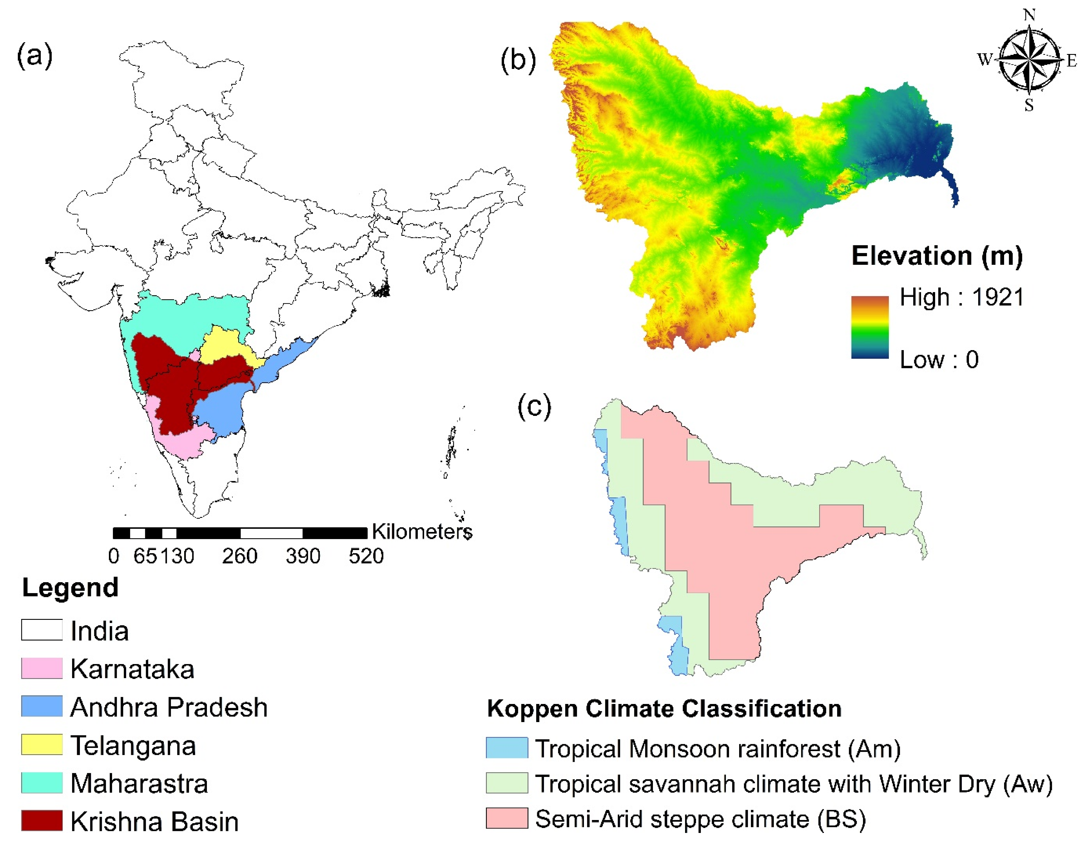
2.1. Study Area

KRB, the second largest in peninsular India, originates in the Western Ghats Region of Mahabaleshwar town at an elevation of about 1337 m above mean sea level [41]. The river is situated between 73°15′ to 81°20′E longitudes and 13°5′ to 19°20′N latitudes. KRB has a drainage area of ~258,998 km2 traversing with a length of 1400 km through the states of Andhra Pradesh, Telangana, Karnataka, and Maharashtra, as shown in Figure 1.
The major tributaries of KRB are Tungabhadra, Malaprabha, Koyna, and Bhima rivers [42]. Dominant soils found in this region are black soils, mixed soils, saline and alkaline soils, alluvium, and red soils. Much of the basin falls under a semi-arid climatic zone with massive occupancy of agricultural lands (76%). The majority of rainfall (90%) occurs during monsoon (June–October), with an average annual rainfall of 780 mm [43]. The maximum temperature varies between 20° and 42 °C, and the minimum temperature varies between 8° and 30 °C. The entire basin can be classified into three climatic zones as the Tropical Monsoon rainforest (Am), Tropical savannah climate with Winter Dry (Aw), and Semi-Arid steppe climate (BS) classification as per Koppen climate classification system. More details on the classification criteria implemented to segregate into different climatic zones in the Koppen system can be found in Chen and Chen (2013) and Kottek et al. (2006) [44,45].

2.2. Datasets Used

Four gridded precipitation products having 0.25° × 0.25° spatial resolution with a temporal resolution spanning from 1985 to 2018 were implemented in the current study. The four gridded SPPs employed in the present study are described below. The main reason for selecting these datasets is due to their long term and real-time availability, finer spatial resolution and their consistent performance that was reported in various studies [46,47,48,49,50].

2.2.1. ERA-5

The recently released ERA-5 dataset was developed from the ECMWF atmospheric reanalysis product. The dataset is available at a daily time step for a global scale with a resolution of 0.25° × 0.25°. The dataset was developed employing reanalysis procedures by implementing data from various model simulations across the world using different laws of physics. More details regarding the dataset development can be found in Copernicus Climate Change Service, 2017 [51]. The data was downloaded from https://cds.climate.copernicus.eu/.

2.2.2. Indian Meteorological Department (IMD)

IMD has developed a high-resolution daily rainfall gridded dataset of 0.25° × 0.25° for the entire Indian subcontinent. The Shepard Interpolation technique was implemented for interpolating all the precipitation values obtained from individual gauge stations. IMD used ~1803 gauge rainfall stations data for estimating 24-h accumulated rainfall. More details regarding IMD gridded data can be found in Pai et al. (2014) [52], and the data can be accessed from http://www.imdpune.gov.in/.

2.2.3. CHIRPS

Satellite and gauge-based rainfall estimates are provided by Climate Hazards Group Infrared Precipitation (CHIRP) product that has finer spatial resolution and longer periods. The CHIRPS (CHIRP blended with station data) datasets are developed by the University of California and USGS Geologic Survey that has a finer spatial resolution of 0.05° covering 50°N–50°S spanning from 1981. Different products like Climate Hazards Group Precipitation Climatology (CHPClim) having 0.05° resolution at monthly time scale estimated from station data, thermal infrared-based satellite rainfall estimates, Tropical Rainfall Measuring Mission (TRMM 3B42 v7) rainfall data, National Oceanic and Atmospheric Administration (NOAA) climate forecast system atmospheric rainfall data, and station-based precipitation data are blended and processed to produce CHIRPS rainfall data with high spatial and temporal resolution. The product so formed is of the penta-daily time step, which is then aggregated to a monthly time step. The present study uses CHIRPS data with 0.25° spatial resolution spanning for the years 1985 to 2018. More details regarding IMD gridded data can be found in Funk et al. (2015) [53], and the data can be accessed from the CHG portal or the mentioned FTP site (ftp://ftp.chg.ucsb.edu/pub/org/chg/products/).

2.2.4. Precipitation Estimation from Remotely Sensed Information Using Artificial Neural Networks-Climate Data Record (PERSIANN-CDR)

The need for long-term rainfall records is addressed by the development of the PERSIANN-CDR product. PERSIANN-CDR has a spatial resolution of 0.25° covering 60°S to 60°N having a span from January 1983 to December 2018. Global precipitation estimates provided by the PERSIANN algorithm uses both Infrared satellite and passive microwave data from GEO and LEO satellites. The 3-h rainfall estimates are generated by applying the PERSIANN algorithm to GridSat B1 Infrared satellite observations. The PERSIANN algorithm finds out the relationship between microwave and infrared data based on a neural network approach, and this relation is applied to Infrared (IR) data to generate 3-h rainfall estimates. The 3-h precipitation estimates are then combined with the GPCP product to eradicate the biases in the product that produces an adjusted PERSIANN-B1 rainfall estimate. The so-formed 3-h precipitation estimates after bias correction are then accumulated to form daily PERSIANN CDR Product of spatial resolution 0.25°. More details regarding PERSIANN-CDR data can be found in Ashouri et al. (2015) [54], and the data can be accessed from http://chrsdata.eng.uci.edu/ portal.

3. Methodology

3.1. Implementation of Machine Learning Techniques

In the current study, Secondary Precipitation Estimate Merging using Machine Learning (SPEM2L) was carried out to find out the optimum MLA that can be employed for merging precipitation datasets to generate improved spatial precipitation values over a basin. Sixteen MLAs broadly classified under six MLMs represented in Figure 2 were implemented in the current study. All the MLMs were trained using MATLAB 2018a, on an Intel Core i7, 3.07GHz machine with 16 GB RAM. As this is a preliminary study to find the best MLA out of many existing algorithms to merge different precipitation datasets effectively, all the MLAs are trained with default hyperparameters. The hyperparameters are used to control the learning process of MLAs that are required to be specified before starting the learning process in a training phase. The hyperparameters are used to build relations or to fit an equation between input and output variables. For example, in the case of neural networks, the hyperparameters are the number of hidden units, activation function, number of neurons in each layer, etc. The hyperparameters employed in the current study are represented in Table 1. Various MLMs represented in Figure 2 were developed and evaluated in the selected study area.

3.1.1. Linear Regression based Models

Simplified Linear Regression (LR), Linear Regression algorithm with Interactions term (LR-I), Stepwise Linear Regression algorithm (LR-S), and Linear Regression algorithm with Robust fitting (LR-R) were categorized and used under LR based models. A “fitlm” function with different options in MATLAB was used for LR, LR-I, and LR-R algorithms. A simple linear regression algorithm with stepwise regression was implemented for the LR-S algorithm. The default ordinary least squares method was employed in the case of LR to fit the algorithm between secondary precipitation datasets (CHIRPS + ERA-5) and gauge-based gridded data (IMD). A “bisquare” robust fitting weighting function was implemented with default tuning constant for the LR-R algorithm to fit between satellite and gauge based gridded datasets. Along with intercept and linear terms, an interaction term is further added to fit the LR-I MLA.

3.1.2. Support Vector Machine Regression Models

SVMs are supervised learning techniques developed for classification problems; however, they can be implemented for regression as well. SVM has a significant advantage to avoid trapping in a local minimum and network overfitting. In SVM, a hyperplane is constructed in a higher-dimensional space to classify the data. A nonlinear function in SVM is implemented to map the input data to the higher dimensional space. Based on the classification technique of SVM, Support Vector Regression (SVR) is proposed. The error between the estimate and actual value is calculated using cost function in SVR, whereas a threshold value (є) is used to specify the distance between the boundary lines. Four SVR algorithms—SVR with linear kernel regression algorithm (SL), SVR with a Gaussian kernel regression function having a kernel scale of 0.61 for SVR with Fine Gaussian kernel (SF), 2.4 for SVR with medium Gaussian kernel (SM), and 9.8 for SVR with coarse Gaussian kernel (SC)—were implemented in the study. The function “fitrsvm” in MATLAB was used for SL, SF, SM, and SC algorithms [55].

3.1.3. Regression Tree Models

In the case of regression trees, each dataset has undergone recursive binary portioning at the nodes, and the relationship between the dependant response and predictor variables was explored. These regression tree-based algorithms, namely, Fine Tree (FT), Medium Tree (MT), and Coarse Tree (CT), were implemented using “fitrtree” function in MATLAB with minimum leaf sizes of 4, 12, and 36, respectively [56].

3.1.4. Ensemble Models

Regression Ensemble—Boosting (EBT) and bootstrap regression or Bagging (EBG) algorithms were employed in the current study. The “fitrensemble” function with “LSBoost” and “Bag” learner aggregation methods are implemented for EBT and EBG algorithms, respectively [56,57,58].

3.1.5. Neural Network Models

Neural Network-based Levenberg—Marquardt algorithm (NLM) and Bayesian Regularization algorithm (NBR) were constructed for minimizing the errors by employing the Multilayer Perceptron Neural network (MLPNN) architecture with Levenberg Marquardt [59,60] and Bayesian Regularization functions [61]. From the entire input data, 60% was used for training the networks, and the remaining 40% was used for testing and validation purposes. The MLPNN architecture consists of single input, hidden and output layers. The hidden layer consists of two/three neurons corresponding to two/three inputs of secondary precipitation datasets [62].

3.1.6. K-Nearest Neighbour Models

The “fitcknn” function in MATLAB with dependent options is used in the current study. The regression fit between SPPs and IMD gridded data was carried out by employing a single neighbor and Euclidean distance in the current study [63,64].

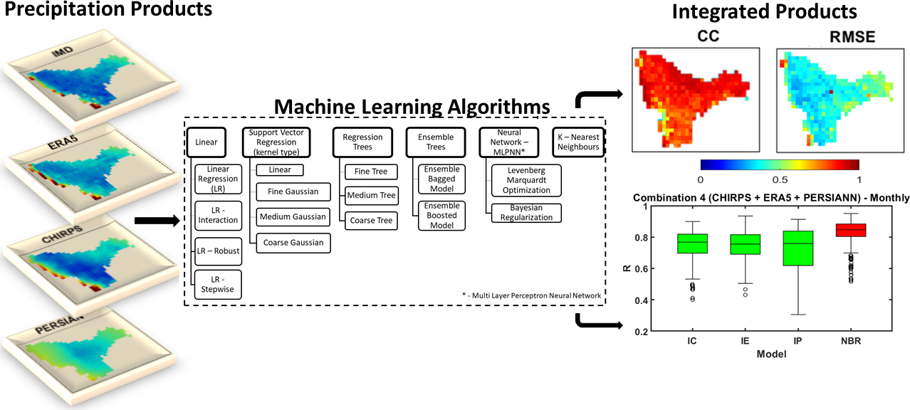
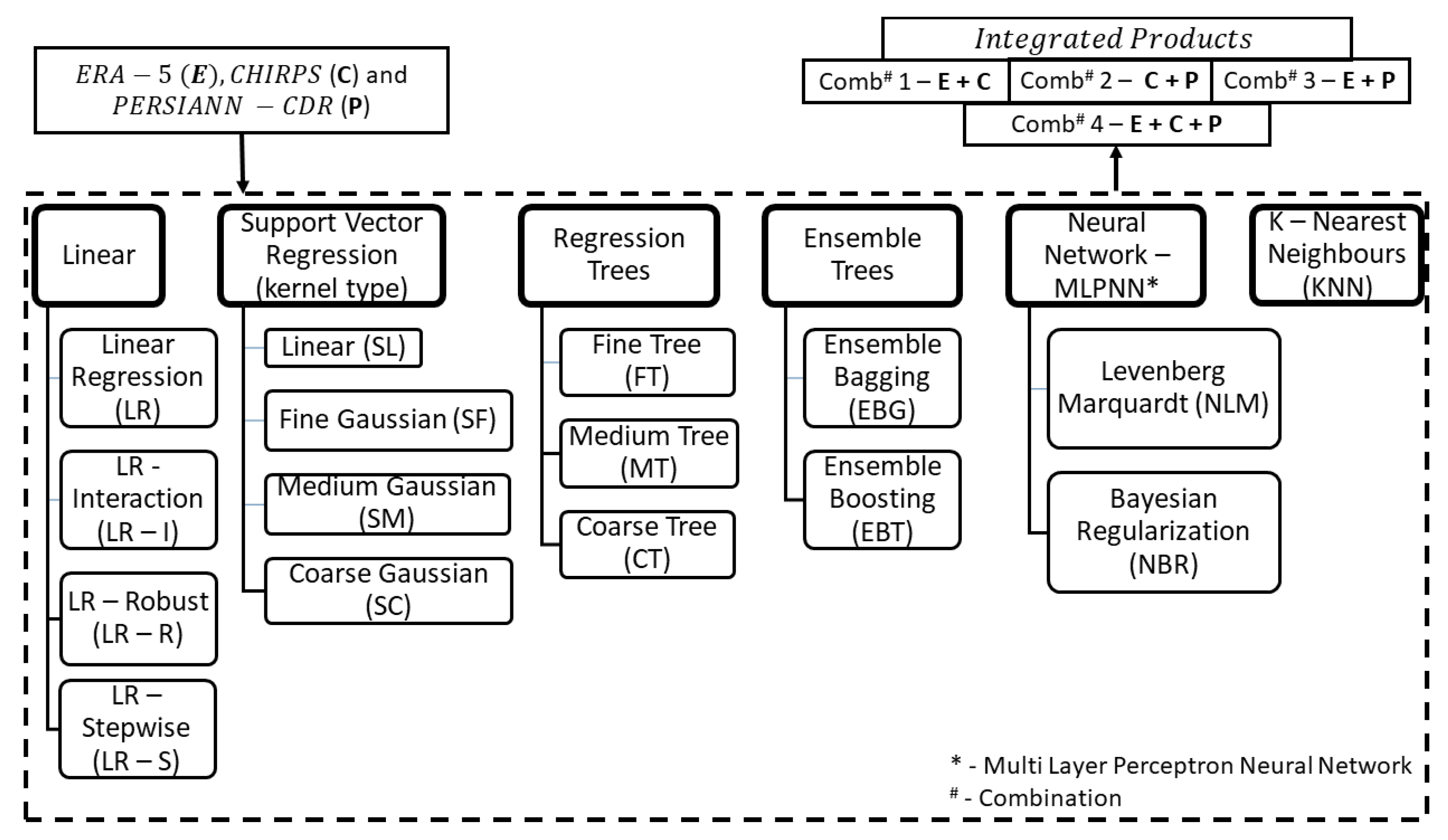
3.2. SPEM2L Procedure

The selected SPPs were divided into two groups: a training set (to train the MLMs) and a validation set (to evaluate the performance of the integrated product). In the current study, 34 years of precipitation data spanning from 1985 to 2018 was considered for merging precipitation datasets using MLAs. Out of these 34 years, 22 years (1985–2006) of data were considered for training the MLAs, whereas the other 12 years (2007–2018) of rainfall data were employed for testing and validation purposes. The continuous rainfall data was considered for training and testing to ensure that the minimum and maximum precipitation values that occur over summer and monsoon seasons are equally covered during training, testing, and validation phases. All the precipitation datasets are resampled to the same spatial (0.25°) and temporal resolution (daily) and to the same grid location as of IMD to ensure similar raster geometry. The SPPs were resampled by employing a cubic spline interpolation algorithm in MATLAB. During the training phase, all the MLMs were trained on the training subset implementing supervised regression between the SPPs and the IMD gridded data. As three SPPs are selected as an input, four combinations are developed to merge different SPPs and to evaluate against IMD gridded data:
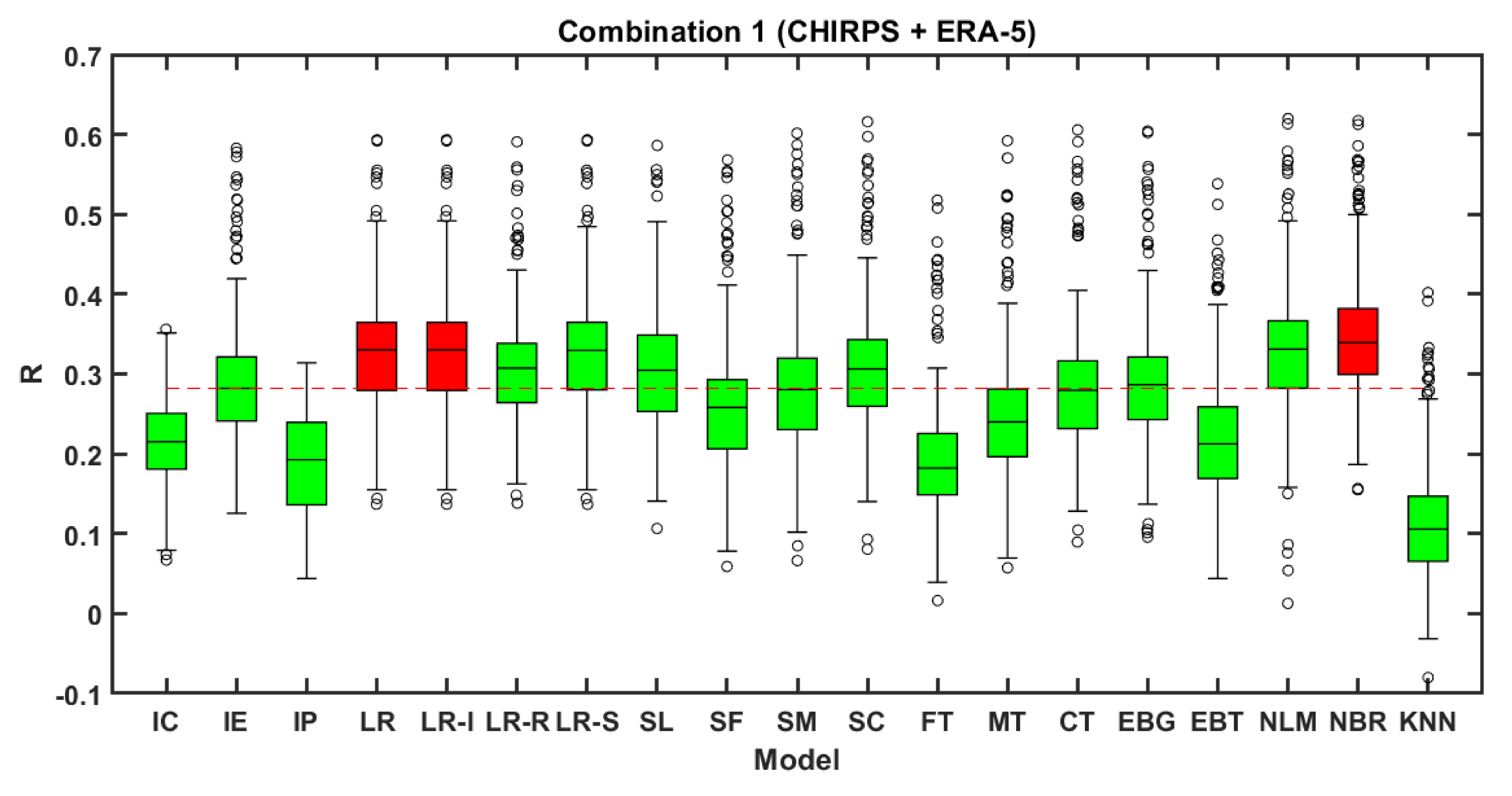
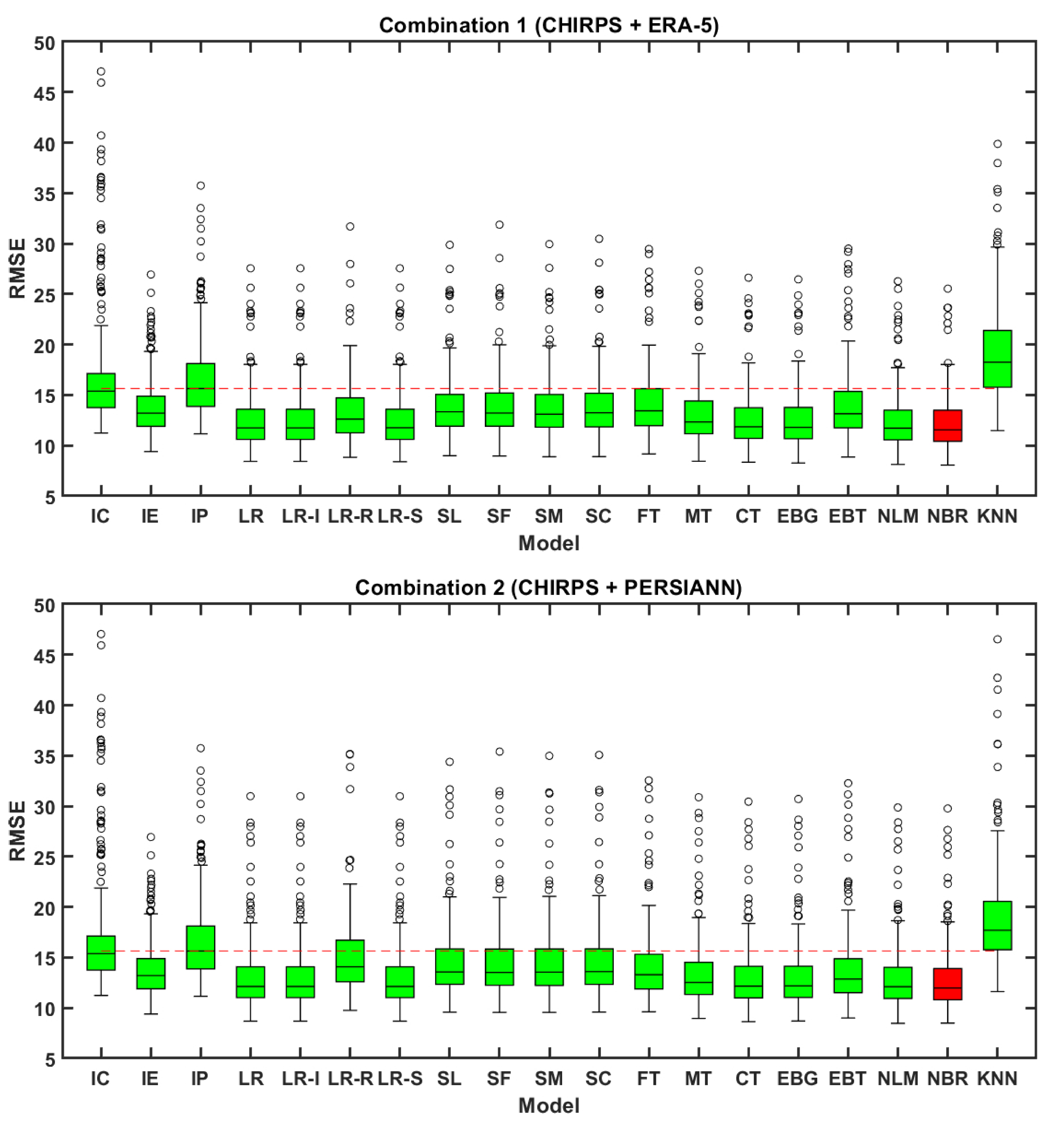
  • Combination 1: CHIRPS and ERA-5 precipitation datasets were merged employing sixteen MLAs and evaluated against IMD gridded data.
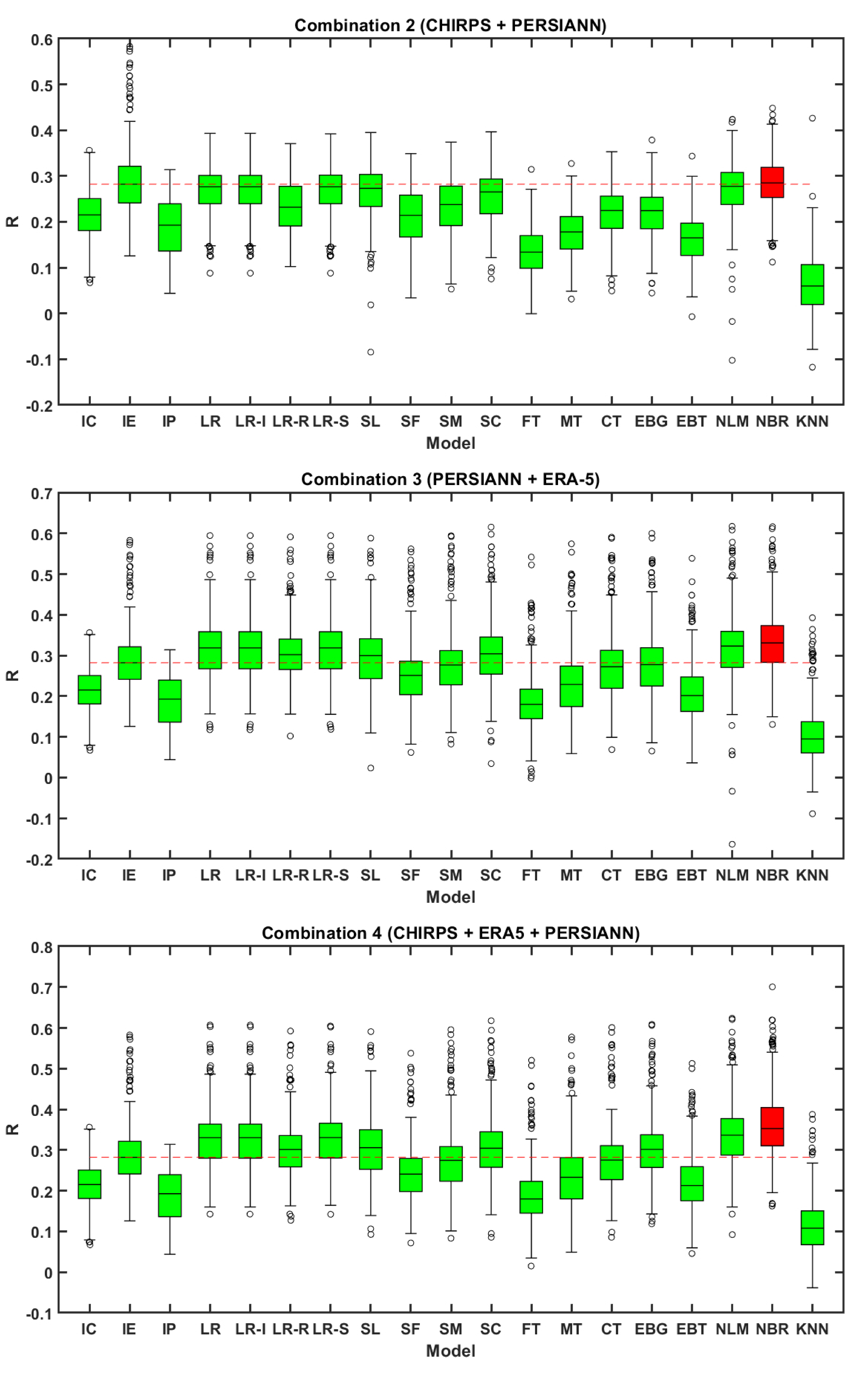
  • Combination 2: CHIRPS and PERSIANN-CDR SPPs were merged and evaluated against IMD.
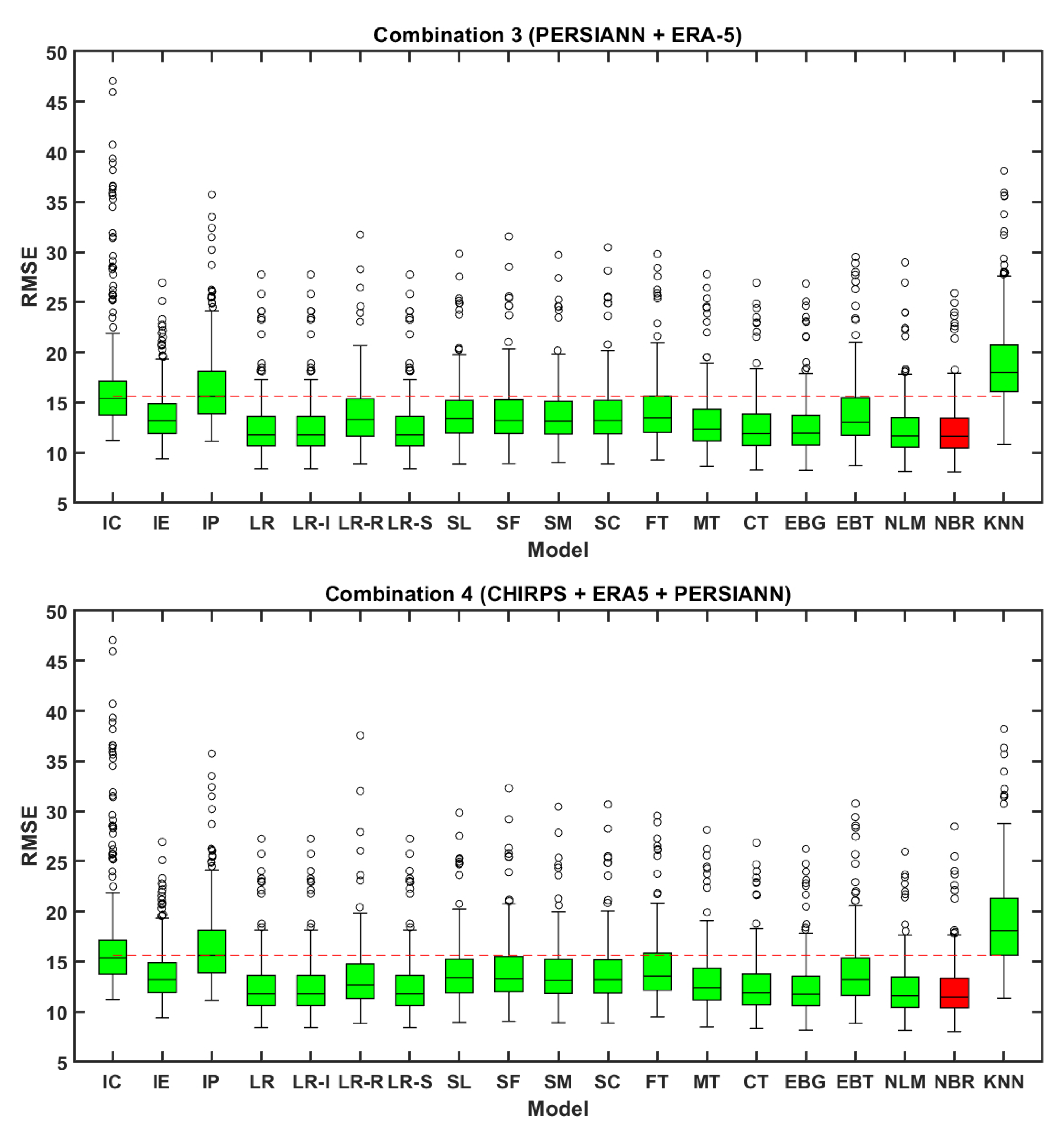
  • Combination 3: PERSIANN-CDR and ERA-5 SPPs were merged and evaluated against IMD.
  • Combination 4: All three SPPs were integrated (CHIRPS + ERA-5 + PERSIANN-CDR) and evaluated against IMD.
To carry out these combinations, first, the precipitation values at each grid cell are extracted for the entire period (1985–2018). Second, for each day, an MLA was trained for the years 1985–2006 using the selected SPPs in each combination as the dependent variable, and the precipitation values from IMD data as predictors. Third, the trained MLA was used to predict the daily precipitation values for each pixel of the study area for the remaining years (2007–2018). This process was repeated for each day for the years 1985–2018, employing all sixteen algorithms.

3.3. Performance Evaluation

Statistical analysis was performed to compare each SPP and the integrated products against IMD gridded data by employing categorical and continuous statistics that communicates the detection capabilities and error characteristics of SPPs. Probability of Detection (POD), False Alarm Ratio (FAR) categorized under categorical statistics, Correlation Coefficient (R), and Root Mean Square Error (RMSE) grouped under continuous statistics were employed in the current study for comparison. The categorical metrics convey the precipitation detection potentiality of SPPs. In contrast, the continuous metrics disclose the performance of SPP in estimating the amount of precipitation accurately when compared with the standard dataset (IMD). The ratio of hits (when SPP accurately detected the rainfall event concerning standard dataset) to the actual number of precipitation events occurred according to the base dataset is represented by POD. The ratio of misses (when SPP detects the rainfall event during the absence of rainfall in the standard dataset) to the actual number of rainfall events that are not diagnosed by the reference dataset is represented by FAR. A threshold of 1 mm/day was implemented for computing POD and FAR in the study. The categorical metrics were computed for the entire time series and it was segregated for different rainfall regimes. The precipitation intensities were partitioned into multiple rainfall regimes as low, medium, and high based on the criteria mentioned in Table 2.
The degree of relevance in precipitation between SPP and the gauge-based dataset is represented by R, RMSE indexes, or the averaged error magnitude between the SPP and the standard dataset. Higher R and lower RMSE represents greater accuracy of SPP in terms of detecting precipitation concerning base or standard datasets. More details regarding the metric and formulas can be found in Anjum et al. (2019), Wang et al. (2019), and Venkatesh et al. (2020) [65,66,67].

4. Results and Discussion

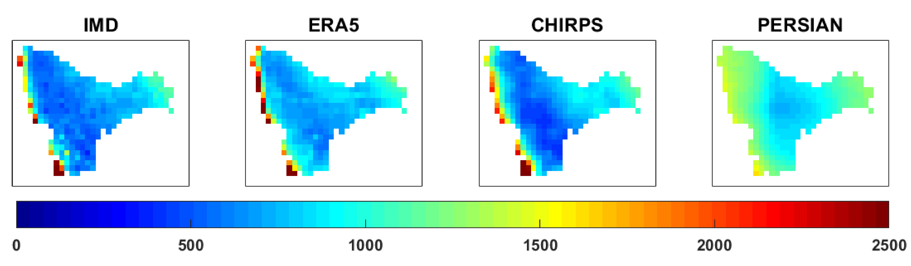
4.1. Spatial Pattern Assessment of the Rainfall Products

The spatial maps of average annual precipitation computed employing 34 years of precipitation data from IMD, CHIRPS, PERSIANN-CDR, and ERA-5 datasets for the Krishna River Basin in India are represented in Figure 3. From Figure 3, it can be observed that the average annual rainfall recorded by standard dataset (IMD) varies from 300 to 3000 mm throughout the basin. From Figure 1 and Figure 3, it can be noticed that high rainfall patterns were concentrated over the hilly regions of the basin that are having an elevation higher than 1000 m above mean sea level. Low rainfall pattern was recorded in the central part of the basin that falls under the semi-arid climatic zone (Figure 1 and Figure 3). A medium amount of rainfall ranging from 1000 to 1500 mm was concentrated at the mouth portion of the basin. Figure 3 illustrates that the western part of the basin classified under the tropical climatic zone recorded the highest amount of rainfall in all datasets due to the orographic effect of precipitation that occurs due to the occupancy of the Western Ghats mountains in the upper part of the basin. PERSIANN-CDR underestimated the amount of rainfall throughout the basin when compared to IMD with the average annual rainfall ranging from 800 to 1400 mm. The ERA-5 dataset contributed to an equal amount of precipitation (approximately 30–3000 mm) concerning IMD over the entire watershed. The CHIRPS dataset reported an underestimation with lower precipitation amounts in the central portion of the basin compared to the IMD dataset (Figure 3).

4.2. Evaluation of Machine Learning Models Performance at Daily Time Step

4.2.1. Combination 1

Combination 1 deals with the integration of CHIRPS and ERA-5 SPPs. The individual dataset comparison of CHIRPS and ERA-5 SPP with IMD resulted in a median R of 0.21 and 0.28 and a median RMSE of 15.38 and 13.2 mm/day, respectively (Figure 4 and Figure 5). After integration, eight algorithms (NBR, LR, LR-I, LR-R, LR-S, SL, SC, and NLM) resulted in increased median R-values and decreased RMSE values concerning base median values of CHIRPS and ERA-5 datasets. NLM, NBR, LR, and LR-I exhibited the best performance with a median R-value of 0.33 and RMSE of 11.71 mm/day for NLM, 11.74 mm/day for LR and LR-I, and 11.54 mm/day for NBR. The KNN algorithm exhibited poor performance with a median R-value of 0.1 and RMSE of 18.25 mm/day (Figure 4 and Figure 5). The boxplot (Figure 4 and Figure 5) with red color indicates the best-performed model and the red dotted line indicates the highest median (R/RMSE) obtained from the three individual precipitation datasets (ERA-5, PERSIANN-CDR, and CHIRPS). Combination 1 (Figure 4) resulted in a same R-value for three algorithms (LR, LR-I, and NBR) and thus the three boxplots were marked in red color.

4.2.2. Combination 2

Combination 2 deals with the integration of CHIRPS and PERSIANN-CDR SPPs. The individual dataset comparison of CHIRPS and PERSIANN-CDR with IMD resulted in a median R-value of 0.21 and 0.19 and a median RMSE of 15.38 and 15.64 mm/day, respectively, as shown in Figure 4 and Figure 5. After integration, 11 algorithms (LR, LR-I, LR-R, LR-S, SL, SM, SC, CT, EBG, NLM, and NBR) resulted in increased median R-values and decreased RMSE values concerning base median values of CHIRPS and PERSIANN-CDR. NBR exhibited the best performance with a median R-value of 0.28 and an RMSE of 11.97 mm/day. The KNN algorithm exhibited poor performance with a median R-value of 0.07 and RMSE of 17.69 mm/day (Figure 4 and Figure 5). Comparable performance was achieved by LR, LR-I, LR-S, SL, and NLM with median R-values of 0.27 and median RMSEs of ~12 mm/day. It can also be observed that the integrated algorithms and individual ERA-5 dataset resulted in a similar median of R and RMSE values. These results suggest that ERA-5 can be employed in a basin instead of integrating CHIRPS and PERSIANN-CDR datasets. This conclusion should further be validated in other basins/regions having different climatic and topographic patterns to frame as a standard conclusion.

4.2.3. Combination 3

Combination 3 deals with the merging of PERSIANN-CDR and ERA-5 precipitation datasets. The individual dataset comparison of PERSIANN-CDR and ERA-5 with IMD resulted in a median R of 0.19 and 0.28 and a median RMSE value of 15.64 and 13.24 mm/day, respectively, as shown in Figure 4 and Figure 5. After integrating implementing MLAs, eight algorithms (LR, LR-I, LR-R, LR-S, SL, SC, NLM, and NBR) resulted in increased median R-values and decreased RMSE values concerning base median values of PERSIANN-CDR and ERA-5. NBR exhibited the best performance with median R and RMSE values of 0.33 and 11.63 mm/day, respectively. KNN exhibited poor performance with lower R (0.09) and higher RMSE (18 mm/day) values (Figure 4 and Figure 5). The comparable performance was achieved by NLM next to NBR with a median R and RMSE values of 0.32 and 11.66 mm/day, respectively.

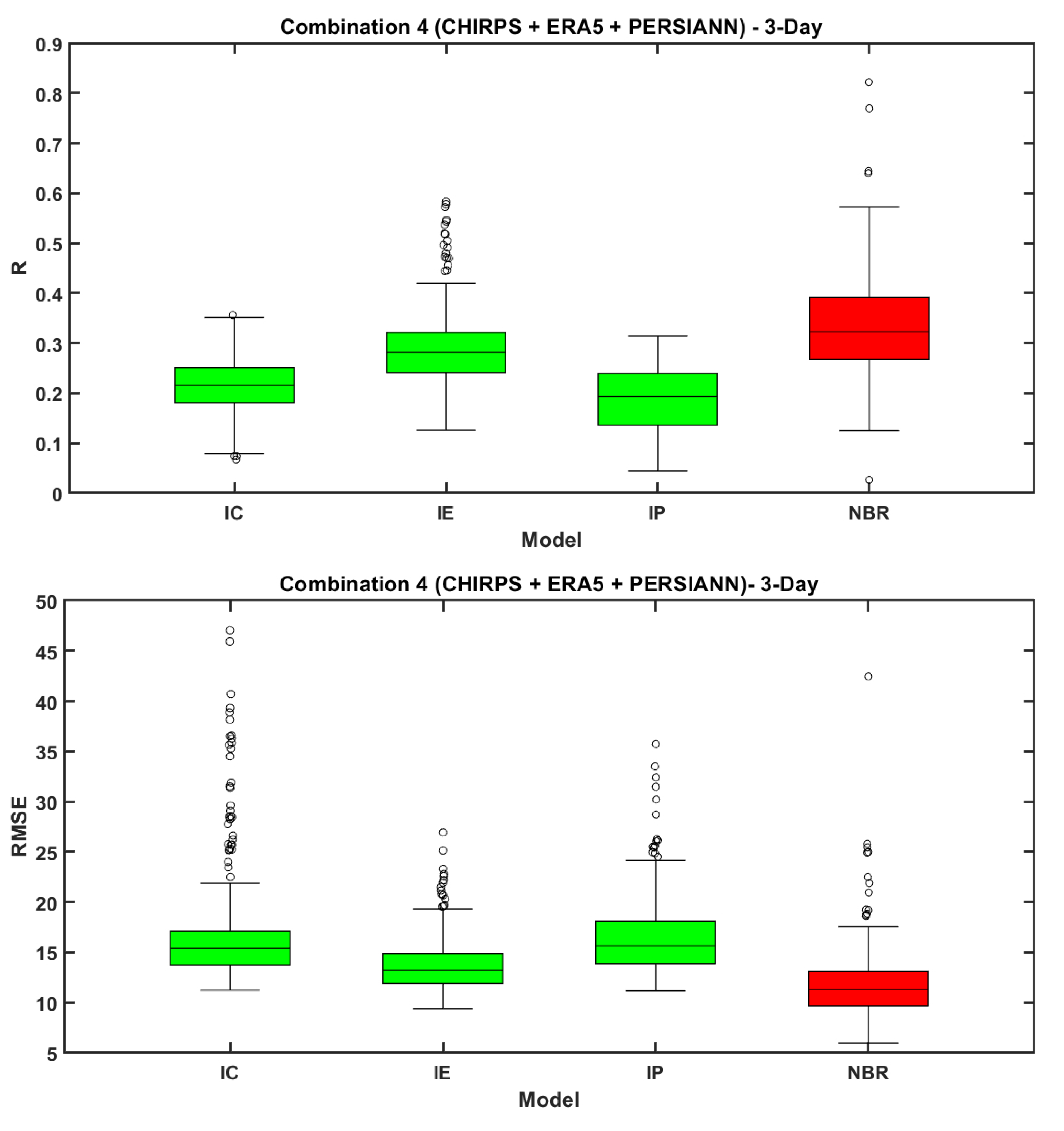
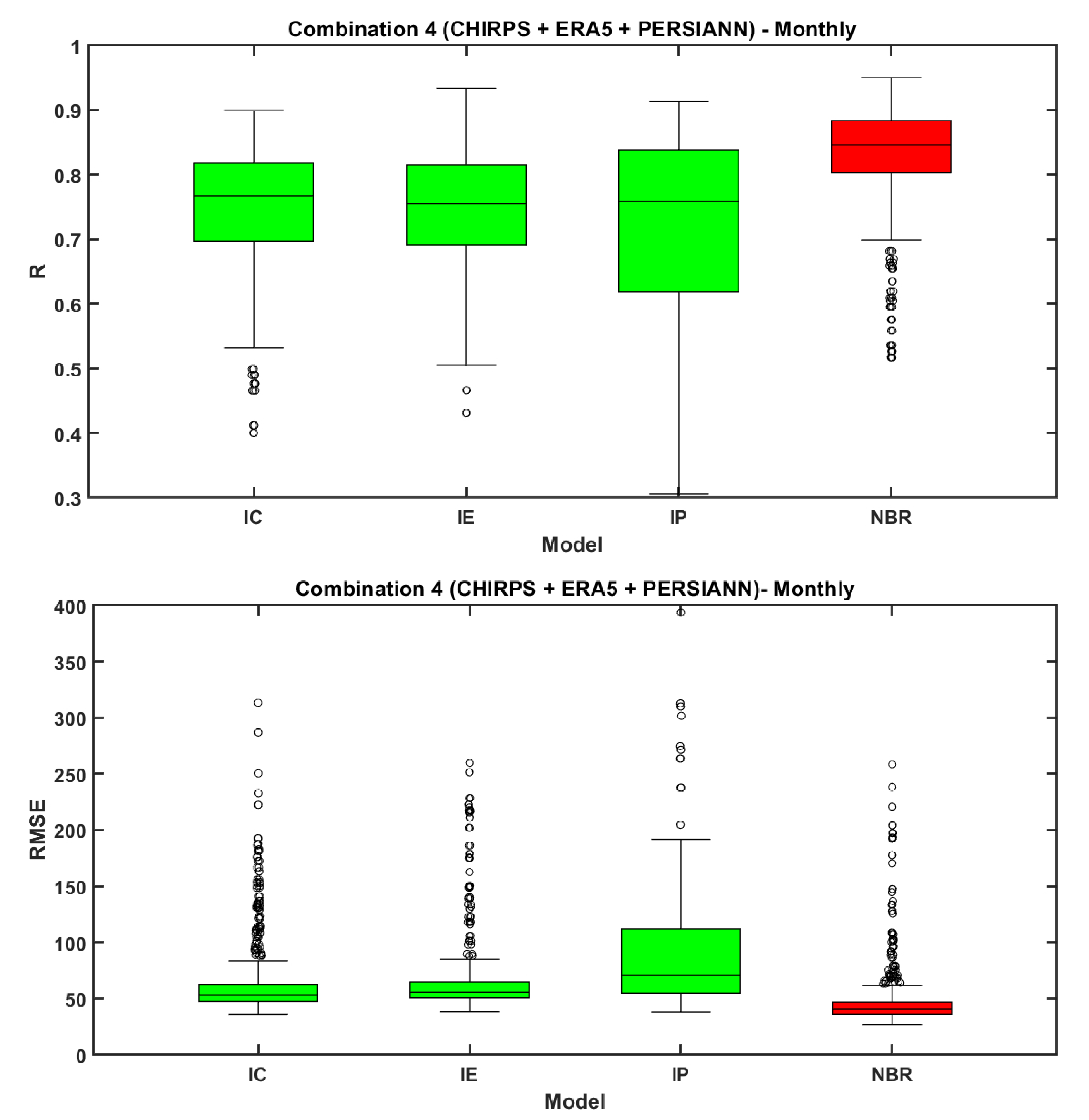
4.2.4. Combination 4

Combination 4 deals with the merging of all the three datasets employing MLAs. CHIRPS, ERA-5 and PERSIANN-CDR individual datasets when compared with IMD, a median correlation of 0.21, 0.28, and 0.19 and median RMSE of 15.38, 13.2, and 15.64 mm/day were observed. After merging employing MLAs, nine algorithms (LR, LR-I, LR-R, LR-S, SL, SC, EBG, NLM, and NBR) resulted in improved median R-values and decreased RMSE values concerning base median values of ERA-5, CHIRPS and PERSIANN-CDR datasets. The best performance in combination 4 was exhibited by NBR with a median R-value of 0.35 and RMSE of 11.46 mm/day, as shown in Figure 4 and Figure 5. KNN, as usual, resulted in poor performance with a median R-value of 0.1 and a median RMSE of 18.07 mm/day (Figure 4 and Figure 5). The comparable performance was achieved by LR, LR-I, LR-S, and NLM next to NBR with a median R-value of 0.33 and RMSE of 11.77 mm/day. From the individual comparison results of three SPPs with IMD, ERA-5 proved better when compared to CHIRPS and PERSIANN-CDR with lower error (RMSE) and higher correlation (R). The combinations that involved ERA-5 (CHIRPS + ERA-5 or PERSIANN + ERA-5) exhibited better performance than the combination that is having the other two datasets (CHIRPS + PERSIANN-CDR).
From the results of four combinations, it can be clearly stated that NBR outperformed from all MLMs in all combinations when either two or three datasets are merged. NLM and LR resulted in a comparable performance next to NBR in all combinations (Figure 4 and Figure 5). The KNN algorithm proved ineffective for combining different rainfall datasets in all sets of combinations. These results suggest that neural networks have high capability in merging different rainfall datasets. The simplest LR even exhibited comparable performance with NBR, suggesting that LR can be applied if complex trees or neural networks cannot be modelled and applied. From these results, it can be concluded that the SPEM2L procedure was able to improve the spatiotemporal representation of precipitation by integrating multiple rainfall datasets. Our results exhibited that the blending of multiple precipitation estimates can improve the spatiotemporal characterization of rainfall, which is consistent with the results obtained by Manz et al. (2016) and Verdin et al. (2016) [68,69]. From the overall results, the NBR algorithm from combination 4 exhibited better performance when compared to the other 15 MLAs and three combinations. As NBR from combination 4 (hereafter called as NBRC-4) proved effective, further analysis in the manuscript was performed and discussed with NBRC-4 results.

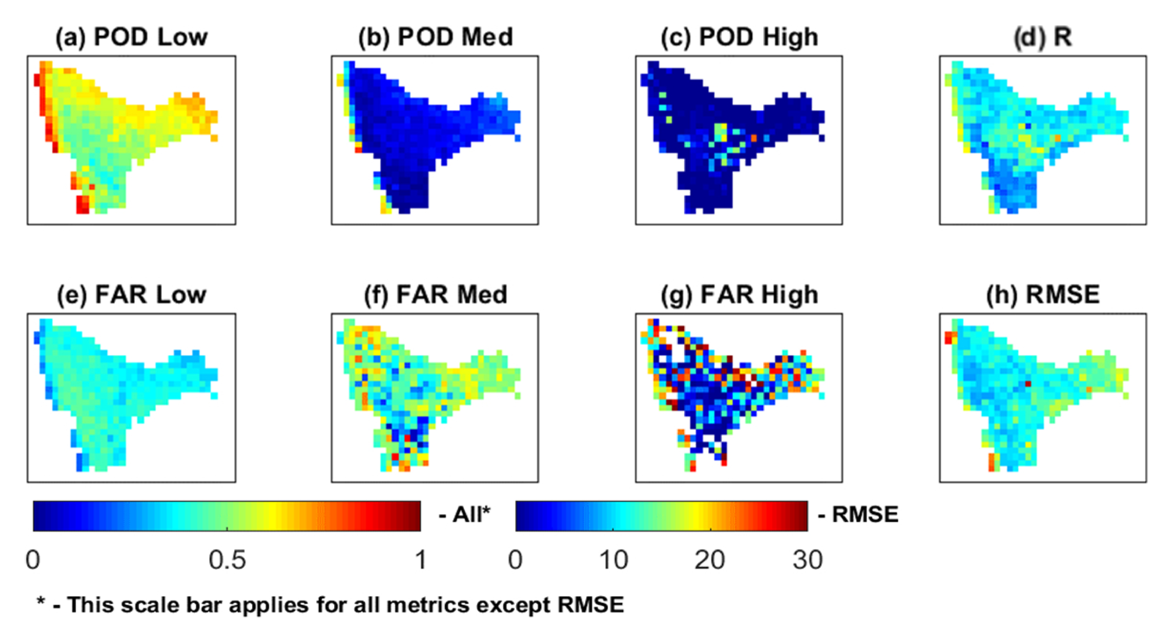
4.3. Categorical Metric Assessment

As the NBRC-4 algorithm performed better compared to individual datasets (ERA-5, PERSIANN-CDR, and CHIRPS) and other model combinations in continuous statistic assessment, the categorical statistical metric evaluation is discussed with the results obtained from NBRC-4 algorithm. Categorical statistics, i.e., POD and FAR, are computed based on the formulas mentioned in Table 2 and are segregated into low (0–5 mm), medium (5–25 mm), and high (>25 mm) rainfall classes. The pattern of POD and FAR for the NBRC-4 algorithm dataset computed against IMD is shown in Figure 6. The NBRC-4 algorithm has a high POD value (median of 0.572) in low rainfall criteria indicating better rainfall event detection at a daily time step. For medium and high rainfall intensities, the value of POD followed a declining trend (median of 0.09 and 0.009), indicating that the rainfall event detection capability decreases with the increase of rainfall intensity, as shown in Figure 6.
FAR, which should have a value closer to 0, indicated moderate rainfall detection capability at low rainfall events with a median value of 0.38. The NBRC-4 algorithm detected more false rainfall events in case of medium rainfall resulting in a median FAR value of 0.48. In the high rainfall intensity category, NBRC-4 performed better, detecting fewer false rainfall events (median value of 0.29) when compared with the IMD dataset (Figure 6). The POD values with 1 mm/day rainfall threshold exhibited that the overall rainfall detection skill of all datasets decreases as precipitation intensity increases, and vice versa for FAR metrics. These categorical assessment results reveal that all the implemented datasets cannot detect the magnitude of extreme precipitation events accurately. Similar results were reported by Ahmed et al. (2019) and Pour et al. (2014) [70,71], where they concluded that high magnitude or extreme rainfall occurs at a micro-level and therefore, the SPPs may not have the potentiality to detect those rainfall events accurately at the point level. In supporting this statement, Schneider et al. (2017) [72] commented that the SPPs could detect these extreme rainfall events when the gridded dataset is developed with forcing a more significant or dense number of observed station data over an area which we currently lack all around the world. From the overall categorical skill score test results, it can be observed that the NBRC-4 algorithm performed better in detecting low rainfall events compared to medium and high-intensity precipitation events.

4.4. Temporal Assessment of NBRC-4 Algorithm Performance

The performance of the NBRC-4 algorithm is assessed at a 3-day and monthly time step by applying continuous statistic metrics (R and RMSE). The performance of individual datasets (ERA-5, PERSIANN-CDR, and CHIRPS) at a 3-day time step is similar to that of a daily time step that has a median R-value of 0.21, 0.28, and 0.19 and median RMSE value of 15.38, 13.2, and 15.64 mm/3-day respectively (Figure 7). The NBRC-4 algorithm proved best even at a 3-day time step with a median R of 0.32 and RMSE of 11.28 mm. At a monthly time frame, individual datasets (ERA-5, PERSIANN-CDR, and CHIRPS) exhibited a high correlation with a median R-value of 0.76, 0.75, and 0.75 and higher RMSE values of 53.36, 55.76, and 70.7 mm/month, respectively. However, the NBRC-4 algorithm outperformed even at a monthly time step with a median R and RMSE values of 0.84 and 40.5 mm/month, respectively, as shown in Figure 7. The evaluated merged precipitation products exhibited higher performances at the monthly time scales in comparison to shorter temporal scales (daily), similar to the results reported by Jiang et al. (2012) and Zambrano-Bigiarini et al. (2017) [73,74]. This represents that despite systematic, random, and detection errors present in precipitation datasets at the daily time step, they are still able to describe precipitation patterns when aggregated at longer temporal scales (monthly).

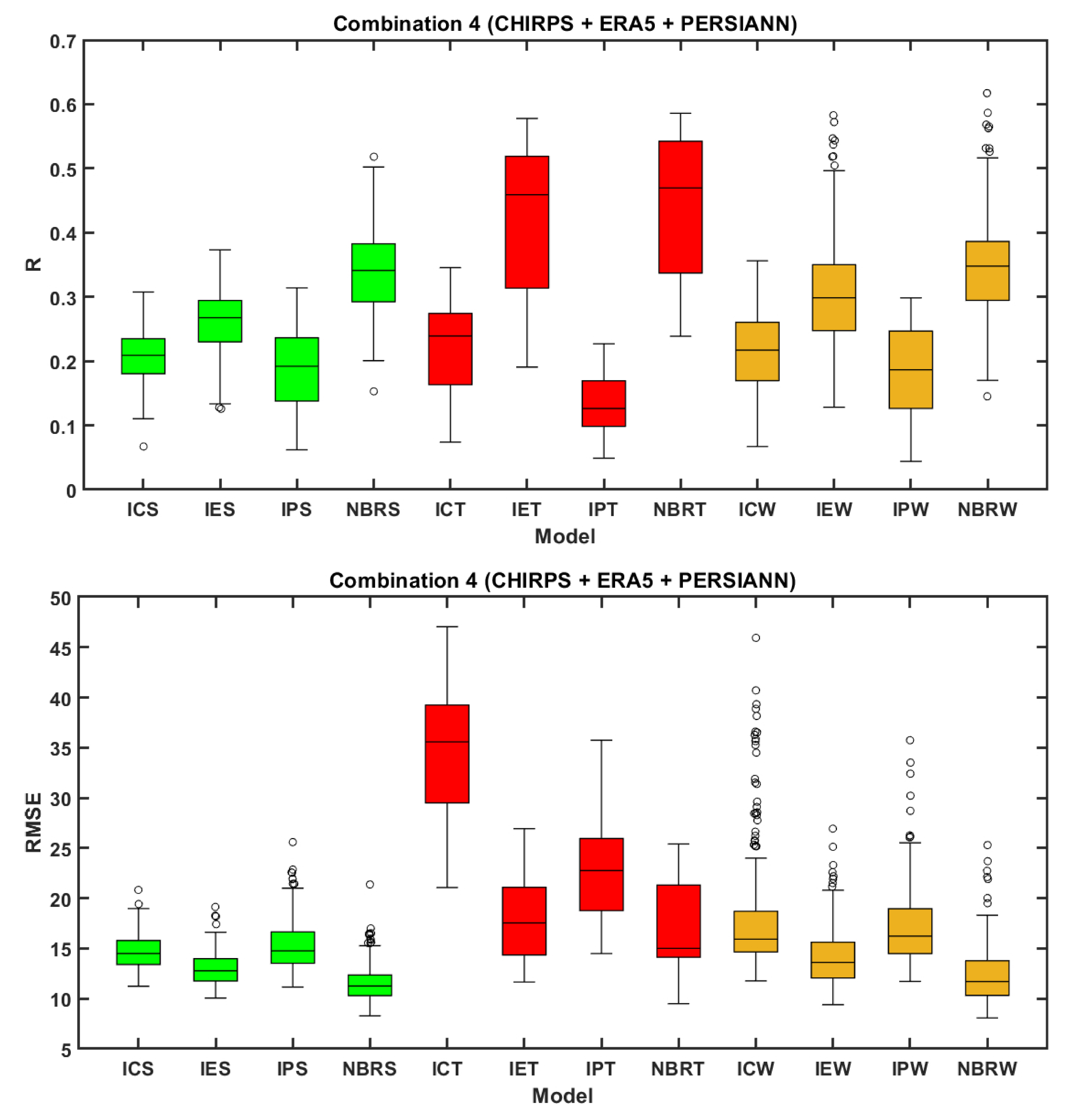
4.5. Performance Assessment of NBRC-4 Algorithm in Various Climatic Zones

The Krishna River Basin (KRB) employed in the current study comprises three climatic zones, i.e., Tropical Monsoon rainforest (Am), Tropical savannah climate with Winter Dry (Aw), and Semi-Arid Steppe climate (BS), as shown in Figure 1.
The performance of the NBRC-4 algorithm was assessed in the three climatic zones using continuous statistics. From Figure 8, it can be observed that NBRC-4 outperformed when compared to individual SPPs comparisons with IMD in TM climatic zone, projecting a median R-value of 0.49 and RMSE of 15.04 mm/day. In the case of BS climatic zone, NBRC-4 provided better results (median R of 0.34 and median RMSE of 11.26 mm/day) compared to other SPPs with median R values of 0.2, 0.26, and 0.19 and median RMSE values of 14.51, 12.78, and 14.76 mm/day for CHIRPS, ERA-5 and PERSIANN-CDR, respectively. A similar pattern of results was observed in the Aw climatic zone, where NBRC-4 proved effective with a median R of 0.34 and RMSE of 11.74 mm compared to other individual SPPs. Poor performance was observed from the statistical values of PERSIANN CDR with high error magnitudes (RMSE) when assessed at different temporal scales and climatic zones (Figure 8).
The poor performance of PERSIANN CDR may be attributed to the competent training of ANN over the United States and inadequate training of ANN over other parts of the world [75,76]. High error magnitudes (RMSE of 35.8 mm/day) were exhibited by the CHIRPS dataset in the Tropical Monsoon climatic region. Similar results have been reported earlier by Musie et al. (2019), Shrestha et al. (2017), and Tang et al. (2019) [77,78,79] while using CHIRPS dataset and the reason for the weaker performance may be attributed to the Infrared algorithm (which computes data from Infrared region retrieved signals) that was used for CHPClim dataset developments which implement fixed brightness temperature thresholds to differentiate raining and non-raining clouds. The defined thresholds are usually too cold and the orographic precipitation occurring over the Western Ghats was warm which may not produce much ice aloft resulting in an underestimation of rainfall [77,80,81,82,83,84]. The pattern of the RMSE statistical metric is like that of R, where ERA-5 revealed better results than CHIRPS and PERSIANN-CDR. From the overall results of continuous statistics at a daily time step, ERA-5 yielded better results than CHIRPS and PERSIANN-CDR in all climatic regions with high R and low RMSE values. From the overall results related to the assessment of the NBRC-4 algorithm in contrasting climatic zones, it is observed that the NBRC-4 algorithm outperformed when compared to individual dataset statistical performance.
Although the SPEM2L procedure was only applied over the KRB, we are confident that this method could be successfully applied over other basins or regions that are ungauged or have a poor gauging network, due to its effective performance in a region with notable heterogeneity in topography and climate; and because it was able to improve the spatiotemporal characterization of precipitation. Future studies can implement hyperparameter tuning and optimization for obtaining more effective results when implementing the NBR algorithm for merging different datasets. Researchers can further implement and test this NBR algorithm in different climatic and topographic regions for merging different SPPs to frame a standard framework for generating accurate precipitation products that can be used for monitoring and predicting natural hazards. Apart from the employed SPPs in the current study, different precipitation products should be implemented and merged based on their availability to test the efficiency of NBR algorithm for merging different SPPs. The merged precipitation product can further be implemented in a hydrological model to test its efficiency in simulating water balance components accurately compared to individual precipitation dataset simulations.

5. Conclusions

Secondary precipitation products furnish an exceptional anomalous opportunity for various hydro-meteorological and environmental applications. Despite the continuous improvements of rainfall datasets, still, the datasets are prone to biases and mismatches. To overcome some of those biases, here we presented a novel SPEM2L framework that is capable of deriving improved precipitation estimates by merging secondary rainfall datasets alone that are publicly available for the entire globe with near-real-time precipitation estimates. Neural network-based algorithms (NLM and NBR) and linear regression-based algorithms (LR, LR-I, and LR-S) developed with the proposed method exhibited improved rainfall characterization at all temporal scales and contrasting climatic zones compared to the individual precipitation datasets. Finally, the NBR algorithm with three dataset integration performed better than other combinations and other 15 MLA’s. Some of the key findings from this applied methodology are mentioned below.
  • ERA-5 yielded better statistical results than CHIRPS and PERSIANN-CDR in all climatic zones with high correlation and low magnitude of errors (RMSE).
  • The POD and FAR statistics exhibited that the overall rainfall detection skill of all datasets decreases as precipitation intensity increases.
  • The individual precipitation products and the MLA’s exhibited superior performance at longer timescales (monthly) than at shorter spans (daily).
  • NBRC-4, which employs three-dataset merging, performed better than all other combinations that involve two rainfall dataset integration.
  • NBRC-4 algorithm outperformed than all the evaluated rainfall products at different temporal resolutions (daily, 3-day, and monthly) and climatic zones (Am, Aw, and BS).
  • The amplification of RMSE can be observed from arid to tropical climatic zones in all the tested precipitation datasets.
  • SPEM2L procedure can be applied at different temporal scales (i.e., daily, 3-day, and monthly) to acquire an improved spatiotemporal rainfall characterization.
SPEM2L was proposed and tested in a heterogeneous catchment (KRB) that has varying climate and topography with publicly available global datasets. The proposed methodology improved the spatiotemporal characterization of rainfall, and hence the authors are confident that this framework can be applied for any region or basin that has a poor gauging network or where a single precipitation product is testing ineffective. The current research gives an insight to the researchers to select suitable MLAs for integrating multiple precipitation datasets along with the best dataset that can be employed in any region for hydrological and climatological applications.

Author Contributions

Conceptualization, V.K.; Data curation, V.K. and S.K.; Formal analysis, V.K., S.K., and T.D.A.; Investigation, V.K. and N.W.; Methodology, V.K.; Resources, S.K.; Software, S.K.; Supervision, T.D.A.; Validation, V.K.; Visualization, V.K.; Writing—original draft, V.K.; Writing—review and editing, N.W. and T.D.A. All authors have read and agreed to the published version of the manuscript.

Funding

This research received no external funding and the APC was funded by MDPI.

Acknowledgments

The authors are very thankful to all the organizations and institutes that developed precipitation datasets and made them available for free.

Conflicts of Interest

The authors declare no conflict of interest.

Data and Code Availability

Datasets used in the study are freely available and can be accessed from the literature in [51,53,54] for PERSIANN-CDR, ERA-5, and CHIRPS datasets, respectively. They can be downloaded from https://cds.climate.copernicus.eu/, ftp://ftp.chg.ucsb.edu/pub/org/chg/products/, and http://chrsdata.eng.uci.edu/ portals for ERA-5, CHIRPS, and PERSIANN-CDR datasets, respectively. The code can be obtained by contacting the first author directly at [email protected].

Abbreviations

ANNArtificial Neural Network
CHIRPSClimate Hazards Group InfraRed Precipitation with Station
ERA-5ECMWF (European Centre for Medium-Range Weather Forecasts) ReAnalysis
FARFalse Alarm Ratio
IMDIndian Meteorological Department
KRBKrishna River Basin
MLAMachine Learning Algorithm
MLMMachine Learning Model
NBRC-4Neural Network-based Bayesian Regularization algorithm results from Combination 4
PODProbability of Detection
PERSIANN-CDRPrecipitation Estimation from Remotely Sensed Information using Artificial Neural Networks-Climate Data Record
SM2RAIN-CCISoilMoisture2RAIN-Climate Change Initiative
SPEM2LSecondary Precipitation Estimate Merging using Machine Learning
SPPSecondary Precipitation Product
SVMSupport Vector Machine
TRMMTropical Rainfall Measuring Mission

References

  1. Woldemeskel, F.M.; Sivakumar, B.; Sharma, A. Merging gauge and satellite rainfall with specification of associated uncertainty across Australia. J. Hydrol. 2013, 499, 167–176. [Google Scholar] [CrossRef]
  2. Beusch, L.; Foresti, L.; Gabella, M.; Hamann, U. Satellite-based rainfall retrieval: From generalized linear models to artificial neural networks. Remote Sens. 2018, 10, 939. [Google Scholar] [CrossRef] [Green Version]
  3. Mazzetti, C.; Todini, E. Combining Raingages and Radar Precipitation Measurements Using a Bayesian Approach. Geoenv IV Geostat. Environ. Appl. 2006, 10, 401–412. [Google Scholar] [CrossRef]
  4. Todini, E. A Bayesian technique for conditioning radar precipitation estimates to rain-gauge measurements. Hydrol. Earth Syst. Sci. 2001, 5, 187–199. [Google Scholar] [CrossRef] [Green Version]
  5. Bitew, M.M.; Gebremichael, M. Evaluation of satellite rainfall products through hydrologic simulation in a fully distributed hydrologic model. Water Resour. Res. 2011, 47, 1–11. [Google Scholar] [CrossRef]
  6. Thiemig, V.; Rojas, R.; Zambrano-Bigiarini, M.; de Roo, A. Hydrological evaluation of satellite-based rainfall estimates over the Volta and Baro-Akobo Basin. J. Hydrol. 2013, 499, 324–338. [Google Scholar] [CrossRef]
  7. Xue, X.; Hong, Y.; Limaye, A.S.; Gourley, J.J.; Huffman, G.J.; Khan, S.I.; Dorji, C.; Chen, S. Statistical and hydrological evaluation of TRMM-based Multi-satellite Precipitation Analysis over the Wangchu Basin of Bhutan: Are the latest satellite precipitation products 3B42V7 ready for use in ungauged basins? J. Hydrol. 2013, 499, 91–99. [Google Scholar] [CrossRef]
  8. Yuan, F.; Wang, B.; Shi, C.; Cui, W.; Zhao, C.; Liu, Y.; Ren, L.; Zhang, L.; Zhu, Y.; Chen, T.; et al. Evaluation of hydrological utility of IMERG Final run V05 and TMPA 3B42V7 satellite precipitation products in the Yellow River source region, China. J. Hydrol. 2018, 567, 696–711. [Google Scholar] [CrossRef]
  9. Zhang, D.; Liu, X.; Bai, P.; Li, X.H. Suitability of satellite-based precipitation products for water balance simulations using multiple observations in a humid catchment. Remote Sens. 2019, 11, 151. [Google Scholar] [CrossRef] [Green Version]
  10. Yin, S.; Xie, Y.; Liu, B.; Nearing, M.A. Rainfall erosivity estimation based on rainfall data collected over a range of temporal resolutions. Hydrol. Earth Syst. Sci. 2015, 19, 4113–4126. [Google Scholar] [CrossRef] [Green Version]
  11. Teng, H.; Ma, Z.; Chappell, A.; Shi, Z.; Liang, Z.; Yu, W. Improving rainfall erosivity estimates using merged TRMM and gauge data. Remote Sens. 2017, 9, 1134. [Google Scholar] [CrossRef] [Green Version]
  12. Panagos, P.; Borrelli, P.; Meusburger, K.; Yu, B.; Klik, A.; Lim, K.J.; Yang, J.E.; Ni, J.; Miao, C.; Chattopadhyay, N.; et al. Global rainfall erosivity assessment based on high-temporal resolution rainfall records. Sci. Rep. 2017, 7, 1–12. [Google Scholar] [CrossRef] [PubMed] [Green Version]
  13. Bhatt, B.C.; Nakamura, K. Characteristics of monsoon rainfall around the Himalayas revealed by TRMM precipitation radar. Mon. Weather Rev. 2005, 133, 149–165. [Google Scholar] [CrossRef]
  14. Munzimi, Y.A.; Hansen, M.C.; Adusei, B.; Senay, G.B. Characterizing Congo basin rainfall and climate using Tropical Rainfall Measuring Mission (TRMM) satellite data and limited rain gauge ground observations. J. Appl. Meteorol. Clim. 2015, 54, 541–555. [Google Scholar] [CrossRef]
  15. John, R.; Chen, J.; Ou-Yang, Z.T.; Xiao, J.; Becker, R.; Samanta, A.; Ganguly, S.; Yuan, W.; Batkhishig, O. Vegetation response to extreme climate events on the Mongolian Plateau from 2000 to 2010. Environ. Res. Lett. 2013, 8, 035033. [Google Scholar] [CrossRef]
  16. Hoscilo, A.; Balzter, H.; Bartholomé, E.; Boschetti, M.; Brivio, P.A.; Brink, A.; Clerici, M.; Pekel, J.F. A conceptual model for assessing rainfall and vegetation trends in sub-Saharan Africa from satellite data. Int. J. Clim. 2015, 35, 3582–3592. [Google Scholar] [CrossRef] [Green Version]
  17. Pasetto, D.; Arenas-Castro, S.; Bustamante, J.; Casagrandi, R.; Chrysoulakis, N.; Cord, A.F.; Dittrich, A.; Domingo-Marimon, C.; El Serafy, G.; Karnieli, A.; et al. Integration of satellite remote sensing data in ecosystem modelling at local scales: Practices and trends. Methods Ecol. Evol. 2018, 9, 1810–1821. [Google Scholar] [CrossRef] [Green Version]
  18. Giglio, L.; Kendall, J.D.; Tucker, C.J. Remote sensing of fires with the TRMM VIRS. Int. J. Remote Sens. 2000, 21, 203–207. [Google Scholar] [CrossRef]
  19. Venkatesh, K.; Preethi, K.; Ramesh, H. Evaluating the effects of forest fire on water balance using fire susceptibility maps. Ecol. Indic. 2020, 110, 105856. [Google Scholar] [CrossRef]
  20. Haile, A.T.; Tefera, F.T.; Rientjes, T. Flood forecasting in Niger-Benue basin using satellite and quantitative precipitation forecast data. Int. J. Appl. Earth Obs. Geoinf. 2016, 52, 475–484. [Google Scholar] [CrossRef]
  21. Sharma, V.K.; Mishra, N.; Shukla, A.K.; Yadav, A.; Rao, G.S.; Bhanumurthy, V. Satellite data planning for flood mapping activities based on high rainfall events generated using TRMM, GEFS and disaster news. Ann. Gis 2017, 23, 131–140. [Google Scholar] [CrossRef]
  22. Kirschbaum, D.; Stanley, T. Satellite-Based Assessment of Rainfall-Triggered Landslide Hazard for Situational Awareness. Earths Futur. 2018, 6, 505–523. [Google Scholar] [CrossRef]
  23. Massari, C.; Brocca, L.; Moramarco, T.; Tramblay, Y.; Didon Lescot, J.F. Potential of soil moisture observations in flood modelling: Estimating initial conditions and correcting rainfall. Adv. Water Resour. 2014, 74, 44–53. [Google Scholar] [CrossRef]
  24. Ciabatta, L.; Brocca, L.; Massari, C.; Moramarco, T.; Puca, S.; Rinollo, A.; Gabellani, S.; Wagner, W. Integration of satellite soil moisture and rainfall observations over the italian territory. J. Hydrometeorol. 2015, 16, 1341–1355. [Google Scholar] [CrossRef]
  25. Fereidoon, M.; Koch, M.; Brocca, L. Predicting rainfall and runoff through satellite soil moisture data and SWAT modelling for a poorly gauged basin in Iran. Water. 2019, 11, 594. [Google Scholar] [CrossRef] [Green Version]
  26. Sinclair, S.; Pegram, G. Combining radar and rain gauge rainfall estimates using conditional merging. Atmos. Sci. Lett. 2005, 6, 19–22. [Google Scholar] [CrossRef]
  27. Huffman, G.J.; Adler, R.F.; Morrissey, M.M.; Bolvin, D.T.; Curtis, S.; Joyce, R.; McGavock, B.; Susskind, J. Global Precipitation at One-Degree Daily Resolution from Multisatellite Observations. J. Hydrometeorol. 2001, 2, 36–50. [Google Scholar] [CrossRef] [Green Version]
  28. Beck, H.E. Global-scale evaluation of 22 precipitation datasets using gauge observations and hydrological modeling. Hydrol. Earth Syst. Sci. 2017, 21, 6201–6217. [Google Scholar] [CrossRef] [Green Version]
  29. Bhuiyan, M.A.E.; Nikolopoulos, E.I.; Anagnostou, E.N.; Quintana-Seguí, P.; Barella-Ortiz, A. A nonparametric statistical technique for combining global precipitation datasets: Development and hydrological evaluation over the Iberian Peninsula. Hydrol. Earth Syst. Sci. 2018, 22, 1371–1389. [Google Scholar] [CrossRef] [Green Version]
  30. Duque-Gardeazábal, N.; Zamora, D.; Rodríguez, E. Analysis of the Kernel Bandwidth Influence in the Double Smoothing Merging Algorithm to Improve Rainfall Fields in Poorly Gauged Basins. EPiC Ser. Eng. 2018, 3, 635–642. [Google Scholar] [CrossRef] [Green Version]
  31. Heidinger, H.; Yarlequé, C.; Posadas, A.; Quiroz, R. TRMM rainfall correction over the Andean Plateau using wavelet multi-resolution analysis. Int. J. Remote Sens. 2012, 33, 4583–4602. [Google Scholar] [CrossRef]
  32. Grimes, D.I.F.; Pardo-Igúzquiza, E.; Bonifacio, R. Optimal areal rainfall estimation using raingauges and satellite data. J. Hydrol. 1999, 222, 93–108. [Google Scholar] [CrossRef]
  33. Li, M.; Shao, Q. An improved statistical approach to merge satellite rainfall estimates and raingauge data. J. Hydrol. 2010, 385, 51–64. [Google Scholar] [CrossRef]
  34. Rozante, J.R.; Moreira, D.S.; de Goncalves, L.G.G.; Vila, D.A. Combining TRMM and surface observations of precipitation: Technique and validation over South America. Weather 2010, 25, 885–894. [Google Scholar] [CrossRef] [Green Version]
  35. Martens, B.; Cabus, P.; de Jongh, I.; Verhoest, N.E.C. Merging weather radar observations with ground-based measurements of rainfall using an adaptive multiquadric surface fitting algorithm. J. Hydrol. 2013, 500, 84–96. [Google Scholar] [CrossRef]
  36. Baez-Villanueva, O.M.; Zambrano-Bigiarini, M.; Beck, H.E.; McNamara, I.; Ribbe, L.; Nauditt, A.; Birkel, C.; Verbist, K.; Giraldo-Osorio, J.D.; Xuan Thinh, N. RF-MEP: A novel Random Forest method for merging gridded precipitation products and ground-based measurements. Remote Sens. Environ. 2020, 239, 111606. [Google Scholar] [CrossRef]
  37. Kumar, A.; Ramsankaran, R.; Brocca, L.; Munoz-Arriola, F. A Machine Learning Approach for Improving Near-Real-Time Satellite-Based Rainfall Estimates by Integrating Soil Moisture. Remote Sens. 2019, 11, 2221. [Google Scholar] [CrossRef] [Green Version]
  38. Wehbe, Y.; Temimi, M.; Adler, R.F. Enhancing Precipitation Estimates Through the Fusion of Weather Radar, Satellite Retrievals, and Surface Parameters. Remote Sens. 2020, 12, 1342. [Google Scholar] [CrossRef] [Green Version]
  39. Bhuiyan, M.A.E.; Nikolopoulos, E.I.; Anagnostou, E.N. Machine learning–based blending of satellite and reanalysis precipitation datasets: A multiregional tropical complex terrain evaluation. J. Hydrometeorol. 2019, 20, 2147–2161. [Google Scholar] [CrossRef]
  40. Ishtiaque, A.; Masrur, A.; Rabby, Y.W.; Jerin, T.; Dewan, A. Remote sensing-based research for monitoring progress towards SDG 15 in Bangladesh: A review. Remote Sens. 2020, 12, 691. [Google Scholar] [CrossRef] [Green Version]
  41. Nandi, S.; Reddy, M.J. Distributed rainfall runoff modeling over Krishna river basin. Eur. Water 2017, 57, 71–76. [Google Scholar]
  42. Venkatesh, K.; Ramesh, H. Impact of Land Use Land Cover Change on Run off Generation in Tungabhadra River Basin. In Proceedings of the ISPRS Annals of the Photogrammetry, Remote Sensing and Spatial Information Sciences, Dehradun, India, 20–23 November 2018; Volume 4. [Google Scholar]
  43. Chanapathi, T.; Thatikonda, S.; Raghavan, S. Analysis of rainfall extremes and water yield of Krishna river basin under future climate scenarios. J. Hydrol. Reg. Stud. 2018, 19, 287–306. [Google Scholar] [CrossRef]
  44. Chen, D.; Chen, H.W. Using the Köppen classification to quantify climate variation and change: An example for 1901–2010. Environ. Dev. 2013, 6, 69–79. [Google Scholar] [CrossRef]
  45. Kottek, M.; Grieser, J.; Beck, C.; Rudolf, B.; Rubel, F. World map of the Köppen-Geiger climate classification updated. Meteorol. Z. 2006, 15, 259–263. [Google Scholar] [CrossRef]
  46. Prakash, S. Performance assessment of CHIRPS, MSWEP, SM2RAIN-CCI, and TMPA precipitation products across India. J. Hydrol. 2019, 571, 50–59. [Google Scholar] [CrossRef]
  47. Miao, C.; Ashouri, H.; Hsu, K.L.; Sorooshian, S.; Duan, Q. Evaluation of the PERSIANN-CDR Daily Rainfall Estimates in Capturing the Behavior of Extreme Precipitation Events over China. J. Hydrometeorol. 2015, 16, 1387–1396. [Google Scholar] [CrossRef] [Green Version]
  48. Kolluru, V.; Kolluru, S.; Konkathi, P. Evaluation and integration of reanalysis rainfall products under contrasting climatic conditions in India. Atmos. Res. 2020, 246, 105121. [Google Scholar] [CrossRef]
  49. Tarek, M.; Brissette, F.P.; Arsenault, R. Evaluation of the ERA5 reanalysis as a potential reference dataset for hydrological modeling over North-America. Hydrol. Earth Syst. Sci. Discuss. 2020, 24, 2527–2544. [Google Scholar] [CrossRef]
  50. Katiraie-Boroujerdy, P.; Akbari, A.; Hsu, K.; Sorooshian, S. Intercomparison of PERSIANN-CDR and TRMM-3B42V7 precipitation estimates at monthly and daily time scales. Atmos. Res. 2017, 193, 36–49. [Google Scholar] [CrossRef] [Green Version]
  51. Copernicus Climate Change Service. ERA5: Fifth generation of ECMWF atmospheric reanalyses of the global climate. In Copernicus Climate Change Service Climate Data Store; Copernicus Climate Change Service: Reading, UK, 2017. [Google Scholar]
  52. Pai, D.S.; Sridhar, L.; Rajeevan, M.; Sreejith, O.P.; Satbhai, N.S.; Mukhopadhyay, B. Development of a new high spatial resolution (0.25° × 0.25°) long period (1901–2010) daily gridded rainfall data set over India and its comparison with existing data sets over the region. Mausam 2014, 65, 1–18. [Google Scholar]
  53. Funk, C.; Peterson, P.; Landsfeld, M.; Pedreros, D.; Verdin, J.; Shukla, S.; Husak, G.; Rowland, J.; Harrison, L.; Hoell, A.; et al. The climate hazards infrared precipitation with stations—A new environmental record for monitoring extremes. Sci. Data 2015, 2, 150066. [Google Scholar] [CrossRef] [PubMed] [Green Version]
  54. Ashouri, H.; Hsu, K.L.; Sorooshian, S.; Braithwaite, D.K.; Knapp, K.R.; Cecil, L.D.; Nelson, B.R.; Prat, O.P. PERSIANN-CDR: Daily precipitation climate data record from multisatellite observations for hydrological and climate studies. Bull. Am. Meteorol. Soc. 2015, 96, 69–83. [Google Scholar] [CrossRef] [Green Version]
  55. Drucker, H.; Burges, C.J.C.; Kaufman, L.; Smola, A.; Vapoik, V. Support Vector Regression Machines. Adv. Neural Inf. Process. Syst. 1997, 155–161. Available online: http://www.informationweek.com/news/201202317 (accessed on 16 September 2020).
  56. Breiman, L. Random Forests. Mach. Learn. 2001, 45, 5–32. [Google Scholar] [CrossRef] [Green Version]
  57. Geurts, P.; Ernst, D.; Wehenkel, L. Extremely randomized trees. Mach. Learn. 2006, 63, 3–42. [Google Scholar] [CrossRef] [Green Version]
  58. James, G.; Witten, D.; Hastie, T.; Tibshirani, R. Tree-Based Methods; Springer: New York, NY, USA, 2013; pp. 303–335. [Google Scholar]
  59. Levenberg, K. A Method for the Solution of Certain Non-Linear Problems in Least. Q. Appl. Math. 1944, 2, 164–168. [Google Scholar] [CrossRef] [Green Version]
  60. Marquardt, D.W. An Algorithm for Least—Squares Estimation of Nonlinear Parameters. J. Soc. Ind. Appl. Math. 1963, 11, 431–441. [Google Scholar] [CrossRef]
  61. Burden, F.; Winkler, D. Bayesian regularization of neural networks. Methods Mol. Biol. 2008, 458, 25–44. [Google Scholar] [CrossRef] [PubMed]
  62. Ioannou, I.; Foster, R.; Gilerson, A.; Gross, B.; Moshary, F.; Ahmed, S. Neural network approach for the derivation of chlorophyll concentration from ocean color. Ocean Sens. Monit. V 2013, 8724, 87240P. [Google Scholar] [CrossRef]
  63. Altman, N.S. An introduction to kernel and nearest-neighbor nonparametric regression. Am. Stat. 1992, 46, 175–185. [Google Scholar] [CrossRef] [Green Version]
  64. Dudani, S.A. The Distance-Weighted k-Nearest-Neighbor Rule. IEEE Trans. Syst. Man Cybern. 1976, 6, 325–327. [Google Scholar] [CrossRef]
  65. Anjum, M.N.; Ahmad, I.; Ding, Y.; Shangguan, D.; Zaman, M.; Ijaz, M.W.; Sarwar, K.; Han, H.; Yang, M. Assessment of IMERG-V06 precipitation product over different hydro-climatic regimes in the Tianshan Mountains, North-Western China. Remote Sens. 2019, 11, 2314. [Google Scholar] [CrossRef] [Green Version]
  66. Wang, S.; Liu, J.; Wang, J.; Qiao, X.; Zhang, J. Evaluation of GPM IMERG V05B and TRMM 3B42V7 Precipitation products over high mountainous tributaries in Lhasa with dense rain gauges. Remote Sens. 2019, 11, 2080. [Google Scholar] [CrossRef] [Green Version]
  67. Venkatesh, K.; Ramesh, H.; Das, P. Modelling stream flow and soil erosion response considering varied land practices in a cascading river basin. J. Environ. Manag. 2020, 264, 110448. [Google Scholar] [CrossRef]
  68. Verdin, A.; Funk, C.; Rajagopalan, B.; Kleiber, W. Kriging and local polynomial methods for blending satellite-derived and gauge precipitation estimates to support hydrologic early warning systems. IEEE Trans. Geosci. Remote Sens. 2016, 54, 2552–2562. [Google Scholar] [CrossRef]
  69. Manz, B.; Buytaert, W.; Zulkafli, Z.; Lavado, W.; Willems, B.; Robles, L.A.; Rodríguez-Sánchez, J.P. High-resolution satellite-gauge merged precipitation climatologies of the tropical andes. J. Geophys. Res. 2016, 121, 1190–1207. [Google Scholar] [CrossRef] [Green Version]
  70. Pour, S.H.; Harun, S.B.; Shahid, S. Genetic programming for the downscaling of extreme rainfall events on the east coast of peninsular Malaysia. Atmosphere 2014, 5, 914–936. [Google Scholar] [CrossRef] [Green Version]
  71. Ahmed, K.; Shahid, S.; Wang, X.; Nawaz, N.; Najeebullah, K. Evaluation of gridded precipitation datasets over arid regions of Pakistan. Water 2019, 11, 210. [Google Scholar] [CrossRef] [Green Version]
  72. Schneider, U.; Finger, P.; Meyer-Christoffer, A.; Rustemeier, E.; Ziese, M.; Becker, A. Evaluating the hydrological cycle over land using the newly-corrected precipitation climatology from the Global Precipitation Climatology Centre (GPCC). Atmosphere 2017, 8, 52. [Google Scholar] [CrossRef] [Green Version]
  73. Jiang, S.; Ren, L.; Hong, Y.; Yong, B.; Yang, X.; Yuan, F.; Ma, M. Comprehensive evaluation of multi-satellite precipitation products with a dense rain gauge network and optimally merging their simulated hydrological flows using the Bayesian model averaging method. J. Hydrol. 2012, 452–453, 213–225. [Google Scholar] [CrossRef]
  74. Zambrano-Bigiarini, M.; Nauditt, A.; Birkel, C.; Verbist, K.; Ribbe, L. Temporal and spatial evaluation of satellite-based rainfall estimates across the complex topographical and climatic gradients of Chile. Hydrol. Earth Syst. Sci. 2017, 21, 1295–1320. [Google Scholar] [CrossRef] [Green Version]
  75. Li, Z.; Yang, D.; Hong, Y. Multi-scale evaluation of high-resolution multi-sensor blended global precipitation products over the Yangtze River. J. Hydrol. 2013, 500, 157–169. [Google Scholar] [CrossRef]
  76. Zeng, Q.; Wang, Y.; Chen, L.; Wang, Z.; Zhu, H.; Li, B. Inter-comparison and evaluation of remote sensing precipitation products over China from 2005 to 2013. Remote Sens. 2018, 10, 168. [Google Scholar] [CrossRef] [Green Version]
  77. Shrestha, N.K.; Qamer, F.M.; Pedreros, D.; Murthy, M.S.R.; Wahid, S.M.; Shrestha, M. Evaluating the accuracy of Climate Hazard Group (CHG) satellite rainfall estimates for precipitation based drought monitoring in Koshi basin, Nepal. J. Hydrol. Reg. Stud. 2017, 13, 138–151. [Google Scholar] [CrossRef]
  78. Musie, M.; Sen, S.; Srivastava, P. Comparison and evaluation of gridded precipitation datasets for stream fl ow simulation in data scarce watersheds of Ethiopia. J. Hydrol. 2019, 579, 124168. [Google Scholar] [CrossRef]
  79. Tang, X.; Zhang, J.; Wang, G.; Yang, Q.; Yang, Y.; Guan, T.; Liu, C.; Jin, J.; Liu, Y.; Bao, Z. Evaluating Suitability of Multiple Precipitation Products for the Lancang River Basin. Chin. Geogr. Sci. 2019, 29, 37–57. [Google Scholar] [CrossRef] [Green Version]
  80. Dinku, T.; Ceccato, P.; Connor, S.J. Challenges of satellite rainfall estimation over mountainous and arid parts of east africa. Int. J. Remote Sens. 2011, 32, 5965–5979. [Google Scholar] [CrossRef]
  81. Dinku, T.; Funk, C.; Peterson, P.; Maidment, R.; Tadesse, T.; Gadain, H.; Ceccato, P. Validation of the CHIRPS satellite rainfall estimates over eastern Africa. Quart. J. R. Meteorol. Soc. 2018, 144, 292–312. [Google Scholar] [CrossRef] [Green Version]
  82. Thiemig, V.; Rojas, R.; Zambrano-Bigiarini, M.; Levizzani, V.; De Roo, A. Validation of satellite-based precipitation products over sparsely Gauged African River basins. J. Hydrometeorol. 2012, 13, 1760–1783. [Google Scholar] [CrossRef]
  83. Young, M.P.; Williams, C.J.R.; Christine Chiu, J.; Maidment, R.I.; Chen, S.H. Investigation of discrepancies in satellite rainfall estimates over Ethiopia. J. Hydrometeorol. 2014, 15, 2347–2369. [Google Scholar] [CrossRef] [Green Version]
  84. Cattani, E.; Merino, A.; Levizzani, V. Evaluation of monthly satellite-derived precipitation products over East Africa. J. Hydrometeorol. 2016, 17, 2555–2573. [Google Scholar] [CrossRef]
Figure 1. (a) Physiographic description of the study area; (b) Digital Elevation Model; (c) Koppen climatic classification.
Remotesensing 12 03013 g001
Figure 2. Methodology implemented in the study.
Remotesensing 12 03013 g002
Figure 3. Spatial maps of average annual precipitation computed from IMD, ERA-5, CHIRPS, and PERSIANN-CDR datasets.
Remotesensing 12 03013 g003
Figure 4. Boxplots representing the performance of individual and integrated precipitation dataset under four combinations in terms of R (IC represents IMD vs. CHIRPS, IE represents IMD vs. ERA-5, and IP represents IMD vs. PERSIANN CDR).
Remotesensing 12 03013 g004aRemotesensing 12 03013 g004b
Figure 5. Boxplots representing the performance of individual and integrated precipitation dataset under four combinations in terms of root mean square error (RMSE) (IC represents IMD vs. CHIRPS, IE represents IMD vs. ERA-5, and IP represents IMD vs. PERSIANN CDR).
Remotesensing 12 03013 g005aRemotesensing 12 03013 g005b
Figure 6. Categorical and continuous statistic metrics depicted for NBR model under combination 4.
Remotesensing 12 03013 g006
Figure 7. Boxplots representing the performance of individual and integrated precipitation dataset (NBR) under combination 4 in terms of R and RMSE at 3-day and monthly time steps.
Remotesensing 12 03013 g007aRemotesensing 12 03013 g007b
Figure 8. Boxplots representing the performance of individual and integrated precipitation dataset under combination 4 in terms of R and RMSE at different climatic zones (IC, IE, and IP initials represent IMD vs. CHIRPS, IMD vs. ERA-5, and IMD vs. PERSIANN CDR, respectively, whereas S, T, and W represent Semi-Arid, Tropical Savannah rainforest, and Tropical Savannah with Winter Dry climatic zones, respectively).
Remotesensing 12 03013 g008
Table 1. Hyperparameter values for all the 16 machine learning algorithms used in the study.
S. No.Model
1.Linear Regression with Robust Fitting
Bisquare weight function with a tuning constant of 4.685
2.k-Nearest Neighbour
Nearest neighbour search method—kdtree
Distance calculation method—Euclidean
Distance weighting function—Equal
Method of breaking ties—smallest
Bucket Size—50 (maximum number of data points in the leaf node of the kd-tree)
3.Ensemble Trees (For both Bagged and Boosted methods)
Number of learning cycles—100
Learn Rate—1
4.Neural Network (Levenberg Marquardt Optimization & Bayesian Regularization)
Maximum number of epochs—1000
Minimum gradient—1 × 10⁻⁷
Performance Function—RMSE
Number of hidden layers—1
Activation functions—Hyperbolic tangent (tansig) for hidden layer and linear (purelin) transfer function for output layer
Number of neurons in a hidden layer—2 (two datasets integration) and 3 (three datasets integration)
Type of connection—dense connection
Architecture—Feedforward neural network
5.Regression Trees (Fine, Medium and Coarse)
Split criterion—Mean Square Error
Min leaf size—4 for fine, 12 for medium, and 36 for coarse
Quadratic Error tolerance—1 × 10⁻⁶
6.Support Vector Regression (Fine, Medium and Coarse)
Box constraint (Maximum limit for Alpha coefficients) is Interquartile range of response variable/1.349
Gaussian or Radial Basis Function (RBF) kernel
Optimization routine is Sequential Minimal Optimization
Maximum number of optimization iterations—1 x 10⁶.
Kernel Scale for Fine, Medium, and Coarse: 0.61, 2.4, and 9.8, respectively.
Table 2. Partition of overall precipitation time series into low, medium, and high precipitation time series (PCP is precipitation, µ is mean of rainfall, and σ is the standard deviation of precipitation).
Rainfall RegimeCriterion
LowPCP < µ
MediumPCP ≥ µ and PCP ≤ µ + 2σ
HighPCP > µ + 2σ

