Mask R-CNN Refitting Strategy for Plant Counting and Sizing in UAV Imagery
by
 , , , and
Mélissande Machefer
1,2,* ,
,
François Lemarchand
1 ,
,
Virginie Bonnefond
1,
Alasdair Hitchins
1 and
Panagiotis Sidiropoulos
1,3 1
Hummingbird Technologies, Aviation House, 125 Kingsway, Holborn, London WC2B 6NH, UK
2
Lobelia by isardSAT, Technology Park, 8-14 Marie Curie Street, 08042 Barcelona, Spain
3
Mullard Space Science Laboratory, University College London, London WC1E 6BT, UK
*
Author to whom correspondence should be addressed.
Remote Sens. 2020, 12(18), 3015; https://doi.org/10.3390/rs12183015
Submission received: 30 June 2020
/
Revised: 2 September 2020
/
Accepted: 11 September 2020
/
Published: 16 September 2020
(This article belongs to the Special Issue UAVs for Vegetation Monitoring)
Abstract
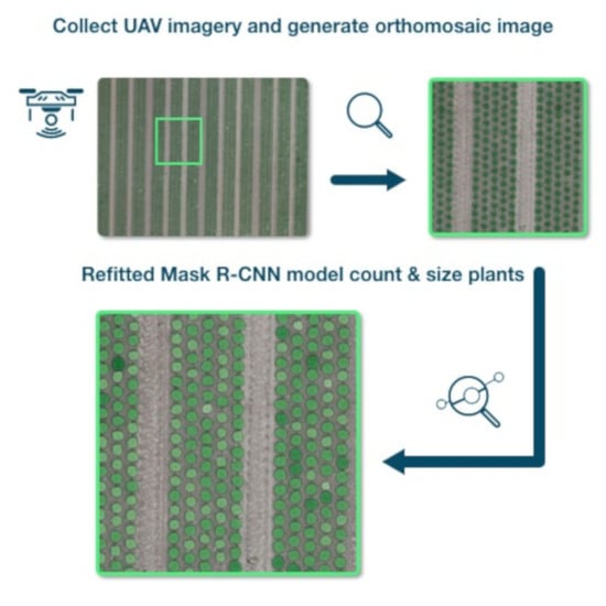
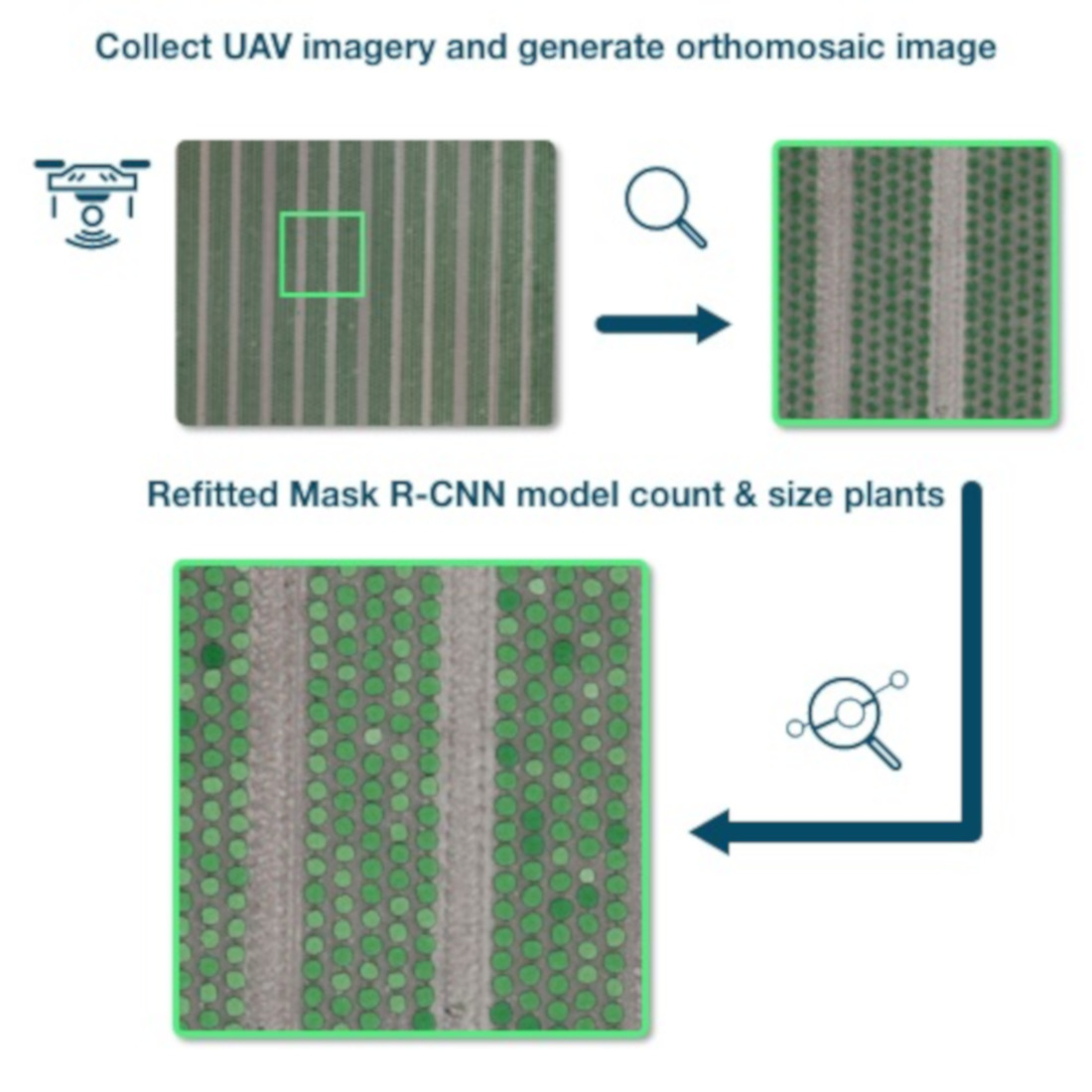
:This work introduces a method that combines remote sensing and deep learning into a framework that is tailored for accurate, reliable and efficient counting and sizing of plants in aerial images. The investigated task focuses on two low-density crops, potato and lettuce. This double objective of counting and sizing is achieved through the detection and segmentation of individual plants by fine-tuning an existing deep learning architecture called Mask R-CNN. This paper includes a thorough discussion on the optimal parametrisation to adapt the Mask R-CNN architecture to this novel task. As we examine the correlation of the Mask R-CNN performance to the annotation volume and granularity (coarse or refined) of remotely sensed images of plants, we conclude that transfer learning can be effectively used to reduce the required amount of labelled data. Indeed, a previously trained Mask R-CNN on a low-density crop can improve performances after training on new crops. Once trained for a given crop, the Mask R-CNN solution is shown to outperform a manually-tuned computer vision algorithm. Model performances are assessed using intuitive metrics such as Mean Average Precision (mAP) from Intersection over Union (IoU) of the masks for individual plant segmentation and Multiple Object Tracking Accuracy (MOTA) for detection. The presented model reaches an mAP of for potato plants and for lettuces for the individual plant segmentation task. In detection, we obtain a MOTA of for potato plants and for lettuces.
1. Introduction
Despite the widely accepted importance of agriculture as one of the main human endeavours related to sustainability, environment and food supply, it is only recently that many data science use cases to agricultural lands have been unlocked by engineering innovations (e.g., variable rate sprayers) [1,2]. Two research domains are heavily contributing to this agriculture paradigm shift: remote sensing and artificial intelligence. Remote sensing allows the agricultural community to inspect large land parcels using elaborate instruments such as high-resolution visible cameras, multi-spectral and hyper-spectral cameras, thermal instruments, or LiDAR. On the other hand, artificial intelligence induces informed management decisions by extracting appropriate farm analytics in a fine-grained scale.
In the research frontline of the remote sensing/artificial intelligence intersection lies the accurate, reliable and computationally efficient extraction of plant-level analytics, i.e., analytics that are estimated for each and every individual plant of a field [3]. Individual plant management instead of generalised decisions could lead to major cost savings and reduced environmental impact for low density crops, such as potatoes, lettuces, or sugar beets, in a similar manner as localised herbicide spraying has been demonstrated to be beneficial [4,5]. For example, by identifying each and every potato, farm managers could estimate the emergence rate (the percentage of seeded potatoes that emerged), target the watering strategy to the crop and predict the yield, while the counting and sizing of lettuces determine the harvest and optimise the logistics.
The resolution required for individual plant detection and segmentation (on the order of 1–2 cm per pixel) imposes a strict limitation in the operations. Fields may be several hundreds of hectares, which implies that the acquired image would be of a particularly large size. In this work, an image with a 2 cm resolution per pixel would generate around gigabytes per hectare. Therefore, UAV imagery for a single field can reach several tens of thousands of pixel of width and height. Any pixel-level algorithms, such as the one required for plant counting and sizing, would need to be (not only accurate but also) computationally efficient. Additionally, the adopted algorithm should be able to exhibit a near-to-optimal performance without requiring a large volume of labelled data. This constraint becomes particularly important since (a) segmentation annotations, like the ones required for individual plant identification, are typically time-consuming and costly and (b) this type of data exhibits a large variance in appearance, both due to inherent reasons (e.g., different varieties and soil types) and due to acquisition parameters (e.g., illumination, shadows). As a matter of fact, opposite to large-volume natural scene images, which are abundant and rather easy to find (e.g., [6]), UAV imagery datasets with segmentation groundtruth typically contain imagery from a unique location covering only a small area. More specifically, as far as we are aware, no large-volume plant segmentation dataset is currently available.
1.1. Recent Progress on Instance Segmentation and Instantiation
The recent proliferation of deep learning architectures [7,8,9], exhibiting unprecedented accuracy in a large spectrum of computer vision applications, has triggered the development of a number of variations on a basic theme, most of them focusing on specific challenging problems, which were beyond the reach of the state-of-the-art for decades. The plasticity of deep learning allowed the emergence of new solutions by linking multiple networks in more complex architectures, or even by adding or removing a few layers from a well-known model. The latter was the case in Fully Convolutional Networks (FCN) [10], which derive from models developed for classification purposes, by simply removing the last layer (used for classification), thus causing the network to learn feature maps instead of classes. This paradigm has been extensively used for binary segmentation applications, in which the model learns pixel-level masks (e.g., in our application, 0 corresponding to ”not a plant” class, and ”1” to ”plant” class). Since a FCN can theoretically be produced from almost any Convolutional Neural Network (CNN) [7], many of the architectures typically used for classification has found a variant used for segmentation, such as AlexNet [7], VGG-16 [8], and GoogLeNet [9], or the most recent Inception-v4 [11] and ResNeXt [12].
A main issue with such simple solutions is that, since the spatial size of the final layer is generally reduced compared to the initial input size due to pooling operations within the network, the learned mask is a super-pixel one, i.e., a mask in which several pixels have been aggregated into one value. In order to recover the initial input spatial size, it has been suggested to combine early high-resolution feature maps with skip connections and upsampling [13]. In another line of research, Yu et al. [14] and Chen et al. [15] both propose to use a FCN supported by dilations (or dilated convolutions) to execute the necessary increase of receptive field. FCN used as an encoder and a symmetrical network used as a decoder characterize Segnet [16] and Unet [17] architectures, which achieve state-of-the-art performances in semantic segmentation.
In theory, a network achieving perfect accurate semantic segmentation could be straightforwardly used for instantiation (i.e., counting of blobs of one of the classes), which is merely needed is to count the connected components. However, in practice, this is a sub-optimal approach, since a model trained for segmentation would not discriminate between a false positive that erroneously joints two blobs (or a false negative that erroneously splits one blob) and a false positive (or negative) with no effect on the instantiation result. Hence, a number of deep learning techniques has been suggested to overcome this obstacle, by achieving simultaneously both semantic segmentation and instantiation. Two of the most well-known are YOLO [18,19,20] and Mask R-CNN [21]. The main difference between the two is that, while YOLO only estimates a bounding box of each instance (blob), Mask R-CNN goes further, by predicting an exact mask within the bounding box.
Mask R-CNN is the latest ”product” of a series of deep learning algorithms developed to achieve object instantiation in images. The first version is R-CNN [22], which was introduced in 2014 as a four-step object instantiation algorithm. The first step of this algorithm consists of a selective search which finds a fixed number of candidate regions (around 2000 per image) possibly containing objects of interest. Next, the AlexNet model [7] is applied to assess if the region is valid, before using a SVM to classify the objects to the set of valid classes. A linear regression concludes the framework to obtain tighter boxes coordinates, wrapping up the bounding box closer onto the object. R-CNN achieved a good accuracy, but the elaborate architecture caused a series of issues, mainly, a very high computational cost. Fast R-CNN [23], followed by Faster R-CNN [24], gradually overcame this limitation by turning it into an end-to-end fully trainable architecture, combining models and replacing the slow candidate selection step. Despite the progress, these R-CNN variations were limited on estimating object bounding boxes, i.e., they did not perform pixel-wise segmentation. Mask R-CNN [21] accomplishes this task by adding a FCN branch to the Faster R-CNN architecture, which predicts a segmentation mask of each object. As a result, the classification and the segmentation parts of the algorithm are independently executed; hence, the competition between classes does not influence the mask retrieval stage. Another important contribution of Mask R-CNN is the improvement of pixel accuracy by refining the necessary pooling operations obtained by bilinear interpolation (instead of rounding operation) with the so-called ROIAlign algorithm.
1.2. Plant Counting, Detection and Sizing
Most of the existing ”plant counting” (i.e., object instantiation in this particular application) techniques of the literature are following a regression rationale. Typically, the full UAV image is split into small tiles, before a model estimates the number of plants in the tile. Finally, the tiles are stitched and the total number of plants, as well as some localisation information, is returned.
For example, in Ribera et al. [25], the authors train an Inception-V3 CNN model on frames of perfectly row-planted maize plants to perform a direct estimation of the number of plants. On the other hand, both Aich et al. [26] and Li et al. [27] suggest a two-step regression approach (with randomly-drilled crops, respectively wheat and potato). In both of these works, initially, a segmentation mask of the plants is derived, either by training a Segnet model [26] or by simply (Otsu) thresholding a relevant vegetation index [27]. Next, a regression model is run, a CNN in [26] and a Random Forest in [27].
This two step-approach is also used in other works, e.g., [28] for Sorghum heads, which have the advantage of presenting well separated red-orange rounded shapes, [29] for denser crop stages and [30] for tomato fruits, the two last ones, though, using in field, and not remote sensing imagery. One of the weaknesses of such algorithms is that they do not consider the possibility of a plant split between two successive tiles, leading to being falsely counted twice. An interesting solution to overcome this issue was proposed in [3] and in [31] (improving [29]), who employ a network which additionally predicts a density map of the center of the plants for the entire input image.
In general, methods exploiting regression additionally provide at least some localisation information. In order to improve the accuracy, as well as to achieve an easier to be visually evaluated instantiation, several authors have suggested the estimation of the center of the plants. e.g., Pidhirniak et al. [32] propose a solution to palm tree counting with a U-Net [17] predicting a density map of the center of the plants completed by a blob detector to extract the geo-centers. A similar method is considered in [33]. In this work, a segmentation by thresholding on a vegetation index is carried out, before implementing a Watershed algorithm to extract vegetation at a sub-pixel level. Subsequently, a CNN is trained to predict pixels corresponding to the center of these plants and a post-processing step concludes the pipeline to remove outliers. A similar approach has also been developed to detect corn plants in [34] and in [35]. Kitano et al. [34] firstly use Unet [17] for segmentation and then morphological operations for detection. Kitano et al. [34] benefit from significantly higher resolution than in [35], for reference, which may lead to scalability issues when having to fly a UAV over hundreds of hectares of land. García-Martínez et al. [35] use normalized cross-correlation of samples of thresholded vegetation index map, which may introduce false positives in the presence of weeds. Malambo et al. [36] demonstrate similar work on sorghum heads detection and [37] with cotton buddings, two small rounded shaped plants. Firstly, for the segmentation task, [36] train a Segnet [16] while [37] use a Support Vector Machine model coupled with morphological operations for detection, following the approach of Kitano et al. [34].
Finally, in [38], in [39] and in [40], three methods are introduced which are closer to the context of our paper. In [38], a YOLO model is used to perform palm tree counting and bounding-box instantiation. In [39], a RetinaNet [41] is used in a weakly supervised learning model aiming at annotating a small sample of sorghum heads imagery. In [40], the authors customize a U-Net model to generate two outputs, a field of vectors pointing to the nearest object centroid and a segmentation map. A voting process estimates the plants, while also producing a binary mask, similarly to our output. Oh et al. [42] achieve the task of individual sorghum heads segmentation. Detection models for plant counting have also flourished in late 2019, with the democratization of Faster R-CNN [24]. The precursor of Mask R-CNN has been adopted in works such as in [43] for banana plant detection with three different sets of imagery at different resolutions, of which one at a similar resolution to the dataset proposed in this paper. Collecting UAV data at three different flight heights enable them to triple their dataset capacity by reusing annotations. Liu et al. [44] also benefit from Faster R-CNN [24] using high resolution maize tassels imagery from only one field and one date of acquisition, which limits the variability of encountered growth stages. In the works of [45,46], they rely on Faster R-CNN for detecting plants and [47] use Mask R-CNN for individual segmentation of oranges.
1.3. Aim of the Study
Based on the above rationale, the backbone of the selected method for achieving a fully practical and reliable individual plant segmentation and detection is an algorithm which exhibits state-of-the-art accuracy, is computationally fast during inference, and exhibits a good performance when applying transfer learning from a pre-trained model on natural scene images to a rather small domain dataset. A proposed method, which combines all of the desired characteristics, is the so-called Mask R-CNN. This architecture is suggested to be used for this task, after of course adjusting it to the ad-hoc characteristics of this particularly challenging setup. Apart from being one of the first end-to-end remotely sensed individual plant segmentation and detection methods in the literature, the main contributions of this work are (a) the adjustment of Mask R-CNN to individual plant segmentation and detection for plant sizing (b) the thorough analysis and evaluation of transfer learning in this setup, (c) the experimental evaluation of this method on datasets from multiple crops and multiple geographies, which generate statistically significant results, and (d) the comparison of the data-driven models derived with a computer vision baseline for plant detection.
The rest of this paper is organized as follows. In Section 2 Material and Methods, at first, the datasets created are detailed. Then, the Mask R-CNN architecture is discussed with a great level of detail in conjunction with an open source implementation to adapt the complex parametrization of this framework to the plant sizing problem. Subsequently, the transfer learning strategy adopted for training this network on this specific task is presented before explaining the hyperparameters’ selection strategy. To follow, a computer vision baseline algorithm for plant detection is presented. At last, all the metrics used for the experimental evaluation of this approach are described. Section 3 presents the obtained results followed by discussion in Section 4. Section 5 concludes this work.
2. Materials and Methods
2.1. Datasets
2.1.1. Study Area
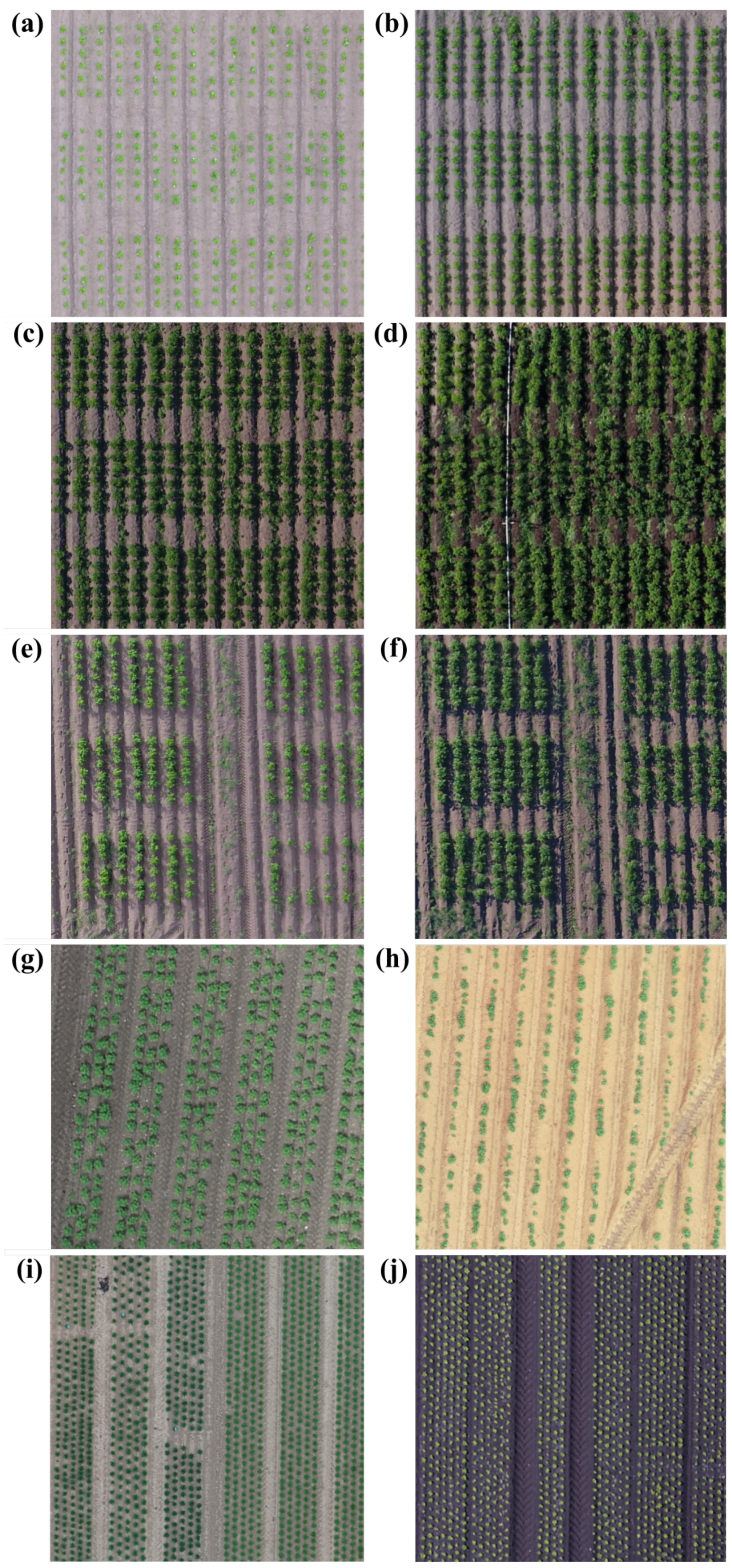
UAV RGB imagery has been acquired over three different potato UK fields (P1, P2, P3), one Australian field (P4), and two different UK lettuce fields (L1, L2). Table 1 summarizes the information related to the acquisition of the imagery fore each field. The acquisition was planned in order to cover the full span of growth stages from emergence (plant size of more than 8 cm) to the point where the canopy closes. This translates into a time window for the UAV flights from 4 to 7 weeks after emergence. Having imagery over several dates allows for corregistering our imagery and reuse annotations for all images, making the data annotation process more efficient while capturing data at different growth stages. The imagery for lettuce plants only includes two acquisition dates for two different fields. However, the lettuce fields present a wider range of growth stages, compensating for the reduced number of flight dates and increasing the variety in growth stages in the dataset. Imagery acquisition is carried out on diffuse light days two hours before or after solar noon to avoid shadows and hot-spots. UAV photographs are then stitched up together into a unique orthomosaic image using a Structure-from-Motion algorithm. The annotation process will be considerably facilitated by the use of orthomosaic images. From these images, image tiles are generated with a size of pixels to be fed into the model. RGB UAV images of potato plants and lettuce plants have been acquired with a resolution between cm and cm per pixel. At such resolutions, the canopy size and shape can be correctly identified with enough discrete pixels from the soil and vegetation classes. The fields are composed of sandy or silty soils which look similar in UAV RGB imagery. Figure 1 shows a sample from each orthomosaic image included in our datasets.
2.1.2. Datasets’ Specifications
The COCO dataset features a large-scale object instance segmentation dataset with million objects over 200 K images across 80 object categories. Imagery covers natural scenes including many different objects. Therefore, not all of the objects are labeled and the groundtruth segmentation can be coarse.
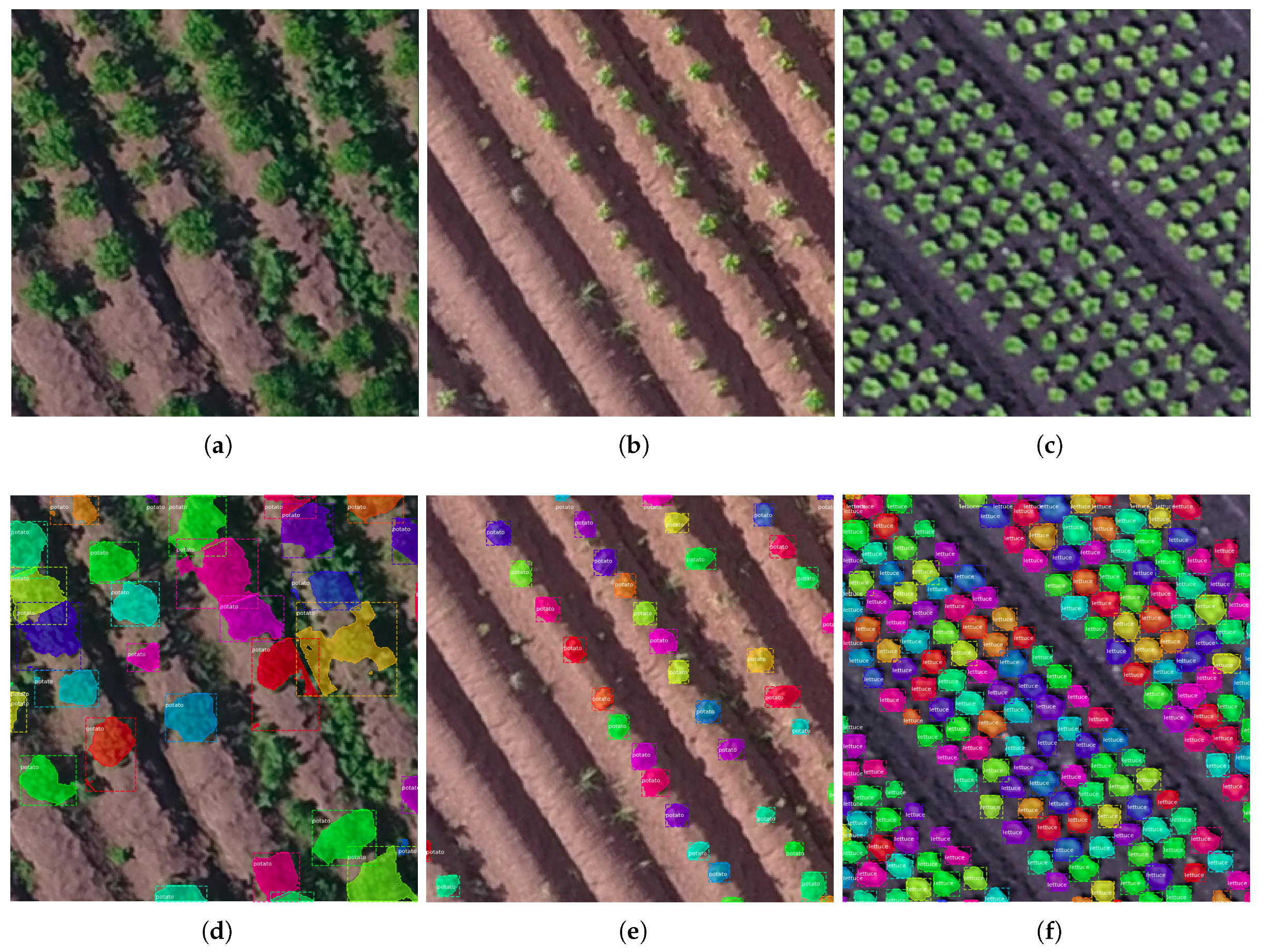
In-house task-related datasets have been created thanks to the imagery acquired in the study area, and Table 2 provides details with the following naming conventions: C for “Coarse”, R for “Refined”, Tr for “Training”, and Te for “Test”. POT_CTr, is a coarsely annotated dataset of 340 images of potato plants. Annotation work was completed by copying bounding boxes of the same size over the most merged surveys and these boxes were manually, but coarsely, adjusted. The mask was obtained by applying an Otsu threshold [27] to separate soil and vegetation within each bounding box. Growth stages selected enabled the human annotator to visually separate plants with bounding box delimitation and allowing for a small overlap for the coarse dataset. Consequently, this semi-automatic labelling displays imprecision in the groundtruthing as shown in Figure 2d. POT_CTr was used as a proof of concept that fine-tuning Mask-R-CNN with small and coarse datasets could lead to satisfactory results. However, metric results could not be trusted considering the quality of the annotation. As opposed to, POT_RTr is a training set carefully annotated at a pixel level covering sampled patches from the same fields from the UK and containing an extra field from Australia. It brings variability in the size of plants, variety and type of soils. POT_RTe presents the same characteristics and it was kept exclusively as a test set to compare all models presented. Finally, LET_RTr is also a training set accurately annotated with lettuce plants in imagery acquired in the UK. LET_RTe is the corresponding test set. Figure 2 displays samples from all these datasets. As specified in Section 1.2, [47] achieved state-of-the art accuracy training Mask R-CNN on RGB in-field images of oranges with a dataset size of 150 images of and a total of 60 instances which is smaller than what our datasets look like.
2.2. Mask R-CNN Refitting Strategy
The deep learning model introduced to tackle the plant counting and sizing tasks is based on the Mask R-CNN architecture, which is adjusted for this problem. As a matter of fact, if the original model (i.e., the one trained on a large number of natural scene images with coarsely-annotated natural scenes objects) is trained or applied for inference without modifications of the default parameters on UAV images of plants, the results are particularly poor. The main reason behind this failure is the large number of free parameters (around 40) in the Mask R-CNN algorithm. This section reviews thoroughly the Mask R-CNN’s architecture and evaluates how each parameter may affect performances. By following the Matterport’s implementation [48] terminology and architecture, the goal is to unfold the parameters’ tuning process followed in this paper to ensure a fast and accurate individual plant segmentation and detection output while facilitating reproducibility. This approach sets up a bridge of knowledge between the theoretical description of this network and the operational implementation on a specific task. Subsequently, strategies of transfer learning which obtain state-of-the-art results with the Mask R-CNN based architecture on the panel of datasets explored are described. To conclude this section, a description of a computer vision baseline targeting the plant detection task is presented.
2.2.1. Architectural Design and Parameters
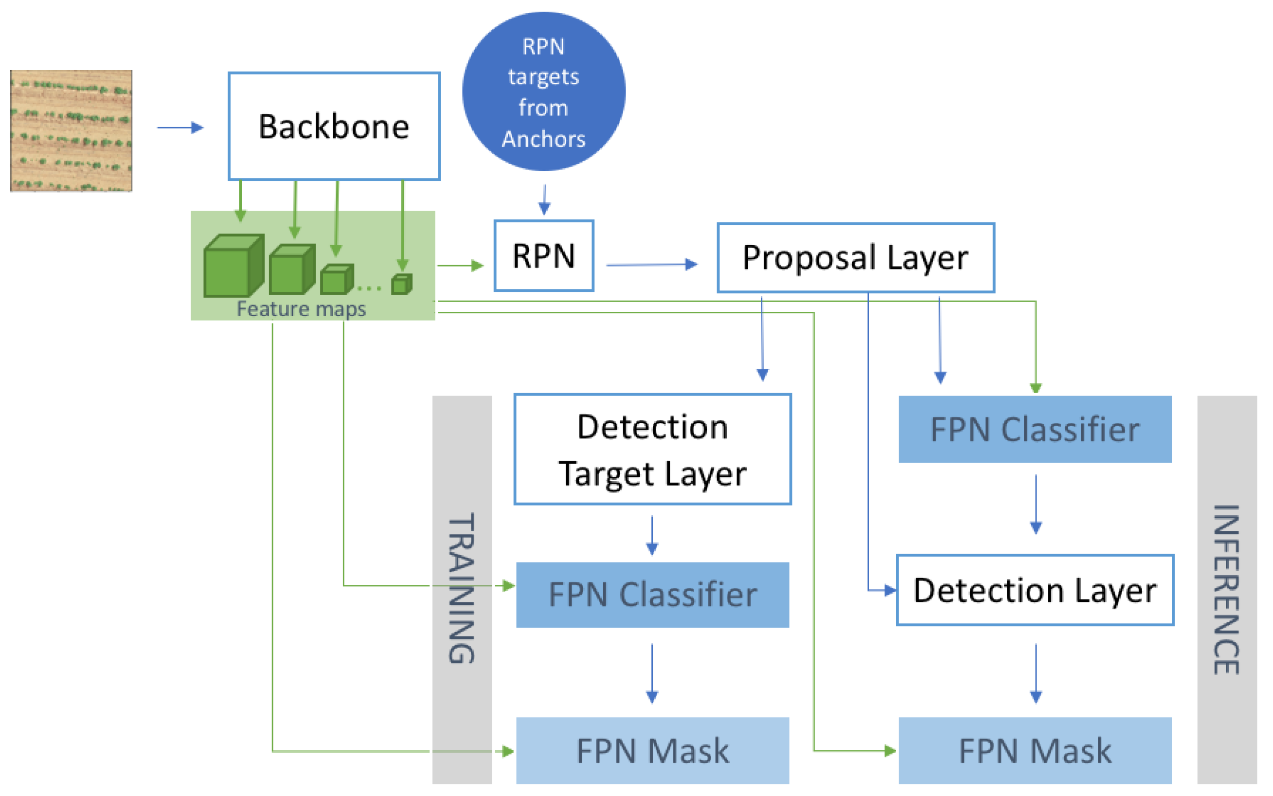
The use of Mask R-CNN in the examined setup presents several challenges, related to the special characteristics of high-resolution remote sensing images of agriculture fields. Firstly, most of the fields have a single crop, the classification branch of the pipeline is a binary classification algorithm, a parameter which affects the employed loss function. Secondly, the remotely sensed images of plants impose the target objects (i.e., plants) to not present the same features, scales, and spatial distribution as natural scene objects (e.g., humans, cars) included in the COCO datasets used for the original Mask R-CNN model training. Thirdly, the main challenges of this setup are different than many natural scene ones. For example, false positives due to cluttered background (a main source of concern in multiple computer vision detection algorithms) is expected to be rather rare in plant counting/sizing setup, while object shadows affect the accuracy than in several computer vision applications much more. Due to these differences, Mask R-CNN parameters need to be carefully fine-tuned to achieve an optimal performance. In the following sub-sections, we analyse this fine-tuning, which, in some cases, is directly linked to the ad-hoc nature of the setup and in others is the result of a meticulous trial-and-error process. Figure 3 describes the different blocks composing the Mask R-CNN model and Table A1, in Appendix A, associates acronyms representing the examined model free parameters with the variable names used in Matterport’s implementation [48] for reproducibility.
2.2.2. Backbone and RPN Frameworks
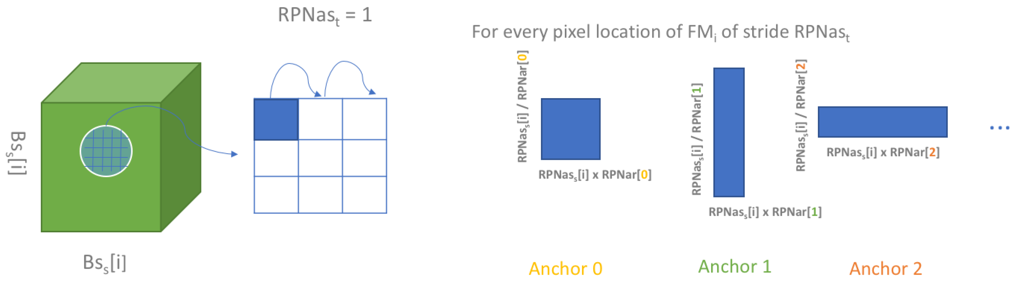
The input RGB image is fed into the Backbone network in charge of visual feature extraction at different scales. This Backbone is a pre-trained ResNet-101 [49] (in our study). Each block in the ResNet architecture outputs a feature map and the resulting collection is served as an input to different blocks of the architecture: the Region Proposal Network (RPN) but also Feature Pyramid Network (FPN). By setting the backbone strides , we can choose the sizes of the feature maps which feed into the RPN, as the stride controls downscaling between layers within the backbone. The importance of this parameter lies in the role of the RPN. For example, induces (all units in pixels) if the input image size is squared of width 256 pixels. The RPN targets generated from a collection of anchor boxes form an extra input for the RPN. These predetermined boxes are designed for each feature map with base scales linked to the feature map shapes , and a collection of ratio is applied to these . Finally, anchors are generated at each pixel of each feature map with a stride of . Figure 4 explains the generation of anchors for one feature map. In total, with the number of RPN anchors ratios introduced, , the total number of anchors generated is defined as
All the coordinates are computed in the original input image pixel coordinates system. All of the anchors do not contain an object of interest, implying that anchors matching the most with the groundtruth bounding boxes filters will be selected. This matching process is carried out by computing the Intersection Over Union (IoU) between anchor boxes and groundtruth bounding boxes locations. If , then the anchor is classified as positive, if as neutral and finally if as negative. Then, the collection is resampled to ensure that the number of positive and negative anchors is greater than half of , which is a share of the total anchors kept to train the RPN. Eventually, the RPN targets have two components for each image: a vector which states if each of the anchors is positive, neutral or negative, and the second component is represented by delta coordinates between groundtruth boxes and positive anchors among the selected anchors to train the RPN. It is essential to note that only groundtruth instances are kept per image to avoid training on images with too many objects to detect. This parameter is important for training on natural scene images composing the COCO dataset as they might contain an overwhelming number of overlapping objects. Dimension of the targets for one image are and , where and are the normalised distance of the coordinates centers between groundtruth and anchor boxes, whereas and respectively deal with the logarithm delta between height and width. Finally, the RPN is a FCN aiming at predicting these targets.
2.2.3. Proposal Layer
The Proposal Layer is plugged onto the RPN and does not consist of a network but of a filtering block which only keeps relevant suggestions from the RPN. As stated in the previous section, the RPN produces scores for each of the anchors with the probability to be characterised as positive, neutral or negative and the Proposal Layer begins by keeping the highest scores to select the best anchors. Predicted delta coordinates from the RPN are coupled to the selected anchors. Then, the Non-Maximum Suppression (PNMS) algorithm [50] is carried out to prune away predicted RPN boxes overlapping with each other. If two boxes among the have more than overlap, the box with the lowest score is discarded. Finally, the top for training phase and for inference phase are kept based on their RPN score.
At this stage, the training and inference paths begin to be separated despite the inference path relyinng on blocks previously trained.
2.2.4. Detection Target Layer
As seen in Figure 3, the training path after the Proposal Layer begins with the Detection Target Layer. This layer is not a network but yet another filtering step of the Regions of Interest (ROIs) outputted by the Proposal Layer. However, this layer uses the groundtruth boxes to compute the overlap with the ROIs and set them as a boolean based on the condition . Finally, these ROIs are subsampled to a collection of ROIs but randomly resampled to ensure a ratio of the total as positive ROIs. As the link with groundtruth boxes is established in this block and the notion of anchors is dropped, the output of this Detection Target Layer is composed of ROIs with corresponding groundtruth masks, instance classes, and delta with groundtruth boxes for positive ROIs. The groundtruth boxes are padded with 0 values for the elements corresponding to negative ROIs. These generated groundtruth features corresponding to the introduced ROIs features will serve as groundtruth to train the FPN.
2.2.5. Feature Pyramid Network
The Feature Pyramid Network (FPN) is composed of the Classifier and by the Mask Graph. The input to these layers will be referred to as Area of Interest AOIs, as they are essentially a collection of regions with their corresponding pixel coordinates. The nature of these AOI can vary during the training and inference phase as shown in Figure 3. Both of the extensions of the FPN (Classifier and Mask) present the same succession of blocks, composed of a sequence of ROIAlign and convolution layers with varying goals. The ROIAlign algorithm, as stated in the beginning of this section, has to pool all feature maps from FPN lying within the AOIs by discretising them into a set of fixed square pooled size bins without generating a pixel misalignment unlike traditional pooling operations. After ROIAlign is applied, the input of the convolution layers is a collection of same size squared feature maps, and the size of the batch is the number of AOIs. In the case of the Classifier, the output of these deep layers is composed of a classifier head with logits and probabilities for each item of the collection to be an object and belong to a certain class as well as refined box coordinates which should be as close as possible from the groundtruth boxes used at this step. In the case of the Mask graph, the output of this step is a collection of masks of fixed squared size which will later on be re-sized to the shape in pixels of the corresponding bounding box extracted in the classifier.
In the previous Section 2.2.4, it has been explained that, for the training phase, the Detection Layer Target outputs AOIs and computes corresponding groundtruth boxes, class instances, and masks which are used for the training of a sequence of FPN Classifier and Mask Graph as shown in Figure 3. For the inference path, the trained FPN is used in prediction, but the FPN Classifier is firstly applied to the AOIs extracted from the Proposal Layer, followed by a Detection Layer, as detailed in the following Section 2.2.6. It ensures the optimal choice of AOIs to only keep AOIs. Finally, these masks are extracted by the final FPN Mask Graph in prediction mode.
2.2.6. Detection Layer
This block is dedicated to filtering the proposals coming out from the Proposal Layer based on probability scores per image per class extracted from the FPN Classifier Graph in inference mode. AOIs with low probability scores under are discarded, and NMS is applied to remove lowest score AOI overlapping more than with a higher score. Finally, only the best AOIs are selected to extract their masks with the following block FPN Mask Graph.
Each of these blocks is trained with a respective loss in regard to the nature of its function. Boxes’ coordinates prediction is associated with a smooth L1-loss, binary mask segmentation with binary cross-entropy loss, and instance classification with categorical cross-entropy loss. The Adam optimiser [51] is used to minimize these loss functions.
2.2.7. Transfer Learning Strategy
Transfer learning describes the process of using a model pretrained for a specific task and retraining this model for a new task [52]. The benefits of this process are to improve training time and performance due to previous domain knowledge demonstrated by the chosen model. Transfer learning can only be successful if the features learnt from the first model are general enough to envelope the targeted domain of the new task [53].
Deep supervised learning methods require a large amount of annotated data to produce the best results possible, especially with large architecture with several millions of parameters to learn such as Mask R-CNN. Therefore, the necessary dataset size is the main factor for a successful model achieving state-of-the-art instance segmentation. Zlateski et al. [54] advocate for 10 K images per class accurately labeled to obtain satisfying results on instance segmentation tasks with natural scene images. At a resolution between cm and 2 cm, digitising 150 masks of a low density crop takes around an hour for a trained annotator. As a result, precise pixel labeling of 10 K images implies a significant amount of person-hour. However, Zlateski et al. [54] prove that pre-training CNN on a large coarsely-annotated dataset, such as the COCO dataset (200 K labeled images) [6] for natural scene images, and fine-tuning on a smaller refined dataset of the same nature leads to better performances than training directly on a larger finely-annotated dataset. Consequently, transferring the learning from the large and coarse COCO dataset to coarse and refined smaller plant datasets makes the complex Mask R-CNN architecture portable to the new plant population task.
2.2.8. Hyper Parameters Selection
The parametrization setup of the Mask R-CNN model is key to facilitating the training of the model and maximizing the number of correctly detected plants. It was observed that the default parameters in the original implementation of [48] would lead to poor results due to an excessive amount of false negatives. Therefore, an extensive manual search guided by the the understanding the complex parameterization process of Mask R-CNN detailed in Section 2.2.1. Mask R-CNN is originally trained on the COCO dataset which is composed of objects of highly varying scales that can sometimes fully overlap between each other (leading to the presence of the so-called crowd boxes). In consideration of the datasets presented in our study, most of the objects of interest have a smaller range of scales, and two plants cannot have fully overlapping bounding boxes. Regarding the scale of both potato and lettuce crops, an individual plant goes from 4 to 64 pixels at our selected resolutions. Based on these observations, optimising the selection of the regions of interest through the RPN and the Proposal Layer can be solved by tuning the size of the feature maps and the scale of the anchors . cannot be modified due to the Backbone being pre-trained on COCO weights and the corresponding layers frozen. Then, following the explanation in Section 2.2.2, the pixel size of was chosen to include sizes of feature maps corresponding to the range of scales of the plant “objects”. In addition, taking into account the imagery resolution (see Section 2.1.2) and an estimation of the range of the plant drilling distance, can easily be inferred. We estimated that not more than potatoes and lettuces could be found in an image of pixels. This observation also allows for setting the number of anchors per image to train the RPN and the number of in the Detection Target layer to be set to the same value. Starting from this known estimation of the maximum number of expected plants, this bottom-up view of the architecture is key to finding a more accurate number of AOIs to keep at each block and phase for each of the crops investigated. The parameters involved are and . Manual variations of these parameters by step of 100 have been attempted. Thresholds used for IoU in the NMS (, ) and confidence scores () can also be tuned but the default values were kept due to our tuning attempts being inconclusive.
2.3. Computer Vision Baseline
A computer vision baseline for plant detection is considered to compare predicted plant centers by the Mask R-CNN model. As a starting point of this method, the RGB imagery acquired by UAV has to be transformed to highlight the location of the center of the plants. Computing vegetation indexes to highlight image properties is a mastered strategy in the field of remote sensing. Each vegetation index presents their own strengths and weaknesses as detailed in Hamuda et al. [55]. The Colour Index of Vegetation Extraction (CIVE) [56] is presented as a robust vegetation index dedicated to green plant extraction in RGB imagery and defined as
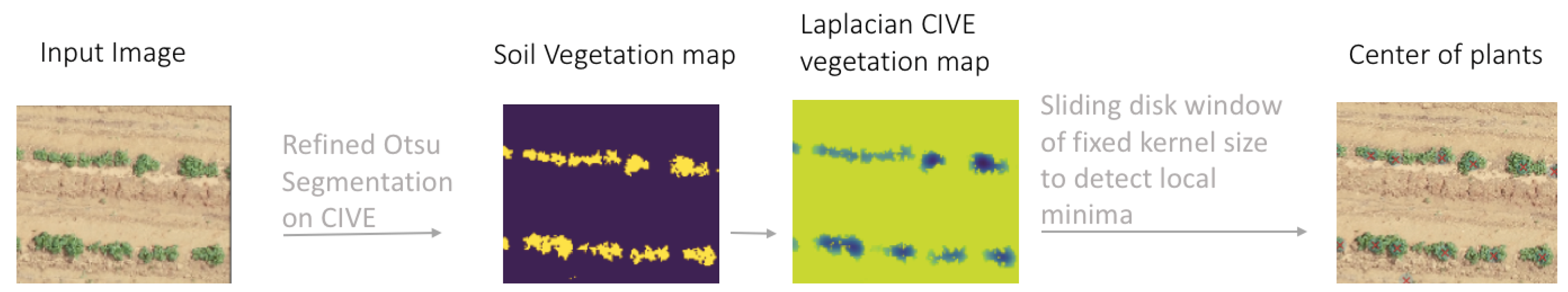
where R, G and B respectively stand for red, green and blue channels defined between 0 and 255. In order to have a normalised index, all channels are individually divided by 255. Segregating between vegetation and soil pixels in an automated manner is possible using an adaptive threshold such as the Otsu method [27]. In this classification approach, foreground and background pixels are extracted by finding the threshold value which minimizes the intra-class intensity variance. By applying Otsu thresholding on CIVE vegetation index, a binary soil vegetation map is obtained, unaltered by highly varying conditions of illumination and shadowing. The Laplacian filtered CIVE map with masked soil pixels () highlights regions of rapid intensity change. Potato plants and lettuce plants pixels of this map are meant to have minimal change close to their center due to homogeneous and isotropic properties of their visual aspect. Therefore, finding the local minima of the map should output the geolocation of these plant centers. This is why all pixels are tested as geo-centers of a fixed size disk window and are only considered as the center of a plant if their value is the minimum of all pixels located within the window area. This framework is summarized in Figure 5.
2.4. Evaluation Metrics
Metrics dedicated to the evaluation of the performance of algorithms in computer vision are strongly task and data dependent. In this paper, our first interest is to compare different strategies of transfer learning using various datasets adopting a data hungry Mask R-CNN model for the instance segmentation task. A plant is considered as a true positive if the intersection over union of the true mask and a predicted one is over a certain threshold as . Varying this threshold from to with a step scale of with averaging allows the widening of the definition of a detected plant. It defines the mean Average Precision (mAP) such as the average precision for a set of different thresholds.
Detection evaluation differs from the individual segmentation metric as the output of the algorithm is a collection of points. The Multiple Object Tracking Benchmark [57] comes with a measure which covers three error sources: false positives, missed plants, and identity switches. A distance map between predicted and true locations of the plants is computed to determine the possible pairs and derive the number of misses, number of false positives, the number of mismatches, and the number of objects which allows for computing the multiple object tracking accuracy (MOTA)
MOTA metric presents the advantage to synthesize error sources monitoring while the conventional Precision and Recall metrics allow for more straightforward interpretability. With being the number of true positives, Precision and Recall are defined as follows:
3. Results
All models have been trained using an Nvidia GPU TITAN X 12 GB. A GPU with 12 GB of memory that typically allows a maximum batch size of eight images of dimensions. We did not use batch normalization due to performance losses demonstrated on small batches [58].
Live data augmentation was performed on the training images with vertical and horizontal flips to artificially increase the training set size. Training a model without data augmentation can lead to overfitting and trigger an automated early stopping of the training phase.
Datasets used for training phases were split into for training and for validation to evaluate the model at the end of each training epoch.
Hyper parameters for each of the following models have been set in accordance with the method stated in Section 2.2.8. Table 3 states the different settings used for training on each dataset described in Table 2.
3.1. Individual Plant Segmentation with Transfer Learning
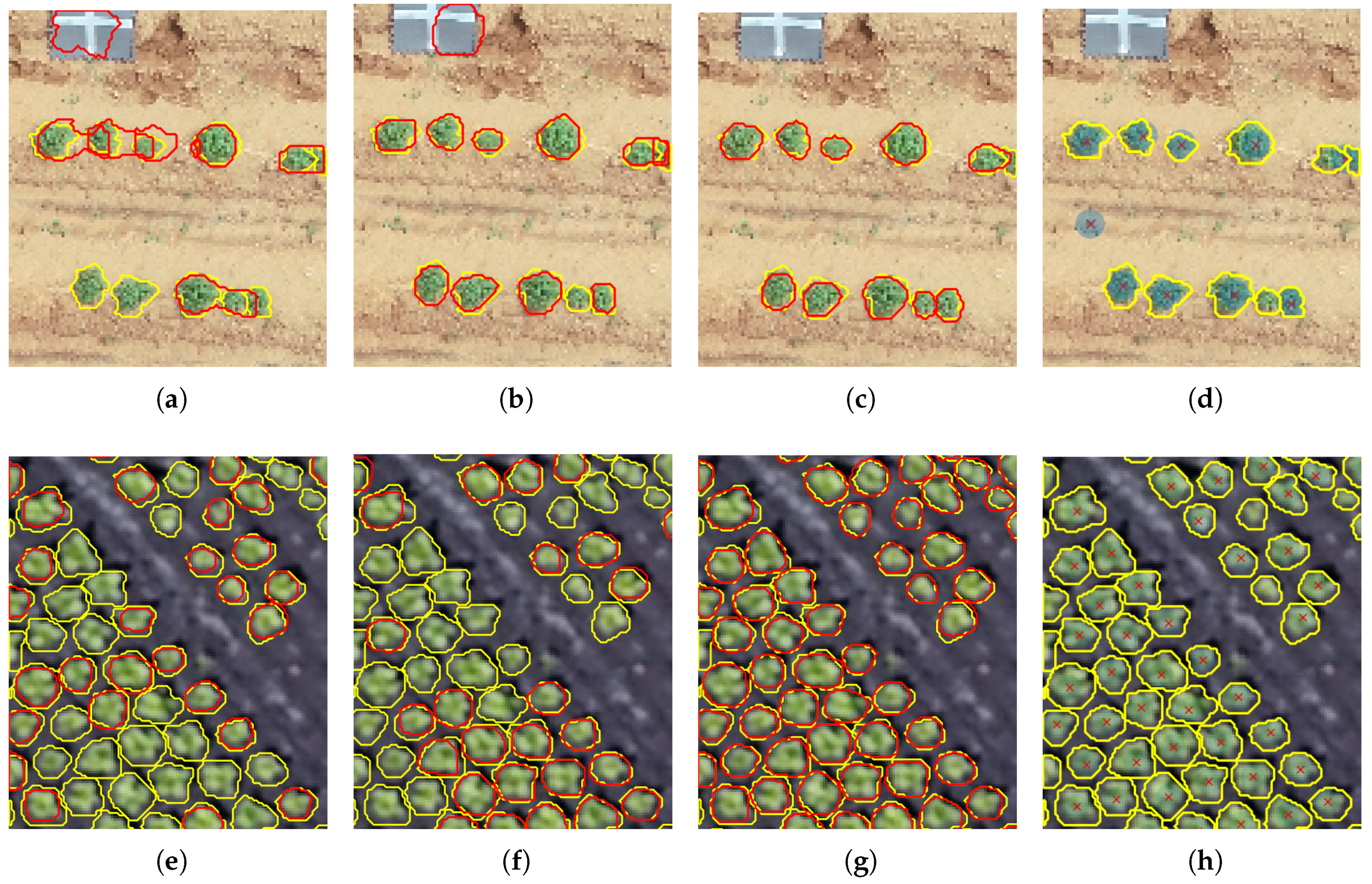
First, we performed transfer learning from the COCO weights (obtained by training the Mask R-CNN with parameters found in Table 3) on the POT_CTr dataset (model M1_POT). Mean Average Precision (mAP) over POT_RTe is which is low, as initially expected, due to the POT_CTr training set being coarsely annotated. We then performed transfer learning from the COCO weights to the POT_RTr dataset and obtained a higher mAP of on the POT_RTe dataset due to the refined annotations of the POT_RTr dataset (model M2_POT). Finally, retraining on POT_RTr dataset from the POT_CTr weights (model M3_POT) led to the best mAP of demonstrating that pre-training a network on a coarsely labeled dataset before fine-tuning on a polished dataset can definitely boost the accuracy of a model. Figure 6a–c respectively show the inference of M1_POT with mAP of , M2_POT with mAP of and M3_POT with mAP of on an image from the POT_RTe dataset. The resulting segmentation and the number of potato plants detected improve significantly as the mAP values are increased. Moreover, the boundaries of the predicted masks drawn on the images fit the contours of the plants better.
In order to assess whether M3_POT, which has been trained on potato plants, presents the same performance on another low density green-colored crop, M3_POT was used in inference on LET_RTe, composed of aerial images containing lettuce plants in fields. A mAP of was calculated and by dissecting the parameters used in Mask R-CNN, this low accuracy score was explained by an excessively small limiting the number of possible lettuce plants which could be found in one image. By raising to 300 as well as the number of ROIs kept after using the NMS in training and inference phases (parameters and ), the likelihood of detecting all lettuce plants is significantly increased. As the number of AOIs to detect is higher, was also increased to obtain more ROIs training the FPN. Consequently, the number of groundtruth objects to consider and the number of predicted objects were also inflated. Following these adjustments, a mAP of for M3_POT used in inference on LET_RTe still proved to be low, implying that the updated training parameters would not make any difference in prediction mode. Therefore, we conclude that a model trained on potato plants transfers poorly to lettuce plants detection and segmentation. Two models based on the COCO weights and M3_POT weights were then trained separately on the LET_RTr dataset. The models (M1_LET and M2_LET) respectively obtained a mAP of and on the LET_RTe dataset. A similar conclusion as for models trained on potato plants can be drawn since pre-training on another crop seems to improve the final model. Figure 6e–g respectively show the inference outputs of M3_POT with mAP of , M1_LET with mAP of , and M2_LET with mAP of on an image from the LET_RTe dataset. The resulting segmentation and the number of potato plants detected greatly improve as the mAP values demonstrate, as well as the boundaries of the predicted masks. Higher values of mAP are observed for lettuce plants than for potato plants. This could imply that the individual plant segmentation task is easier to achieve on the lettuce crop considering the conditions of acquisition of the imagery in both of the datasets, detailed in Section 2.1.
3.2. A Comparison of Computer Vision Baseline and Mask R-CNN Model for Plant Detection
The presented Mask R-CNN model for individual plant segmentation encompasses the fulfillment of the task of detection. The models with highest mAP, respectively M3_POT for potato plants and M2_LET for lettuce plants, have been compared to the Computer Vision based model detailed in Section 2.3. This latest model outputs coordinates corresponding to the center of the plants and postprocessing was also conducted on the masks predicted by the Mask R-CNN based model to calculate the plants’ centroids for comparison. Table 4 displays results for both of the methods applied on the POT_RTe dataset. MOTA, precision, and recall scores are all higher for the Mask R-CNN based model than for the traditional Computer Vision (CV) method. Figure 6c and Figure 6d respectively show the predictions of M3_POT and CV on a sample from POT_RTe. It should be noted that some weeds are wrongly classified as potato plants by the CV method and a higher number plants were missed than with the Mask R-CNN based model. These false negatives can be explained for the CV method by the distance between two local minima of the map being smaller than the size of the chosen window which occurs when plants are very close to each other. It is suggested that a small and isolated plant can be missed due to a possible inaccuracy of the Otsu thresholding or an excessively strong smoothing effect of the Laplacian. However, it shall be noted that the imagery within POT_RTe represents fine farming practices and data collection timing, implying that there is close to no weed in the field and the potato plants’ canopy is not closed. It is thought that M3_POT could have encountered difficulties if any of these two edge cases would have appeared in the data.
The same experiment is repeated to compare the CV method and M2_LET on LET_RTe. Once again, better MOTA values are observed for the Mask R-CNN based model as seen in Table 5. Lettuce plants display the strong advantage of being of a round shape, compact and well-separated from each other. Lettuce is also a high-value crop, meaning that the amount of care per hectare of crop is high and may result in more organised fields with a reduced presence of weeds. These characteristics translate into a more systematic uniqueness of the local minima of the LfC. Consequently, the corresponding center of a lettuce plant is easier to detect than for a potato plant. Indeed, potato plants can present an irregular canopy and, often, merge with other plants. The CV method reaches the high scores of MOTA (), Precision (), and Recall (). The deep learning model also benefits from the advantageous visual features displayed by lettuce plants in comparison with potato plants. A perfect precision score of 100% is reached for the Mask R-CNN refitted model, meaning that no element is wrongly identified as a plant for the entire LET_RTe test set. The model also outperforms the CV method with a MOTA of and a Recall of . A sample extracted from the LET_RTe dataset is processed by M2_LET and illustrated in Figure 6g. It can be observed that only lettuce plants on the edges of the image are missed due to the convolutional structure of the network. In comparison to the CV method, with its results illustrated in Figure 6h, is small lettuces that are missed.
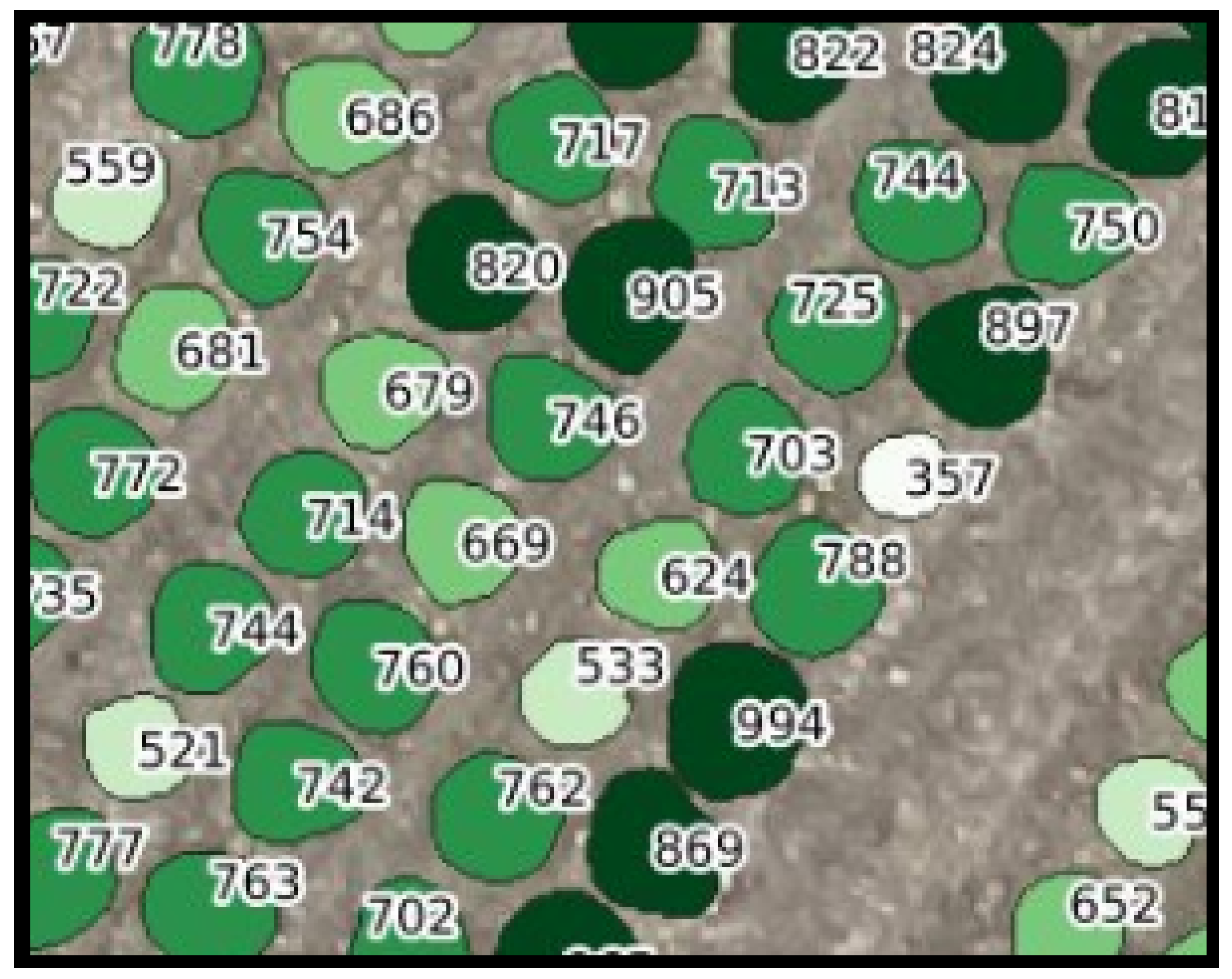
To emphasise the real-world limits of our models, we have converted every pixel mask predicted by and into a square centimetre area using the resolution per pixel. We can observe that the smallest and largest lettuce plants are respectively 122 and 889 , with a mean leaf area of 405 . The smallest and largest potato plants are respectively 40 and 391 , with a mean at 126 . These values inform us that the can detect potato plants as small as 4–5 pixels in diameter in the imagery. Moreover, smaller plants detected by can be interpreted by the fact that potato fields need to be flown early in the season before the plants’ canopy merges. Figure 7 shows a sample image from the L1 field with the predicted masks by . The corresponding size in square centimeter is superimposed over each plant.
4. Discussion
In the existing literature, detailed in Section 1.2, the methodology applied to tackle the plant detection and counting problems often involves a two-step procedure which, firstly, performs segmentation of the vegetation and, secondly, a detection of the plants’ centroids, using either computer vision or deep learning methods [25,26,27,32,33,34,35,36,37]. By relying on the Mask R-CNN architecture, our work presents an all-in-one model allowing to output individual plant masks, aiming at perfecting the complex instance segmentation task and intrinsically leading to outstanding plant detection and counting performances.
In this paper, the focus is both to accurately detect plants to estimate a count per area and to delineate every single plant’s boundaries at pixel-level. In contrast with our work, previous works have adapted regression-based models to predict a count for a given area without any plant location or plant segmentation [25,26,27]. Moreover, we avoid the use of vegetation indices [27,33,35] because (a) the most renowned ones require a multi-spectral camera, which typically has a coarser spatial resolution and is more expensive than an RGB camera and (b) other indices, such as CIVE (Color Index of Vegetation Extraction), are linear combinations of the RGB channels, i.e., learnable from the neural network without explicitly estimating them in a pre-processing stage. Finally, we use an all-in-one model which has already demonstrated its potential in agricultural scenarios using in-field imagery taken from the ground [45,46,47] instead of UAV photographic imagery. By using this unique Mask R-CNN model, we avoid an additional ”patching” step seen in a number of techniques explored in the literature which leads to more complex processing pipelines and performance comparability. [25,26,27,32,33,34,35,36,37].
Previous studies have also developed algorithms aiming at solving individual plant segmentation such as [38] on palm trees and [39] on sorghum heads. However, the imagery resolutions and plant types studied are not comparable with our presented work. Moreover, [38,39,42] solely assess their solutions on the detection task and could not evaluate them on a sizing task due to a lack of accurately-digitized groundtruth mask. Dijkstra et al. [40] propose a method carrying out individual remotely sensed potato plant bounding box detection. This work presents a notable difference with ours as the objective was not to generate accurate masks but exclusively to predict the plants’ centroids within a targeted area associated with each plant. Hence, none of the existing methods enumerated above is directly comparable with our work due to differences in task complexity and metrics being too great.
Bringing together remote sensing and deep learning for plant instance segmentation with the Mask R-CNN embodies a direct automatic cutting-edge approach. Moreover, it outperforms parametrically and a multistep conventional computer vision baseline when used for plant detection. These results were based on the mean Average Precision as a metric for instance segmentation. This metric not only takes into account the matching between the groundtruth masks and their corresponding predictions, but also gradually penalizes the correctness of the resulting mask, at a pixel level, from to of Intersection Over Union. The images collected for our datasets have been manually digitized with a high precision. This allows for assessing the quality of the models’ predictions by comparing with the annotations for each plant. This specific characteristic of our datasets enabled our study to be the first one, to the best of our knowledge, to use mAP using the masks representing plants in UAV images to quantify a model’s performance on a plant sizing task. Ganesh et al. [47] also used Mask R-CNN for in-field orange fruit detection in the trees. However, they don’t evaluate their algorithm for sizing such as we do thanks to the mean Average Precision metric. The MOTA metric, derived from The Multiple Object Tracking Benchmark [57], has recently been introduced in the remote sensing field and represents with fidelity the performance of algorithms developed for object detection. The best model obtained for the potato crop reaches a mAP of , and for the lettuce crop. For plant detection only, these same models respectively obtain a MOTA score of for potato plants and for lettuce plants. In comparison, the traditional computer vision baseline solution tested in this paper only obtains and for the same crops, respectively. Ganesh et al. [47], studying in-field orange fruit detection, obtain a Precision of and a Recall of with their Mask R-CNN model. With our refitted Mask R-CNN models on remotely sensed images, we reach a Precision of (potato plants) and (lettuce plants) and a Recall of (potato plants) and (lettuce plants).
Annotated data in the remote sensing field is a common limitation to projects leveraging the power of deep learning as supervised techniques are data-greedy. The sequential training phases on large natural scenes datasets such as COCO [6], on the coarsely-annotated potato plants dataset and, finally, on the smaller and refined labeled potato plants dataset, allowed to build the best model and highlights a strategy to tackle data scarcity. The resulting model is crop specific despite the fact that potato and lettuce crops are two low-density green-coloured crops. Nonetheless, using the same weights as a basis for a new model for lettuce plant instance segmentation, turns to be a successful strategy. This demonstrates transfer learning capabilities across datasets containing imagery of different plant types. Models yielded poor results when trained on a first specific dataset and used in inference on a second one with other types of objects. This justifies the necessity of understanding the complex parameterization process of Mask R-CNN and this study is the first one, to the best of our knowledge, which disseminates in detail the nodes and effects of this complex model. It also facilitates reproducibility by using the notations of variable names used in an open-source implementation [48].
Our Mask R-CNN based model is robust as it is able to accurately detect and segment plants affected by shadowing effects, occluded by foliage or some degree of overlap between plants. Limitations occur once plants reach a greater merging state but humans annotators also encounter difficulties when digitising plant masks from UAV imagery. The computer vision baseline method for detection has shown to be more sensitive to merged plants. Our Mask R-CNN based model is also capable of rightly ignoring weeds which could be mistaken for potato plants. In contrast, the computer vision baseline algorithm frequently generates false positives when encountering weeds or human-made objects.
To apply this deep learning model presented in this paper to a real-world problem, it is important to note that it has only been trained on frames of pixels. Moreover, the individual plant segmentation outputted is over one frame instead of an image sometimes covering hundreds of hectares. We suggest that, in order to process an entire potato or lettuce field, a preprocessing gridding step should be added so that each frame is fed into the model individually. Then, a postprocessing mosaicking step should be used to reconstitute the whole image and display all predictions at once. Due to the model having issues with plants located right on the image border, a sliding window with overlap between two frames could be developed for the preprocessing module. In regard to the postprocessing module, it should include the cropping of the corresponding overlap whilst plants segmented on two frames should be merged as a unique one. Such preprocessing and postprocessing steps would help to validate the model, but also to potentially create systems that automatically count an entire field and possibly assess the maturity of the crops based on their size. The development of such tool could lead to novel field management practices such as variable fertiliser spraying per plant depending on their size or plant growth stage estimation.
5. Conclusions
Combining remote sensing and deep learning for plant counting and sizing using the Mask R-CNN architecture embodies a direct and automatic cutting-edge approach. Moreover, it outperforms the manually-parametrized computer vision baseline requiring multiple processing steps when used for plant detection. This study is the first one, to the best of our knowledge, to evaluate an algorithm of individual instance segmentation on remotely sensed images of plants. The datasets are composed of high quality digitized masks of potato and lettuces. The success of this approach is conditioned by transfer learning strategies and by the correct tuning of the numerous parameters of the Mask R-CNN training process, both detailed in this study. This justifies the necessity of understanding the complex parameterization process of Mask R-CNN and disseminating the implications and effects of this complex model’s parameters for remote sensing applications. It also facilitates reproducibility by using the notations of variable names of the open-source Matterport implementation [48]. The experiment design has been established to account for practical constraints of the remote sensing field for precision agriculture: commercial farming practices represented in the variability of images of the dataset, scalability for operational use of the model, and scarcity of annotated images at a pixel level.
Author Contributions
Conceptualization, M.M. and F.L.; Data curation, F.L. and V.B.; Investigation, M.M.; Methodology, M.M.; Supervision, F.L.; Validation, M.M.; Visualization, M.M.; Writing—original draft, M.M.; Writing—Review and editing, M.M., F.L., A.H., and P.S. All authors have read and agreed to the published version of the manuscript.
Funding
This research received no external funding.
Conflicts of Interest
The authors declare no conflict of interest.
Appendix A

Table A1.
Acronyms correspondence with Matterport implementation [48].
Table A1.
Acronyms correspondence with Matterport implementation [48].
| Acronym | Variable Name in Matterport Implementation [48] | Description |
|---|---|---|
| List of strides in pixels of each convolution layer which generates the feature maps used from the Backbone. | ||
| List of width in pixels of each squared feature map used to feed the RPN obtained from | ||
| List of base width in pixels of each anchor used for each feature map. | ||
| Stride in pixels of the locations of the anchors generated for each feature map. | ||
| List of ratio to apply on each element of aiming at generating non squared anchors (see Figure 4). | ||
| Number of anchors per image selected to train the RPN. | ||
| Number of kept proposals outputted by the RPN based on their RPN scores. | ||
| IoU threshold for stating overlapping RPN predicted boxes. | ||
| Number of ROIs to keep after NMS in the Proposal Layer for the training phase. | ||
| Number of ROIs to keep after NMS in the Proposal Layer for the inference phase. | ||
| Number of groundtruth instances per image kept to train the network. | ||
| Number of ROIs to keep after the Detection Target Layer. | ||
| Ratio of positive ROIs among the . | ||
| Maximal number of instances that the Mask R-CNN is allowed to output per image in the prediction mode. It also corresponds to the number of AOIs outputted by the Detection Layer. | ||
| Minimum FPN Classifier probability for an AOI to be considered as containing an object of interest. | ||
| NMS threshold used in the Detection Layer. |
References
- Kamilaris, A.; Prenafeta-Boldú, F.X. Deep learning in agriculture: A survey. Comput. Electron. Agric. 2018, 147, 70–90. [Google Scholar] [CrossRef] [Green Version]
- Han, S.; Hendrickson, L.; Ni, B. A variable rate application system for sprayers. In Proceedings of the 5th International Conference on Precision Agriculture, Bloomington, MN, USA, 16–19 July 2000; pp. 1–9. [Google Scholar]
- Wu, J.; Yang, G.; Yang, X.; Xu, B.; Han, L.; Zhu, Y. Automatic counting of in situ rice seedlings from UAV images based on a deep fully convolutional neural network. Remote Sens. 2019, 11, 691. [Google Scholar] [CrossRef] [Green Version]
- Melland, A.R.; Silburn, D.M.; McHugh, A.D.; Fillols, E.; Rojas-Ponce, S.; Baillie, C.; Lewis, S. Spot spraying reduces herbicide concentrations in runoff. J. Agric. Food Chem. 2015, 64, 4009–4020. [Google Scholar] [CrossRef]
- Rees, S.; McCarthy, C.; Baillie, C.; Burgos-Artizzu, X.; Dunn, M. Development and evaluation of a prototype precision spot spray system using image analysis to target Guinea Grass in sugarcane. Aust. J. Multi-Discip. Eng. 2011, 8, 97–106. [Google Scholar] [CrossRef]
- Lin, T.; Maire, M.; Belongie, S.J.; Bourdev, L.D.; Girshick, R.B.; Hays, J.; Perona, P.; Ramanan, D.; Dollár, P.; Zitnick, C.L. Microsoft COCO: Common objects in context. In Proceedings of the European Conference on Computer Vision, Zurich, Switzerland, 6–12 September 2014; Springer: Cham, Switzerland, 2014; pp. 740–755. [Google Scholar]
- Krizhevsky, A.; Sutskever, I.; Hinton, G.E. ImageNet classification with deep convolutional neural networks. In Proceedings of the Advances in Neural Information Processing Systems 25, Lake Tahoe, NV, USA, 3–6 December 2012; pp. 1097–1105. [Google Scholar]
- Simonyan, K.; Zisserman, A. Very deep convolutional networks for large-scale image recognition. arXiv 2014, arXiv:1409.1556. [Google Scholar]
- Szegedy, C.; Liu, W.; Jia, Y.; Sermanet, P.; Reed, S.E.; Anguelov, D.; Erhan, D.; Vanhoucke, V.; Rabinovich, A. Going Deeper with Convolutions. In Proceedings of the IEEE Conference on Computer Vision and Pattern Recognition (CVPR), Boston, MA, USA, 7–12 June 2015. [Google Scholar]
- Kemker, R.; Salvaggio, C.; Kanan, C. Algorithms for semantic segmentation of multispectral remote sensing imagery using deep learning. ISPRS J. Photogramm. Remote Sens. 2018, 145, 60–77, J.ISPRSJPRS.2018.04.014. [Google Scholar] [CrossRef] [Green Version]
- Szegedy, C.; Ioffe, S.; Vanhoucke, V. Inception-v4, inception-resNet and the impact of residual connections on learning. arXiv 2016, arXiv:1602.07261. [Google Scholar]
- Xie, S.; Girshick, R.B.; Dollár, P.; Tu, Z.; He, K. Aggregated residual transformations for deep neural networks. In Proceedings of the IEEE Conference on Computer Vision and Pattern Recognition, Honolulu, HI, USA, 21–26 July 2017. [Google Scholar]
- Shelhamer, E.; Long, J.; Darrell, T. Fully Convolutional Networks for Semantic Segmentation. IEEE Trans. Pattern Anal. Mach. Learn. 2017, 39, 640–651. [Google Scholar] [CrossRef]
- Yu, F.; Koltun, V. Multi-dcale context sggregation by filated convolutions. arXiv 2015, arXiv:1511.07122. [Google Scholar]
- Chen, L.; Papandreou, G.; Kokkinos, I.; Murphy, K.; Yuille, A.L. DeepLab: Semantic Image Segmentation with Deep Convolutional Nets, Atrous Convolution, and Fully Connected CRFs. IEEE Trans. Pattern Anal. Mach. Intell. 2017, 40, 834–848. [Google Scholar] [CrossRef]
- Badrinarayanan, V.; Kendall, A.; Cipolla, R. SegNet: A deep convolutional encoder-decoder architecture for image segmentation. IEEE Trans. Pattern Anal. Mach. Intell. 2017, 39, 2481–2495. [Google Scholar] [CrossRef]
- Ronneberger, O.; Fischer, P.; Brox, T. U-net: Convolutional networks for biomedical image segmentation. In Proceedings of the International Conference on Medical Image Computing and Computer-Assisted Intervention, Munich, Germany, 5–9 October 2015; pp. 234–241. [Google Scholar]
- Redmon, J.; Divvala, S.K.; Girshick, R.B.; Farhadi, A. You only look once: Unified, real-time object detection. In Proceedings of the IEEE Conference on Computer Vision and Pattern Recognition, Las Vegas, NV, USA, 27–30 June 2016; pp. 779–788. [Google Scholar]
- Redmon, J.; Farhadi, A. YOLO9000: Better, faster, stronger. In Proceedings of the IEEE Conference on Computer Vision and Pattern Recognition, Las Vegas, NV, USA, 27–30 June 2016; pp. 7263–7271. [Google Scholar]
- Redmon, J.; Farhadi, A. YOLOv3: An Incremental Improvement. arXiv 2018, arXiv:1804.02767. [Google Scholar]
- He, K.; Gkioxari, G.; Dollár, P.; Girshick, R.B. Mask R-CNN. In Proceedings of the International Conference on Computer Vision, Venice, Italy, 22–29 October 2017; pp. 2961–2969. [Google Scholar]
- Girshick, R.B.; Donahue, J.; Darrell, T.; Malik, J. Rich feature hierarchies for accurate object detection and semantic segmentation. In Proceedings of the IEEE Conference on Computer Vision and Pattern Recognition, Columbus, OH, USA, 23–28 June 2014; pp. 580–587. [Google Scholar]
- Girshick, R.B. Fast R-CNN. In Proceedings of the IEEE International Conference on Computer Vision, Santiago, Chile, 11–18 December 2015. [Google Scholar]
- Ren, S.; He, K.; Girshick, R.B.; Sun, J. Faster R-CNN: Towards real-time object detection with region proposal networks. In Advances in Neural Information Processing Systems; IEEE: New York, NY, USA, 2015; pp. 91–99. [Google Scholar]
- Ribera, J.; Chen, Y.; Boomsma, C.; Delp, E.J. Counting plants using deep learning. In Proceedings of the IEEE Global Conference on Signal and Information Processing (GlobalSIP), Montreal, QC, Canada, 14–16 November 2017; pp. 1344–1348. [Google Scholar]
- Aich, S.; Ahmed, I.; Ovsyannikov, I.; Stavness, I.; Josuttes, A.; Strueby, K.; Duddu, H.S.; Pozniak, C.; Shirtliffe, S. DeepWheat: Estimating phenotypic traits from images of crops using deep learning. In Proceedings of the IEEE Winter Conference on Applications of Computer Vision (WACV), Lake Tahoe, NV, USA, 12–15 March 2018; pp. 323–332. [Google Scholar]
- Li, B.; Xu, X.; Han, J.; Zhang, L.; Bian, C.; Jin, L.; Liu, J. The estimation of crop emergence in potatoes by UAV RGB imagery. Plant Methods 2019, 15, 15. [Google Scholar] [CrossRef] [Green Version]
- Guo, W.; Zheng, B.; Potgieter, A.B.; Diot, J.; Watanabe, K.; Noshita, K.; Jordan, D.R.; Wang, X.; Watson, J.; Ninomiya, S.; et al. Aerial imagery analysis—Quantifying appearance and number of sorghum heads for applications in breeding and agronomy. Front. Plant Sci. 2018, 9, 1544. [Google Scholar] [CrossRef] [Green Version]
- Lu, H.; Cao, Z.; Xiao, Y.; Zhuang, B.; Shen, C. TasselNet: Counting maize tassels in the wild via local counts regression network. Plant Methods 2017, 13, 79. [Google Scholar] [CrossRef] [Green Version]
- Rahnemoonfar, M.; Sheppard, C. Deep count: Fruit counting based on deep simulated learning. Sensors 2017, 17, 905. [Google Scholar] [CrossRef] [Green Version]
- Xiong, H.; Cao, Z.; Lu, H.; Madec, S.; Liu, L.; Shen, C. TasselNetv2: In-field counting of wheat spikes with context-augmented local regression networks. Plant Methods 2019, 15, 150. [Google Scholar] [CrossRef]
- Pidhirniak, O. Automatic Plant Counting Using Deep Neural Networks. Master’s Thesis, Department of Computer Sciences, Ukrainian Catholic University, Lviv, Ukraine, 2019. [Google Scholar]
- Fan, Z.; Lu, J.; Gong, M.; Xie, H.; Goodman, E.D. Automatic tobacco plant detection in UAV images via deep neural networks. IEEE J. Sel. Top. Appl. Earth Obs. Remote Sens. 2018, 11, 876–887, JSTARS.2018.2793849. [Google Scholar] [CrossRef]
- Kitano, B.T.; Mendes, C.C.T.; Geus, A.R.; Oliveira, H.C.; Souza, J.R. Corn Plant Counting Using Deep Learning and UAV Images. IEEE Geosci. Remote Sens. Lett. 2019. [Google Scholar] [CrossRef]
- García-Martínez, H.; Flores-Magdaleno, H.; Khalil-Gardezi, A.; Ascencio-Hernández, R.; Tijerina-Chávez, L.; Vázquez-Peña, M.A.; Mancilla-Villa, O.R. Digital count of corn plants using images taken by unmanned aerial vehicles and cross correlation of templates. Agronomy 2020, 10, 469. [Google Scholar]
- Malambo, L.; Popescu, S.; Rooney, W.; Zhou, T. A deep learning semantic segmentation-based approach for field-level sorghum panicle counting. Remote Sens. 2019, 11, 939. [Google Scholar] [CrossRef] [Green Version]
- Xia, L.; Zhang, R.; Chen, L.; Huang, Y.; Xu, G.; Wen, Y.; Yi, T. Monitor cotton budding using SVM and UAV images. Appl. Sci. 2019, 9, 4312. [Google Scholar] [CrossRef] [Green Version]
- Epperson, M.; Rotenberg, J.; Lo, E.; Afshari, S.; Kim, B. Deep Learning for Accurate Population Counting in Aerial Imagery; Technical Report; Kastner Research Group: La Jolla, CA, USA, 2014. [Google Scholar]
- Ghosal, S.; Zheng, B.; Chapman, S.C.; Potgieter, A.B.; Jordan, D.; Wang, X.; Singh, A.K.; Singh, A.; Hirafuji, M.; Ninomiya, S.; et al. A weakly supervised deep learning framework for sorghum head detection and counting. Plant Phenomics 2019, 2019, 1525874. [Google Scholar] [CrossRef] [Green Version]
- Dijkstra, K.; van de Loosdrecht, J.; Schomaker, L.R.B.; Wiering, M.A. CentroidNet: A Deep Neural Network for Joint Object Localization and Counting; Springer: Cham, Switzerland, 2019; pp. 585–601. [Google Scholar] [CrossRef]
- Lin, T.; Goyal, P.; Girshick, R.B.; He, K.; Dollár, P. Focal loss for dense object detection. In Proceedings of the IEEE International Conference on Computer Vision, Venice, Italy, 22–29 October 2017; pp. 2980–2988. [Google Scholar]
- Oh, M.H.; Olsen, P.A.; Ramamurthy, K.N. Counting and segmenting sorghum heads. arXiv 2019, arXiv:1905.13291. [Google Scholar]
- Neupane, B.; Horanont, T.; Hung, N.D. Deep learning based banana plant detection and counting using high-resolution red-green-blue (RGB) images collected from unmanned aerial vehicle (UAV). PLoS ONE 2019, 14, e0223906. [Google Scholar] [CrossRef] [PubMed]
- Liu, Y.; Cen, C.; Ke, Y.C.R.; Ma, Y. Detection of maize tassels from UAV RGB imagery with faster R-CNN. Remote Sens. 2020, 12, 338. [Google Scholar] [CrossRef] [Green Version]
- Jiang, Y.; Li, C.; Paterson, A.H.; Robertson, J.S. DeepSeedling: Deep convolutional network and Kalman filter for plant seedling detection and counting in the field. Plant Methods 2019, 15, 141. [Google Scholar] [CrossRef] [Green Version]
- Song, Z.; Fu, L.; Wu, J.; Liu, Z.; Li, R.; Cui, Y. Kiwifruit detection in field images using Faster R-CNN with VGG16. IFAC Pap. 2019, 52, 76–81. [Google Scholar] [CrossRef]
- Ganesh, P.; Volle, K.; Burks, T.; Mehta, S. Deep orange: Mask R-CNN based orange detection and segmentation. IFAC Pap. 2019, 52, 70–75. [Google Scholar] [CrossRef]
- Abdulla, W. Mask R-CNN for object detection and instance segmentation on Keras and TensorFlow. 2017. Available online: https://github.com/matterport/Mask_RCNN (accessed on 19 September 2019).
- He, K.; Zhang, X.; Ren, S.; Sun, J. Deep residual learning for image recognition. In Proceedings of the IEEE Conference on Computer Vision and Pattern Recognition, Las Vegas, NV, USA, 27–30 June 2016; pp. 770–778. [Google Scholar]
- Chen, X.; Gupta, A. An Implementation of Faster RCNN with Study for Region Sampling. arXiv 2017, arXiv:1702.02138. [Google Scholar]
- Kingma, D.P.; Ba, J. Adam: A method for stochastic optimization. In Proceedings of the 3rd International Conference for Learning Representations, San Diego, CA, USA, 7–9 May 2015. [Google Scholar]
- Goodfellow, I.; Bengio, Y.; Courville, A. Deep Learning; MIT Press: Cambridge, MA, USA, 2016; p. 526. Available online: http://www.deeplearningbook.org (accessed on 19 September 2019).
- Yosinski, J.; Clune, J.; Bengio, Y.; Lipson, H. How Transferable Are Features in Deep Neural Networks? NIPS: Montréal, QC, Canada, 2014. [Google Scholar]
- Zlateski, A.; Jaroensri, R.; Sharma, P.; Durand, F. On the importance of label quality for semantic segmentation. In Proceedings of the IEEE/CVF Conference on Computer Vision and Pattern Recognition, Salt Lake City, UT, USA, 18–22 June 2018; pp. 1479–1487. [Google Scholar] [CrossRef] [Green Version]
- Hamuda, E.; Glavin, M.; Jones, E. A survey of image processing techniques for plant extraction and segmentation in the field. Comput. Electron. Agric. 2016, 125, 184–199. [Google Scholar] [CrossRef]
- Kataoka, T.; Kaneko, T.; Okamoto, H.; Hata, S. Crop growth estimation system using machine vision. In Proceedings of the IEEE/ASME International Conference on Advanced Intelligent Mechatronics, Kobe, Japan, 20–24 July 2003; pp. 1079–1083. [Google Scholar]
- Bernardin, K.; Stiefelhagen, R. Evaluating multiple object tracking performance: The CLEAR MOT metrics. EURASIP J. Image Video Process. 2008, 2008, 1–10. [Google Scholar] [CrossRef] [Green Version]
- Ioffe, S.; Szegedy, C. Batch normalization: Accelerating deep network training by reducing internal covariate shift. arXiv 2015, arXiv:1502.03167. [Google Scholar]
Figure 1.
Samples of from every single orthomosaic image from our datasets: (a–d) P1; (e,f) P2; (g) P3; (h) P4; (i) L2; (j) L1.
Figure 1.
Samples of from every single orthomosaic image from our datasets: (a–d) P1; (e,f) P2; (g) P3; (h) P4; (i) L2; (j) L1.

Figure 2.
Three examples of remote sensing imagery of low density crops (a–c), as well as their corresponding counting and sizing annotations (d–f). The (a,d), (b,e) are potato fields, respectively, from POT_CTr and POT_RTr while (c,f) are from a lettuce field from LET_RTr. Please note that the colour coding is random, apart from the fact that each single-colour blob represents a single plant, while the green area not marked (especially in the top image) signifies irrelevant to the crop vegetation (weeds).

Figure 3.
Mask R-CNN architecture.

Figure 4.
Anchors generation for the feature map feeding the RPN of shape . is related to anchors of corresponding anchor scale on which the collection of ratios is applied to to generate (number of ratios) anchors at each pixel location obtained from the with stride .
Figure 4.
Anchors generation for the feature map feeding the RPN of shape . is related to anchors of corresponding anchor scale on which the collection of ratios is applied to to generate (number of ratios) anchors at each pixel location obtained from the with stride .

Figure 5.
Computer vision based plant detection framework. A CIVE vegetation index is computed from a UAV RGB image before applying Otsu thresholding to discriminate pixels belonging to vegetation and soil. Laplacian filtering is applied to a soil masked CIVE map and, finally, a disk window is slid over this latest to extract local minima, corresponding to the center of the plants.

Figure 6.
Predictions of the Mask R-CNN and Computer Vision (CV) methods. Yellow boundaries depict the groundtruth masks, red boundaries represent the predicted masks of the Mask R-CNN model, and red crosses surrounded by blue disks are the predictions of the computer vision method for plant centers. Samples shown are a subset of the entire image of spatial size for visualization purpose but metrics computed stand for the whole image. In first row, one cropped sample image from POT_RTe is shown: (a) M1_POT; (b) M2_POT; (c) M3_POT; (d) CV. In the second row, one cropped sample image from LET_RTe is shown: (e) M3_POT; (f) M1_LET; (g) M2_LET; (h) CV.

Figure 7.
Sizing of each lettuce plant in for a sample image patch of L1 field. Each lettuce is overlaid with its predicted mask. The masks’ green colour becomes increasingly darker with the plant size.
Figure 7.
Sizing of each lettuce plant in for a sample image patch of L1 field. Each lettuce is overlaid with its predicted mask. The masks’ green colour becomes increasingly darker with the plant size.

Table 1.
Characteristics of flight acquisition of imagery in the study area.
| Field Name | Region | Crop | Date | UAV | Camera RGB Sensor | Relative Flight Height |
|---|---|---|---|---|---|---|
| P1 | Fife, Scotland, UK | potato | 13 June 2018 | DJI S900 | Panasonic GH4 | 50 |
| P1 | Fife, Scotland, UK | potato | 22 June 2018 | DJI S900 | Panasonic GH4 | 50 |
| P1 | Fife, Scotland, UK | potato | 28 June 2018 | DJI S900 | Panasonic GH4 | 50 |
| P1 | Fife, Scotland, UK | potato | 6 July 2018 | DJI S900 | Panasonic GH4 | 50 |
| P2 | Fife, Scotland, UK | potato | 22 June 2018 | DJI S900 | Panasonic GH4 | 50 |
| P2 | Fife, Scotland, UK | potato | 28 June 2018 | DJI S900 | Panasonic GH4 | 50 |
| P3 | Cambridgeshire, England, UK | potato | 4 June 2018 | DJI S900 | Panasonic GH4 | 50 |
| P4 | South Australia, Australia | potato | 13 November 2018 | DJI Inspire 2 | DJI Zenmuse X4S | 50 |
| L1 | Cambridgeshire, England, UK | lettuce | 29 July 2018 | DJI S900 | Panasonic GH4 | 50 |
| L2 | West Sussex, England, UK | lettuce | 31 May 2018 | DJI S900 | Panasonic GH4 | 50 |
Table 2.
Summary of the charateristics of the datasets. Naming convention relies on C for “Coarse”, R for “Refined”, Tr for “Training” and Te for “Test”.
Table 2.
Summary of the charateristics of the datasets. Naming convention relies on C for “Coarse”, R for “Refined”, Tr for “Training” and Te for “Test”.
| Name | Type of Set | Number of Images | Type of Labeling | Fields | Objects |
|---|---|---|---|---|---|
| COCO | Train | 200 K | Coarse | Natural Scene | |
| POT_CTr | Train | 347 | Coarse | P1, P2 | Potato |
| POT_RTr | Train | 124 | Refined | P1, P2, P3, P4 | Potato |
| POT_RTe | Test | 31 | Refined | P1, P2, P3, P4 | Potato |
| LET_RTr | Train | 153 | Refined | L1, L2 | Lettuce |
| LET_RTe | Test | 39 | Refined | L1, L2 | Lettuce |
Table 3.
Derived parameters for each Mask R-CNN model thanks to the architecture examination and hyper parameters selection (see Section 2.2.1 and Section 2.2.8).
Table 3.
Derived parameters for each Mask R-CNN model thanks to the architecture examination and hyper parameters selection (see Section 2.2.1 and Section 2.2.8).
| Parameter | COCO | Model M1_POT | Models M2_POT and M3_POT | Models M1_LET and M2_LET and for M3_POT in Inference on LET_RTe Dataset |
|---|---|---|---|---|
| [4, 8, 16, 32, 64] | [4, 8, 16, 32, 64] | [4, 8, 16, 32, 64] | [4, 8, 16, 32, 64] | |
| (32, 64, 128, 256, 512) | (8, 16, 24, 32, 48) | (8, 16, 24, 32, 48) | (8, 16, 24, 32, 48) | |
| 2 | 2 | 2 | 2 | |
| [0.5, 1, 2] | [0.5, 1, 2] | [0.5, 1, 2] | [0.5, 1, 2] | |
| 256 | 128 | 128 | 300 | |
| 6000 | 6000 | 6000 | 6000 | |
| 0.7 | 0.7 | 0.7 | 0.7 | |
| 2000 | 1500 | 1500 | 1800 | |
| 1000 | 800 | 800 | 1100 | |
| 100 | 128 | 128 | 300 | |
| 128 | 128 | 128 | 300 | |
| 0.33 | 0.33 | 0.33 | 0.33 | |
| 100 | 80 | 120 | 300 | |
| 0.5 | 0.9 | 0.7 | 0.7 | |
| 0.3 | 0.3 | 0.5 | 0.5 |
Table 4.
Results of the comparison of Computer Vision (CV) and Mask R-CNN base algorithm for plant detection on POT_RTe.
Table 4.
Results of the comparison of Computer Vision (CV) and Mask R-CNN base algorithm for plant detection on POT_RTe.
| CV | M3_POT | |
|---|---|---|
| MOTA | 0.766886 | 0.781426 |
| Precision | 0.983295 | 0.997166 |
| Recall | 0.800657 | 0.825047 |
Table 5.
Results of the comparison of Computer Vision (CV) and Mask R-CNN base algorithm for plant detection on LET_RTe.
Table 5.
Results of the comparison of Computer Vision (CV) and Mask R-CNN base algorithm for plant detection on LET_RTe.
| CV | M2_LET | |
|---|---|---|
| MOTA | 0.857887 | 0.918403 |
| Precision | 0.997476 | 1.0 |
| Recall | 0.882192 | 0.954365 |
© 2020 by the authors. Licensee MDPI, Basel, Switzerland. This article is an open access article distributed under the terms and conditions of the Creative Commons Attribution (CC BY) license (http://creativecommons.org/licenses/by/4.0/).
Share and Cite
MDPI and ACS Style
Machefer, M.; Lemarchand, F.; Bonnefond, V.; Hitchins, A.; Sidiropoulos, P. Mask R-CNN Refitting Strategy for Plant Counting and Sizing in UAV Imagery. Remote Sens. 2020, 12, 3015. https://doi.org/10.3390/rs12183015
AMA Style
Machefer M, Lemarchand F, Bonnefond V, Hitchins A, Sidiropoulos P. Mask R-CNN Refitting Strategy for Plant Counting and Sizing in UAV Imagery. Remote Sensing. 2020; 12(18):3015. https://doi.org/10.3390/rs12183015
Chicago/Turabian StyleMachefer, Mélissande, François Lemarchand, Virginie Bonnefond, Alasdair Hitchins, and Panagiotis Sidiropoulos. 2020. "Mask R-CNN Refitting Strategy for Plant Counting and Sizing in UAV Imagery" Remote Sensing 12, no. 18: 3015. https://doi.org/10.3390/rs12183015
Note that from the first issue of 2016, this journal uses article numbers instead of page numbers. See further details here.