Comparison of Machine Learning Methods for Mapping the Stand Characteristics of Temperate Forests Using Multi-Spectral Sentinel-2 Data

 ,
,  ,
,  ,
,
Abstract
:
1. Introduction
2. Study Area and Materials
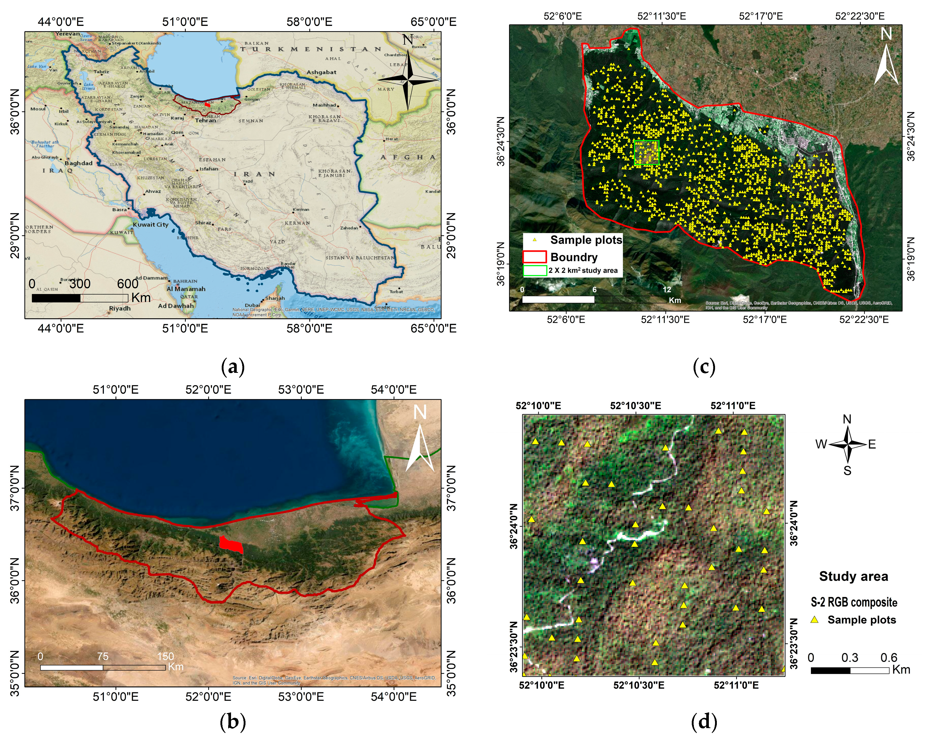
2.1. Study Area
2.2. Ground Controls (GCs), Data, and Sample Plots
2.3. Remote Sensing Data
3. Methodology
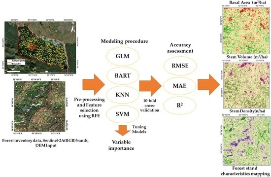
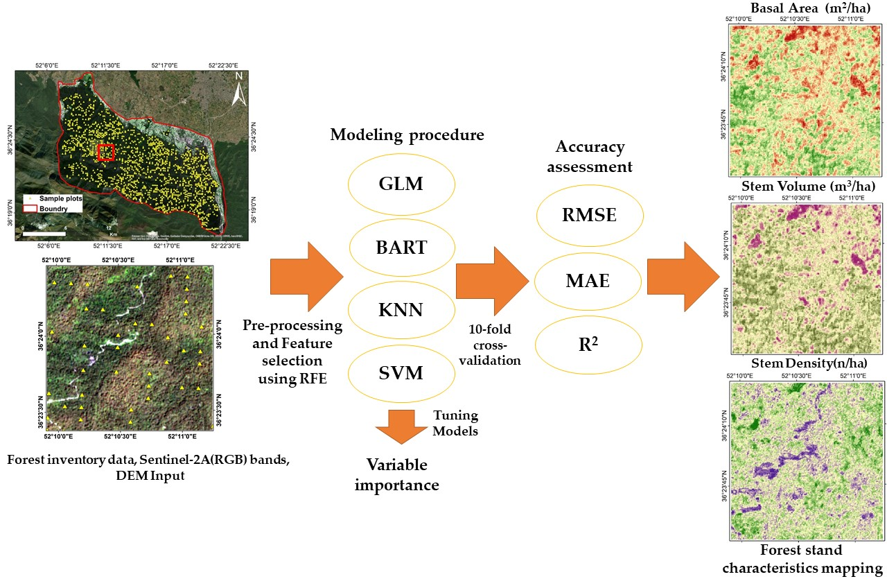
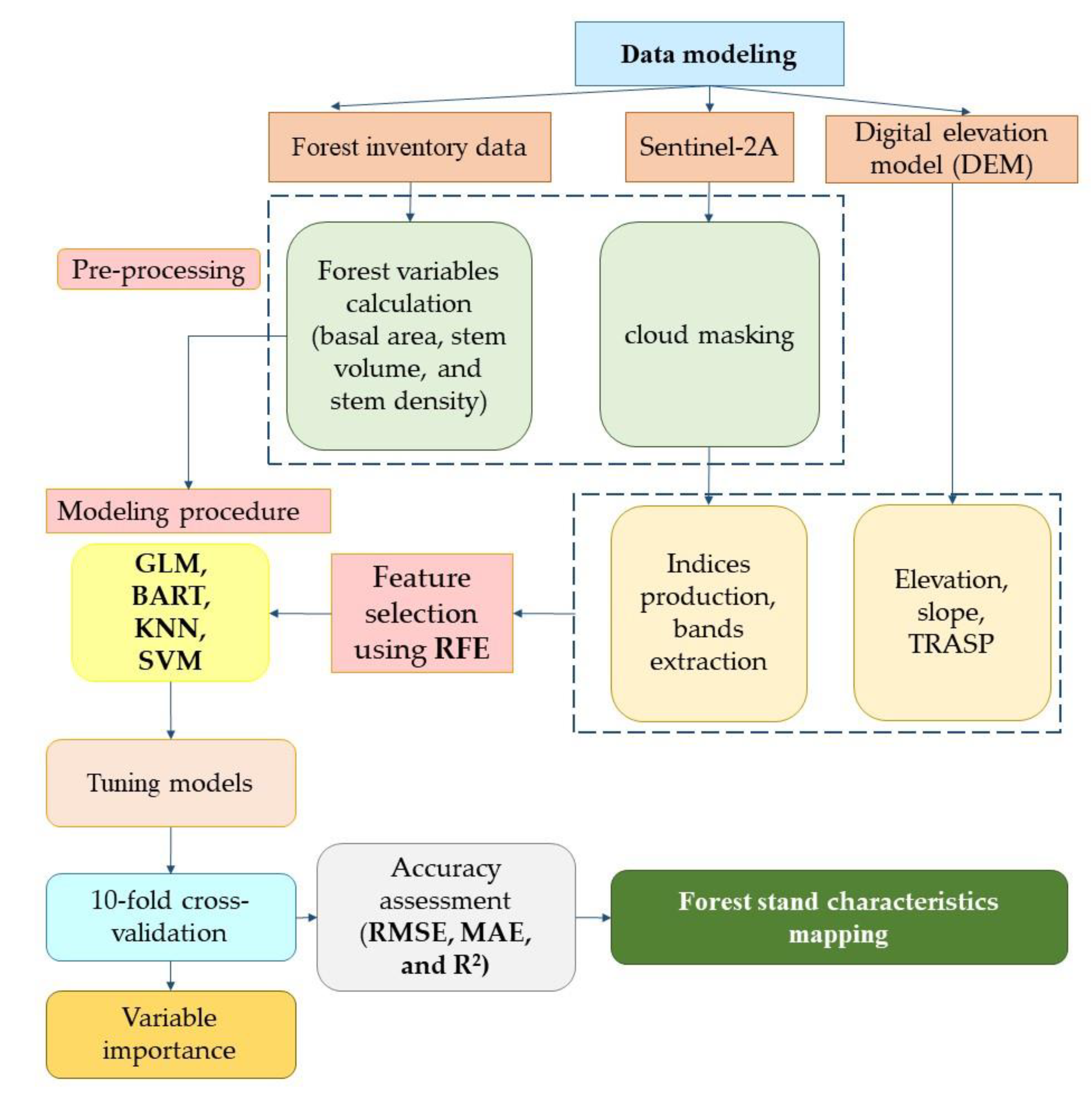
3.1. Overview
3.2. Pre-Processing
3.3. Feature Computation, Extraction, and Selection
3.3.1. Topographic Feature Computation
3.3.2. Indices and Band Extraction

| Predictors | Description | Ref |
|---|---|---|
| B1 | Coastal aerosol | - |
| B2 | Blue | - |
| B3 | Green | - |
| B4 | Red | - |
| B5 | Red-edge-1 (RE1) | - |
| B6 | Red-edge-2 (RE2) | - |
| B7 | Red-edge-3 (RE3) | - |
| B8 | Near infrared (NIR) | - |
| B8A | NIR plateau (NIRp) | - |
| B11 | Shortwave infrared (SWIR-1) | - |
| B12 | SWIR-2 | - |
| DVI | [13] | |
| NDVI | [13] | |
| MSAVI | [50] | |
| MSAVI2 | [47] | |
| GNDVI | [22] | |
| IPVI | [22] | |
| IRECI | [47] | |
| NDI45 | [47] | |
| PSSRA | [47] | |
| PVI | [47] | |
| RVI | [47] | |
| SAVI | [22] | |
| TNDVI | [47] | |
| WDVI | [47] | |
| Elevation | Digital elevation model | |
| Slope | ||
| TRASP | [51] | |
| Description: |
3.3.3. Feature Selection
3.4. Machine Learning Methods
3.4.1. Generalised Linear Model (GLM)
3.4.2. K–Nearest Neighbour (KNN)
3.4.3. Support Vector Machine (SVM)
3.4.4. Bayesian Additive Regression Trees (BART)
3.5. Model Evaluation
3.5.1. Root Mean Square Error (RMSE)
3.5.2. Mean Absolute Error (MAE)
3.5.3. R-Squared (R2)
4. Results
| Stand Characteristics | ||||
|---|---|---|---|---|
| Predictors | Original Resolution (m) | Basal area | Volume | Density |
| B1 | 60 | - | - | - |
| B2 | 10 | - | - | + |
| B3 | 10 | - | + | + |
| B4 | 10 | - | - | + |
| B5 | 20 | + | + | - |
| B6 | 20 | + | + | - |
| B7 | 20 | - | + | + |
| B8 | 10 | - | + | - |
| B8A | 20 | + | - | - |
| B11 | 20 | + | + | + |
| B12 | 20 | + | + | + |
| DVI | 10 | - | - | - |
| NDVI | 10 | - | + | - |
| MSAVI | 10 | - | - | + |
| MSAVI2 | 10 | - | - | - |
| GNDVI | 10 | - | - | + |
| IPVI | 10 | - | - | - |
| IRECI | 10 | + | + | + |
| NDI45 | 10 | + | - | + |
| PSSRA | 10 | + | + | + |
| PVI | 10 | - | - | - |
| RVI | 10 | - | + | + |
| SAVI | 10 | - | - | - |
| TNDVI | 10 | - | + | - |
| WDVI | 10 | - | - | + |
| Elevation | 12.5 | + | + | - |
| Slope | 12.5 | + | + | - |
| TRASP | 12.5 | + | + | - |
5. Discussion
6. Conclusions
Author Contributions
Funding
Acknowledgments
Conflicts of Interest
References
- Wietecha, M.; Jełowicki, Ł.; Mitelsztedt, K.; Miścicki, S.; Stereńczak, K. The capability of species-related forest stand characteristics determination with the use of hyperspectral data. Remote Sens. Environ. 2019, 231, 111232. [Google Scholar] [CrossRef]
- Nabuurs, G.J.; Masera, O.; Andrasko, K.; Benitez-Ponce, P.; Boer, R.; Dutschke, M.; Elsiddig, E.; Ford-Robertson, J.; Frumhoff, P.; Karjalainen, T.; et al. Forestry. Climate Change 2007: Mitigation. Contribution of Working Group III to the Fourth Assessment Report of the Intergovernmental Panel on Climate Change; Cambridge University Press: New York, NY, USA, 2007. [Google Scholar]
- Soares, P.; Tomé, M.; Skovsgaard, J.P.; Vanclay, J.K. Evaluating a growth model for forest management using continuous forest inventory data. For. Ecol. Manag. 1995, 71, 251–265. [Google Scholar] [CrossRef]
- Kitayama, K.; Fujiki, S.; Aoyagi, R.; Imai, N.; Sugau, J.; Titin, J.; Nilus, R.; Lagan, P.; Sawada, Y.; Ong, R.; et al. Biodiversity observation for land and ecosystem health (BOLEH): A robust method to evaluate the management impacts on the bundle of carbon and biodiversity ecosystem services in tropical production forests. Sustainability 2018, 10, 4224. [Google Scholar] [CrossRef] [Green Version]
- Roy, P.S.; Behera, M.D.; Srivastav, S.K. Satellite remote sensing: Sensors, applications and techniques. Proc. Natl. Acad. Sci. India Sect. A Phys. Sci. 2017, 87, 465–472. [Google Scholar] [CrossRef] [Green Version]
- Zahriban Heasari, M.; Fallah, A.; Shataee, S.; Kalbi, S.; Persson, H. Estimating the forest stand volume and basal area using pleiades spectral and auxiliary data. ISPRS Int. Arch. Photogramm. Remote Sens. Spat. Inf. Sci. 2019, 42, 1131–1136. [Google Scholar] [CrossRef] [Green Version]
- Kumar, M.; Singh, M.P.; Singh, H.; Dhakate, P.M.; Ravindranath, N.H. Forest working plan for the sustainable management of forest and biodiversity in India. J. Sustain. For. 2020, 39, 1–22. [Google Scholar] [CrossRef]
- Maponya, M.G.; Van Niekerk, A.; Mashimbye, Z.E. Pre-Harvest classification of crop types using a Sentinel-2 time-series and machine learning. Comput. Electron. Agric. 2020, 169, 105164. [Google Scholar] [CrossRef]
- Ji, C.; Li, X.; Wei, H.; Li, S. Comparison of different multispectral sensors for photosynthetic and non-photosynthetic vegetation-fraction retrieval. Remote Sens. 2020, 12, 115. [Google Scholar] [CrossRef] [Green Version]
- Grabska, E.; Hostert, P.; Pflugmacher, D.; Ostapowicz, K. Forest stand species mapping using the sentinel-2 time series. Remote Sens. 2019, 11, 1197. [Google Scholar] [CrossRef] [Green Version]
- Luther, J.E.; Fournier, R.A.; Van Lier, O.R.; Bujold, M. Extending ALS-based mapping of forest attributes with medium resolution satellite and environmental data. Remote Sens. 2019, 11, 1092. [Google Scholar] [CrossRef] [Green Version]
- Ottosen, T.-B.; Petch, G.; Hanson, M.; Skjøth, C.A. Tree cover mapping based on Sentinel-2 images demonstrate high thematic accuracy in Europe. Int. J. Appl. Earth Obs. Geoinf. 2020, 84, 101947. [Google Scholar]
- Sothe, C.; De Almeida, C.M.; Liesenberg, V.; Schimalski, M.B. Evaluating Sentinel-2 and Landsat-8 data to map sucessional forest stages in a subtropical forest in Southern Brazil. Remote Sens. 2017, 9, 838. [Google Scholar]
- Puletti, N.; Chianucci, F.; Castaldi, C. Use of Sentinel-2 for forest classification in Mediterranean environments. Ann. Silvic. Res 2018, 42, 32–38. [Google Scholar]
- Szostak, M.; Hawryło, P.; Piela, D. Using of Sentinel-2 images for automation of the forest succession detection Using of Sentinel-2 images for automation of the forest succession detection. Eur. J. Remote Sens. 2018, 51, 142–149. [Google Scholar]
- Frampton, W.J.; Dash, J.; Watmough, G.; Milton, E.J. Evaluating the capabilities of Sentinel-2 for quantitative estimation of biophysical variables in vegetation. ISPRS J. Photogramm. Remote Sens. 2013, 82, 83–92. [Google Scholar]
- Majasalmi, T.; Rautiainen, M. The potential of Sentinel-2 data for estimating biophysical variables in a boreal forest: A simulation study. Remote Sens. Lett. 2016, 7, 427–436. [Google Scholar]
- Addabbo, P.; Focareta, M.; Marcuccio, S.; Votto, C.; Ullo, S.L. Contribution of Sentinel-2 data for applications in vegetation monitoring. Acta IMEKO 2016, 5, 44–54. [Google Scholar]
- Lu, D.; Mausel, P.; Brondízio, E.; Moran, E. Relationships between forest stand parameters and Landsat TM spectral responses in the Brazilian Amazon Basin. For. Ecol. Manag. 2004, 198, 149–167. [Google Scholar]
- Astola, H.; Häme, T.; Sirro, L.; Molinier, M.; Kilpi, J. Comparison of Sentinel-2 and Landsat 8 imagery for forest variable prediction in boreal region. Remote Sens. Environ. 2019, 223, 257–273. [Google Scholar]
- Immitzer, M.; Vuolo, F.; Atzberger, C. First experience with Sentinel-2 data for crop and tree species classifications in central Europe. Remote Sens. 2016, 8, 166. [Google Scholar]
- Bolyn, C.; Michez, A.; Gaucher, P.; Lejeune, P.; Bonnet, S. Forest mapping and species composition using supervised per pixel classification of sentinel-2 imagery. Biotechnol. Agron. Soc. Environ. 2018, 22, 172–187. [Google Scholar]
- Hościło, A.; Lewandowska, A. Mapping forest type and tree species on a regional scale using multi-temporal Sentinel-2 data. Remote Sens. 2019, 11, 929. [Google Scholar]
- Zhao, Q.; Yu, S.; Zhao, F.; Tian, L.; Zhao, Z. Comparison of machine learning algorithms for forest parameter estimations and application for forest quality assessments. For. Ecol. Manag. 2019, 434, 224–234. [Google Scholar] [CrossRef]
- Fragou, S.; Kalogeropoulos, K.; Stathopoulos, N.; Louka, P.; Srivastava, P.; Karpouzas, S.; Kalivas, D.P.; Petropoulos, G.P. Quantifying land cover changes in a mediterranean environment using Landsat TM and Support Vector Machines. Forests 2020, 11, 750. [Google Scholar] [CrossRef]
- Galgamuwa, G.A.P.; Wang, J.; Barden, C.J. Expansion of eastern redcedar (Juniperus virginiana L.) into the deciduous woodlands within the forest-prairie ecotone of Kansas. Forests 2020, 11, 154. [Google Scholar]
- Noorian, N.; Shataee-Jouibary, S.; Mohammadi, J. Assessment of different remote sensing data for forest structural attributes estimation in the Hyrcanian forests. For. Syst. 2016, 25, 1–15. [Google Scholar] [CrossRef] [Green Version]
- Huang, Y.; Chen, Z.X.; Yu, T.; Huang, X.; Gu, X. Agricultural remote sensing big data: Management and applications. J. Integr. Agric. 2018, 17, 1915–1931. [Google Scholar]
- Sedona, R.; Cavallaro, G.; Jitsev, J.; Strube, A.; Riedel, M.; Benediktsson, J.A. Remote sensing big data classification with high performance distributed deep learning. Remote Sens. 2019, 11, 3056. [Google Scholar] [CrossRef] [Green Version]
- Copernicus Space Component Mission Management Team. Sentinel High Level Operations Plan (HLOP): COPES1OP-EOPG-PL-15-0020. Available online: https://earth.esa.int/documents/247904/685154/Sentinel_High_Level_Operations_Plan (accessed on 17 August 2020).
- Sudmanns, M.; Tiede, D.; Lang, S.; Bergstedt, H.; Trost, G.; Augustin, H.; Baraldi, A.; Blaschke, T. Big Earth data: Disruptive changes in Earth observation data management and analysis? Int. J. Digit. Earth 2020, 13, 832–850. [Google Scholar] [CrossRef]
- Lu, D.; Weng, Q. A survey of image classification methods and techniques for improving classification performance. Int. J. Remote Sens. 2007, 28, 823–870. [Google Scholar] [CrossRef]
- Andersen, R. Nonparametric methods for modeling nonlinearity in regression analysis. Annu. Rev. Sociol. 2009, 35, 67–85. [Google Scholar] [CrossRef]
- Noi, P.T.; Kappas, M. Comparison of random forest, k-nearest neighbor, and support vector machine classifiers for land cover classification using sentinel-2 imagery. Sensors 2018, 18, 18. [Google Scholar]
- Gajardo, J.; García, M.; Riaño, D. Applications of airborne laser scanning in forest fuel assessment and fire prevention. In Forestry Applications of Airborne Laser Scanning Concepts and Case Studies; Maltamo, M., Naesset, E., Vauhkonen, J., Eds.; Springer: Dodrecht, The Netherlands, 2014; ISBN 9789401786621. [Google Scholar]
- Safari, A.; Sohrabi, H.; Powell, S.; Shataee, S. A comparative assessment of multi-temporal Landsat 8 and machine learning algorithms for estimating aboveground carbon stock in coppice oak forests. Int. J. Remote Sens. 2017, 38, 6407–6432. [Google Scholar] [CrossRef]
- McCord, S.E.; Buenemann, M.; Karl, J.W.; Browning, D.M.; Hadley, B.C. Integrating remotely sensed imagery and existing multiscale field data to derive rangeland indicators: Application of Bayesian Additive Regression Trees. Rangel. Ecol. Manag. 2017, 70, 644–655. [Google Scholar] [CrossRef]
- Ali, I.; Greifeneder, F.; Stamenkovic, J.; Neumann, M.; Notarnicola, C. Review of machine learning approaches for biomass and soil moisture retrievals from remote sensing data. Remote Sens. 2015, 7, 16398–16421. [Google Scholar] [CrossRef] [Green Version]
- Bayat, M.; Ghorbanpour, M.; Zare, R.; Jaafari, A.; Thai Pham, B. Application of artificial neural networks for predicting tree survival and mortality in the Hyrcanian forest of Iran. Comput. Electron. Agric. 2019, 164, 104929. [Google Scholar] [CrossRef]
- Chipman, H.A.; George, E.I.; McCulloch, R.E. BART: Bayesian additive regression trees. Ann. Appl. Stat. 2010, 4, 266–298. [Google Scholar] [CrossRef]
- Izadi, S.; Sohrabi, H.; Khaledi, M.J. Estimation of coppice forest characteristics using spatial and non-spatial models and Landsat data. J. Spat. Sci. 2020, 1–14. [Google Scholar] [CrossRef]
- Clark, A.I.; Souter, R.A. Stem Cubic-Foot Volume Tables for Tree Species in the South; US Department of Agriculture, Forest Service, Southeastern Forest Experiment Station: Asheville, NC, USA, 1994; p. 252.
- Al-Najjar, H.A.H.; Kalantar, B.; Pradhan, B.; Saeidi, V.; Halin, A.A.; Ueda, N.; Mansor, S. Land cover classification from fused DSM and UAV images using convolutional neural networks. Remote Sens. 2019, 11, 1461. [Google Scholar] [CrossRef] [Green Version]
- Shanableh, A.; Al-Ruzouq, R.; Gibril, M.B.A.; Flesia, C.; Al-Mansoori, S. Spatiotemporal Mapping and Monitoring of Whiting in the Semi-Enclosed Gulf Using Moderate Resolution Imaging Spectroradiometer (MODIS) Time Series Images and a Generic Ensemble Tree-Based Model. Remote Sens. 2019, 11, 1193. [Google Scholar] [CrossRef] [Green Version]
- Ball, L.; Tzanopoulos, J. Interplay between topography, fog and vegetation in the central South Arabian mountains revealed using a novel Landsat fog detection technique. Remote Sens. Ecol. Conserv. 2020, 1–16. [Google Scholar] [CrossRef] [Green Version]
- Ahmadi, K.; Jalil Alavi, S.; Zahedi Amiri, G.; Mohsen Hosseini, S.; Serra-Diaz, J.M.; Svenning, J.C. Patterns of density and structure of natural populations of Taxus baccata in the Hyrcanian forests of Iran. Nord. J. Bot. 2020, 38, 1–10. [Google Scholar] [CrossRef]
- Rozenstein, O.; Haymann, N.; Kaplan, G.; Tanny, J. Validation of the cotton crop coefficient estimation model based on Sentinel-2 imagery and eddy covariance measurements. Agric. Water Manag. 2019, 223, 105715. [Google Scholar] [CrossRef]
- Shataee, S.; Kalbi, S.; Fallah, A.; Pelz, D. Forest attribute imputation using machine-learning methods and ASTER data: Comparison of k-NN, SVR and random forest regression algorithms. Int. J. Remote Sens. 2012, 33, 6254–6280. [Google Scholar] [CrossRef]
- Adeyeri, O.E.; Akinsanola, A.A.; Ishola, K.A. Investigating surface urban heat island characteristics over Abuja, Nigeria: Relationship between land surface temperature and multiple vegetation indices. Remote Sens. Appl. Soc. Environ. 2017, 7, 57–68. [Google Scholar] [CrossRef]
- Qi, J.; Chehbouni, A.; Huete, A.R.; Kerr, Y.H.; Sorooshian, S. A modified soil adjusted vegetation index. Remote Sens. Environ. 1994, 48, 119–126. [Google Scholar] [CrossRef]
- Hammer, E.S.; Walsh, S.J. Canopy Structure in the Krummholz and Patch Forest Zones. In The Changing Alpine Treeline; Butler, D.R., Malanson, G.P., Wals, S.J., Fagre, D.B., Eds.; Elsevier: Amsterdam, The Netherlands, 2009; Volume 12, ISBN 9780444533647. [Google Scholar]
- Kuhn, M.; Johnson, K. Applied Predictive Modeling; Springer: New York, NY, USA, 2013; ISBN 9781461468493. [Google Scholar]
- Lebedev, A.V.; Westman, E.; Van Westen, G.J.P.; Kramberger, M.G.; Lundervold, A.; Aarsland, D.; Soininen, H.; Kłoszewska, I.; Mecocci, P.; Tsolaki, M.; et al. Random forest ensembles for detection and prediction of Alzheimer’s disease with a good between-cohort robustness. NeuroImage Clin. 2014, 6, 115–125. [Google Scholar] [CrossRef] [Green Version]
- Yan, K.; Zhang, D. Feature selection and analysis on correlated gas sensor data with recursive feature elimination. Sens. Actuators B Chem. 2015, 212, 353–363. [Google Scholar] [CrossRef]
- Kuhn, M. Building predictive models in R using the caret package. J. Stat. Softw. 2008, 28, 1–26. [Google Scholar] [CrossRef] [Green Version]
- Li, W.; Niu, Z.; Chen, H.; Li, D.; Wu, M.; Zhao, W. Remote estimation of canopy height and aboveground biomass of maize using high-resolution stereo images from a low-cost unmanned aerial vehicle system. Ecol. Indic. 2016, 67, 637–648. [Google Scholar] [CrossRef]
- Varvia, P.; Lähivaara, T.; Maltamo, M.; Packalen, P.; Seppänen, A. Gaussian process regression for forest attribute estimation from airborne laser scanning data. IEEE Trans. Geosci. Remote Sens. 2019, 57, 3361–3369. [Google Scholar]
- Li, X.; Wang, Y. Applying various algorithms for species distribution modelling. Integr. Zool. 2013, 8, 124–135. [Google Scholar] [PubMed]
- Youssef, A.M.; Pradhan, B.; Pourghasemi, H.R.; Abdullahi, S. Landslide susceptibility assessment at Wadi Jawrah Basin, Jizan region, Saudi Arabia using two bivariate models in GIS. Geosci. J. 2015, 19, 449–469. [Google Scholar]
- James, G.; Witten, D.; Hastie, T.; Tibshirani, R. An Introduction to Statistical Learning—With Applications in R; Springer: Berlin/Heidelberg, Germany, 2013; ISBN 9781461471370. [Google Scholar]
- Myers, R.H.; Montgomery, D.C.; Vining, G.G.; Robinson, T.J. Generalized Linear Models with Applications in Engineering and the Sciences, 2nd ed.; John Wiley & Sons, Inc.: Hoboken, NJ, USA, 2002; Volume 95, ISBN 9780470454633. [Google Scholar]
- Naghibi, S.A.; Pourghasemi, H.R. A Comparative Assessment Between Three Machine Learning Models and Their Performance Comparison by Bivariate and Multivariate Statistical Methods in Groundwater Potential Mapping Learning Models and Their Performance Comparison by Bivariate and Multivaria. Water Resour. Manag. 2015, 29, 5217–5236. [Google Scholar]
- McRoberts, R.E. Forest ecology and management estimating forest attribute parameters for small areas using nearest neighbors techniques. For. Ecol. Manag. 2012, 272, 3–12. [Google Scholar]
- Khan, M.; Ding, Q.; Perrizo, W. K-Nearest neighbor classification on spatial data streams using P-trees. In Lecture Notes in Computer Science, Proceedings of the Pacific-Asia Conference on Knowledge Discovery and Data Mining, Taipei, Taiwan, 6-8 May 2002; Springer: Berlin/Heidelberg, Germany, 2002; Volume 2336, pp. 517–528. [Google Scholar]
- Lang, M.; Arumäe, T.; Lükk, T.; Sims, A. Estimation of standing wood volume and species composition in managed nemoral multi-layer mixed forests by using nearest neighbour classifier, multispectral satellite images and airborne lidar data. For. Stud. 2014, 61, 47–68. [Google Scholar]
- Kalantar, B.; Pradhan, B.; Naghibi, S.A.; Motevalli, A.; Mansor, S. Assessment of the effects of training data selection on the landslide susceptibility mapping: A comparison between support vector machine (SVM), logistic regression (LR) and artificial neural networks (ANN). Geomat. Nat. Hazards Risk 2018, 9, 49–69. [Google Scholar]
- Tan, Y.V.; Roy, J. Bayesian additive regression trees and the general BART model. Stat. Med. 2019, 38, 5048–5069. [Google Scholar]
- Ghorbanzadeh, O.; Rostamzadeh, H.; Blaschke, T.; Gholaminia, K.; Aryal, J. A new GIS-based data mining technique using an adaptive neuro-fuzzy inference system (ANFIS) and k-fold cross-validation approach for land subsidence susceptibility mapping. Nat. Hazards 2018, 94, 497–517. [Google Scholar]
- Lindberg, E.; Hollaus, M. Comparison of methods for estimation of stem volume, stem number and basal area from airborne laser scanning data in a hemi-boreal forest. Remote Sens. 2012, 4, 1004–1023. [Google Scholar]
- Khosravi, K.; Sartaj, M.; Tsai, F.T.C.; Singh, V.P.; Kazakis, N.; Melesse, A.M.; Prakash, I.; Tien Bui, D.; Pham, B.T. A comparison study of DRASTIC methods with various objective methods for groundwater vulnerability assessment. Sci. Total Environ. 2018, 642, 1032–1049. [Google Scholar] [CrossRef] [PubMed]
- Opitz, D.; Blundell, S. An AFE approach for combining LIDAR and color imagery background: Feature analyst and LIDAR analyst. In Proceedings of the ASPRS 2008 Annual Conference, Portland, OR, USA, 28 April–2 May 2008. [Google Scholar]
- Zhao, P.; Gao, L.; Gao, T. Extracting forest parameters based on stand automatic segmentation algorithm. Sci. Rep. 2020, 10, 1–13. [Google Scholar] [CrossRef] [PubMed] [Green Version]
- Piñeiro, G.; Perelman, S.; Guerschman, J.P.; Paruelo, J.M. How to evaluate models: Observed vs. predicted or predicted vs. observed? Ecol. Modell. 2008, 216, 316–322. [Google Scholar] [CrossRef]
- Mauya, E.W.; Koskinen, J.; Tegel, K.; Hämäläinen, J.; Kauranne, T.; Käyhkö, N. Modelling and predicting the growing stock volume in small-scale plantation forests of tanzania using multi-sensor image synergy. Forests 2019, 10, 279. [Google Scholar] [CrossRef] [Green Version]
- Vafaei, S.; Soosani, J.; Adeli, K.; Fadaei, H.; Naghavi, H.; Pham, T.D.; Bui, D.T. Improving accuracy estimation of forest aboveground biomass based on incorporation of ALOS-2 PALSAR-2 and Sentinel-2A imagery and machine learning: A case study of the Hyrcanian forest area (Iran). Remote Sens. 2018, 10, 172. [Google Scholar] [CrossRef] [Green Version]
- Valbuena, R.; Hernando, A.; Manzanera, J.A.; Görgens, E.B.; Almeida, D.R.A.; Silva, C.A.; García-Abril, A. Evaluating observed versus predicted forest biomass: R-squared, index of agreement or maximal information coefficient? Eur. J. Remote Sens. 2019, 52, 1–14. [Google Scholar] [CrossRef] [Green Version]
- Fatehi, P.; Damm, A.; Leiterer, R.; Bavaghar, M.P.; Schaepman, M.E.; Kneubühler, M. Tree density and forest productivity in a heterogeneous alpine environment: Insights from airborne laser scanning and imaging spectroscopy. Forests 2017, 8, 212. [Google Scholar] [CrossRef] [Green Version]
- Arévalo-Sandi, A.; Bobrowiec, P.E.D.; Chuma, V.J.U.R.; Norris, D. Diversity of terrestrial mammal seed dispersers along a lowland Amazon forest regrowth gradient. PLoS ONE 2018, 13, e0193752. [Google Scholar] [CrossRef] [Green Version]


| Application | Data | Models | Reference |
|---|---|---|---|
| Estimation of bio-physical variables of vegetation | Sentinel-2 | Vegetation indices assessment | [16] |
| Physically-based reflectance model (PARAS) | [17] | ||
| Classification of agricultural and tree species | Sentinel-2 | Random Forest (RF) | [21] |
| Land use/cover and forest detection | Sentinel-2 | Object-based image analysis (OBIA) | [15] |
| Tree cover mapping (forest/non forest and broadleaved/coniferous forest) | Sentinel-2 | k-means | [12] |
| Forest type mapping | Sentinel-2 | RF | [14] |
| Classification of forest tree species | Sentinel-2 | RF | [10] [22] [7] [13] |
| Sentinel-2 and DEM | [23] | ||
| Vegetation monitoring | Sentinel-1 and 2 and Landsat 8 | Vegetation indices assessment | [18] |
| Estimation of forest stand parameters | Sentinel-2 and Landsat 8 | Multi-layer perceptron neural network and regression tree | [20] |
| Mapping of forest attributes | Sentinel-2 data, PALSAR, airborne laser scanner, DEM | Multiple linear regression and RF | [11] |
| Estimating the forest stand volume and basal area | Pleiades data and climate data | RF | [6] |
| Forest parameters estimations (e.g., stand age, aboveground biomass, leaf area index, tree height, crown diameter) | Quickbird | Classification and regression tree (CART), SVM, ANN, and RF | [24] |
| Classification/change detection of tree species | Landsat TM time series | SVM | [25] |
| Hyperspectral data from HySpex VNIR-1800 and SWIR-384 | [1] | ||
| Tree species compositional changes | Landsat TM time series | K-means and iterative self-organizing data analysis technique (ISODATA), maximum likelihood, and SVM | [26] |
| Relationships between forest stand parameters and vegetation indices (e.g., volume, basal area, biomass, vegetation density, tree height) | Landsat TM | Vegetation indices assessment | [19] |
| Estimation of the forest structural attributes (e.g., stand volume, basal area, and tree stem density) | Landsat-5 TM, ASTER, and Quickbird | CART | [27] |
| Stand Variables | Descriptive Statistics | |||
|---|---|---|---|---|
| Minimum | Maximum | Mean | SD | |
| Basal Area (m2/ha) | 63.35 | 125.29 | 95.42 | 11.29 |
| Volume (m3/ha) | 138.4 | 371.10 | 256.07 | 41.67 |
| Density (n/ha) | 90 | 420.00 | 232.27 | 62.10 |
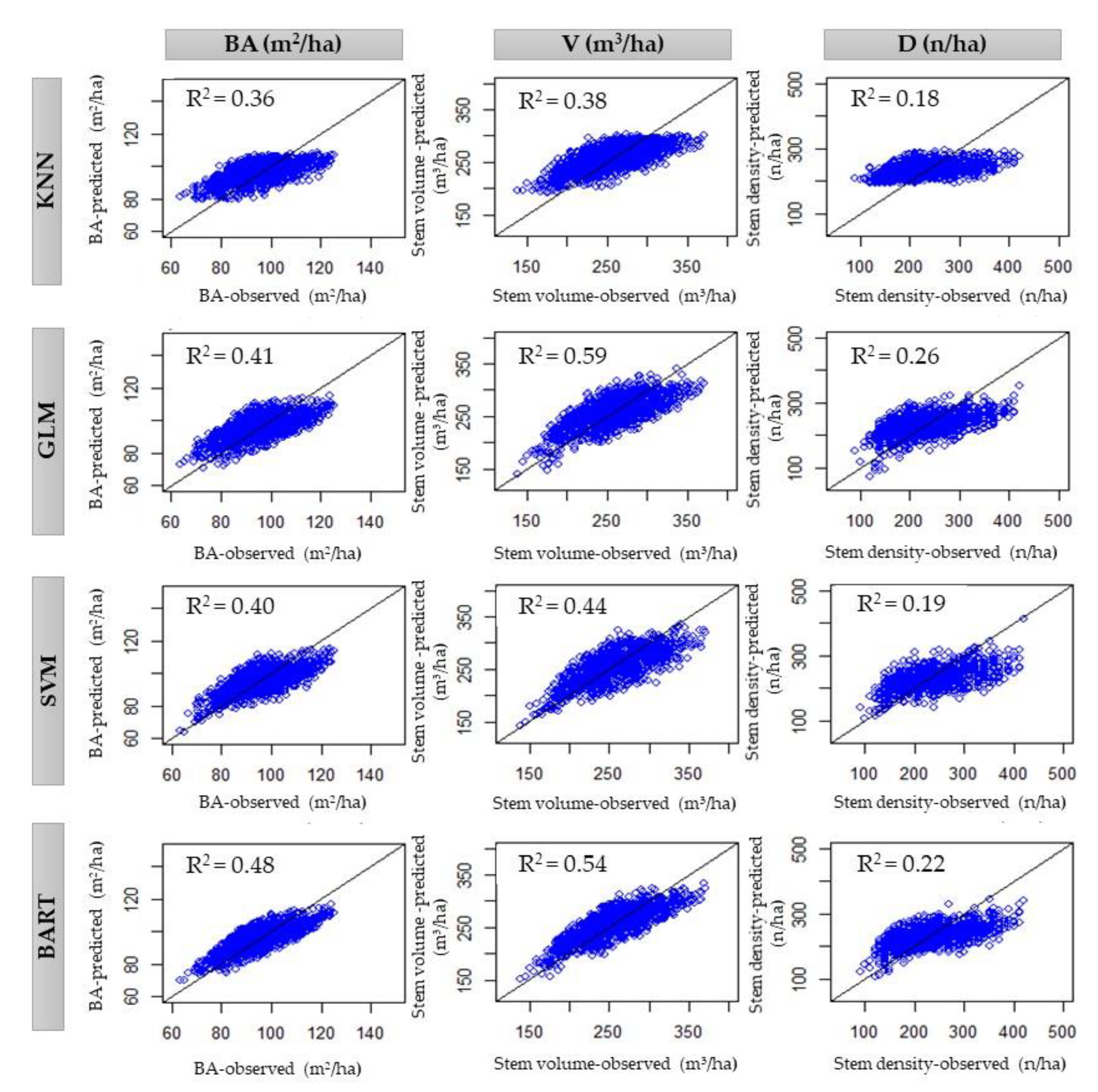
| Stand Variables | Models | ||||
|---|---|---|---|---|---|
| KNN | SVM | GLM | BART | ||
| Basal Area (m2/ha) | R2 | 0.36 | 0.40 | 0.41 | 0.48 |
| RMSE | 9.00 | 8.75 | 8.42 | 8.12 | |
| MAE | 7.55 | 7.31 | 7.18 | 6.88 | |
| %RMSE | 10.2 | 9.8 | 9.4 | 8.8 | |
| Stem Volume (m3/ha) | R2 | 0.38 | 0.44 | 0.59 | 0.54 |
| RMSE | 31.74 | 31.43 | 29.32 | 29.28 | |
| MAE | 26.50 | 26.14 | 24.78 | 24.53 | |
| %RMSE | 12.1 | 12.01 | 11.9 | 11.9 | |
| Stem Density (n/ha) | R2 | 0.18 | 0.19 | 0.26 | 0.22 |
| RMSE | 56.66 | 56.76 | 53.12 | 54.72 | |
| MAE | 46.88 | 45.91 | 43.87 | 45.08 | |
| %RMSE | 24.3 | 23.6 | 23.1 | 23.4 | |
© 2020 by the authors. Licensee MDPI, Basel, Switzerland. This article is an open access article distributed under the terms and conditions of the Creative Commons Attribution (CC BY) license (http://creativecommons.org/licenses/by/4.0/).
Share and Cite
Ahmadi, K.; Kalantar, B.; Saeidi, V.; Harandi, E.K.G.; Janizadeh, S.; Ueda, N. Comparison of Machine Learning Methods for Mapping the Stand Characteristics of Temperate Forests Using Multi-Spectral Sentinel-2 Data. Remote Sens. 2020, 12, 3019. https://doi.org/10.3390/rs12183019
Ahmadi K, Kalantar B, Saeidi V, Harandi EKG, Janizadeh S, Ueda N. Comparison of Machine Learning Methods for Mapping the Stand Characteristics of Temperate Forests Using Multi-Spectral Sentinel-2 Data. Remote Sensing. 2020; 12(18):3019. https://doi.org/10.3390/rs12183019
Chicago/Turabian StyleAhmadi, Kourosh, Bahareh Kalantar, Vahideh Saeidi, Elaheh K. G. Harandi, Saeid Janizadeh, and Naonori Ueda. 2020. "Comparison of Machine Learning Methods for Mapping the Stand Characteristics of Temperate Forests Using Multi-Spectral Sentinel-2 Data" Remote Sensing 12, no. 18: 3019. https://doi.org/10.3390/rs12183019