Classification of Australian Waterbodies across a Wide Range of Optical Water Types
by
 , , , and
Elizabeth J. Botha
1,* ,
,
Janet M. Anstee
1,
Stephen Sagar
2,
Eric Lehmann
3 and
Thais A. G. Medeiros
4
1
CSIRO Oceans & Atmosphere, Canberra, ACT 2601, Australia
2
Geoscience Australia, Symonston, ACT 2601, Australia
3
CSIRO Data61, Canberra, ACT 2601, Australia
4
National Institute for Space Research (INPE), Remote Sensing Division, Av. dos Astronautas 1758, São Jose dos Campos 12227-010, Brazil
*
Author to whom correspondence should be addressed.
Remote Sens. 2020, 12(18), 3018; https://doi.org/10.3390/rs12183018
Submission received: 25 August 2020
/
Revised: 11 September 2020
/
Accepted: 14 September 2020
/
Published: 16 September 2020
(This article belongs to the Special Issue Remote Sensing of Inland Waters and Their Catchments)
Abstract
:Baseline determination and operational continental scale monitoring of water quality are required for reporting on marine and inland water progress to Sustainable Development Goals (SDG). This study aims to improve our knowledge of the optical complexity of Australian waters. A workflow was developed to cluster the modelled spectral response of a range of in situ bio-optical observations collected in Australian coastal and continental waters into distinct optical water types (OWTs). Following clustering and merging, most of the modelled spectra and modelled specific inherent optical properties (SIOP) sets were clustered in 11 OWTs, ranging from clear blue coastal waters to very turbid inland lakes. The resulting OWTs were used to classify Sentinel-2 MSI surface reflectance observations extracted over relatively permanent water bodies in three drainage regions in Eastern Australia. The satellite data classification demonstrated clear limnological and seasonal differences in water types within and between the drainage divisions congruent with general limnological, topographical, and climatological factors. Locations of unclassified observations can be used to inform where in situ bio-optical data acquisition may be targeted to capture a more comprehensive characterization of all Australian waters. This can contribute to global initiatives like the SDGs and increases the diversity of natural water in global databases.
1. Introduction
Operational continental scale monitoring and baseline determination of water quality are fundamental for reporting on marine and inland water Sustainable Development Goals (SDG). Surface water is an important global resource and plays an essential role in biochemical cycling, maintenance of biodiversity, human wellbeing, and prosperity [1,2]. In the Australian context, existing water quality information is often limited, and inland water, in particular, is not well represented in global datasets or even nationally. Incompatibilities in the content and scale of state and territory environment reports confound attempts to integrate water resource data into a consistent national reporting framework [3,4,5]. In addition, existing monitoring practices do not encompass the breadth of temporal and spatial scales required for standardized baseline establishment (SDG indicator 14.1.1) or reporting on continental scale indicators (SDG indicator 6.3.2) germane to human health, environmental sustainability, and economic prosperity.
Earth observation (EO) methods have the potential to provide a consistent reporting mechanism, providing synoptic coverage of spatial and temporal variations in water quality [2,6,7,8]. Water quality parameters that can be derived from EO data include chlorophyll and phycocyanin concentrations [6,8], coloured dissolved organic matter (CDOM) [9], the concentration of total suspended solids (TSS) [10,11], and descriptors of the light environment of the water column, such as Secchi disk depth (SDz) [7], vertical attenuation (Kd), water clarity [12,13], and water colour [14,15,16], among others. However, their application at a continental scale is restricted by a lack of regional data for parameterization and validation of water quality information [4].
Quantitative use of EO data for the synoptic assessment of aquatic water quality has increased in recent times. Retrieval of water quality information from EO data can provide an improved understanding of the spatial and temporal variability within water bodies for the resource managers by filling temporal gaps between periodic in situ observations. Freely available, medium resolution EO data, such as from the Landsat suite of sensors and Sentinel-2 provide a useful platform in which to investigate temporal changes in water quality across wide geographic scales, e.g., [11,17,18,19,20,21].
Methods implemented to retrieve water quality parameters are strongly determined by the scale under consideration (local, regional, or global). At the local scale, a locally tuned empirical algorithm can be successfully implemented to retrieve water quality data. Due to spatial variability in optically active water column constituents, empirical tuning using geographically limited, in situ data fail at the regional or global scale in areas with unique optical properties [22] or where the optical complexity of extreme events such as floods, blackwater events, or algal blooms are not captured in the empirical model [4]. For example, the SeaWiFS global chlorophyll algorithm (OC4) failed to accurately retrieve chlorophyll from satellite data in Antarctic waters [23] and sediment plumes off the Santa Barbara Channel [24].
The application of physics-based (analytical) methods to retrieve environmental variables from EO data offers a solution across a range of scales in optically complex aquatic regions. This approach is strongly driven by an understanding of the relationship between inherent optical properties (IOPs) and the water-leaving radiative signal, which is ultimately detected by the satellite borne sensor. Several quasi-analytical algorithms have been tested and specifically tuned to local water bodies, e.g., Tokyo Bay [25], Venice Lagoon [26], and Lake Constance [27]. Physics-based algorithms have also been implemented on a more regional basis in the English Channel and French Guiana [28], coastal Australia [29,30], the Adriatic Sea [31], and Florida and the Arabian Sea [32].
Optical water types (OWT) is one method implemented to facilitate the retrieval of water column constituent data. OWTs are defined as different water masses that are represented by a collection of similar optical characteristics of the water components, resulting in similar reflectances [33]. Classifications based on OWTs can provide information about the concentration of optically significant constituents in each class, offering the possibility to observe the trends and status of important biogeochemical and biological variables. OWTs can be implemented to empirically retrieve water column constituents, e.g., [31,34,35], train neural networks, e.g., [35,36] or parameterize bio optical models, as suggested by [34,37]. This knowledge can then be implemented into monitoring strategies that support the assessment metrics of the UN SDGs related to aquatic ecosystems, such as water quality retrieval, algal bloom detection, estimation of primary production, refining the distributions of biogeographic provinces, and developing indices of marine biodiversity.
Various methodologies were developed in aquatic remote sensing studies to classify OWTs. Most often, some form of cluster analysis is implemented in the process. Cluster analysis groups water into sets based upon differences in the magnitude and shape of reflectance using different degrees of implicit or explicit knowledge [1]. A selection of recent studies, classifying reflectance data of water into generalized OWTs on scales ranging from local to global is presented in Table 1.
Coastal and inland waters are generally considered optically complex ‘Case 2′ waters [6]. Therefore, the observed reflectance spectra from different Case 2 waters share common features, as their optics are a function of a high variability in the concentrations of different optically active constituents [38,39]. Due to the range of bio-optical properties in these zones, classifying these waters is a challenge [33]. In addition, atmospheric correction algorithm failures [40,41] and the high spatio-temporal variability in hydrodynamics and biological processes [38] makes the classification of these waters more arduous. Due to this complexity, much effort has been focused on classification of coastal and inland waters.

Table 1.
Selected literature on optical water type classification.
| Spectral Data | Classification | Dataset | Reference |
|---|---|---|---|
| SeaWiFS data | ED a Eigenvector | Northwest Atlantic | [42] |
| Normalized SeaWiFS data | ISODATA b | Global | [43] |
| In situ Rrs c | hierarchical | English Channel | [37] |
| In situ Rrs | FCM d | Global | [44] |
| In situ Rrs | FCM d | Chinese lakes | [45] |
| In situ Rrs | FCM d | Global lakes | [46] |
| In situ Rrs | thresholding | Yellow Sea | [47] |
| Normalized In situ Rrs | hierarchical | Eastern English Channel North Sea French Guiana | [33] |
| Normalized In situ Rrs | k-means | Global | [1] |
| Simulated rrs e | WFCM f | Estonia Finland | [48] |
a ED: Euclidian Distance, b ISODATA: Iterative Self-Organizing Data Analysis Technique, c Rrs: Remote sensing reflectance, d FCM: Fuzzy-c Means, e rrs: subsurface reflectance, f WFCM: Weighted Fuzzy-c Means.
Several studies have successfully implemented optical classification techniques to formulate OWTs at a global scale (e.g., [1,43,44,46]). However, apart from incorporating data from three Southern African reservoirs [35], most of these global studies used data collected predominantly in the Northern hemisphere. Most of the regional studies also report on areas in the Northern Hemisphere (Table 1). This study aims to improve our knowledge of the optical complexity of Australian coastal and continental waters. Although several regional datasets have been reported on, e.g., [49,50,51,52,53], this will be the first attempt at analysing the data at a continental scale in Australia. To this end, a database of observations, capturing a range of optical data based on seasonality and geography, was used to:
- Develop a method to define distinct OWTs.
- Create a set of synthetic generalized inherent optical properties (GIOPs), based on the key features of each unique OWT.
- Present a case study as an example of a potential application of implementing the GIOPs water quality monitoring at a drainage basin scale.
2. Materials and Methods
2.1. In Situ Data
2.1.1. Datasets
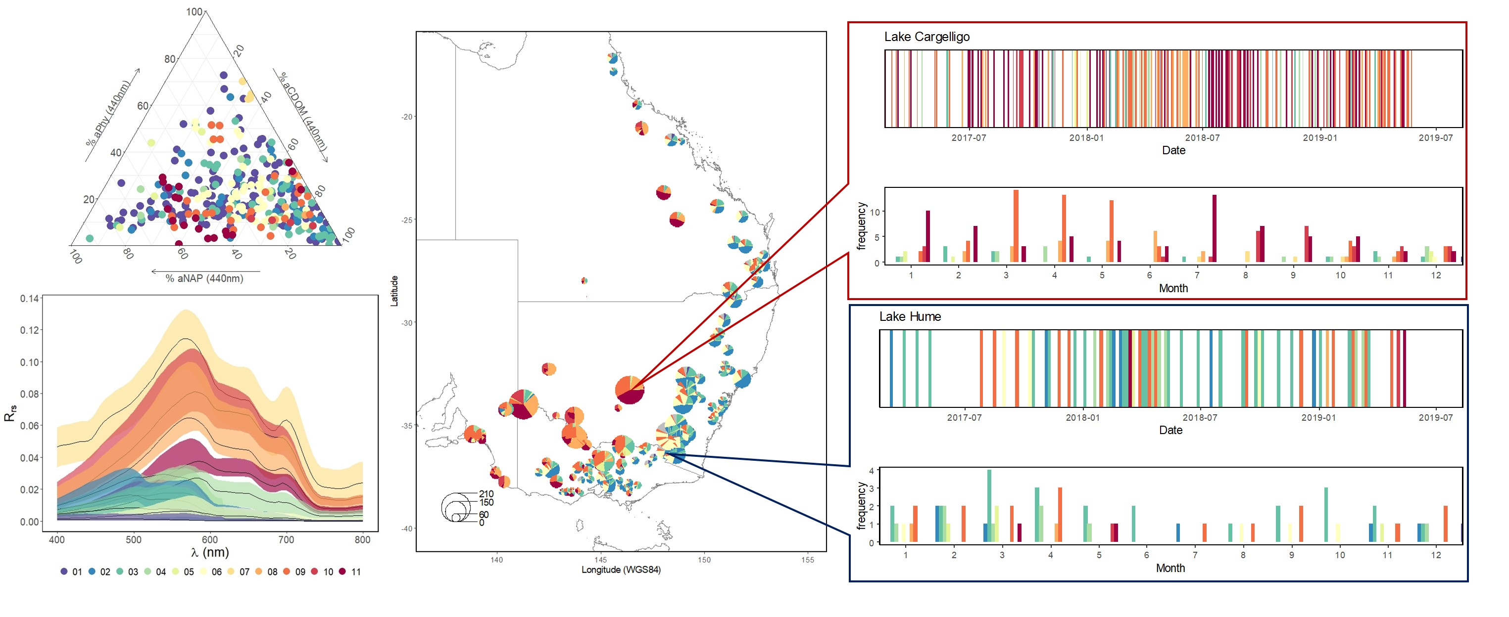
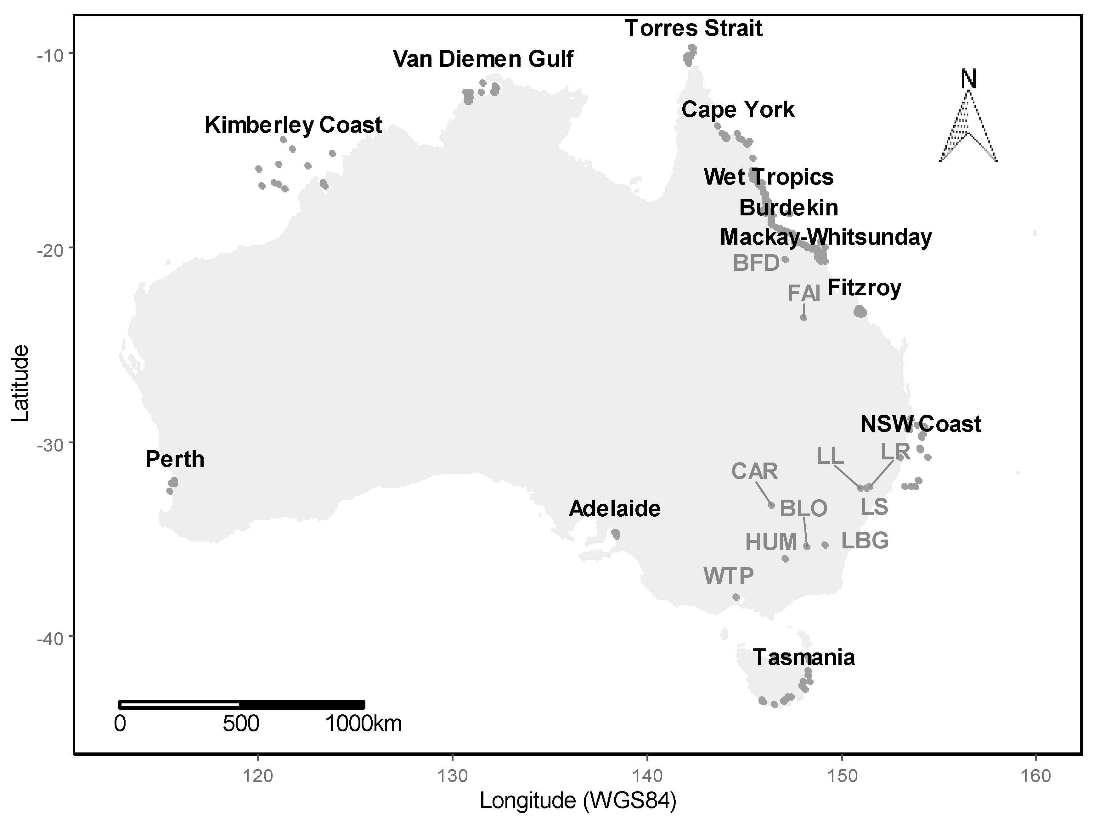
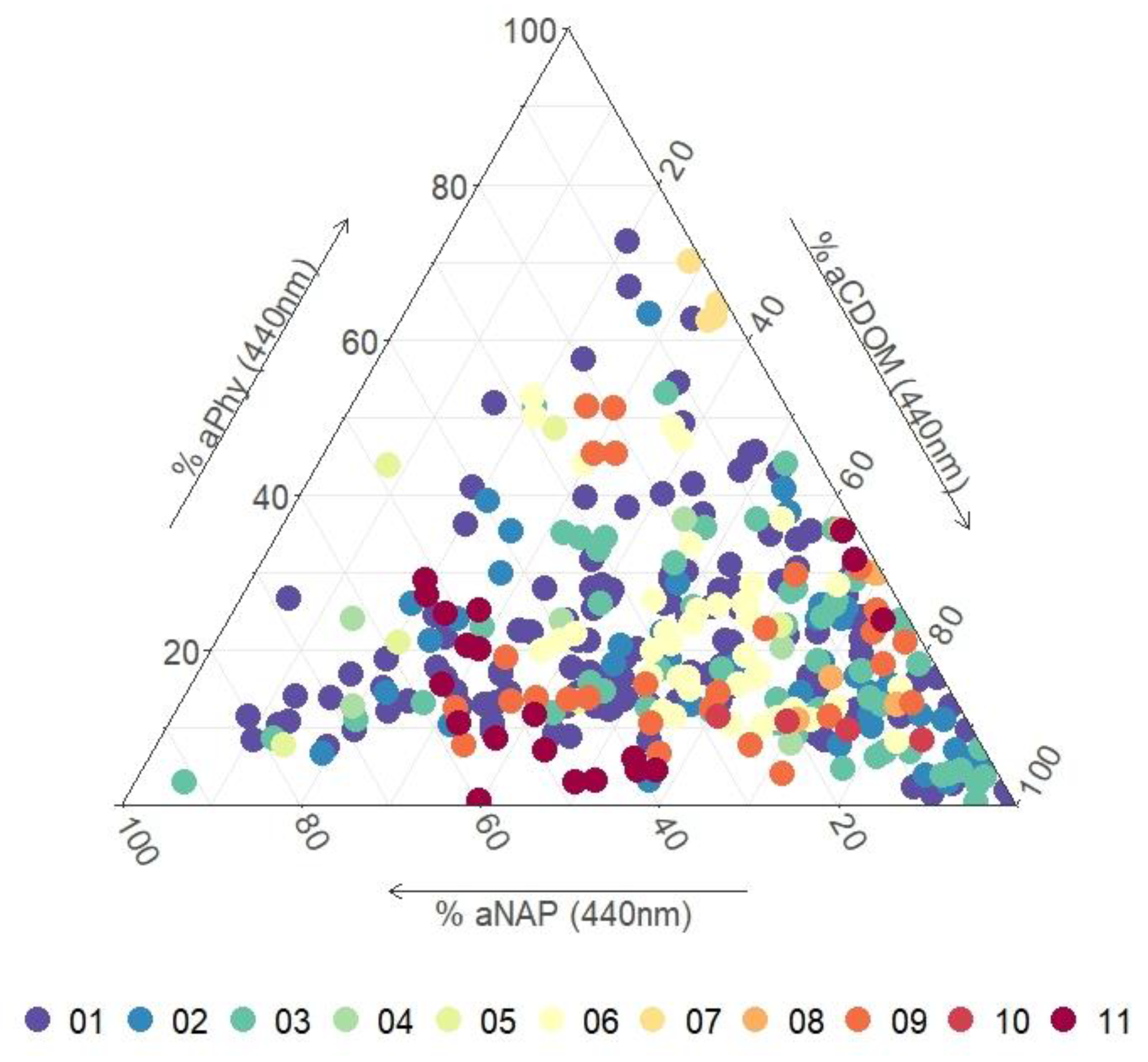
The observed reflectance spectra from coastal and inland waters share common features of Case 2 waters. Therefore, [44] proposed that coastal and inland waters may benefit from a common classification scheme, using aggregate data that provide continuity from fresh waters to marine environments. Thus, a database of 396 in situ measurements of specific inherent optical properties (SIOPs) and water quality concentrations of optically active water column, acquired in waterbodies around the Australian coast (Table S1) and along a latitudinal gradient in Eastern Australia (Table S2), was collated for analysis in this study. Figure 1 Shows the spatial distribution of sampling locations. Each record in the database represents quality assured observations collected at a single location with a complete description of optically active water column constituents and IOPs. A complete dataset comprises of in situ absorption and backscattering measurements as well as laboratory analysis of total suspended sediments, pigment analysis, and CDOM absorption. The protocols for sampling and sample analyses are comprehensively described in [54]. Figure 2a,b and Table 2 summarize the ranges of the IOPs used in this study while Figure 2c shows the absorption budget, demonstrating the range of the optically active water column constituents within the dataset.
2.1.2. Spectral Clustering
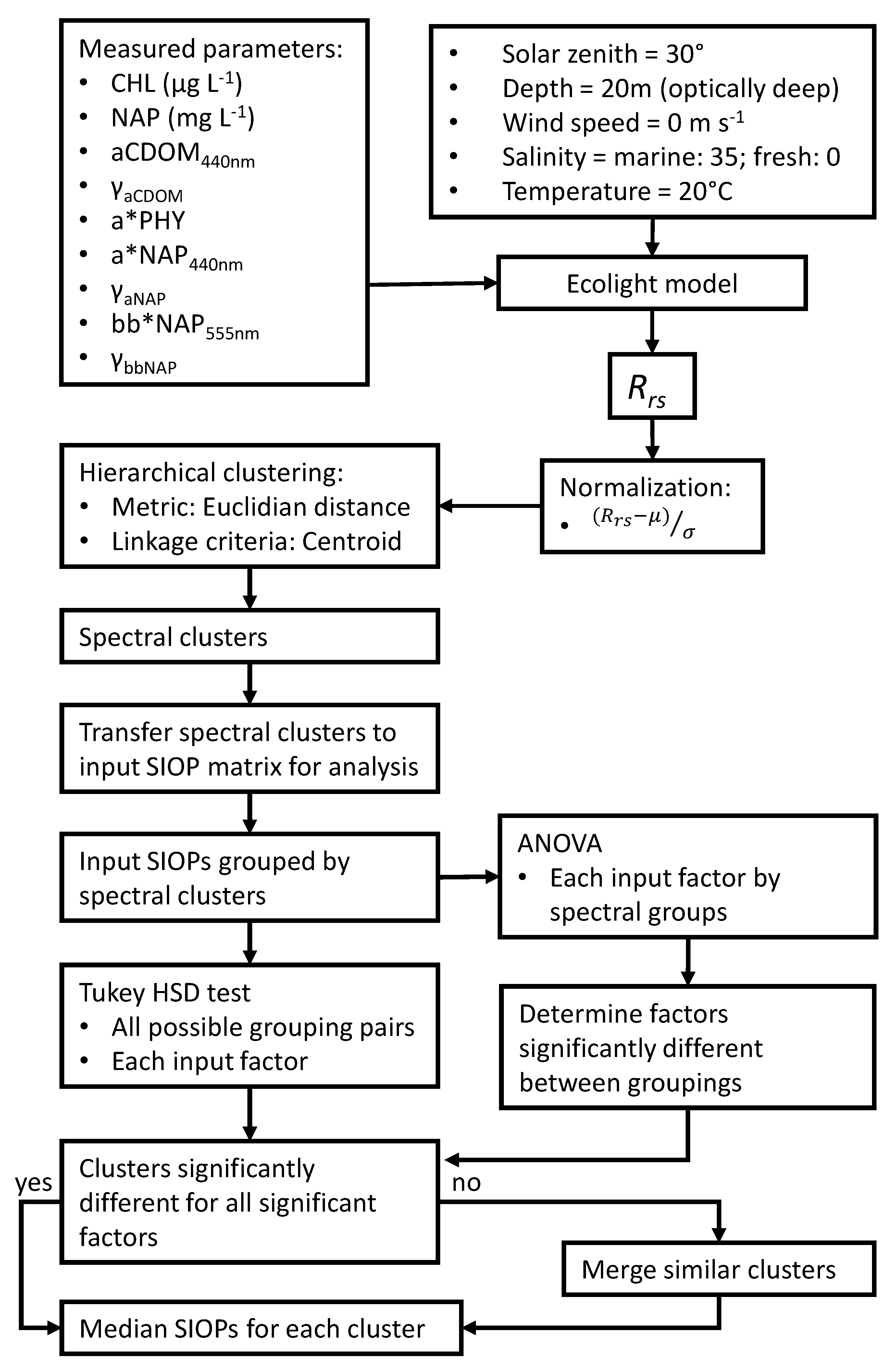
Most studies related to generalized OWTs are based on optical classification of in situ hyperspectral surface reflectance data (Rrs) (Table 1). However, surface reflectance, as an apparent optical property (AOP), is affected by water column optical properties and, to a lesser degree, on other environmental factors, such as sun and observations angles, atmospheric conditions, and sea-surface state [55,56]. There are also a diversity of radiometers and measurement protocols that can be implemented to measure AOPs, some of which are reviewed by [57]. This can potentially introduce spectral variations into an in situ dataset collated from numerous field campaigns. To ensure that the surface reflectance data used for this analysis represents the effects of only the water column, a modelling approach was implemented. This approach is like that of [48,58] where the authors classified coastal and open ocean waters, respectively, using simulated remote sensing reflectance (rrs). A summary of the data analysis approach used in this work is presented in Figure 3.
A four-component optical model (IOPs of the waterbody, water surface state, sky spectral radiance distribution, and the nature of the bottom boundary) was parameterized in Ecolight 5.0 (Sequoia Scientific, Inc., Bellevue, WA, USA) [59,60]. For all simulations, the sun zenith angle was set at 30° from nadir, wind speed was fixed at 0 m s−1, and the water column was assumed to be optically deep and homogeneous. Inelastic scattering was excluded. The IOP inputs, obtained from the bio-optical database, were thus the only factors contributing to spectral variability within the simulated spectra. The simulated surface reflectance spectra (Rrs) were produced at 5 nm spectral intervals between 350 nm and 800 nm.
Spectral clustering is usually based on one of two approaches: hierarchical or non-hierarchical. Hierarchical methods initially cluster the two most similar spectra together and then iterates, forming higher clusters until all the spectra are combined into a single cluster [37,61]. Non-hierarchical methods consider the overall distribution of spectral pairs and classifies them into a prescribed number of clusters. The most popular non-hierarchical clustering techniques is k-means and fuzzy-c means (e.g., [1,44,45,46]).
The simulated Rrs spectra in this study were subjected to hierarchical agglomerative clustering [61,62] where each spectrum was initially considered as a single-element cluster. At each step of the algorithm, a Euclidian distance (ED) metric was used to determine the two clusters that are the most similar [62,63]. These clusters were then combined into a new bigger cluster. This procedure was iterated until all points were members of just one single big cluster. A centroid linkage function was used to group pairs of objects into clusters based on their similarity [61]. This process was iterated until all the objects in the original dataset were linked together in a hierarchical tree.
To ensure the shape of the spectrum is adequately taken into consideration, the spectra were scaled prior to clustering. To preserve the shape of the spectra across the entire spectral range by not artificially giving a greater weight to a defined part of the Rrs spectra, normalization was based on the mean (μ) and standard deviation (σ) of the entire database [1,33]:
After spectral clustering, the SIOP data, used as input for each spectrum was analysed to determine whether the spectral clusters could be translated into unique SIOP groupings. A one-way ANOVA was applied to all the SIOP parameters in each of the spectral clusters to determine which parameters had the most significant effect on the spectral variability between classes. The parameters contributing most to spectral variability within the simulated spectral dataset were used to determine the SIOP separability between the different spectral clusters.
The SIOPs of clusters were compared with each other using a Tukey HSD test with a 95% family-wise confidence level [64]. Where the SIOPs closely resembled each other, clusters were merged into larger groupings. The resulting clusters were used to classify satellite-derived surface reflectance observations extracted over selected waterbodies in Eastern Australia.
2.2. Satellite Data
To capture enough variability in continental water quality to demonstrate the applicability of implementing the derived OWTs for temporal water quality monitoring at a drainage basin scale, a large temporal and spatial dataset is required [17,20,65]. Digital Earth Australia (DEA) provides analysis-ready (ARD) satellite data in the form of stacks of consistent, time-stamped surface reflectance observations. Using high-performance computing power provided by the National Computational Infrastructure (NCI) and commercial cloud computing platforms, DEA organizes and prepares the satellite data using Open Data Cube (ODC) technology [66]. Preparation includes geometric correction [67,68], atmospheric correction [69], and pixel quality flags [70,71,72].
For the purpose of this study, Sentinel-2 MSI satellite data were used. The Copernicus Sentinel-2 mission comprises a constellation of two polar-orbiting satellites placed in the same sun-synchronous orbit, phased at 180° to each other. Sentinel-2A was launched in June 2015 and Sentinel-2B in March 2017, creating a revisit time of 5 days. Sentinel-2 MSI has six spectral bands that are potentially useful for this study: Coastal aerosol (442 nm), blue (B, 490 nm), green (G, 560 nm), red (R, 665 nm), red-edge 1 (RE-1, 705 nm), and red-edge 2 (RE-2, 740 nm). However, the atmospheric correction protocol implemented on DEA is based on standard terrestrial aerosol climatology model parameters and processing. Consequently, it was found to have a large positive bias across the surface reflectance of all bands due to uncorrected aquatic specific influences such as sky and sun-glint. In addition, a shape distortion of the spectra between the coastal aerosol and blue bands of the Sentinel-2 MSI images is observed with the application of a terrestrially parameterized atmospheric correction process [73]. To limit the effect of this distortion in the blue region of the spectrum, only five of the Sentinel-2 MSI bands were used for further analysis (B, G, R, RE-1, RE-2).
A workflow was developed to select suitable sampling locations at which to extract Sentinel-2 MSI data from DEA. The aim was to extract data from all the relatively permanent inland waterbodies of sufficient size. For this purpose, the Water Observations from Space (WOfS) dataset [74] was used to identify pixel locations with a high percentage (above 80%) of observed water. Selected locations had to be in the centre of a window of at least 9 × 9 WOfS pixels with similar high percentage of observed water and was a minimum distance (two or more pixels) away from the edges of the waterbody, to minimize any adjacency effects from nearby vegetation. These criteria led to the definition of several rules that were applied to the WOfS dataset (25m pixel resolution) to select the sampling locations. The resulting algorithm can be summarized as described below and was applied to a series of overlapping (spatial) windows covering the region of interest, in a parallelized implementation executed on the NCI:
- Create a mask of permanent waterbodies over the current (spatial) window by thresholding the WOfS dataset at the specified percentage limit (80%).
- Erode the water mask (by 2 pixels) and then re-expand it (by 2 pixels) in order to remove thin features connecting several main waterbodies: this allows for the selection of more than one sampling location where several waterbodies are connected by, e.g., thin river channels (would otherwise be counted as a single waterbody in the next step).
- Identify and count all the spatially distinct waterbodies in the current window. Discard any waterbody whose boundary extends beyond the edge of the window. The window size (1.0 × 1.0 degree) and overlap (0.7 degree) are selected such that these split waterbodies are ultimately processed (as a whole) in a different (overlapping) window, resulting in an unbiased selection of sampling location for these waterbodies. The window overlap is selected such that the largest waterbodies over the region of interest are properly captured.
- For each identified waterbody, erode the water mask (by 2 pixels) to remove the potential influence of nearby vegetation on the edges of the waterbody.
- Further erode the water mask (by 4 pixels) to ensure that the selected pixel is at the centre of a window of at least 9 × 9 pixels.
- For the remaining pixels, gradually erode the mask further until it cannot be eroded any more without removing all pixels. The resulting pixel(s) represent the most central location(s) for the considered waterbody. If more than one pixel remains, select the location closest to centre of gravity of the remaining pixels.
An area of interest (AOI) for data extraction was defined that covered three major drainage divisions in eastern Australia: The Murray-Darling drainage basin (MDB), the North East Coast (NEC), and the South East Coast (SEC). These three drainage regions cover a latitudinal gradient along the east coast of Australia and straddles the Great Dividing Range, which serves as a watershed, dividing the two coastal drainage divisions from the large inland drainage region of the MDB. This AOI represents a wide range of limnological, climatological, and land-use factors. Table A3 presents a summary of the main characteristics of each of the three drainage regions.
ARD Sentinel-2A and Sentinel-2B surface reflectance observations were extracted from DEA at 885 locations, over a period spanning 2016–2019. The data represent water quality variability over a wide variety of seasonal and limnological conditions.
The spectral observations were filtered using the pixel quality flags provided by the DEA dataset to ensure that only pure water pixels were analysed. An additional SWIR threshold was applied to limit the number of glint-affected pixels included in the final dataset [75]. Each location was tagged as coastal (estuaries and coastal lakes) or inland (fresh water) using the Australian coastal waterways map layer [76]. Inland locations were also tagged as rivers (bodies of mainly flowing water) and lakes (bodies of mainly static water/reservoirs), using GEODATA TOPO 2.5M 2003 map layers [77]. All locations were also tagged with the associated drainage basin and with an elevation class using GEODATA TOPO 2.5M 2003 map layers.
2.3. Data Analysis
The modelled Rrs spectra, corresponding to the spectral shape of each of the observations that describe the OWT clusters, were convolved to the spectral response of the Sentinel-2 MSI bands. The surface reflectance of the Sentinel-2 MSI pixel observations was compared to each convolved modelled spectrum in each of the clusters using the normalized Spectral Similarity Metric (nSSM) [78] and assigned to the cluster that yielded the lowest nSSM metric.
The nSSM combines the spectral shape and a normalized Euclidean distance (nED) between spectra, accounting for differences in albedo, to determine the level at which spectra can be separated from each other. This metric enables objective determination of the similarity between spectra, where a smaller nSSM value represents a better match.
Observations where the smallest nSSM value exceeded a maximum threshold were considered unclassified. To define the nSSM threshold, the modelled Rrs spectral response of each in situ observation was compared with each other and the threshold was determined by determining the lowest nSSM value where most of the modelled OWT spectra were assigned to their original cluster.
3. Results
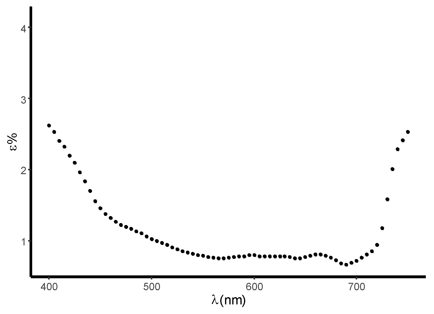
Concurrent in situ AOP measurements for 73 of the 110 inland data points shows a relatively good comparison between model derived and measured Rrs (Figure 4). Linear percentage error [28] indicates wavelength-dependent differences, introduced by the confounding effects of environmental factors, such as atmospheric variability, the water surface state (with swell-, wave-, and wavelet-induced reflections), and refraction of diffuse and direct sky and sunlight [55]. Errors are larger where the signal is smallest, e.g., below 450 nm and above 700 nm. The agreement between modelled and measured Rrs gave us confidence to use the modelled spectra to analyse spectral variability on Australian waters.
Spectral clustering resulted in 32 and 17 unique clusters for the coastal and inland waters datasets, respectively. The results of the analysis of variance test applied to the SIOP data for each cluster are listed in Table 3. The test showed that the spectral slope constant of NAP absorption coefficient (γ aNAP) contributed significantly to spectral variability within both the coastal and inland waters dataset while chlorophyll concentration contributed significantly to spectral variability within the coastal dataset and NAP concentration contributed significantly to spectral variability within the inland dataset. The absorption of CDOM at 440 nm (aCDOM(440 nm)) had a strongly significant effect on spectral variability within the coastal dataset and a lesser effect on spectral variability within the inland dataset.
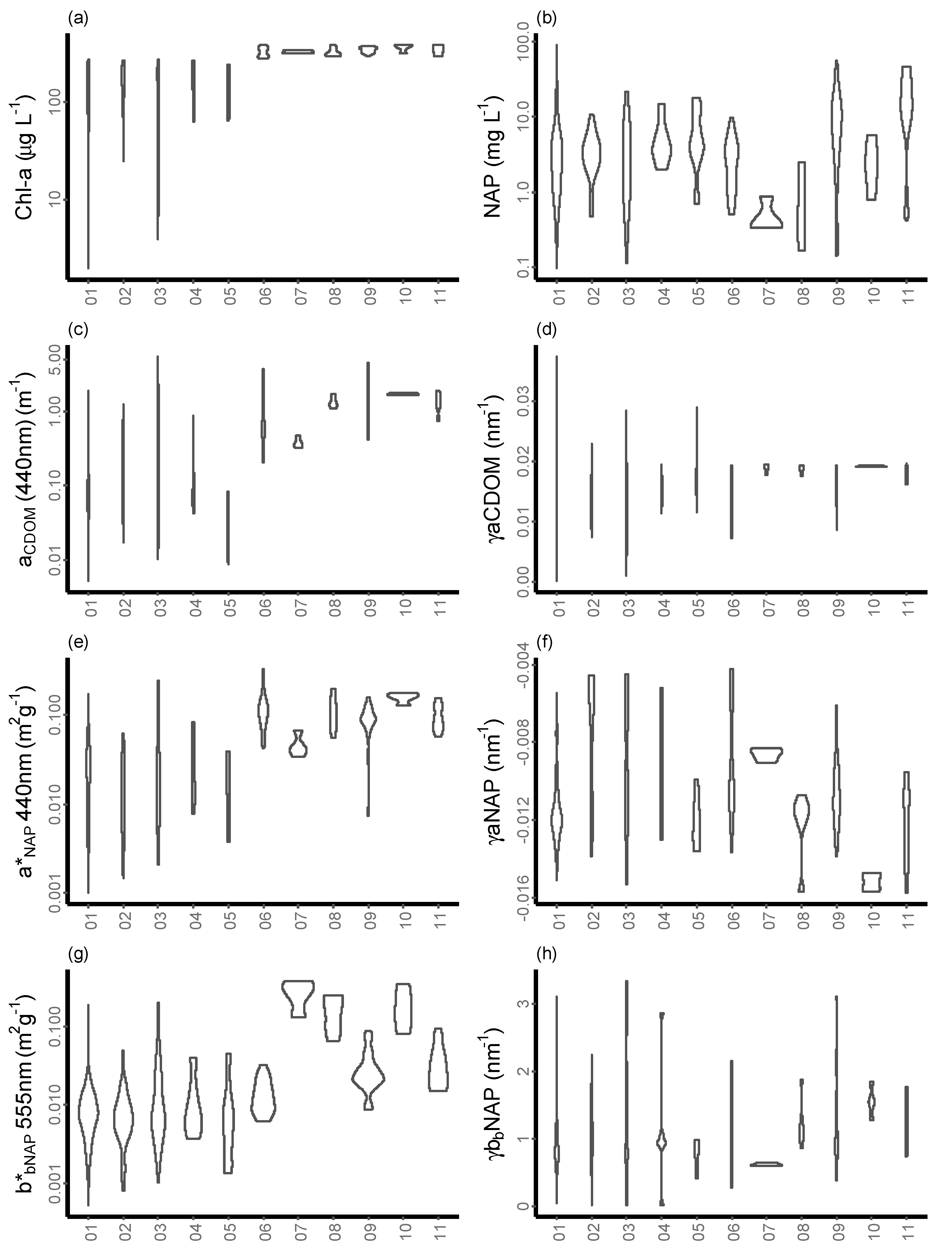
Following clustering and merging, most of the modelled spectra and modelled SIOP sets were clustered in five groups within the coastal dataset (240 of the 286 observations) and six groups within the inland dataset (102 of the 110 observations). The remaining 54 spectra represents small clusters (n < 4) or individual in situ observations that were too distinct, both spectrally and bio-optically, to be grouped with any of the bigger clusters or each other. Figure 4 shows the variability in optically active water column constituents (a–c) and SIOPs (d–h) of the 11 clusters that emerged from the data analysis. Figure 5 and Figure 6 shows the variability in the concentration, absorption and scattering characteristics of the optically active water column constituents of the 11 clusters. A summary of the main features of the 11 clusters is presented in Table 4.
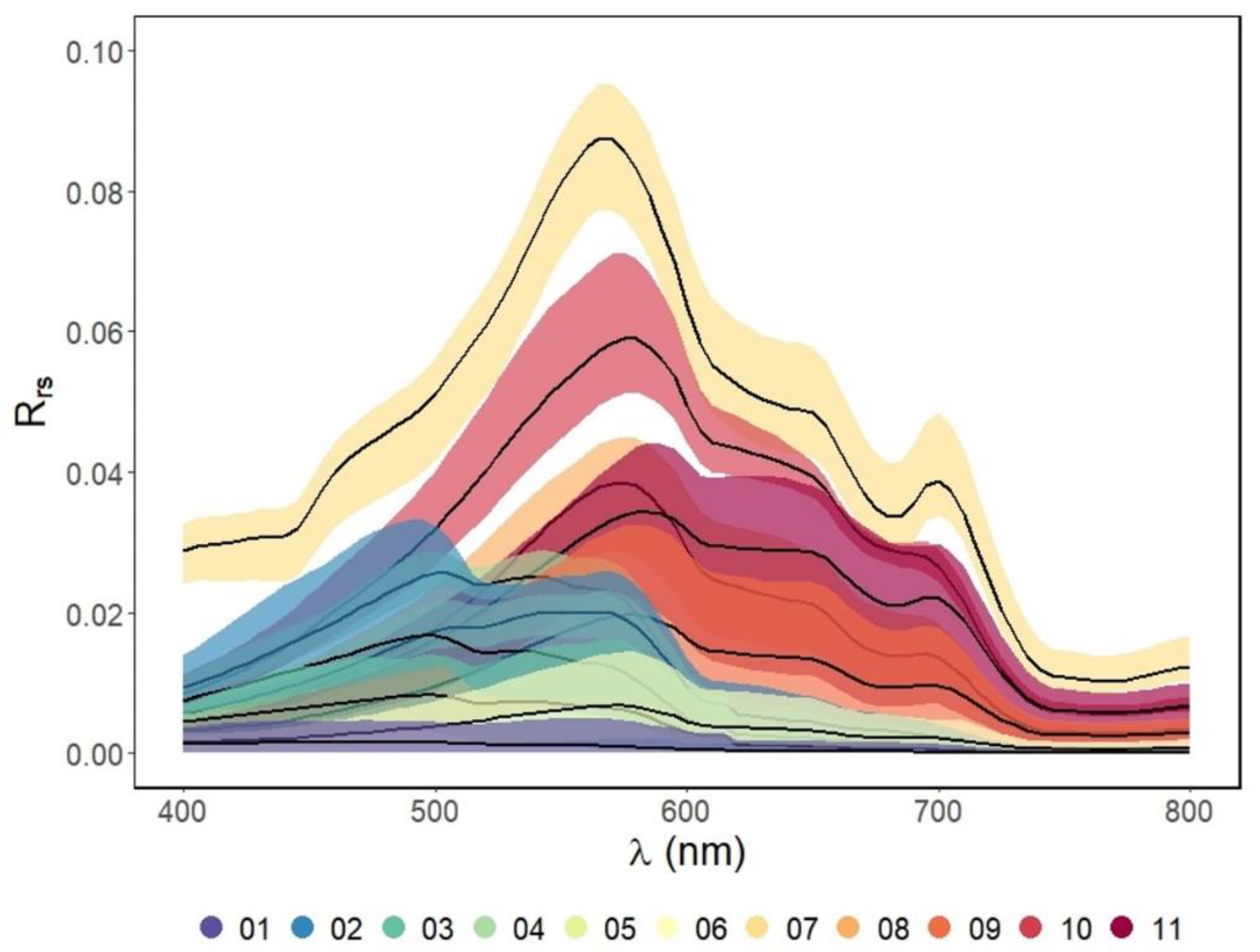
Figure 7 captures the variability in spectral shape of each of the observations that describe the 11 OWTs in the dataset. There is a clear distinction between the clusters that made up the coastal dataset (01–05) and those of the inland dataset (06–11). The coastal spectra tend to be dominated by response curves that peaks in the blue region of the spectrum while the inland spectral responses peak predominantly within the green and red region of the spectrum.
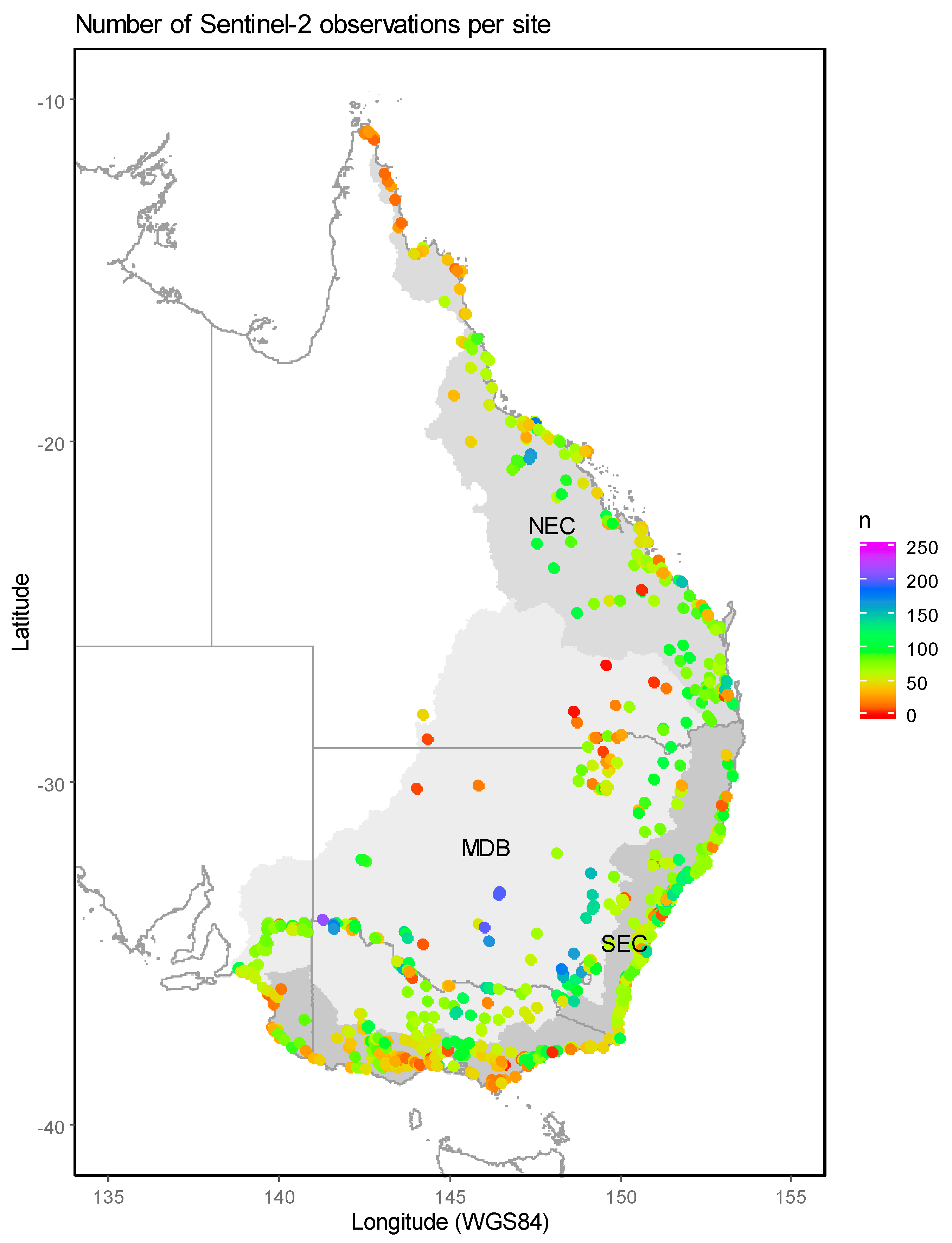
Figure 8 shows the spatial distribution of 885 locations with relatively permanent water bodies of sufficient size to not be affected by adjacency effects. The colour scale indicates the number of Sentinel-2 MSI observations retrieved from each point, while the three major drainage regions in the AOI are delineated in shades of grey. There were generally fewer observations on the western and northern sides of the MDB and in the far north of the NEC.
To determine to what extent the nSSM could match Sentinel-2 MSI surface reflectance data to the 11 OWTs, each convolved Rrs spectrum was compared to the cluster medians and ranges and assigned to the cluster that yielded the lowest nSSM metric. Ideally, the input spectra would be matched back to the original groupings that they were clustered to. However, with the reduced number of spectral bands implemented for the Sentinel-2 MSI spectra (compared to the 90 spectral bands used for the cluster analysis), some of the finer spectral differences between the clusters will be degraded. Table 5 shows an overall classification accuracy of 69% with a Kappa of 62%. Some clusters are more uniquely separable than others (e.g., 11). A few of the clusters with smaller sample sizes are more often mis-classified (e.g., 05, 07, 08, and 10). It should be noted that 08, 07, and 10 are comprised of smaller clusters that were bio-optically similar, thus compromising the spectral uniqueness of the groupings. Within the clusters with a higher number of observations, generally data belonging to the coastal dataset is most often misclassified into another coastal OWT. OWT 06, representing deep, clear inland lakes is often confused with coastal clusters, representing clear coastal waters. Cluster 09 appears to not be spectrally unique with misclassifications into several other classes.
Of the 69% of the convolved Rrs spectra that were correctly matched to the original OWT clusters, 20% were matched with an nSSM value of 1.0 or larger. 40% of the convolved Rrs spectra that were incorrectly matched to the original OWT clusters had an nSSM value exceeding 1.0. This value was selected as the maximum threshold where matches with a larger nSSM value were considered unclassified.
The surface reflectance of the Sentinel-2 MSI pixel observations was compared to each convolved modelled spectrum in each of the 11 clusters and assigned to the cluster that yielded the lowest nSSM metric. An nSSM threshold was defined by determining the lowest nSSM where most of the modelled OWT spectra were assigned to their original cluster. Any match greater than 1.00 was considered spectrally distinct from all the existing OWTs and labelled “unclassified”.
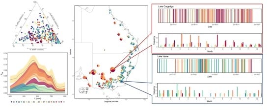
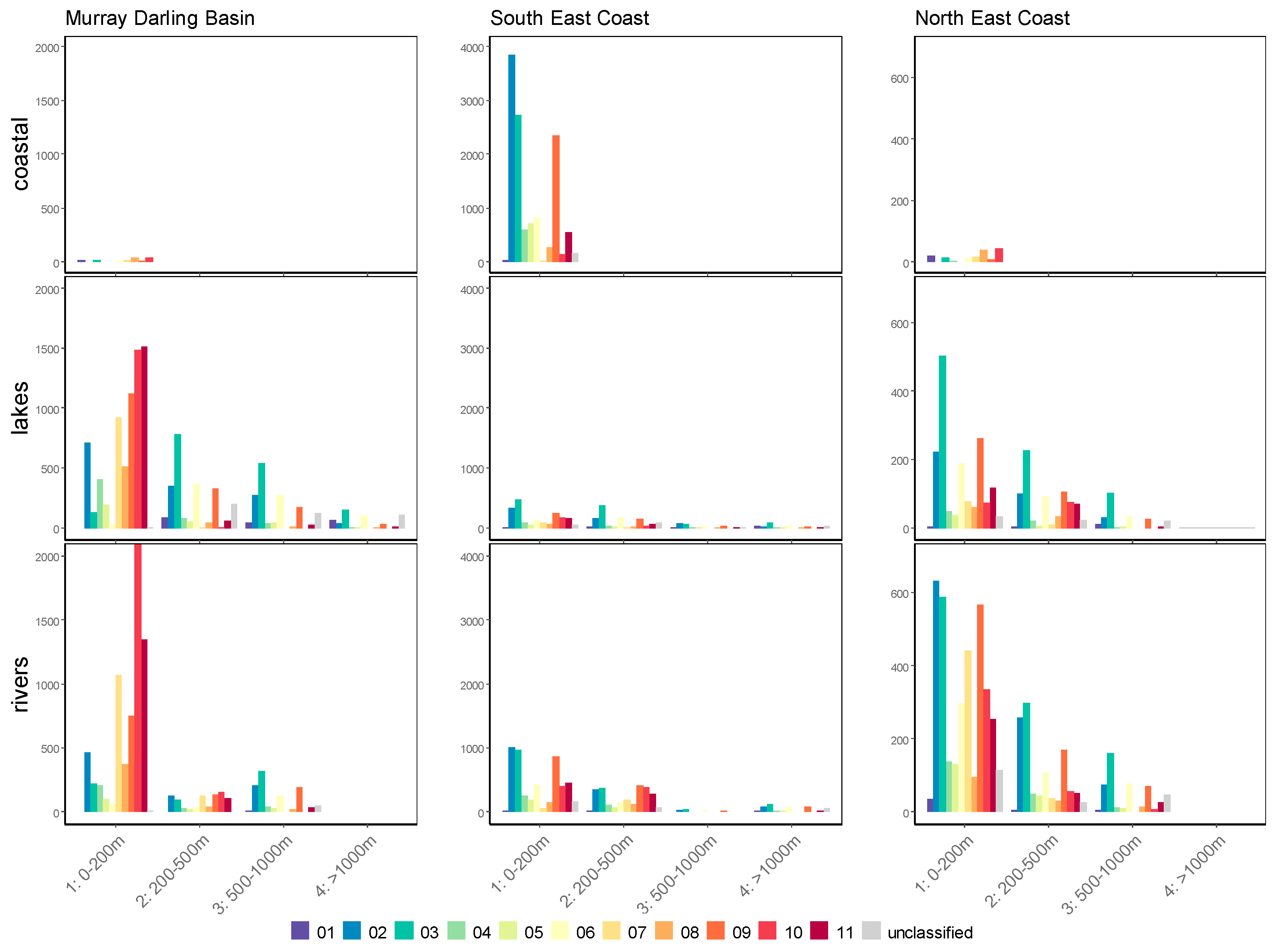
Figure 9 and Figure 10 show the limnological, landscape, and temporal distribution of OWTs matched to Sentinel-2 MSI observations over each waterbody within the three drainage regions. The observations, which were not matched with the existing OWTs, are labelled a red colour. There appear to be more unclassified observations in the inland lakes and rivers class than in the coastal waters (Figure 9).
The inland lake and river classes show a clear limnological split east and west of the Great Dividing Range (Figure 9). Waterbodies in the west (MDB) have a larger proportion of observations with dominant spectral responses in the green and red part of the spectrum and waterbodies in the east (NEC and SEC) have a higher proportion of observations with dominant spectral responses in the blue part of the spectrum.
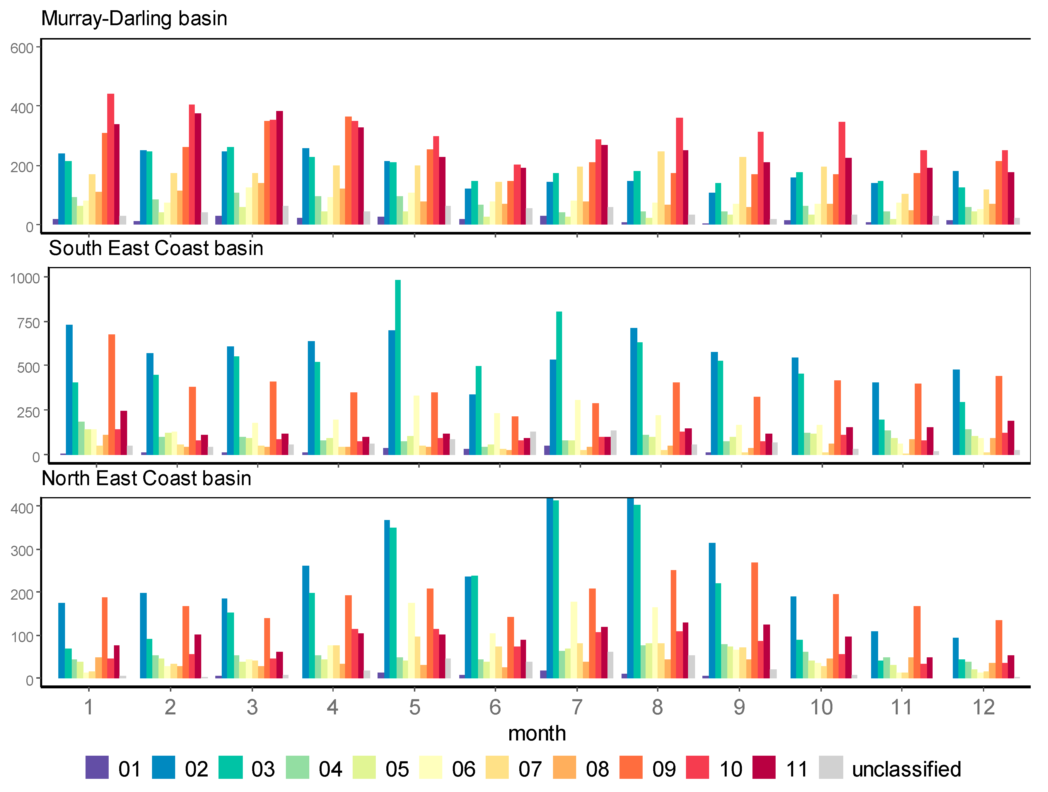
The MDB is a predominantly inland drainage basin with a wide range of climatic and geohydrological conditions (Table A3 in Appendix A). There is a strong bimodal clustering of OWTs within the lakes and rivers class in this region (Figure 9) The observations in the lakes in the lower elevations (<200m) falls predominantly in OWT classes where absorption is CDOM and NAP dominated with high amounts of suspended sediment (11) or chlorophyll (08). Lakes in higher elevations generally have clearer waters with a spectral response dominated by blue reflectance (02, 03, 06). Similarly, rivers in the lower elevations are more dominated by OWT classes with higher NAP and chlorophyll concentrations, while the higher elevations are predominantly clearer waters that are dominated by CDOM absorption (Figure 9). There appears to be a seasonal shift in water quality across the MDB drainage region with the frequency of NAP dominated OWTs decreasing during the winter months (June, July, August), and with an increase in the observation frequency of clearer OWTs during this period (Figure 10). The lake class in the higher elevations has the most unclassified observations in this drainage region.
The SEC has a temperate climate with predominantly moderate summer rainfall (Table A3), resulting in an increase in the observation frequency of more sediment dominated water types in the summer months (December, January, February, Figure 10). It has many coastal waterways, characterized by estuarine waters (Figure 9). The lakes in this region are predominantly clear while many of the rivers in the lower elevations have water that is dominated by suspended sediments (Figure 8). This region has relatively similar proportions of unclassified observations within the coastal, lake, and river classes. The rivers class in the lower elevations has the most unclassified observations within this class in this drainage region.
The monsoonal climate of the NEC (Table A3) results in a lower observation frequency in the summer months when conditions are cloudy (Figure 9). This region comprises of numerous drainage basins with predominantly natural waterways in the north. The southern drainage basins have more man-made water storages. There is also a climatological gradient with wet tropical conditions in the north and drier savannas towards the south and west. The coastal waterways in this region is characterized by estuarine waters (Figure 9). The lakes and rivers in this region are predominantly clear during the observation period while some rivers in the lower elevations have water that is dominated by suspended sediments (Figure 9). This region has relatively similar proportions of unclassified observations within the lake and river classes, while the coastal waterways have a relatively low proportion of unclassified observations.
4. Discussion
The objective of this study was to improve our knowledge of the optical complexity of Australian waters. A workflow was developed to cluster the modelled spectral response of a range of in situ bio-optical observations collected in Australian coastal and continental waters.
Coastal and inland Case 2 waters share common features and represents a continuum from fresh waters in catchments to coastal marine environments [1,2]. Despite this continuum, there is a clear distinction between the clusters that made up the coastal dataset and those of the inland dataset in this study. Similar to a global study by [1], the coastal spectra tend to be dominated by response curves that peaks in the blue region of the spectrum, while the inland spectral responses peaks predominantly within the green and red region of the spectrum.
The coastal clusters represent Australian coastal waters ranging from clear blue to more turbid estuarine waters. The first three coastal OWTs (01, 02, 03) have a strong blue reflectance signal, relative to the rest of the spectrum with absorption budgets dominated by CDOM absorption. The 01 OWT most closely resembles open ocean waters, with NAP absorption affecting the absorption budget to a small degree and very low inputs from phytoplankton. The 02 OWT represents coastal waters with a strong estuarine influence. It has the lowest γaNAP, suggesting a higher proportion of large organic particles [79,80]. The 02 OWT closely resembles the 01 OWT but has a higher phytoplankton component. The remaining two coastal OWTs (04, 05) represents moderately reflective tropical waters [49]. The 04 OWT is dominated by phytoplankton absorption and has relatively high chlorophyll content, suggesting that this represents eutrophic lagoonal waters. The higher aCDOM (440 nm) and smaller γaCDOM of the OWT indicates a coral reef matrix influence [49,81]. The higher NAP concentration and large γaNAP of the 05 OWT implies that this OWT represents tropical waters with a stronger coastal influence than 04.
The inland clusters represent eastern Australian continental waters ranging from relatively clear alpine reservoirs to turbid shallow lakes. All these OWTs have a maximum reflectance peak around 570–585 nm. The first inland OWT (06) has relatively low reflectivity and low concentrations of water column constituents, denoting clear waters with high transparency. The two green inland OWTs (07, 08) are both highly reflective water types with high chlorophyll concentrations. They are spectrally very similar with spectral differences mainly limited to a difference in the 705 nm reflectance peak and a lower reflectance in the blue region by 08, characteristic of the stronger CDOM absorption in this OWT. The 07 OWT has a smaller median γ bbNAP and a larger median γ aNAP than 08, suggesting a predominance of larger organic particles in the water column [79,80]. The last three OWTs represents waters that are dominated by NAP and CDOM absorption with a relatively small phytoplankton component. The 09 OWT has a moderate reflectivity and represents fairly clear inland waters. The comparatively high NAP absorption and low b*bNAP suggests a water column that is characterized by small suspended particles. Both the 10 and 11 OWTs are highly reflective sediment-laden water types with high NAP concentrations and high CDOM absorption. The large γaNAP of 10 suggests larger amounts of organic particulate material [79] while the relatively low b*bNAP of the 11 OWT suggests waters with smaller suspended particles [82].
To test the applicability of the 11 derived OWTs for water quality monitoring at a drainage basin scale, temporal analysis was undertaken on Sentinel-2 MSI surface reflectance observations. A total of 885 sample locations across three drainage regions were used in the case study. The satellite-derived surface reflectance observations, sourced from DEA, captured a wide range of climatological and limnological conditions. The analysis demonstrated clear limnological and seasonal differences in water types within and between the drainage divisions, which corresponds with general limnological, topographical, and climatological factors. Due to the operational period of the Sentinel-2 satellite platforms coinciding with severe drought conditions [83], there were generally fewer observations on the western and northern sides of the MDB, as surface water extents were significantly reduced. There were also fewer observations collected over this region before the Sentinel-2 platform was fully operationalized, which further confounded the analysis. Less observations in the far north of the NEC are predominantly due to cloud cover. As much of this region is subjected to monsoonal conditions in summer [84], there are larger proportions of observations made in winter, which will affect any analysis of seasonal water quality trends from satellite data in this region.
The DEA Landsat archive, representing more than 30 years of ARD observations, is ideal to capture natural water quality variations caused by seasonal, limnological, and climatological factors as well as anthropogenic factors, such as land-use change [85]. However, the atmospheric correction protocol implemented on DEA satellite data is based on standard terrestrial aerosol climatology model parameters. Atmospheric correction over water bodies is challenging because waterbodies are dark, and about 90% of the signal received by the sensor is not caused by the water itself [86,87]. The large positive bias in the shape of the reflectance in the blue bands over water targets, which is introduced by this model [73], renders the Landsat data unsuitable for the purpose of this study. With future reprocessing, incorporating a maritime aerosol type, in combination with the Landsat-8 top of atmosphere (TOA) reflectance-calibrated product and a glint-correction algorithm [73], the spectral shape of the blue bands will be more suitable for aquatic applications on DEA datasets.
Although the Sentinel-2 MSI data on DEA are corrected with the same atmospheric correction parameterization as the Landsat data, the increased number of spectral bands and finer spatial resolution somewhat alleviates the existing issues with the spectral shape of the surface reflectance spectra. To further limit the confounding effects of the existing atmospheric correction protocol on the spectral shape of aquatic targets, the coastal blue band of the Sentinel-2 MSI sensor was excluded from the analysis.
The optical cluster analysis was carried out on hyperspectral modelled Rrs spectra whilst the spectral matching of the case study was applied to five multispectral bands. The reduced spectral coverage of multispectral sensors limits the separability of water types because some water column constituents have characteristic absorption features in narrow sections of the spectrum [88]. The reduced number of spectral bands implemented for the Sentinel-2 MSI spectral analysis degraded some of the finer spectral differences between the clusters. Due to the limited spectral resolution of the Sentinel-2 satellite data, the spectral signatures of some of the OWTs in this study became less uniquely separable than others. To mitigate the confounding effect of the reduced spectral resolution of the Sentinel-2 bands, a threshold metric was defined. An optimal threshold is a compromise between maximizing the probability of a correct match and minimizing the rate of false positive matches [89]. The threshold defined for the nSSM metric balances the requirement to capture the maximum number of correct spectral matches with the need to identify areas where there are genuine gaps in the existing water quality database. To limit the confounding effect of environmental factors on the accuracy of results, care was taken to select only observations that were not affected by atmospheric variability, sun glint, and the effects of the brighter response of adjacent terrestrial targets [56].
The OWT classification of waterbodies demonstrates clear limnological and seasonal differences in water types within and between the drainage divisions, which corresponds with general limnological, topographical, and climatological factors in those regions [84]. Unclassified observations were clustered predominantly in lakes within the alpine regions and east of the Great Dividing Range. Observations within rivers (flowing water) are less frequently labelled unclassified. Targets with a higher albedo were more often matched to an OWT, suggesting that some of the unclassified observations in the deep, clear lakes in the alpine regions [84] may be due to low target albedo. The water leaving signal at the satellite sensor is a small part of the total measured signal [86,88]; this potentially constrains the ability of the Sentinel-2 sensor to record a sufficient amount of water leaving light through a set of atmospheric and air water interface conditions to allow a clearly distinguishable spectral signature that can be matched to an existing OWT.
5. Conclusions
The OWTs defined in this study were based on in situ observations capturing the bio-optical response of a wide range seasonal and geographical variability. The extent of the Australian coastline and diversity of continental landscape and climatic features implies that there may still be gaps in our knowledge. For example, the current coastal dataset, except for the Great Barrier Reef, lacks the temporal range to fully understand the variability associated with seasons [90]. Similarly, the inland dataset has been sourced exclusively from eastern Australia and lacks data associated with unique limnological features further west [91].
The deficiency in capturing the full variability of water quality across the Australian landscape can be observed in the clustering of waterbodies that regularly do not match to any of the existing OWTs in the study area of the case study. The locations of the unclassified observations can be used to inform where investment for in situ bio-optical data acquisition may be better targeted to achieve a more comprehensive objective characterization of all Australian waters, which can contribute to global initiatives like the SDG.
Supplementary Materials
The following are available online at https://www.mdpi.com/2072-4292/12/18/3018/s1, Table S1: Description of the coastal and marine datasets used in this work, Table S2: Description of the lakes and reservoirs that contributed towards the inland water quality dataset, Figure S1: Hierarchical clustering dendrogram of the simulated Rrs spectra produced from the coastal waters dataset, Figure S2: Hierarchical clustering dendrogram of the simulated Rrs spectra produced from the inland waters dataset.
Author Contributions
Conceptualization, E.J.B.; data curation, E.J.B. and T.A.G.M.; formal analysis, E.J.B.; funding acquisition, J.M.A. and S.S.; investigation, E.J.B.; methodology, E.J.B. and E.L.; project administration, J.M.A. and S.S.; resources, S.S. and T.A.G.M.; software, E.L.; supervision, J.M.A.; validation, E.J.B.; visualization, E.J.B.; writing—original draft, E.J.B.; writing—review & editing, E.J.B., J.M.A., S.S., E.L. and T.A.G.M. All authors have read and agreed to the published version of the manuscript.
Funding
IWQual—a collaborative project between CSIRO and Geoscience Australia.
Acknowledgments
The authors wish to acknowledge and thank the many CSIRO staff, past and present, involved in the acquisition of the data that underpins our science. For each of these many field campaigns, Lesley Clementson (CSIRO Oceans and Atmosphere, Hobart) has undertaken the laboratory analyses of constituent concentrations, absorptions, pigment data and is gratefully acknowledged.
Conflicts of Interest
The authors declare no conflict of interest.
Appendix A
Table A1.
Glossary of acronyms used in this manuscript.
| Acronym | Description |
|---|---|
| AOI | Area of Interest |
| ARD | Analysis ready data |
| DEA | Digital Earth Australia |
| ED | Euclidian Distance |
| EO | Earth Observation |
| FCM | Fuzzy-c Means |
| GIOP | Generalized Inherent Optical Properties |
| IOP | Inherent Optical Properties |
| IOSODATA | Iterative Self-Organizing Data Analysis Techniques |
| Kd | Vertical Attenuations |
| MDB | Murray-Darling Basin |
| NAP | Non-algal particulates |
| NCI | National Computing Infrastructure |
| NEC | North East Coastal |
| nSSM | normalized Spectral Similarity Metric |
| ODC | Open Data Cube |
| OWT | Optical Water Types |
| Rrs | Remote Sensing reflectance |
| rrs | Subsurface reflectance |
| SDG | Sustainable Development Goals |
| SDz | Secchi Depth |
| SEC | South East Coastal |
| SIOP | Specific Inherent Optical Properties |
| TOA | Top of Atmosphere |
| TSS | Total Suspended Solids |
| WFCM | Weighted Fuzzy-c Means |
| WOfS | Water Observations from Space |
Table A2.
Glossary of water column constituents presented in this study.
| Parameter | Description | Unit |
|---|---|---|
| CCHL | Chlorophyll concentration (a proxy for phytoplankton) | μg L−1 |
| CDOM | Coloured dissolved organic matter | |
| CNAP | Non algal particulates concentration | mg L−1 |
| PHY | Phytoplankton | |
| a*PHY(440 nm) | Chlorophyll-a specific absorption at 440 nm | m2mg−1 |
| a*PHY(676 nm) | Chlorophyll-a specific absorption at 676 nm | m2mg−1 |
| γ aCDOM | Spectral slope constant of CDOM absorption coefficient | nm−1 |
| aCDOM(440 nm) | Absorption of CDOM at 440 nm | m−1 |
| a*NAP(440 nm) | Specific absorption of NAP at 440 nm | m2g−1 |
| γ aNAP | Spectral slope constant of NAP absorption coefficient | nm−1 |
| b*bNAP(555 nm) | Specific backscattering due to NAP at 555 nm | m2g−1 |
| γ bbNAP | Spectral slope constant of NAP backscattering coefficient | nm−1 |
Table A3.
Summary of the main characteristics of the three drainage regions in Eastern Australia used as the area of interest (AOI) of the case study.
Table A3.
Summary of the main characteristics of the three drainage regions in Eastern Australia used as the area of interest (AOI) of the case study.
| Basin | Area (km2) | Mean Rainfall (mm) | Mean Elevation (m) | Climate | Hydrogeology | Land Use |
|---|---|---|---|---|---|---|
| MDB | 1,061,000 | 458 | 260 | Range of climatic conditions: cool and humid eastern uplands; temperate southeast; subtropical northeast with monsoonal rain; hot, dry semi-arid; arid western plains. | Basinal aquifers in sedimentary deposits within the flatter landscapes; fractured rock aquifers and valley-fill alluvium in the highlands bordering the basin. | Dryland pasture, dryland and irrigated cropping, and urban land use. |
| NEC | 451,000 | 827 | 173 | Subtropical to tropical with hot, wet summers and cooler, dry winters. Monsoonal summer rainfall in the north, winter rainfall the south. | Topographically diverse terrain with high relief in coastal ranges and tablelands and coastal alluvial plains. Outcropping fractured basement rock, alluvial valley systems, and coastal sand deposits. | Native pasture, dryland and irrigated agriculture, and urban land use. |
| SEC | 129,500 | 995 | 323 | Warm temperate climate with moderate rainfall. | Outcropping fractured basement rock, alluvial valley, and coastal sand aquifers. | Nature conservation, dryland pasture, irrigated and dryland cropping, and urban land use |
References
- Spyrakos, E.; O’Donnell, R.; Hunter, P.D.; Miller, C.; Scott, M.; Simis, S.G.H.; Neil, C.; Barbosa, C.C.F.; Binding, C.E.; Bradt, S.; et al. Optical types of inland and coastal waters. Limnol. Oceanogr. 2018, 63, 846–870. [Google Scholar] [CrossRef] [Green Version]
- Tyler, A.N.; Hunter, P.D.; Spyrakos, E.; Groom, S.; Constantinescu, A.M.; Kitchen, J. Developments in earth observation for the assessment and monitoring of inland, transitional, coastal and shelf-sea waters. Sci. Total Environ. 2016, 572, 1307–1321. [Google Scholar] [CrossRef] [Green Version]
- Argent, R.M. Australia State of The Environment 2016: Inland Water, Independent Report to the Australian Government Minister for the Environment and Energy; Australian Government Department of the Environment and Energy: Canberra, Australia, 2017. [CrossRef]
- Dekker, A.G.; Hestir, E.L. Evaluating the Feasibility of Systematic Inland Water Quality Monitoring with Satellite Remote Sensing; CSIRO Water for a Healthy Country National Research Flagship: Canberra, Australia, 2012. [Google Scholar] [CrossRef]
- Malthus, T.J.; Hestir, E.L.; Dekker, A.G.; Brando, V.E. The case for a global inland water quality product. In Proceedings of the 2012 IEEE International Geoscience and Remote Sensing Symposium, Munich, Germany, 22–27 July 2012; pp. 5234–5237. [Google Scholar] [CrossRef]
- Matthews, M.W. A current review of empirical procedures of remote sensing in inland and near-coastal transitional waters. Int. J. Remote Sens. 2010, 32, 6855–6899. [Google Scholar] [CrossRef]
- Bonansea, M.; Rodriguez, M.C.; Pinotti, L.; Ferrero, S. Using multi-temporal Landsat imagery and linear mixed models for assessing water quality parameters in Rio Tercero reservoir (Aargentina). Remote Sens. Environ. 2015, 158, 28–41. [Google Scholar] [CrossRef]
- Torbick, N.; Hession, S.; Hagen, S.; Wiangwang, N.; Becker, B.; Qi, J.G. Mapping inland lake water quality across the lower peninsula of Michigan using Landsat TM imagery. Int. J. Remote Sens. 2013, 34, 7607–7624. [Google Scholar] [CrossRef]
- Brezonik, P.; Menken, K.D.; Bauer, M. Landsat-based remote sensing of lake water quality characteristics, including chlorophyll and colored dissolved organic matter (CDOM). Lake Reserv. Manag. 2005, 21, 373–382. [Google Scholar] [CrossRef]
- Dekker, A.G.; Vos, R.J.; Peters, S.W.M. Analytical algorithms for lake water TSM estimation for retrospective analyses of TM and SPOT sensor data. Int. J. Remote Sens. 2002, 23, 15–35. [Google Scholar] [CrossRef]
- Lymburner, L.; Botha, E.; Hestir, E.; Anstee, J.; Sagar, S.; Dekker, A.; Malthus, T. Landsat 8: Providing continuity and increased precision for measuring multi-decadal time series of total suspended matter. Remote Sens. Environ. 2016, 185, 108–118. [Google Scholar] [CrossRef]
- Hellweger, F.L.; Schlosser, P.; Lall, U.; Weissel, J.K. Use of satellite imagery for water quality studies in New York harbor. Estuar. Coast. Shelf Sci. 2004, 61, 437–448. [Google Scholar] [CrossRef]
- Hadjimitsis, D.G.; Hadjimitsis, M.G.; Clayton, C.; Clarke, B.A. Determination of turbidity in Kourris dam in Cyprus utilizing Landsat TM remotely sensed data. Water Resour. Manag. 2006, 20, 449–465. [Google Scholar] [CrossRef]
- Lehmann, M.K.; Nguyen, U.; Allan, M.; van der Woerd, H.J. Colour classification of 1486 lakes across a wide range of optical water types. Remote Sens. 2018, 10, 1273. [Google Scholar] [CrossRef] [Green Version]
- Van der Woerd, H.J.; Wernand, M.R. True colour classification of natural waters with medium-spectral resolution satellites: SeaWIFS, MODIS, MERIS and OLCI. Sensors 2015, 15, 25663–25680. [Google Scholar] [CrossRef] [PubMed] [Green Version]
- Wang, S.; Lee, Z.; Shang, S.; Li, J.; Zhang, B.; Lin, G. Deriving inherent optical properties from classical water color measurements: Forel-Ule index and secchi disk depth. Opt. Express 2019, 27, 7642–7655. [Google Scholar] [CrossRef]
- Bugnot, A.B.; Lyons, M.B.; Scanes, P.; Clark, G.F.; Fyfe, S.K.; Lewis, A.; Johnston, E.L. A novel framework for the use of remote sensing for monitoring catchments at continental scales. J. Environ. Manag. 2018, 217, 939–950. [Google Scholar] [CrossRef]
- Heege, T.; Kiselev, V.; Wettle, M.; Hung, N.N. Operational multi-sensor monitoring of turbidity for the entire Mekong delta. Int. J. Remote Sens. 2014, 35, 2910–2926. [Google Scholar] [CrossRef]
- Olmanson, L.G.; Bauer, M.E.; Brezonik, P.L. A 20-year Landsat water clarity census of Minnesota’s 10,000 lakes. Remote Sens. Environ. 2008, 112, 4086–4097. [Google Scholar] [CrossRef]
- Lobo, F.L.; Costa, M.P.F.; Novo, E. Time-series analysis of Landsat-MSS/TM/OLI images over Amazonian waters impacted by gold mining activities. Remote Sens. Environ. 2015, 157, 170–184. [Google Scholar] [CrossRef]
- Bowling, L.; Baldwin, D.; Merrick, C.; Brayan, J.; Panther, J. Possible drivers of a chrysosporum ovalisporum bloom in the Murray River, Australia, in 2016. Mar. Freshw. Res. 2018, 69, 1649–1662. [Google Scholar] [CrossRef] [Green Version]
- Siegel, D.A.; Maritorena, S.; Nelson, N.B.; Behrenfeld, M.J.; McClain, C.R. Colored dissolved organic matter and its influence on the satellite-based characterization of the ocean biosphere. Geophys. Res. Lett. 2005, 32. [Google Scholar] [CrossRef] [Green Version]
- Dierssen, H.M.; Smith, R.C. Bio-optical properties and remote sensing ocean color algorithms for Antarctic peninsula waters. J. Geophys. Res. Ocean. 2000, 105, 26301–26312. [Google Scholar] [CrossRef]
- Otero, M.P.; Siegel, D.A. Spatial and temporal characteristics of sediment plumes and phytoplankton blooms in the Santa Barbara channel. Deep-Sea Res. Part II Top. Stud. Oceanogr. 2004, 51, 1129–1149. [Google Scholar] [CrossRef]
- Feng, H.; Campbell, J.W.; Dowell, M.D.; Moore, T.S. Modeling spectral reflectance of optically complex waters using bio-optical measurements from Tokyo bay. Remote Sens. Environ. 2005, 99, 232–243. [Google Scholar] [CrossRef]
- Santini, F.; Alberotanza, L.; Cavalli, R.M.; Pignatti, S. A two-step optimization procedure for assessing water constituent concentrations by hyperspectral remote sensing techniques: An application to the highly turbid Venice lagoon waters. Remote Sens. Environ. 2010, 114, 887–898. [Google Scholar] [CrossRef]
- Heege, T.F.J. Mapping of water constituents in Lake Constance using multispectral airborne scanner data and a physically based processing scheme. Can. J. Remote Sens. 2004, 30, 77–86. [Google Scholar] [CrossRef]
- Lee, Z.; Carder, K.L.; Arnone, R.A. Deriving inherent optical properties from water color: A multiband quasi-analytical algorithm for optically deep waters. Appl. Opt. 2002, 41, 5755–5772. [Google Scholar] [CrossRef]
- Brando, V.E.; Anstee, J.M.; Wettle, M.; Dekker, A.G.; Phinn, S.R.; Roelfsema, C. A physics based retrieval and quality assessment of bathymetry from suboptimal hyperspectral data. Remote Sens. Environ. 2009, 113, 755–770. [Google Scholar] [CrossRef]
- Brando, V.E.; Dekker, A.G.; Park, Y.J.; Schroeder, T. Adaptive semianalytical inversion of ocean color radiometry in optically complex waters. Appl. Opt. 2012, 51, 2808–2833. [Google Scholar] [CrossRef]
- Melin, F.; Vantrepotte, V.; Clerici, M.; D’Alimonte, D.; Zibordi, G.; Berthon, J.F.; Canuti, E. Multi-sensor satellite time series of optical properties and chlorophyll-a concentration in the Adriatic Sea. Prog. Oceanogr. 2011, 91, 229–244. [Google Scholar] [CrossRef]
- Shanmugam, P. A new bio-optical algorithm for the remote sensing of algal blooms in complex ocean waters. J. Geophys. Res. Ocean. 2011, 116, 12. [Google Scholar] [CrossRef] [Green Version]
- Vantrepotte, V.; Loisel, H.; Dessailly, D.; Meriaux, X. Optical classification of contrasted coastal waters. Remote Sens. Environ. 2012, 123, 306–323. [Google Scholar] [CrossRef]
- McKee, D.; Cunningham, A. Identification and characterisation of two optical water types in the Irish Sea from in situ inherent optical properties and seawater constituents. Estuar. Coast. Shelf Sci. 2006, 68, 305–316. [Google Scholar] [CrossRef]
- Spyrakos, E.; Vilas, L.G.; Palenzuela, J.M.T.; Barton, E.D. Remote sensing chlorophyll a of optically complex waters (Rias Baixas, NW Spain): Application of a regionally specific chlorophyll a algorithm for MERIS full resolution data during an upwelling cycle. Remote Sens. Environ. 2011, 115, 2471–2485. [Google Scholar] [CrossRef] [Green Version]
- Dzwonkowski, B.; Yan, X.H. Development and application of a neural network based ocean colour algorithm in coastal waters. Int. J. Remote Sens. 2005, 26, 1175–1200. [Google Scholar] [CrossRef]
- Lubac, B.; Loisel, H. Variability and classification of remote sensing reflectance spectra in the eastern English Channel and southern North Sea. Remote Sens. Environ. 2007, 110, 45–58. [Google Scholar] [CrossRef]
- IOCCG. Remote Sensing of Ocean Colour in Coastal, and Other Optically-Complex, Waters; IOCCG: Dartmouth, Canada, 2000. [Google Scholar] [CrossRef]
- Morel, A.; Prieur, L. Analysis of variations in ocean color. Limnol. Oceanogr. 1977, 22, 709–722. [Google Scholar] [CrossRef]
- Zibordi, G.; Holben, B.; Slutsker, I.; Giles, D.; D’Alimonte, D.; Melin, F.; Berthon, J.F.; Vandemark, D.; Feng, H.; Schuster, G.; et al. AERONET-OC: A network for the validation of ocean color primary products. J. Atmos. Ocean. Technol. 2009, 26, 1634–1651. [Google Scholar] [CrossRef]
- Zibordi, G.; Berthon, J.F.; Melin, F.; D’Alimonte, D. Cross-site consistent in situ measurements for satellite ocean color applications: The bioMap radiometric dataset. Remote Sens. Environ. 2011, 115, 2104–2115. [Google Scholar] [CrossRef]
- Traykovski, L.V.M.; Sosik, H.M. Feature-based classification of optical water types in the northwest Atlantic based on satellite ocean color data. J. Geophys. Res. Ocean. 2003, 108, 18. [Google Scholar] [CrossRef] [Green Version]
- Melin, F.; Vantrepotte, V. How optically diverse is the coastal ocean? Remote Sens. Environ. 2015, 160, 235–251. [Google Scholar] [CrossRef]
- Moore, T.S.; Dowell, M.D.; Bradt, S.; Verdu, A.R. An optical water type framework for selecting and blending retrievals from bio-optical algorithms in lakes and coastal waters. Remote Sens. Environ. 2014, 143, 97–111. [Google Scholar] [CrossRef] [Green Version]
- Shen, Q.; Li, J.S.; Zhang, F.F.; Sun, X.; Li, J.; Li, W.; Zhang, B. Classification of several optically complex waters in China using in situ remote sensing reflectance. Remote Sens. 2015, 7, 14731–14756. [Google Scholar] [CrossRef] [Green Version]
- Eleveld, M.A.; Ruescas, A.B.; Hommersom, A.; Moore, T.S.; Peters, S.W.M.; Brockmann, C. An optical classification tool for global lake waters. Remote Sens. 2017, 9, 24. [Google Scholar] [CrossRef] [Green Version]
- Ye, H.P.; Li, J.S.; Li, T.J.; Shen, Q.; Zhu, J.H.; Wang, X.Y.; Zhang, F.F.; Zhang, J.; Zhang, B. Spectral classification of the Yellow Sea and implications for coastal ocean color remote sensing. Remote Sens. 2016, 8, 23. [Google Scholar] [CrossRef] [Green Version]
- Reinart, A.; Herlevi, A.; Arst, H.; Sipelgas, L. Preliminary optical classification of lakes and coastal waters in Estonia and south Finland. J. Sea Res. 2003, 49, 357–366. [Google Scholar] [CrossRef]
- Blondeau-Patissier, D.; Brando, V.; Oubelkheir, K.; Dekker, A.; Clementson, L.; Daniel, P. Bio-optical variability of the absorption and scattering properties of the Queensland inshore and reef waters, Australia. J. Geophys. Res. Ocean. 2009, 114, 24. [Google Scholar] [CrossRef]
- Brando, V.E.; Blondeau-Patissier, D.; Dekker, A.G.; Daniel, P.J.; Wettle, M.; Oubelkheir, K.; Clementson, L. Bio-optical variability of Queensland coastal waters for parameterisation of coastal-reef algorithms. In Proceedings of the Ocean Optics XVIII, ONR-NASA, Montreal, QC, Canada, 9–13 October 2006. [Google Scholar] [CrossRef]
- Cherukuru, N.; Brando, V.; Schroeder, T.; Clementson, L.; Dekker, A. Influence of river discharge and ocean currents on coastal optical properties. Cont. Shelf Res. 2014, 84, 188–203. [Google Scholar] [CrossRef]
- Thompson, P.; Bonham, P.; Waite, A.; Clementson, L.; Cherukuru, N.; Hassler, C.; Doblin, M. Contrasting oceanographic conditions and phytoplankton communities on the east and west coasts of Australia. Deep-Sea Res. Part II Top. Stud. Oceanogr. 2011, 58, 645–663. [Google Scholar] [CrossRef]
- Hestir, E.L.; Brando, V.; Campbell, G.; Dekker, A.; Malthus, T. The relationship between dissolved organic matter absorption and dissolved organic carbon in reservoirs along a temperate to tropical gradient. Remote Sens. Environ. 2015, 156, 395–402. [Google Scholar] [CrossRef]
- Clementson, L.A.; Parslow, J.S.; Turnbull, A.R.; McKenzie, D.C.; Rathbone, C.E. Optical properties of waters in the Australasian sector of the Southern Ocean. J. Geophys. Res. 2001, 106, 31611–31625. [Google Scholar] [CrossRef]
- Brando, V.E.; Dekker, A.G. Satellite hyperspectral remote sensing for estimating estuarine and coastal water quality. IEEE Trans.Geosci. Remote Sens. 2003, 41, 1378–1387. [Google Scholar] [CrossRef]
- Botha, E.J.; Brando, V.E.; Dekker, A.G. Effects of per-pixel variability on uncertainties in bathymetric retrievals from high-resolution satellite images. Remote Sens. 2016, 8, 18. [Google Scholar] [CrossRef] [Green Version]
- Ruddick, K.G.; Voss, K.; Boss, E.; Castagna, A.; Frouin, R.; Gilerson, A.; Hieronymi, M.; Johnson, B.C.; Kuusk, J.; Lee, Z.; et al. A review of protocols for fiducial reference measurements of water-leaving radiance for validation of satellite remote-sensing data over water. Remote Sens. 2019, 11, 2198. [Google Scholar] [CrossRef] [Green Version]
- Torrecilla, E.; Stramski, D.; Reynolds, R.A.; Millan-Nunez, E.; Piera, J. Cluster analysis of hyperspectral optical data for discriminating phytoplankton pigment assemblages in the open ocean. Remote Sens. Environ. 2011, 115, 2578–2593. [Google Scholar] [CrossRef] [Green Version]
- Mobley, C.D. Hydrolight 3.0 Users’ Guide—Final Report—March 1995; SRI Project 5632, Contract N00014-94-C-0062; SRI International: Menlo Park, CA, USA, 1995. [Google Scholar]
- Mobley, C.D. Light and Water; Radiative Transfer in Natural Waters; Academic Press: London, UK, 1994. [Google Scholar]
- Jain, A.K.; Murty, M.N.; Flynn, P.J. Data clustering: A review. ACM Comput. Surv. 1999, 31, 264–323. [Google Scholar] [CrossRef]
- Ward, J.H. Hierarchical grouping to optimize an objective function. J. Am. Stat. Assoc. 1963, 58, 236–244. [Google Scholar] [CrossRef]
- Murtagh, F.; Contreras, P. Algorithms for hierarchical clustering: An overview, II. Wiley Interdiscip. Rev. Data Min. Knowl. Discov. 2017, 7, 16. [Google Scholar] [CrossRef] [Green Version]
- Benjamini, Y.; Braun, H.; John, W. Tukey’s contributions to multiple comparisons. Ann. Stat. 2002, 30, 1576–1594. [Google Scholar] [CrossRef]
- Wilson, C.O. Land use/land cover water quality nexus: Quantifying anthropogenic influences on surface water quality. Environ. Monit. Assess. 2015, 187. [Google Scholar] [CrossRef]
- Killough, B. Overview of the Open Data Cube Initiative. In 2018 IEEE International Geoscience and Remote Sensing Symposium; IEEE: New York, NY, USA, 2018; pp. 8629–8632. [Google Scholar] [CrossRef]
- Loveland, T.R.; Dwyer, J.L. Landsat: Building a strong future. Remote Sens. Environ. 2012, 122, 22–29. [Google Scholar] [CrossRef]
- Lewis, A.; Oliver, S.; Lymburner, L.; Evans, B.; Wyborn, L.; Mueller, N.; Raevski, G.; Hooke, J.; Woodcock, R.; Sixsmith, J.; et al. The Australian Geoscience Data Cube—Foundations and lessons learned. Remote Sens. Environ. 2017, 202, 276–292. [Google Scholar] [CrossRef]
- Li, F.Q.; Jupp, D.L.B.; Reddy, S.; Lymburner, L.; Mueller, N.; Tan, P.; Islam, A. An evaluation of the use of atmospheric and BRDF correction to standardize Landsat data. IEEE J. Sel. Toppics Appl. Earth Obs. Remote Sens. 2010, 3, 257–270. [Google Scholar] [CrossRef]
- Sixsmith, J.; Oliver, S.; Lymburner, L. IEEE A hybrid approach to automated Landsat pixel quality. In 2013 IEEE International Geoscience and Remote Sensing Symposium; IEEE: New York, NY, USA, 2013; pp. 4146–4149. [Google Scholar] [CrossRef]
- Irish, R.R.; Barker, J.L.; Goward, S.N.; Arvidson, T. Characterization of the Landsat-7 ETM+ automated cloud-cover assessment (ACCA) algorithm. Photogramm. Eng. Remote Sens. 2006, 72, 1179–1188. [Google Scholar] [CrossRef]
- Zhu, Z.; Woodcock, C.E. Object-based cloud and cloud shadow detection in Landsat imagery. Remote Sens. Environ. 2012, 118, 83–94. [Google Scholar] [CrossRef]
- Schroeder, T. Aquatic Atmospheric Correction—Aerosol Ancillary Data and Product Validation, Data Analysis Report, Prepared for Geoscience Australia; EP194931; CSIRO Oceans and Atmosphere: Canberra, Australia, 2019; p. 71. [Google Scholar]
- Mueller, N.; Lewis, A.; Roberts, D.; Ring, S.; Melrose, R.; Sixsmith, J.; Lymburner, L.; McIntyre, A.; Tan, P.; Curnow, S.; et al. Water observations from space: Mapping surface water from 25 years of Landsat imagery across Australia. Remote Sens. Environ. 2016, 174, 341–352. [Google Scholar] [CrossRef] [Green Version]
- Vanhellemont, Q.; Ruddick, K. Advantages of high quality SWIR bands for ocean colour processing: Examples from Landsat-8. Remote Sens. Environ. 2015, 161, 89–106. [Google Scholar] [CrossRef] [Green Version]
- Dyall, A.; Heap, A.D.; Tobin, G.; Bryce, S.; Ryan, D.A.; Galinec, V.; Creasey, J.; Gallagher, J.; Radke, L.; Smith, C.; et al. Australian Coastal Waterways Geomorphic Habitat Mapping (National Aggregated Product); Geoscience Australia: Canberra, Australia, 2005. Available online: http://metadata.imas.utas.edu.au/geonetwork/srv/en/metadata.show?uuid=9b403526-e386-47ef-8a78-be1ae179419d (accessed on 8 September 2019).
- Geoscience Australia. Geodata Topo 2.5 m 2003, 3rd ed.; Geoscience Australia: Canberra, Australia, 2003. Available online: http://pid.geoscience.gov.au/dataset/ga/60804 (accessed on 8 September 2019).
- Botha, E.J.; Brando, V.; Dekker, A.; Anstee, J.M.; Sagar, S. Increased spectral resolution enhances coral detection under varying water conditions. Remote Sens. Environ. 2013, 131, 247–261. [Google Scholar] [CrossRef]
- Babin, M.; Stramski, D.; Ferrari, G.M.; Claustre, H.; Bricaud, A.; Obolensky, G.; Hoepffner, N. Variations in the light absorption coefficients of phytoplankton, nonalgal particles, and dissolved organic matter in coastal waters around Europe. J. Geophys. Res. 2003, 108. [Google Scholar] [CrossRef]
- Slade, W.H.; Boss, E. Spectral attenuation and backscattering as indicators of average particle size. Appl. Opt. 2015, 54, 7264–7277. [Google Scholar] [CrossRef]
- Zanardi-Lamardo, E.; Moore, C.; Zika, R. Seasonal variation in molecular mass and optical properties of chromophoric dissolved organic material in coastal waters of southwest Florida. Mar. Chem. 2004, 89, 37–54. [Google Scholar] [CrossRef]
- Shi, K.; Li, Y.M.; Li, L.; Lu, H. Absorption characteristics of optically complex inland waters: Implications for water optical classification. J. Geophys. Res. Biogeosci. 2013, 118, 860–874. [Google Scholar] [CrossRef]
- Australian Bureau of Meteorology. Special Climate Statement 70—Drought Conditions in Australia and Impact on Water Resources in the Murray–Darling Basin; Australian Bureau of Meteorology: Melbourne, Australia, 2019. Available online: http://www.bom.gov.au/climate/current/statements/scs70.pdf (accessed on 12 September 2019).
- Australian Bureau of Meteorology. Australian Water Resources Assessment 2010; Bureau of Meteorology: Melbourne, Australia, 2011. Available online: http://www.bom.gov.au/water/awra/2010/documents/assessment-low.pdf on (accessed on 12 September 2019).
- Lewis, A.; Lymburner, L.; Purss, M.B.J.; Brooke, B.; Evans, B.; Ip, A.; Dekker, A.G.; Irons, J.R.; Minchin, S.; Mueller, N.; et al. Rapid, high-resolution detection of environmental change over continental scales from satellite data—The earth observation data cube. Int. J. Digit. Earth 2016, 9, 106–111. [Google Scholar] [CrossRef]
- Soomets, T.; Uudeberg, K.; Jakovels; Zagars, M.; Reinart, A.; Brauns, A.; Kutser, T. Comparison of lake optical water types derived from Sentinel-2 and Sentinel-3. Remote Sens. 2019, 11, 2883. [Google Scholar] [CrossRef] [Green Version]
- Schaeffer, B.; Greb, S.; Binding, C.; Urquhart, E.; Stumpf, R.; Tyler, A.; DiGiacomo, P.; Wang, M.; Odermatt, D.; Spyrakos, E.; et al. IOCCG Report: Earth Observations in Support of Global Water Quality Monitoring, 17th ed.; World Health Organization (WHO): Geneva, Switserland, 2018; p. 125. [Google Scholar] [CrossRef]
- Dekker, A.; Pinnel, N.; Gege, P.; Briottet, X.; Court, A.; Peters, S.; Turpie, K.; Sterckx, S.; Costa, M.; Giardino, C.; et al. Feasibility Study for an Aquatic Ecosystem Earth Observing System; EP183408; CSIRO for CEOS: Canberra, Australia, 2018. [Google Scholar]
- Shanmugam, S.; SrinivasaPerumal, P. Spectral matching approaches in hyperspectral image processing. Int. J. Remote Sens. 2014, 35, 8217–8251. [Google Scholar] [CrossRef]
- Botha, E.J.; Anstee, J.; Galvao Medeiros, T.A. DEA Final Report. Activity 2: Collation, Quality Assessment and Regionalisation of Ancillary Aquatic Data. Report to Geoscience Australia; EP19844; CSIRO: Canberra, Australia, 2019. [Google Scholar]
- Botha, E.J.; Anstee, J.M.; Lehmann, E. IWQual: Inland Water Quality, Aquatic Reflectance and bio-Optics Acquisition for Validation of AUSTRALIAN Inland Waters, Gap Analysis Report; EP197019; CSIRO Oceans and Atmosphere: Canberra, Australia, 2019; p. 57. [Google Scholar]
Figure 1.
Locations of the in situ data used in this work. Coastal regions are labelled in black, and inland waterbodies are labelled in grey.
Figure 1.
Locations of the in situ data used in this work. Coastal regions are labelled in black, and inland waterbodies are labelled in grey.

Figure 2.
Ranges (grey) and median (black line) of phytoplankton specific absorption (a*PHY) used as input for analysis in the (a) coastal dataset and (b) inland dataset. (c) Absorption budget of optically active constituents used as input for analysis. Black dots indicate the coastal/marine waters data (n = 286), and grey dots indicates the inland waters dataset (n = 110).

Figure 3.
Classification approach undertaken.

Figure 4.
Comparison between model-estimated and in situ measured Rrs over the inland dataset (n = 75), presented as wavelength dependent linear percent error.
Figure 4.
Comparison between model-estimated and in situ measured Rrs over the inland dataset (n = 75), presented as wavelength dependent linear percent error.

Figure 5.
Probability density plots of (a) chlorophyll-a concentration, (b) NAP concentration, (c) absorption of CDOM at 440 nm, (d) spectral slope constant of CDOM absorption coefficient, (e) specific absorption coefficient of NAP at 440 nm, (f) spectral slope constant of NAP absorption coefficient, (g) specific backscattering due to NAP at 555 nm, (h) spectral slope constant of NAP backscattering coefficient for each of the 11 combined clusters. Clusters 01–05 are derived from the coastal dataset, and clusters 06–11 are derived from the inland dataset.

Figure 6.
The absorption budget of the inherent optical properties (IOP) observations within each cluster.
Figure 6.
The absorption budget of the inherent optical properties (IOP) observations within each cluster.

Figure 7.
Median spectral shape (black line) and ranges (upper and lower bounds of ribbons) of each of the 11 OWTs as modelled at 5 nm spectral intervals.
Figure 7.
Median spectral shape (black line) and ranges (upper and lower bounds of ribbons) of each of the 11 OWTs as modelled at 5 nm spectral intervals.

Figure 8.
Spatial distribution of waterbodies used in the spatial and temporal analysis. Colour scale indicates the number of Sentinel-2 MSI observations retrieved at each location from the launch of Sentinel-2 A and B until 31/05/2019. Grey polygons show the extent of the three drainage regions (MDB: Murray-Darling drainage basin, NEC: North East Coast, SEC: South East Coast).

Figure 9.
Distribution of OWT classes into elevation classes in three broad limnological categories (coastal: coastal waterways, lakes: predominantly static fresh water, rivers: predominantly flowing fresh water), retrieved from Sentinel-2 MSI observations over the three drainage regions. Y axis denotes frequency counts in each class and is scaled for clarity.

Figure 10.
Distribution of OWT classes retrieved from Sentinel-2 MSI observations over the three drainage divisions. Observations are clustered per calendar month, showing the frequency of observations matched to each OWT over the observation period (2016–2019). Y axis denotes frequency counts in each class and is scaled for clarity.

Table 2.
Ranges of optically active water column constituents used as input for analysis. Black text indicates the coastal/marine waters data (n = 286), and grey text indicates the inland waters dataset (n = 110). Refer to Table A2 for a description and units of water column constituents presented in this table.
| Max | Min | Mean | Median | SD | |
|---|---|---|---|---|---|
| CCHL | 12.78 | 0.03 | 0.86 | 0.48 | 1.50 |
| 603.60 | 0.92 | 25.98 | 9.87 | 67.26 | |
| CNAP | 90.85 | 0.10 | 4.57 | 2.69 | 7.17 |
| 82.98 | 0.51 | 9.52 | 4.08 | 14.14 | |
| a*PHY(440 nm) | 0.4838 | 0.0192 | 0.0875 | 0.0728 | 0.0598 |
| 0.1953 | 0.0023 | 0.0365 | 0.0331 | 0.0249 | |
| a*PHY(676 nm) | 0.1907 | 0.0072 | 0.0293 | 0.0260 | 0.0148 |
| 0.1286 | 0.0013 | 0.0203 | 0.0190 | 0.0135 | |
| γ aCDOM | 0.0373 | 0.0002 | 0.0143 | 0.0147 | 0.0045 |
| 0.0211 | 0.0073 | 0.0170 | 0.0178 | 0.0026 | |
| aCDOM(440 nm) | 5.3877 | 0.0053 | 0.2452 | 0.0851 | 0.5299 |
| 4.4714 | 0.2023 | 1.0740 | 0.8383 | 0.7586 | |
| a*NAP(440 nm) | 0.2457 | 0.0010 | 0.0245 | 0.0170 | 0.0271 |
| 0.3342 | 0.0030 | 0.1009 | 0.0948 | 0.0480 | |
| γ aNAP | 0.0153 | 0.0044 | 0.0098 | 0.0111 | 0.0031 |
| 0.0158 | 0.0042 | 0.0103 | 0.0107 | 0.0027 | |
| b*bNAP(555 nm) | 0.1984 | 0.0005 | 0.0112 | 0.0075 | 0.0183 |
| 0.3767 | 0.0062 | 0.0564 | 0.0212 | 0.0821 | |
| γ bbNAP | −0.0220 | −3.3386 | −1.0197 | −0.9000 | 0.5804 |
| −0.2862 | −3.1108 | −1.1317 | −1.0313 | −0.4703 |
Table 3.
Analysis of variance of the input specific inherent optical properties (SIOP) parameters between the spectral classes returned by the hierarchical clustering of the simulated Rrs data. Black text indicates the coastal/marine waters dataset (n = 32), and grey text indicates the inland waters dataset (n = 17). Refer to Table A2 for a description and units of water column constituents presented in this table.
| N | Sum Sq | Mean Sq | F Value | Pr(>F) | |
|---|---|---|---|---|---|
| CCHL | 32 | 289.60 | 9.05 | 6.50 | <0.001 |
| 17 | 16796 | 988 | 0.19 | 1.000 | |
| CNAP | 32 | 1196 | 37.38 | 0.70 | 0.884 |
| 17 | 5159 | 303.45 | 3.42 | <0.001 | |
| a*PHY(440 nm) | 32 | 7.81E−02 | 2.44E−03 | 0.66 | 0.925 |
| 17 | 5.46E−03 | 3.21E−03 | 0.48 | 0.958 | |
| a*PHY(676 nm) | 32 | 2.82E−03 | 8.81E−05 | 0.37 | 0.999 |
| 17 | 5.64E−04 | 3.32E−05 | 0.157 | 1.000 | |
| γ aCDOM | 32 | 06.00E−04 | 1.87E−05 | 0.93 | 0.576 |
| 17 | 1.08E−04 | 6.36E−06 | 0.96 | 0.509 | |
| aCDOM(440 nm) | 32 | 19.62 | 0.6132 | 2.57 | <0.001 |
| 17 | 15.33 | 0.9016 | 1.75 | 0.047 | |
| a*NAP(440 nm) | 32 | 1.53E−02 | 4.79E−04 | 0.63 | 0.944 |
| 17 | 5.74E−02 | 3.38E−03 | 1.52 | 0.105 | |
| γ aNAP | 32 | 6.67E−4 | 2.09E−05 | 2.60 | <0.001 |
| 17 | 3.03E−4 | 1.78E−05 | 3.20 | <0.001 |
Table 4.
Summary of the main characteristics of the major optical water types (OWT) clusters in this study Clusters 01–05 are derived from the coastal dataset, and clusters 06–11 are derived from the inland dataset. Clusters 07, 08, and 10 are comprised of merged groupings from smaller, similar clusters.
| Cluster# | N | Reflectivity | Rrs Characteristics 1 | SIOP Characteristics 2 | Dominant Absorber 3 | Description |
|---|---|---|---|---|---|---|
| 01 | 135 | low | broad plateau peaking between 400 nm and 500 nm | lowest Chl | CDOM | oligotrophic coastal waters with low amounts of suspended material |
| 02 | 39 | moderate | maximum peak between 480 nm and 500 nm smaller peak around 545 nm | highest aCDOM(440 nm) of coastal waters | CDOM | coastal waters with a strong estuarine influence |
| 03 | 55 | low | broad plateau peaking between 475 nm and 575 nm | lowest NAP of coastal waters | CDOM | open coastal waters with higher amounts of suspended organic material than c3 |
| 04 | 6 | moderate | broad plateau peaking between 500 nm and 600 nm | highest chl and a*PHY (440 nm) of coastal waters | PHY | eutrophic tropical coastal waters |
| 05 | 6 | moderate | steep increase from 350 nm to 560 nm followed by a sharp decrease to 600 nm | highest γ aNAP of coastal waters | NAP and CDOM | relatively turbid tropical coastal waters containing organic particulate material |
| 06 | 42 | low | broad plateau peaking between 500 nm and 600 nm | lowest b*bNAP (555 nm) of inland waters | CDOM | clear inland lake waters |
| 07 | 5 | high | steep increase from 350 nm to a peak at 570 nm, followed by a decrease to an absorption peak at 680 nm with a smaller peak around 700 nm | highest chl and very low NAP | PHY | eutrophic waters with high phytoplankton content |
| 08 | 6 | high | steep increase from 350 nm to a peak at 570 nm, followed by a gradual decrease to around 700 nm | low NAP and relatively high Chl | CDOM | CDOM rich waters |
| 09 | 27 | moderate | steep increase from 350 nm to a peak at 570 nm, followed by a gradual decrease to around 700 nm | relatively high NAP and low b*bNAP (555 nm) | CDOM and NAP | relatively clear inland waters with small suspended particles |
| 10 | 4 | high | steep increase from 350 nm to a peak at 580 nm, followed by a more gradual decrease to around 700 nm | high NAP, high aCDOM(440 nm) and largest γNAP | CDOM | sediment laden waters containing organic particulate material |
| 11 | 21 | moderate | steep increase from 350 nm to a peak at 590 nm, followed by a broad shoulder between 590–700 nm | Highest NAP, relatively low b*bNAP (555 nm) | NAP and CDOM | Sediment laden waters with small suspended particles |
Table 5.
Confusion matrix of simulated spectral response of the SIOP observation in the Australian water database, convolved to five Seninel-2 MSI bands, matched to the convolved spectral response of the OWT cluster medians and ranges.
Table 5.
Confusion matrix of simulated spectral response of the SIOP observation in the Australian water database, convolved to five Seninel-2 MSI bands, matched to the convolved spectral response of the OWT cluster medians and ranges.
| 01 | 02 | 03 | 04 | 05 | 06 | 07 | 08 | 09 | 10 | 11 | Accuracy (%) | Sensitivity | Precision (%) | |
|---|---|---|---|---|---|---|---|---|---|---|---|---|---|---|
| 01 | 102 | 0 | 18 | 0 | 0 | 15 | 0 | 0 | 0 | 0 | 0 | 89 | 0.91 | 76 |
| 02 | 0 | 25 | 1 | 0 | 11 | 3 | 0 | 0 | 2 | 0 | 0 | 79 | 0.64 | 60 |
| 03 | 4 | 7 | 39 | 0 | 0 | 5 | 0 | 0 | 1 | 0 | 0 | 78 | 0.63 | 70 |
| 04 | 0 | 0 | 0 | 4 | 1 | 0 | 0 | 0 | 1 | 0 | 0 | 75 | 0.50 | 67 |
| 05 | 0 | 1 | 0 | 2 | 3 | 0 | 0 | 0 | 0 | 0 | 0 | 57 | 0.16 | 50 |
| 06 | 6 | 0 | 3 | 0 | 0 | 30 | 0 | 0 | 2 | 0 | 0 | 76 | 0.56 | 73 |
| 07 | 0 | 0 | 0 | 0 | 0 | 0 | 2 | 1 | 0 | 1 | 0 | 75 | 0.50 | 50 |
| 08 | 0 | 0 | 0 | 0 | 0 | 0 | 1 | 3 | 0 | 2 | 0 | 68 | 0.38 | 50 |
| 09 | 0 | 6 | 1 | 2 | 4 | 1 | 0 | 0 | 13 | 0 | 0 | 82 | 0.68 | 48 |
| 10 | 0 | 0 | 0 | 0 | 0 | 0 | 1 | 3 | 0 | 0 | 0 | 49 | 0.00 | 0 |
| 11 | 0 | 0 | 0 | 0 | 0 | 0 | 0 | 1 | 0 | 0 | 19 | 100 | 1.00 | 95 |
| Overall Accuracy: | 69% | |||||||||||||
| Kappa: | 62% | |||||||||||||
© 2020 by the authors. Licensee MDPI, Basel, Switzerland. This article is an open access article distributed under the terms and conditions of the Creative Commons Attribution (CC BY) license (http://creativecommons.org/licenses/by/4.0/).
Share and Cite
MDPI and ACS Style
Botha, E.J.; Anstee, J.M.; Sagar, S.; Lehmann, E.; Medeiros, T.A.G. Classification of Australian Waterbodies across a Wide Range of Optical Water Types. Remote Sens. 2020, 12, 3018. https://doi.org/10.3390/rs12183018
AMA Style
Botha EJ, Anstee JM, Sagar S, Lehmann E, Medeiros TAG. Classification of Australian Waterbodies across a Wide Range of Optical Water Types. Remote Sensing. 2020; 12(18):3018. https://doi.org/10.3390/rs12183018
Chicago/Turabian StyleBotha, Elizabeth J., Janet M. Anstee, Stephen Sagar, Eric Lehmann, and Thais A. G. Medeiros. 2020. "Classification of Australian Waterbodies across a Wide Range of Optical Water Types" Remote Sensing 12, no. 18: 3018. https://doi.org/10.3390/rs12183018
Note that from the first issue of 2016, this journal uses article numbers instead of page numbers. See further details here.