Machine Learning-Aided Parametrically Homogenized Crystal Plasticity Model (PHCPM) for Single Crystal Ni-Based Superalloys

Abstract

This article establishes a multiscale modeling framework for the parametrically homogenized crystal plasticity model (PHCPM) for single crystal Ni-based superalloys. The PHCPMs explicitly incorporate morphological statistics of the $\gamma -\gamma '$ intragranular microstructure in their crystal plasticity constitutive coefficients. They enable highly efficient and accurate calculations for image-based polycrystalline microstructural simulations. The single crystal PHCPM development process involves: (1) construction of statistically equivalent RVEs or SERVEs, (2) image-based modeling with a dislocation-density crystal plasticity model, (3) identification of representative aggregated microstructural parameters, (4) selection of a PHCPM framework and (5) self-consistent homogenization. Novel machine learning tools are explored at every development phase. Supervised and unsupervised learning methods, such as support vector regression, artificial neural networks, k-means, and symbolic regression, enhanced optimization, model emulation and sensitivity analysis methods are all critical components of the multiscale modeling pipeline. The integration of machine learning tools with physics-based models enables the creation of powerful single crystal constitutive models for polycrystalline simulations.

Introduction

Machine learning (ML) is firmly within the scientific zeitgeist, and its increasing application in the Integrated Computational Materials Engineering (ICME) discipline has not been an exception. ICME advocates the integration of physics-based modeling at multiple material scales and emphasizes the links between these scales.1,2 Machine learning is enabling a paradigm shift in ICME, allowing new protocols and algorithms that have been developed within the computer science community, to challenge the conventional approaches in computational materials science. The acceleration to data-driven machine learning methodologies has been recognized by national and industry leadership such as the National Academy of Sciences and MGI.3,4

Two important developments have promoted the pervasiveness of machine learning in scientific fields. They are: (1) the standardization and generalization of data handling procedures such as large-scale data collection, organization and processing and (2) the rapid availability and maturity of professional-grade machine learning software packages.5,6,7 In conjunction with increased computational power, this confluence of events has created a powerful set of tools, for which there are generally accepted principles for model training and validation. Other noteworthy advantages of machine learning include standard approaches to complicated high-dimensional data sets, general regression and classification algorithms, model reduction techniques and integration with uncertainty quantification methods. With the complexity involved in generating multiscale materials models, it is expected that Computational Materials Science will benefit from the machine learning evolution.

A few roadblocks however limit the potential for the impact of machine learning techniques in the materials science community. One is the difficulty and economic cost associated with obtaining and standardizing experimental data sets. In the last decades, researchers have developed automated systems to produce high-throughput testing and micrographs.8,9,10,11 However, this field is still evolving, and significant investment is required before these types of systems proliferate. With limited experimental data to fill the calibration space, accurate physics-based models must be used as substitutes for physical data generation. A second impediment is the lack of physics and thermodynamics in the machine learning-based predictions, partly because of their roots in the computer science and data science communities. Physics-based material models use the laws of thermodynamics and mechanics to provide predictions for physical behavior. They are governed by rational principles and assumptions for interpolating and extrapolating material response even where data are scarce or nonexistent. The thermodynamic constraints are often difficult to enforce in purely data-driven models. In the absence of the physics drivers, these predictions lack robustness and generality of applications.

Typically, a hierarchical multiscale framework involves the creation and interfacing of multiple physics-based models across length scales through material characterization and mechanics. Parametric homogenization in multiscale modeling has been introduced in Refs. 12,13,14 and 15 for Ti alloys to: (1) overcome prohibitive computational costs of other homogenization methods and (2) bridge length scales through explicit microstructural representation in component-scale models. The physics-informed, thermodynamically consistent PHCMs differ from phenomenological models in their depiction of constitutive parameters with their dependencies. Constitutive coefficients are functions of representative aggregated microstructural parameters (RAMPs), which are defined as a minimal set of morphological and crystallographic descriptors that fully characterize the lower scale microstructural features in terms of any constitutive response function. Examples of candidate RAMPs include the volume fraction of different phases, size distributions of inclusions, measures of crystallographic texture, etc. General forms of the PHCM equations are a priori chosen to reflect fundamental deformation characteristics, such as objectivity, anisotropy, tension-compression asymmetry, history/path-dependence, etc. Machine learning tools generate constitutive coefficients as functions of the RAMPs, using data sets generated from micromechanical simulations at the lower scale. This effectively constrains the machine learning-predicted functions to be within the thermodynamic framework of constitutive relations. Once finalized, the PHCMs offer orders of magnitude speedup in computational efficiency, while retaining accurate dependency on the lower scale microstructure.

This article develops a parametrically homogenized crystal plasticity model (PHCPM) for single crystal Ni-based superalloys, e.g., René 88DT. It demonstrates a powerful application of machine learning tools for hierarchical multiscale modeling of materials, incorporating lower-scale phenomena and mechanisms into higher-scale constitutive models. The PHCPM constitutive relations bridge the morphology and mechanisms of the intragranular $\gamma -\gamma '$ microstructures and their crystalline response. The morphology and distribution of the secondary $\gamma '$ precipitates in the $\gamma$ matrix strongly influence its overall mechanical and failure response.16,17,18 Correspondingly, the single crystal PHCPM for René 88DT is created to exhibit an explicit dependence on the underlying $\gamma -\gamma '$ microstructure and associated mechanisms. The article delineates steps in the construction of this PHCPM, demonstrating how machine learning techniques complements physics-based modeling at every development stage. Applications of machine learning techniques, such as support vector regression,19 artificial neural networks,20k-means clustering21 and symbolic regression,22 enhance the physics-based tools at each step of the PHCPM development.

The article begins by outlining the steps in developing the multiscale PHCPMs in Sect. 2. Section 3 summarizes the dislocation-density crystal plasticity model and a genetic algorithm-based optimization procedure for calibrating this model. In Sect. 4, a global sensitivity analysis, driven by an artificial neural network model emulation, is discussed for RAMP identification. A k-means accelerated self-consistent homogenization scheme is developed in Sect. 5 to create a database for mapping RAMPs to the PHCPM constitutive parameters. Finally, in Sect. 6, symbolic regression is employed to create an explicit analytical expression for the PHCPM constitutive coefficients. The article ends with a summary in Sect. 7.

Steps in the Development of the Multiscale PHCPM for Ni-Based Superalloys

The parametrically homogenized crystal plasticity model (PHCPM) advances the conventional single crystal, crystal plasticity models used to simulate the thermomechanical response of polycrystalline microstructures of Ni-based superalloys, e.g., René 88DT. The present framework extends the parametric homogenization approach, established in23,24,25, for uniformly distributed $\gamma '$ phase in the microstructure, represented by simple unit cell models. However, in reality, $\gamma -\gamma '$ microstructures of a grain in the polycrystalline Ni-based superalloys contain many nonuniformly dispersed $\gamma '$ precipitates in the $\gamma$ matrix, as shown in Fig. 1. These precipitates act as a vast array of obstacles to resist dislocation motion. The parametrically homogenized model in this work incorporates statistical distributions of precipitate descriptors that are representative of the actual intragranular microstructure rather than the mean values.

Statistically equivalent representative volume elements (SERVEs) of the subgrain microstructures, developed in Refs. 26 and27, constitute optimal computational domains for micromechanical simulations to evaluate effective microstructural response variables. The microstructure-based SERVEs are determined from the convergence of their statistics of morphological characteristics to those of the parent microstructure. Reference 26 shows that most average and local microstructural and mechanical properties are sufficiently approximated by SERVEs containing < 200 $\gamma '$ precipitates. Self-consistent parametric homogenization of these SERVEs is conducted for developing single crystal PHCPMs with explicit dependence on the RAMPs that describe the $\gamma -\gamma '$ statistics of the intragranular microstructure as shown in Fig. 1b. This hierarchical constitutive model enables a highly efficient computational method of determining the mechanical behavior at the polycrystalline scale, while representing the underlying $\gamma -\gamma '$ microstructural descriptors.

Fig. 1

Multiscale representation of a polycrystalline Ni-based superalloy René 88DT: (a) top-down multiscaling showing polycrystalline microstructure with intragranular $\gamma -\gamma '$ microstructure within individual grains and (b) hierarchical multiscaling showing a statistically equivalent RVE (SERVE) of the $\gamma -\gamma '$ microstructure, contributing to the PHCPM of a point in a single crystal of the superalloy.

A sequence of computational operations is executed for building a parametrically homogenized crystal plasticity model, as depicted in Fig. 2. The core steps of this workflow are given below.

• I. Generating SERVEs for Image-Based Micromechanical Analysis Systematic development of statistically equivalent RVEs or SERVEs (see Fig. 1b) requires the generation of probability distribution and correlation functions of characteristic descriptors, representing microstructural morphology and crystallography and their correlations, with data obtained from experimental imaging methods. The data extraction process uses a high-throughput experimental system that couples a focused ion beam (FIB) and a scanning electron microscope (SEM) to extract serially sectioned $\gamma -\gamma '$ micrographs from a single crystal of René 88DT.26,27 The section images are stacked and registered for reconstructing a 3D voxelized microstructure, and a sequence of image processing methods is applied to the data set to segment the precipitates.27 The 3D volume thus constructed is statistically characterized by quantifying microstructural distributions of important descriptors such as precipitate size, shape, position and $\gamma$ channel width. With these morphological and spatial statistics, microstructure generation algorithms have been developed to create SERVEs in.26,27 The SERVEs represent the optimal computational domain of the $\gamma -\gamma '$ microstructure for a range of morphological statistics and mechanical responses.

• II. Image-Based Crystal Plasticity FEM for the SERVE & Calibration A two-phase dislocation density-based crystal plasticity FE model (CPFEM) has been developed in23,25 to simulate the elasto-plastic response of $\gamma -\gamma '$ microstructures. The crystal plasticity model exhibits dislocation density evolution, tension-compression asymmetry, yield strength anomaly as well as non-Schmid behavior because of the incorporation of dislocation mechanisms such as multiplication, annihilation, cross slip, anti-phase boundary shearing and Kear-Wilsdorf (KW) locks. Calibration of the crystal plasticity model requires single crystal mechanical testing experiments over a wide range of orientations, temperatures and strain rates. A genetic algorithm (GA)-based optimization method is implemented to minimize the error between the experimental data and the simulated mechanical response to determine an optimal set of material parameters. Some details of the crystal plasticity model and calibration are discussed in Sect. 3.

• III. Sensitivity Analysis for Identifying Key RAMPs Statistical parametrization of the $\gamma -\gamma '$ microstructure is conducted during statistical characterization of the experimentally reconstructed microstructure. The representative aggregated microstructural parameters or RAMPs comprise a minimal set of these microstructural parameters, which are identified by measuring and comparing each parameter’s influence on the mechanical response. Global sensitivity analysis provides a systematic procedure to quantify this degree of influence and decide on the final selection of RAMPs. This step is elaborated in Sect. 4.

• IV. Constructing a CPFEM-Generated Database of Homogenized Response Functions Many SERVEs are generated from a range of target RAMPs by varying their $\gamma -\gamma '$ microstructural descriptor statistics. For each SERVE, image-based crystal plasticity simulations are performed, and a homogenization scheme is applied to determine the overall single crystal response that is consistent with that of the $\gamma -\gamma '$ SERVE. By repeating this process, a database is constructed that links the RAMPs that parametrize the $\gamma -\gamma '$ statistics with the corresponding parameters of the homogenized single crystal constitutive law.

• V. Generating Single Crystal PHCPM for Ni-based Superalloys The $\gamma -\gamma '$ microstructural CPFEM-generated database contains the discrete relationship between the heterogeneous $\gamma -\gamma '$ microstructures and the material properties of the higher scale single crystal law. Machine learning operates on these data sets to establish functional dependencies and explicit RAMP-based functional forms of the coefficients that define PHCPM equations.

  Fig. 2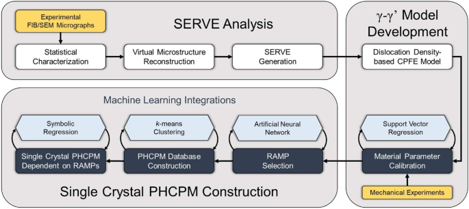

  

  Flowchart of the sequence of computational procedures in the single crystal PHCPM development process for the Ni-based superalloy René 88DT, showing integration with various machine learning techniques.

The multi-step PHCPM development process, along with the application of machine learning techniques, is depicted in Fig. 2. Machine learning is used to accelerate the computational methods in many of the steps. In the crystal plasticity model parameter calibration, optimal parameters are evaluated by a genetic algorithm (GA) with local minimization features through support vector regression. In the RAMP identification process, Sobol analysis28 and artificial neural networks20 provide the foundation for an efficient global sensitivity analysis of the $\gamma -\gamma '$ statistics. In CPFEM-generated database construction, k-means clustering offers a strategy for accelerating a large number of complex simulations during self-consistent homogenization. Symbolic regression is employed in the generation of the single crystal PHCPMs to provide functional forms for mapping RAMPs to the PHCPM constitutive parameters. The parametric homogenization process is computationally intractable without the significant efficiency enhancement afforded by these machine learning techniques.

Dislocation Density-Based Crystal Plasticity Model for $\gamma -\gamma '$ Microstructure and Parameter Calibration

The Crystal Plasticity Model

The micromechanical behavior of individual phases of the $\gamma -\gamma '$ microstructure is described by a dislocation density-based crystal plasticity constitutive model developed and detailed in Refs. 23 and 25. It captures dislocation density evolution at various temperatures, strain rates, orientations and applied loading. The finite deformation model is based on the multiplicative decomposition of the deformation gradient $\mathbf {F} = \mathbf {F}_e \mathbf {F}_p$ into a plastic component $\mathbf {F}_p$, corresponding to the mapping of reference material elements to a stress-free intermediate configuration and an elastic component $\mathbf {F}_e$. The elastic response of the material is characterized by the evolution of the second Piola-Kirchhoff stress in this intermediate configuration as:

$$\begin{aligned} \mathbf {S} = \mathbb {C}(T) : \mathbf {E}_e \end{aligned}$$

(1)

where T is temperature, $\mathbb {C}(T)$ is the temperature-dependent fourth order elasticity tensor and $\mathbf {E}_e$ is the elastic Green-Lagrange strain. For FCC and L$1_2$ structures of the $\gamma$ and $\gamma '$ phases of the superalloy exhibiting cubic symmetry, $\mathbb {C}$ reduces to three independent components. Linear temperature dependence with the same slope is assumed for all the components. Using standard Voigt notation, the components of $\mathbb {C}$ are:

$$\begin{aligned} C_{11} = C^{(0)}_{11} - \beta T, ~~C_{44} = C^{(0)}_{44} - \beta T,~~\text{ and }~~ C_{12} = C^{(0)}_{12} - \beta T \end{aligned}$$

(2)

where $\beta$ is a material constant and $C^{(0)}_{11}, C^{(0)}_{44}$ and $C^{(0)}_{12}$ are elasticity components at zero absolute temperature. The plastic flow rate of the material is kinematically confined to the crystallographic slip directions $\mathbf {m}_0^{\alpha }$ along specific slip planes $\mathbf {n}_0^{\alpha }$ for a given slip system $\alpha$. The plastic velocity gradient $\mathbf {L}_p$ is written as:

$$\begin{aligned} \mathbf {L}_p = \dot{\mathbf {F}}_p \mathbf {F}_p^{-1} = \sum _{\alpha = 1}^{N_{\mathrm{slip}}} \dot{\gamma }^{\alpha } \mathbf {m}_0^{\alpha } \otimes \mathbf {n}_0^{\alpha } \end{aligned}$$

(3)

where $N_{\mathrm{slip}}$ is the number of slip systems and $\dot{\gamma }^{\alpha }$ is the plastic slip rate. Slip occcurs on the octahedral slip systems for both the $\gamma$ and $\gamma '$ phases and additionally on cube slip systems for the $\gamma '$ precipitate phase. Following the Orowan equation, a flow rule is adopted to define the plastic slip rate as:

$$\begin{aligned} \dot{\gamma }^{\alpha } = \rho ^{\alpha }_{m} b \exp \left( -\frac{Q}{k_{B}T} \right) \text {sinh} \left( \frac{{\tau ^{\alpha }_{\mathrm{eff}}}}{\tau ^{\alpha }_{\mathrm{cut}}} \right) \text {sign}(\tau ^{\alpha }) \end{aligned}$$

(4)

where $\rho ^{\alpha }_{m}$ is the mobile dislocation density, b is the Burgers vector, Q is the activation energy for slip, and $\tau ^{\alpha }_{\mathrm{cut}}$ is the cutting stress. The effective stress is defined as $\tau ^{\alpha }_{\mathrm{eff}} := {\mathscr {H}}(|\tau ^{\alpha }| - \tau ^{\alpha }_{pass} - \tau ^{\alpha }_c)$. ${\mathscr {H}}$ is the Heaviside function, $\tau ^{\alpha } = (\mathbf {F}_e^{\text {T}} \mathbf {F}_e \mathbf {S}_p) : (\mathbf {m}_0^{\alpha } \otimes \mathbf {n}_0^{\alpha })$ is the resolved shear stress, $\tau ^{\alpha }_{pass}$ is the passing stress, and $\tau ^{\alpha }_c$ is a critical resolved shear stress. $\tau ^{\alpha }_c$ is zero for the $\gamma$ phase and is dependent on additional temperature and orientation dependent mechanisms for the $\gamma '$ phase. For a given slip system, the in-plane (parallel) and out-of-plane (forest) dislocations induce slip resistance stresses $\tau ^{\alpha }_{pass}$ and $\tau ^{\alpha }_{\mathrm{cut}}$, respectively. These slip resistance stresses are given in terms of the parallel and forest dislocation densities, $\rho ^{\alpha }_{p}$ and $\rho ^{\alpha }_{f}$, as:

$$\begin{aligned} \tau ^{\alpha }_{pass} = c_{ps} G b \sqrt{\rho ^{\alpha }_{p} + \rho ^{\alpha }_{m}}, \quad \tau ^{\alpha }_{\mathrm{cut}} = \frac{k_{B}T}{c_{av}c_{jw}b^{2}} \sqrt{\rho ^{\alpha }_{f}} \end{aligned}$$

(5)

where $c_{ps}$, $c_{av}$, $c_{jw}$ are material constants and G is the shear modulus.

The evolutions of $\rho ^{\alpha }_{p}$ and $\rho ^{\alpha }_{f}$ are formulated as projections of the overall statistically stored dislocation (SSD) density $\rho ^{\alpha }_{ssd}$ and geometrically necessary dislocation (GND) density $\rho ^{\alpha }_{gnd}$ onto the slip plane. The unstressed material contains an initial SSD density $\rho ^{\alpha }_{ssd_0}$ resulting from processing. With applied loading, this dislocation content evolves in time according to the relation:

$$\begin{aligned} \dot{\rho }_{ssd}^{\alpha } = c_{lf} \dot{\rho }_{lf}^{\alpha } + c_{df} \dot{\rho }_{df}^{\alpha } + c_{aa} \dot{\rho }_{aa}^{\alpha } + c_{ta} \dot{\rho }_{ta}^{\alpha } \end{aligned}$$

(6)

where $c_{lf}$, $c_{df}$, $c_{aa}$ and $c_{ta}$ are $\dot{\gamma }^{\alpha }$-dependent material constants controlling the competition between the dislocation multiplication and annihilation mechanisms. Further details regarding the evolution of the individual mechanisms for $\dot{\rho }_{ta}^{\alpha }$, $\dot{\rho }_{ta}^{\alpha }$, $\dot{\rho }_{ta}^{\alpha }$ and $\dot{\rho }_{ta}^{\alpha }$, as well as the evolution of $\rho _{gnd}^{\alpha }$ and $\rho _{m}^{\alpha }$, are provided in Refs. 23 and 25. The final consideration is a definition of $\tau _c^{\alpha }$ for the $\gamma '$ phase to capture anti-phase boundary (APB) shearing and cross-slip mechanisms due to KW locks. The critical resolved shear stress is given as:

$$\begin{aligned} \tau ^{\alpha }_{c} = {\left\{ \begin{array}{ll} \tau ^{\alpha }_{c,apb} + \tau ^{\alpha }_{c,kw} &{} \text {on\,octahedral\,slip\,systems} \\ \tau ^{\alpha }_{c,cube} &{} \text {on\,cube\,slip\,systems} \end{array}\right. } \end{aligned}$$

(7)

where $\tau ^{\alpha }_{c,apb} := \frac{c_{apb} \Gamma _{111}}{b}$ is the stress required for dislocations to overcome the APB energy, $\Gamma _{111}$ is the APB energy on the octahedral planes, $\tau ^{\alpha }_{c,kw}$ is the resistance due to KW locks, and $\tau ^{\alpha }_{c,cube}$ is the slip resistance stress on the cube planes. The particular non-Schmid model for $\tau ^{\alpha }_{c,kw}$, outlined in Ref. 25, is parametrized by three material properties, viz. A, $\kappa _1$ and $\kappa _2$. This slip resistance due to KW locks controls the tension-compression asymmetry, orientation dependence and temperature dependence of the material.

Summary of Experiments Used for Model Calibration

The set of experiments described in Refs. 29 and 30 for the superalloy SC-16 is chosen for calibrating the dislocation-density crystal plasticity model in Sect. 3. The composition and microstructure of SC-16 superalloy are similar to those of the René 88DT superalloy. The experiments represent a wide range of applied strain rates, load orientations and temperatures.

Eight constant strain rate experiments from29 (set ${\mathscr {E}}_1$) and six constant strain rate experiments from30 (set ${\mathscr {E}}_2$) are chosen for material parameter calibration. In the set of experiments ${\mathscr {E}}_1$, single crystals are loaded to 5% true strain, and the stress-strain plots are documented. These experiments are performed at 1123 K with all six combinations of ([001], [011], [111]) orientations and strain rates $10^{-2}s^{-1}$ and $10^{-5}s^{-1}$ and at 1223 K for the [001] orientation at both the strain rates $10^{-2}s^{-1}$ and $10^{-5}s^{-1}$. The set of experiments ${\mathscr {E}}_2$ only reports yield stresses at a constant strain rate of $10^{-3}s^{-1}$ rather than the entire stress-strain plots. The yield stresses selected for calibration from this experimental database are those derived from mechanical tests loaded to > 2.5% plastic strain. Each experiment is represented by a single combination of ([001], [011], [111]) orientations and (923 K, 1023 K) temperatures.

Genetic Algorithm-Based Calibration of Crystal Plasticity Model Parameters

The parameters in the dislocation-density crystal plasticity model for $\gamma -\gamma '$ superalloys in Sect. 3 may be grouped into four sets, expressed as:

• 1. Elasticity: $C_{11}^{(0)}$, $C_{12}^{(0)}$, $C_{44}^{(0)}$, $\beta$

• 2. Yield and Rate Sensitivity: Q, $\rho _{SSD_0}$, $c_{ps}$, $c_{jw}$, $c_{av}$, $c_{apb}$

• 3. Hardening Evolution: $c_{lf}$, $c_{df}$, $c_{aa}$, $c_{ta}$

• 4. Anomalous Yield and Tension-Compression Asymmetry: $\kappa _1$, $\kappa _2$, A

The four elastic constants in set 1 characterize the parametrization of $\mathbb {C}(T)$ in Eqs. (1) and (2). Calibrating with respect to the linear portions of the four experimental stress-strain curves corresponding to a $10^{-2}s^{-1}$ strain rate in ${\mathscr {E}}_1$ in Sect. 3.2, they are determined to be $C_{11}^{(0)} = 256$ GPa, $C_{12}^{(0)} = 185$ GPa, $C_{44}^{(0)} = 167$ GPa and $\beta = 49.2$ MPa/K.

For GA-based calibration, the 13 inelastic parameters in sets 2, 3 and 4 are lumped into a 13-dimensional material property vector, denoted as $\mathbf {P}$. The calibration process determines an optimal vector $\mathbf {P} = \mathbf {P}_*$ that matches the predictions of simulation with the experimental data set. Defining an error metric $\phi$ as the sum of simulation-experiment errors as:

$$\begin{aligned} \phi = \sum _{i\in {\mathscr {E}}_1} w_i^{(1)} \left( \frac{\int _{\epsilon } \big | \sigma _{zz}^{\text {sim}_i} - \sigma _{zz}^{\text {exp}_i} \big | \, \mathrm{d}\epsilon _{zz}}{\max \left( \sigma _{zz}^{\text {exp}_i} \right) \cdot \max \left( \epsilon _{zz}^{\text {exp}_i} \right) } \right) + \sum _{j\in {\mathscr {E}}_2} w_j^{(2)} \left( \frac{|\overline{\sigma }_{Y}^{\text {sim}_j} - \overline{\sigma }_{Y}^{\text {exp}_j} | \, \epsilon _{\mathrm{max}}}{ \overline{\sigma }_{Y}^{\text {exp}_j} \, \epsilon _{\mathrm{max}}} \right) \end{aligned}$$

(8)

$w_i^{(1)}$ and $w_j^{(2)}$ are the experiment weights with the constraint $\sum _{i\in {\mathscr {E}}_1} w_i^{(1)} + \sum _{j\in {\mathscr {E}}_2} w_j^{(2)} = 1$. The superscripts $\text {sim}_i$ and $\text {exp}_i$ denote the ith experimental and simulation variables in the set, and $\overline{\sigma }_Y$ is the yield stress as defined in Ref. 30. $\epsilon _{\mathrm{max}}$ is a fixed strain that is set to 0.05, and $\sigma _{zz}$ and $\epsilon _{zz}$ are the stress and strain components rotated into the appropriate experimental loading orientation. Determining the global minimum of $\phi$ characterizes a successful calibration, which is conducted using a machine learning-enhanced genetic algorithm (GA).

Fig. 3

Flowchart of the genetic algorithm used for material parameter calibration. The path shown by gold arrows shows the additional material parameter update provided by the support vector regression (SVR) emulation.

GAs are global optimization schemes with the ability to stochastically traverse the parameter space and avoid the pitfalls of pure gradient-based methods.31 Some of the necessary benefits of GAs for CPFE calibration include the global search to avoid local minima of $\phi$, unstructured sampling of the material property input space and massive parallelism in the implementation. The GA applied to the crystal plasticity calibration problem is outlined in Fig. 3 with the following steps:

• 1. Initialization Initialize a random set of n material parameter vectors or a “generation,” ${\mathscr {P}}^{(i)} = \{ \mathbf {P}_1^{(i)}, \mathbf {P}_2^{(i)}, \ldots , \mathbf {P}_n^{(i)} \}$.

• 2. Evaluation Evaluate the error metric $\phi$ for each choice of $\mathbf {P}_k^{(i)} \in {\mathscr {P}}^{(i)}$ to assess proximity to the experimental data.

• 3. Evolution Based on performance measured by $\phi$, determine the next generation of material properties vectors ${\mathscr {P}}^{(i+1)}$ by applying binary transformations and standard mutation/crossover operators to the previous generation ${\mathscr {P}}^{(i)}$.

• 4. Termination Repeat the process, restarting at the evaluation step with ${\mathscr {P}}^{(i+1)}$ until an optimal $\mathbf {P}_*$ is discovered in the latest generation, determined by a tolerance $\epsilon$ on $\phi$.

The evaluation step, which involves running multiple expensive micromechanical simulations, is completely parallelizable, since the error computation of each material property vector is independent of the others in the same generation.

Accelerated Calibration Error Minimization with Support Vector Regression (SVR)

A general shortcoming of GAs and other global optimization strategies is that they are prone to relatively slow convergence in comparison with gradient-based methods. To overcome this limitation, the GA is augmented by a machine learning-based approach for approximating the location of local minima. In the evolution step of the GA, mutation and crossover operators use the information of the current generation ${\mathscr {P}}^{(i)}$ to determine guesses for elements of the next generation ${\mathscr {P}}^{(i+1)}$. Instead of only pursuing parameter space guesses from these operators, an additional suggestion $\mathbf {P}_{m}^{(i+1)}$ is added to ${\mathscr {P}}^{(i+1)}$ with the goal of approximating a gradient-based estimate.

During the GA iterations, the landscape of the error metric $\phi$ is probed at an increasing number of discrete points, which is used to create a smooth representation of the landscape. The process of approximating $\phi$ falls under the regression category of supervised learning techniques. The support vector regression (SVR) method19,32 is chosen because of its ability to handle sparse data and its smoothness properties. The key feature of support vector regression is the nonlinear translation of data into an infinite-dimensional feature space, where regression is executed. The result of SVR is an emulated model of $\phi$ that does not require performing CPFE simulations to sample from it and is therefore a computationally efficient approximation of the calibration error.

For each generation of the GA, an updated SVR emulation of $\phi$ is generated through training and testing with five-fold cross-validation to the data from all previous and current generations. The material property vectors from all completed generations are assembled, normalized and replicated into five sets, each partitioned into training and testing data sets, 80% to 20%, respectively. In each of these five replicated sets, 20% different data are designated as the testing data. The SVR is trained to each of the training data sets and attempts to predict the corresponding testing data set. The accumulation of testing error over these five partitions yields the overall cross-validation error. This process is repeated for different values of SVR hyper-parameters,5,19 such as the regularization parameter and radial basis function kernel coefficient, and the cross-validation error is computed for each. The hyper-parameters, corresponding to the least cross-validation error, are selected as the SVR model parameters. Subsequently, the SVR is trained once more with all available data to generate the final emulated model of the $\phi$ landscape.

Although the actual $\phi$ is difficult to minimize, it is efficient to find local minima of its SVR emulation using the constrained Jacobian-free solver COBYLA.33,34 This procedure is followed to propose an additional candidate solution $\mathbf {P}_m^{(i+1)}$ for every new generation of GA. This feature drives the global optimization in probable directions through the material parameter space. The entire algorithm is summarized in the flowchart shown in Fig. 3.

Results of Material Parameter Calibration

For calibrating the two-phase dislocation density-based crystal plasticity model, a SERVE containing 50 precipitates is generated for the SC-16 superalloy,26,27 for which the loading conditions follow the experiments. The GA with SVR-assisted acceleration optimization strategy is applied to the 13-D material parameter space. For high dimensions, an important consideration is the method used to represent possible choices for numerical representation of material parameters. In GA, each dimension of a given $\mathbf {P}$ is a material property within some finite sampling range that is discretized into finite sampling intervals. When searching through high dimensions and many orders of magnitude, it is beneficial to transform the finite intervals of each material property into a logarithmic scale for uniform sampling across scales. The algorithm described in Fig. 3 generates the calibrated material parameters given in Table I. Comparisons between experiments and final simulation results are given in Fig. 4. Figure 4a shows the sample single crystal experimental and simulated stress-strain plots at various orientations, temperatures and strain rates that comprise a subset of the training data set ${\mathscr {E}}_1$. The validation experimental and simulated stress-strain plots for conditions [001], 1223 K, $10^{-3} \mathrm{s}^{-1}$ and [001], 1123 K, $~10^{-6} \mathrm{s}^{-1}$ are shown in Fig. 4b.

Fig. 4

(a) Calibration: sample single crystal experimental and simulated stress-strain curves at various orientations, temperatures and strain rates. (b) Validation: single crystal experimental and simulated stress-strain curves for loading cases, not part of the calibration data set.

Table I List of calibrated values of inelastic parameters

Global Sensitivity Analysis of $\gamma -\gamma '$ Microstructural Descriptors and RAMP Selection

Global Sensitivity Analysis (GSA)

The morphology of the intragranular precipitate-matrix microstructure as shown in Fig. 1 is characteristic of Ni-based superalloy single crystals. There are many possible parametrizations of these microstructures within some tolerance of their representation. Example statistical distributions that distinguish $\gamma '$ precipitate morphology include the size, aspect ratio and degree of sphericity, while characterization of $\gamma '$ precipitate spatial configurations include the two-point correlation function, local volume fraction distribution, channel-width distribution and distance-to-edge distribution.27 For parametric homogenization leading to the PHCPMs, it is prohibitive to incorporate detailed microstructural representation to the higher scale. It is important to have an optimal set of reduced parameters for representing the microstructure, while retaining the accuracy of microstructural influence on response prediction. This motivates the use of GSA to determine an optimal set of RAMPs that affect the overall yield and hardening response of the microstructural SERVE.

GSA is an uncertainty quantification method that is used to determine the degree to which each component of input $\mathbf {R}$ of a function f influences its output $\mathbf {Y}$. In the PHCPM calibration process, $\mathbf {R}$ is the vector of all candidate RAMPs considered, f is the computationally expensive crystal plasticity model, and $\mathbf {Y} := (\sigma _Y, H)$ where $\sigma _Y$ is the 0.02% offset yield stress and H is the hardening modulus defined by the best linear approximation to the slope of the stress-strain curve after reaching $\sigma _{Y}$. The candidate RAMPS included in $\mathbf {R}$ are all the parameters representing microstructural characteristics described in Ref. 27. It is a set of 19 parameters describing the statistical distributions of $\gamma '$ precipitate descriptors, e.g., radius, aspect ratio, shape, two-point correlation, distance to edge and local volume fraction.

Global sensitivity analysis, also called Sobol’ analysis or variance-based sensitivity analysis, avoids restrictive assumptions such as linearity or independence, implementation issues in high dimensions, dependence on the local behaviors of the function and unintuitive interpretations of the resultant measure.35 To overcome these issues, GSA defines multiple orders of sensitivity indices for each candidate RAMP in $\mathbf {R}$ that account for the global behavior of f.28,35 The approach is to additively decompose the variance of the mechanical response output $\mathbf {Y}$ into partial variances of conditional expected values of the components of $\mathbf {R}$. Explicitly, the variance of each mechanical output $Y^{(k)}$ in $\mathbf {Y}$ is decomposed as:

$$\begin{aligned} {\text {Var}}(Y^{(k)})= \sum ^d_{i = 1} V_i^{(k)} + \sum ^d_{i < j} V_{ij}^{(k)} + \text{higher order variance terms}, ~~~\text{ with } \end{aligned}$$

(9a)

$$\begin{aligned} V_i^{(k)}&:= {\text {Var}}_{R_i} ({\text {E}}_{{\mathbf {R}_{\sim i}}} (Y^{(k)} \, | \, R_i)) \end{aligned}$$

(9b)

$$\begin{aligned} V_{ij}^{(k)}&:= {\text {Var}}_{R_{ij}} ({\text {E}}_{{\mathbf {R}}_{\sim ij}} (Y^{(k)} \, | \, R_i, R_j)) - V_i - V_j \end{aligned}$$

(9c)

where d is the dimension of $\mathbf {R}$, $R_i$ is the ith component (candidate RAMPs) of $\mathbf {R}$, and $\mathbf {R}_{\sim i}$ is the vector containing all components of $\mathbf {R}$ except the ith component, i.e., $\mathbf {R}=\mathbf {R}_{\sim i} \cup R_i$. These definitions also apply to $V_{ij}$ for the pair of indices ij. This variance decomposition leads to the definition of the first order sensitivity index for the i-th candidate RAMP as:

$$\begin{aligned} S_i^{(k)} := \frac{V_i^{(k)}}{{\text {Var}}(Y^{(k)})} \end{aligned}$$

(10)

These sensitivity indices essentially reveal what fraction of the k-th response output variance is governed by the variance of the i-th candidate RAMP. They account for the entire input space in their computation and therefore yield a global measure of sensitivity.

To apply the sensitivity analysis framework to the micromechanical problem for Ni-based superalloys, many virtual microstructural SERVEs are created using generation methods described in Refs. 26 and 27. Each SERVE is uniaxially loaded to 5% strain and simulated using CPFEM to determine the yield and hardening response. This process is executed for about 13,000 different microstructures, characterized by different instantiations of $\mathbf {R}$. This data set creates a discrete representation of the CPFE model f that connects the microstructure parameters to the mechanical response.

Artificial Neural Network Model Emulation of Dislocation Density-Based CPFE Model

To numerically compute the sensitivity index for each candidate RAMP, the variance of the conditional expected values $\text {Var}_{R_i} ({\text {E}}_{{\mathbf {R}}_{\sim i}} (Y^{(k)} \, | \, R_i))$ is required. Thus, the conditional distribution $f(Y^{(k)} \, | \, R_i)$ must be sampled from repeatedly for many values of $R_i$. This sampling is an expensive operation since evaluating f implies performing a CPFE simulation of a SERVE. However, the computational cost is greatly reduced by using the discrete data set of generated SERVEs and the corresponding mechanical responses to create an emulated model of f for statistical sampling.

Similar to the SVR approach, a regression-type machine learning technique is trained from the discrete data to replace the expensive dislocation-density CPFE model. In this case, an artificial neural network (ANN) is selected to represent the expensive model f over SVR, since more data points exist. The ANN is trained and tested with five-fold cross-validation to the CPFE data. A three hidden layer network is selected, and the chosen hyper-parameters for cross-validation are the $L_2$ penalty regularization parameter and the number of nodes in the hidden layers. The input candidate RAMPs describing each virtual microstructure are normalized onto a unit hypercube before operations.

Selection of RAMPs for $\gamma -\gamma '$ Microstructures

The trained ANN enables rapid Monte Carlo sampling of $V_i^{(k)}$ and evaluation of the first-order sensitivity index $S_i^{(k)}$ for each candidate RAMP using Eq. 10. The sensitivity indices are used as a screening method rather than a strict variance decomposition because of complications with input covariances. The result of applying GSA to the 13,000 $\gamma -\gamma '$ microstructural SERVEs is the identification of the top-ranking sensitivity indices of RAMPs, listed in Table II.

Table II Sensitivity indices for the top six candidate RAMPs from microstructural descriptors

All the remaining candidate RAMPs in $\mathbf {R}$ yield first-order sensitivity indices < 1% and are thus excluded from the RAMP selection. In conclusion, the RAMPs considered for incorporation in the PHCPM equations are:

• ($\mu _v$, $\sigma _v$): Mean and standard deviation of the local volume fraction distribution;

• ($\mu _c$, $\sigma _c$): Mean and standard deviation of logarithm of the channel width per mean radius distribution;

• ($\mu _n$, $\sigma _n$): Mean and standard deviation of the logarithm of the shifted shape exponent distribution.

The shifted shape exponent distribution quantifies the degree of sphericity or cuboidalness of the $\gamma '$ precipitates, discussed in Ref. 27.

The mean volume fraction and mean channel width are the most dominant RAMPs with respect to the yield strength and hardening modulus. The variance of the channel width and local volume fraction also make a significant contribution to these response functions. This influence is justified by the increased dislocation flow through large $\gamma$ matrix channels devoid of $\gamma '$ precipitates, which is consistent with plastic strain localization in contour plots given in Ref. 26. The six RAMPs $\mu _v$, $\sigma _v$, $\mu _c$, $\sigma _c$, $\mu _n$ and $\sigma _n$ are representations of microstructural descriptors to be upscaled through parametric homogenization for developing the PHCPMs.

Developing the Parametrically Homogenized Crystal Plasticity Model (PHCPM) for Ni-Based Superalloy Single Crystals

Ni-based superalloys exhibit a variety of fundamental deformation characteristics such as anisotropy, strain rate and temperature dependency in their single crystal response that are attributed to deformation mechanisms in the intragranular $\gamma -\gamma '$ microstructure. The PHCPMs represent the microstructure-dependent mechanical response of the underlying complex $\gamma -\gamma '$ microstructure in an upscaled, reduced-order form. Prior to the development of PHCPMs with constitutive parameters that are explicit functions of the RAMPs, it is necessary to determine an appropriate constitutive framework, which represents the aforementioned mechanical response characteristics and is consistent with the homogenized $\gamma -\gamma '$ crystal plasticity response.12,13

Relations Defining the Single Crystal PHCPM

The chosen form of the PHCPM equations corresponds to the activation energy-based crystal plasticity model given in Ref. 36. The formulation follows from the same kinematic description in Eq. 3, but deviates from the lower-scale constitutive laws through the introduction of a thermally activated flow rule with phenomenological hardening evolution laws. With the assumption of dislocation motion being a thermally activated process, an Orowan-type flow rule defines the plastic slip rate as:

$$\begin{aligned} \dot{\gamma }^{\alpha } = \dot{\gamma }_0 \exp \left( -\frac{Q_{\mathrm{act}}}{k_B T} \left( 1 - \frac{{\mathscr {H}}(|\tau ^{\alpha }| - s_{a}^{\alpha })}{s_{*,tot}^{\alpha }} \right) \right) \text {sign} (\tau ^{\alpha }) \end{aligned}$$

(11)

where $\dot{\gamma }_0$ is the reference slip rate, $Q_{\mathrm{act}}$ is the activation energy for slip, $k_B$ is the Boltzmann constant, and $\tau ^{\alpha }$ is the resolved shear stress. The athermal slip resistance $s_a^{\alpha }$ is due to parallel dislocations, and $s_{*,tot}^{\alpha } := s_{*}^{\alpha } + s_{cross}^{\alpha }$ is composed of the thermal slip resistance due to forest dislocations $s_{*}^{\alpha }$ and an additional cross slip resistance $s_{cross}^{\alpha }$ due to the temperature-dependent formation of Kear-Wilsdorf locks.

Self-hardening and latent hardening effects are dependent on the in-plane and out-of-plane multiplication and flow of dislocations. Initial values are prescribed for both athermal and thermal slip resistances, $s_{a0}$ and $s_{*0}$. The evolution of these slip resistances is governed by:

$$\begin{aligned} \begin{aligned} \dot{s}_a^{\alpha }&= \sum ^{N_{\mathrm{slip}}}_{\beta = 1} h_a^{\alpha \beta } |\dot{\gamma }^{\beta } \sin (\mathbf {n}_0^{\beta }, \mathbf {t}_0^{\beta })| \\ \dot{s}_*^{\alpha }&= \sum ^{N_{\mathrm{slip}}}_{\beta = 1} h_*^{\alpha \beta } |\dot{\gamma }^{\beta } \cos (\mathbf {n}_0^{\beta }, \mathbf {t}_0^{\beta })| \\ \end{aligned} \end{aligned}$$

(12)

where $\mathbf {t}_0^{\alpha } := \mathbf {m}_0^{\alpha } \times \mathbf {n}_0^{\alpha }$, and $h_a^{\alpha \beta }$ and $h_*^{\alpha \beta }$ are matrices of interaction coefficients between slip systems. For simplicity, the interaction coefficients are assumed to be equivalent, i.e., $h^{\alpha \beta }$ = $h_a^{\alpha \beta }$ = $h_*^{\alpha \beta }$. They evolve and saturate according to:

$$\begin{aligned} h^{\alpha \beta } = q^{\alpha \beta } h^{\beta } \quad \text {where} \quad h^{\beta } = h_0 \Bigg | 1 - \frac{s^{\beta }}{s^{\beta }_{sat}} \Bigg |^{r} \text {sign} \left( 1 - \frac{s^{\beta }}{s^{\beta }_{sat}} \right) \end{aligned}$$

(13)

where $s^{\beta }_{sat}$ is the saturation slip resistance, r is the saturation rate exponent, $q^{\alpha \beta }$ are hardening coefficients, and $h_0$ is the initial hardening parameter. Values of the material parameters and details of this constitutive law are given in Ref. 36.

Two constitutive parameters that govern the yield and hardening behavior are selected as RAMP-dependent variables for establishing a direct connection to the underlying complex $\gamma -\gamma '$ microstructure. These are the initial thermal slip resistance $s_{*0}$ and the initial hardening parameter $h_0$. Let the vector of these material parameters be denoted $\mathbf {M} := (s_{*0} \, , h_0)$. Determining the explicit mapping from the RAMPs to the material parameter vector $\mathbf {M}$ of the PHCPM is a primary goal.

Self-consistent Homogenization for Determining Upscaled Response

Homogenization or volume-averaging of the SERVE response for developing the PHCPMs requires the solution of the SERVE-based micromechanical problem with appropriate boundary conditions. Various approaches have been suggested to define boundary conditions for heterogeneous micromechanical models for homogenization. They include the periodic boundary conditions,37 affine boundary conditions and self-consistent schemes.37,38,39 The self-consistent methodology, as shown in Fig. 5a, is selected for constructing the PHCPMs in this work. The multiscale domain consists of an intragranular $\gamma -\gamma '$ SERVE that is embedded in an outer homogeneous domain defined by the PHCPM constitutive behavior. The interface is constructed as a handshake region with overlapping homogeneous and heterogeneous domains. Displacement continuity is enforced on both boundaries of the handshake region, and traction continuity is satisfied on the heterogeneous-handshake interface. A self-consistency condition is enforced within the handshake domain, which is the solution to the problem defined as:

$$\begin{aligned}&\text{Find\,the\,set\,of\,homogenized\,material\,parameters}\,\mathbf {M}_*\,{\text {such\,that:}} \nonumber \\&\mathbf {M}_* = \underset{\mathbf {M}}{\text {arg\,min}} \left( \Psi \right)\,\text {with} \end{aligned}$$

(14a)

$$\begin{aligned}&\Psi = \int _0^t \Big | \int _{\Omega } {\varvec{\Sigma }} (\mathbf {M}) : \mathbf {D}(\mathbf {M}) \, \text {d} \Omega - \int _{\Omega } {\varvec{\sigma }} : \mathbf {d} \, \text {d} \Omega \Big | \, \text {d} t \end{aligned}$$

(14b)

where ${\varvec{\Sigma }} (\mathbf {M})$ is the Cauchy stress and $\mathbf {D}(\mathbf {M})$ is the rate of deformation tensor in the PHCPM-based homogeneous domain, while ${\varvec{\sigma }}$ is the Cauchy stress and $\mathbf {d}$ is the rate of deformation tensor in the heterogeneous $\gamma -\gamma '$ domain.

Fig. 5

(a) Multiscale domain for self-consistent homogenization, consisting of an intragranular $\gamma -\gamma '$ SERVE embedded in a PHCPM-defined homogeneous domain with a handshake interface region for satisfying self-consistency conditions, and (b) comparing the elastic and plastic energy densities as a function of the true strain in the PHCPM-based homogeneous and CPFEM-based heterogeneous regions of the multiscale domain, after convergence of the self-consistent $\mathbf {M}_*$. The results are for a uniaxial [001] constant strain rate loading.

The self-consistency condition of Eq. 14a defines an optimization problem. For a fixed heterogeneous SERVE with a fixed set of RAMPs, multiple coupled simulations must be performed in an iterative procedure to determine the optimal $\mathbf {M}_*$. This set of iterations is very computationally expensive and is a major factor in limiting the parametric homogenization process. A procedure is first described to demonstrate a base strategy to execute this material property optimization. Subsequently, it is shown in Sect. 5.3 that employing a modification invoking an unsupervised learning technique, viz. k-means clustering,21 greatly improves the efficiency of the procedure and makes the optimization computationally feasible.

For a given embedded heterogeneous microstructure and a chosen external loading, the base optimization process solves for (i) the deformation history $\mathbf {F}(\mathbf {X}, t)$ of every material point $\mathbf {X}$ through time t and (ii) simultaneously for the self-consistent, optimal $\mathbf {M}_*$ in a staggered iterative fashion. Major steps of the procedure are delineated as:

• 1. Initialize With an initial guess $\mathbf {M}^{(i)}$ for material properties of the homogeneous region, the multiscale domain with the embedded SERVE in Fig. 5a is simulated for a given load history on the external boundary. The simulation yields a time-evolving displacement field for every node of the mesh and consequently the time-dependent deformation gradient $\mathbf {F}^{(i)}$ at every integration point of the element. The initial estimates of $\mathbf {M}^{(i)}$ are unlikely to satisfy self-consistency and need iterative update.

• 2. Holding $\mathbf {F}^{(i)}$ fixed, find $\mathbf {M}^{(i+1)}$ Next, the deformation history for every element is held fixed at the values obtained from step 1 and applied respectively to each element of the homogeneous mesh separately. This decouples the stress response and state variables in each element from those of its contiguous neighbors. A new generation of $\mathbf {M}^{(i+1)}$ is created by optimizing for the material property vector that best satisfies the self-consistency expression in Eq. 14a for the decoupled problem. This decoupling facilitates the search for the next $\mathbf {M}^{(i+1)}$ satisfying the self-consistency condition. However, it does not account for global equilibrium and the element boundary displacement, which are both restored through corrective iteration.

• 3. Holding $\mathbf {M}^{(i+1)}$ fixed, find $\mathbf {F}^{(i+1)}$ With the new generation of $\mathbf {M}^{(i+1)}$, the multiscale domain is loaded again to find a new set of deformation histories $\mathbf {F}^{(i+1)}$ for each element. The staggered, iterative algorithm in steps 2 and 3 is continued until convergence of $\mathbf {M}^{(i+1)}$ is reached.

Accelerated Strategy for Parametric Homogenization with k-Means Clustering of Deformation Histories

Determining the self-consistent $\mathbf {M}_*$ is a computationally expensive undertaking. It is necessary to accelerate the optimization performed in Step 2 of Sect. 5.2, i.e., searching for the next self-consistent $\mathbf {M}^{(i+1)}$ for each fixed set of decoupled deformation histories $\mathbf {F}^{(i)}$. An unsupervised learning technique viz. k-means clustering21 is applied for this acceleration. The essential idea is to recognize that self-consistency is a volume-averaged measure and can be approximately satisfied by performing an optimization on a reduced number of representative elements undergoing characteristic decoupled deformation histories.

The k-means clustering algorithm attempts to group similar mathematical objects into k groups by minimizing variance in intra-group distance. Applying k-means to the optimization problem provides an appropriate method to choose representative elements and their respective weightings. Accordingly, the unsupervised clustering of deformation histories requires the definition of an inner product to quantify the degree of closeness between time-dependent deformation histories of any two elements. The selected inner product ${\mathscr {I}}$ of the deformation history of $\mathbf {X}_i$ and that of $\mathbf {X}_j$ is given as:

$$\begin{aligned} {\mathscr {I}}(\mathbf {F}_{\mathbf {X}_i}, \mathbf {F}_{\mathbf {X}_j}) = \frac{\int _0^T ( \mathbf {F}(\mathbf {X}_i, t) - \mathbf {F}(\mathbf {X}_j, t)) : (\mathbf {F}(\mathbf {X}_i, t) - \mathbf {F}(\mathbf {X}_j, t)) \, \mathrm{d}t}{\int _0^T \, \mathrm{d}t} \end{aligned}$$

(15)

where T is the total time of the simulation and $\mathbf {F}_{\mathbf {X}}(t) := \mathbf {F}(\mathbf {X}, t)$. The k-means algorithm searches for a set of k representative groups ${\mathscr {F}} = \{ {\mathscr {F}}_1, {\mathscr {F}}_2, \ldots , {\mathscr {F}}_k \}$, where each group is the deformation history for a set of elements. The optimal partition of k groups is defined as:

$$\begin{aligned} {\mathscr {F}}_* = \underset{{\mathscr {F}}}{\text {arg\,min}} \sum _{p = 1}^k \left( \sum _{{\varvec{\mathbf {F}_{\mathbf {X}} \in {\mathscr {F}}_q}}} {\mathscr {I}}(\mathbf {F}_{\mathbf {X}}, \hat{\mathbf {F}}_{\mathbf {X}}^q) \right) \end{aligned}$$

(16)

where $\hat{\mathbf {F}}_{\mathbf {X}}^q$ is the mean or representative deformation history for the q-th group of deformation histories ${\mathscr {F}}_q$. Each cluster is therefore represented by a mean deformation history. In the limit, $k=1$ approximately corresponds to volume-averaging the deformation histories of all elements and applying it to a single element, while $k = N_{\mathrm{elements}}$ corresponds to simulating every element with its respective decoupled deformation history. A sufficient number of clusters is determined to be about 100-200 by assessing the incremental error reduction with the addition of new clusters.

Within step 2, for each fixed set of deformation history $\mathbf {F}^{(i)}$, clusters are established and integration points are simulated under their representative decoupled deformation histories for successive iterations of $\mathbf {M}^{(i+1)}$. The sequence of choices for $\mathbf {M}^{(i+1)}$ is the outcome of the numerical optimizer, where the objective function is the self-consistency condition. For this approximation, the integral in the self-consistency Eq. 14a is modified to be the weighted volume average of the mechanical response. The weight of each representative deformation history is the total volume of all the elements associated with the group.

The staggered iterative algorithm typically requires only 2-3 iterations of trial deformation histories to find a self-consistent $\mathbf {M}_*$ with < 1% error. A representative plot of the satisfaction of the self-consistency condition is shown in Fig. 5b for a constant strain rate loading of the multiscale domain. The volume-averaged elastic and plastic energy densities are defined as ${\varvec{\sigma }} : \mathbf {d}_e$ and ${\varvec{\sigma }} : \mathbf {d}_p$, respectively, where $\mathbf {d}_e$ and $\mathbf {d}_p$ are the elastic and plastic rate of deformation tensors in the deformed configuration. These are compared to demonstrate the efficacy of the homogenization procedure. This method provides a tremendous speedup to an otherwise numerically intractable optimization problem. The self-consistent homogenization procedure is next applied to about 120 microstructural SERVEs, characterized by different instantiations of RAMPs, for different loading orientations. For each SERVE, the procedure associates a particular set of RAMPs to a computed $\mathbf {M}_*$. These linkages between microstructure and material properties are stored in a database and are the basis for the final stage of parametric homogenization.

Microstructure RAMPs to Material Property Mappings for Single Crystal PHCPM

Symbolic Regression for RAMPs to Material Property Mapping

This is the final step in the PHCPM development. It creates an explicit mapping between the RAMPs characterizing the intragranular $\gamma -\gamma '$ microstructure and the material properties of the homogeneous single crystal plasticity constitutive model. The database generated in the previous section is a discrete representation of this mapping. Supervised learning tools are used in this section to provide functional forms of the PHCPM constitutive parameters in terms of RAMPs. The symbolic regression method22,40 is selected for its efficacy, ability to provide quick intuitions into the trends of the database and differentiability properties, which enable further analysis techniques such as uncertainty propagation.15

The symbolic regression method searches for a functional representation between inputs and outputs. It generates nested functions as a graph of elementary function evaluations, such as $\sin x$ and $x^2$, connected by common operations, such as addition and multiplication. The goal of the optimization process is to search over the space of all graphs of this type to identify the particular one that best represents the input-output relationship of the database. Genetic programming is used to explore the space of candidate graphs for symbolic regression. It is a global optimization method similar to GA. A generation of candidate graphs is proposed and evaluated on its performance at learning an input-output data set. A new generation is evolved from the current generation by applying mutation and crossover operators. The operators essentially flip nodes and swap subtrees between the best graphs of the generation. The evolutionary algorithm is repeated until the best functional representation of the data is discovered within an error tolerance. Further details of supplementing this process to penalize complexity and enable cross-validation methods are provided in Ref. 41.

The symbolic regression method operates on the database generated from self-consistent homogenization of the $\gamma -\gamma '$ SERVEs. The first $90\%$ of the generated SERVEs and their corresponding homogenized values of $\mathbf {M}$ are used to determine and calibrate the symbolic regression model. The remaining $10\%$ of the database is retained as data for model validation. The specific symbolic regression software package HeuristicsLab42 is used in this study. The resulting functional expression of each component of $\mathbf {M}$ as a function of the RAMPs is given below. These are the fundamental components of the PHCPM.

Results of Simulations with the Single Crystal PHCPM

The performance of the resulting PHCPM in Eqs. 11–13 with symbolic regression trained functional expressions in Eqs. 17 and 18 is assessed in this section. Figure 6 shows a comparison of the constitutive parameters $s_{*0}$ and $h_0$ generated from expressions (17) and (18) with given values of RAMPs, with the actual calibration data that evolves from self-consistent homogenization. Different RAMP values in this comparison correspond to different realizations of the SERVE in the multiscale domain of the self-consistent homogenization process. Ninety percent of the homogenized constitutive parameter database from all SERVEs is used for the calibration of the coefficients of Eqs. (17) and (18), while 10% is retained for validation. The validation results show that for both $s_{*0}$ and $h_0$, the predicted values are generally within an acceptable error tolerance error, implying satisfactory accuracy.

Fig. 6

Comparing constitutive parameters (a) $s_{*0}$ and (b) $h_0$ generated from expressions (17) and (18) with given values of RAMPs, with the actual data that evolves from self-consistent homogenization.

A significant advantage of the PHCPM-based FE simulations is that they provide tremendous computational efficiency in comparison with detailed micromechanical CPFEM simulations. Two examples are conducted to illustrate the speedup from PHCPM-based simulations, and the results are provided in Table III. The results correspond to a total strain of 5%. The first example compares the CPU time of detailed CPFEM simulations of a $\gamma -\gamma '$ SERVE containing 50 $\gamma '$ precipitate with that for a single integration point of PHCPM-based FE simulations. The PHCPM-based simulations show speedup by a factor of $\approx 10^6$ in the computational time. In the second example, a single grain in a polycrystalline superalloy of average grain size $\approx 15.2~\mu \text {m}$ is modeled. The single crystal FE mesh consists of 2500 linear tetrahedral elements. The underlying $\gamma -\gamma '$ microstructure has an average precipitate size of $65~\text {nm}$. A single crystal of volume $1.47 \times 10^{13} ~\text {nm}^3$ can accommodate between 1 and 10 million precipitates at a volume fraction of $\sim 30\%$. The corresponding simulation times are given in Table III.

Table III Comparison of simulation time per CPU core for various simulation domains, demonstrating the tremendous computational efficiency of the PHCPM

Conclusion

The objective of this article is to establish a comprehensive multiscale modeling framework for developing the parametrically homogenized crystal plasticity model (PHCPM) for single crystal Ni-based superalloys. Single crystals of these materials are characterized by an underlying $\gamma -\gamma '$ microstructure with a dispersion of $\gamma '$ precipitates. The PHCPMs explicitly incorporate the relevant statistics of lower scale $\gamma -\gamma '$ descriptors in the single crystal plasticity relations. This enables highly efficient and accurate image-based polycrystalline microstructural simulations without the need for exorbitant simulations of complex $\gamma -\gamma '$ microstructures. An additional advantage of the PHCPMs is that they can be readily used for representing spatial variations in the $\gamma -\gamma '$ morphology in the polycrystalline microstructures.

The single crystal PHCPM development process involves a sequence of computational methods, with explicit use of machine learning. These include: (1) construction of SERVEs for intragranular $\gamma -\gamma '$ microstructures of single crystals, (2) image-based simulations of SERVEs with experimentally calibrated dislocation-density crystal plasticity models, (3) identification of representative aggregated microstructural parameters (RAMPs) for the $\gamma -\gamma '$ microstructure-response mapping, (4) selection of a PHCPM constitutive framework and (5) performing self-consistent homogenization using a multiscale domain to establish functional expressions of PHCPM constitutive coefficients in terms of RAMPs.

Novel integration of machine learning tools is explored at every development phase for establishing relations, while overcoming major computational bottlenecks. For constitutive parameter calibration of the CPFE model, rapid minimization of calibration error in a high-dimensional input space is enabled by the use of SVR model emulation in a genetic algorithm (GA) framework. Various stochastic and heuristic global optimization techniques, such as the ant colony optimization and particle swarm optimization, are suitable for this application. However, the key features of GAs that make them desirable for this calibration are: (1) the ability to randomly sample any point in the input space with some probability in an unstructured manner, (2) the ability to favor sampling local regions of the input space near probable locations of minima, (3) massive parallelism within each generation and (4) quick computations to move to the next generation. These characteristics enable the SVR enhancement to create and explore refined locally convex regions while retaining a global depiction of the objective function landscape.

For global sensitivity analysis-based identification of RAMPs, an artificial neural network provides a means of sampling high-dimensional conditional distributions constructed from relatively scarce and expensive data. For self-consistent homogenization, k-means minimizes the PHCPM material parameter search optimization to only a few iterations of reduced order computations. For generating the RAMP to PHCPM constitutive coefficient mapping, symbolic regression yields a simple and accurate representation of the relationship that bridges the material behavior across length scales. The combination of these unique machine learning tools with a structured approach to multiscale modeling enables rigorous upscaling for image-based microstructural modeling.

The single crystal PHCPM exhibits orders of magnitude speedup over its explicit microstructure counterpart. This capability permits location-specific analysis of $\gamma -\gamma '$ intragranular microstructures within polycrystalline ensembles. In summary, the PHCPM development process demonstrates the seamless integration of physics-based models and data-driven methods to create significantly computationally advantageous models for material response in the ICME paradigm.

References

Committee on Integrated Computational Materials Engineering Pollock, T. Integrated Computational Materials Engineering: A Transformational Discipline for Improved Competitiveness and National Security. National Academies Press Washington, DC (2008)
S Ghosh, C Przybyla, C Woodward (2020) Integrated Computational Materials Engineering (ICME): Advancing Computational and Experimental Methods. Springer, Berlin
Committee on Frontiers of Materials Research Greene, L. Frontiers of Materials Research: A Decadal Survey. National Academies Press, Washington, DC (2019)
J.A Warren. MRS Bull. 43(6), 452 (2018)
F. Pedregosa, G. Varoquaux, A. Gramfort, V. Michel, B. Thirion, O. Grisel, M. Blondel, P. Prettenhofer, R. Weiss, and V. Dubourg. J. Mach. Learn. Res. 12, 2825–2830 (2011)
M. Abadi, P. Barham, J. Chen, Z. Chen, A. Davis, J. Dean, M. Devin, S. Ghemawat, G. Irving, and M. Isard, Tensorflow: A system for large-scale machine learning. in 12th USENIX Symposium on Operating Systems Design and Implementation (OSDI 16) (2016), pp. 265–283
G. Bradski, The OpenCV Library. Dr. Dobb’s Journal of Software Tools (2000)
B.L. Boyce and M.D. Uchic. MRS Bull. 44(4), 273–280 (2019)
Y. Adachi, N. Sato, M. Ojima, M. Nakayama, and Y.T. Wang, Development of fully automated serial-sectioning 3d microscope and topological approach to pearlite and dual-phase microstructure in steels. in Proceedings of the 1st International Conference on 3D Materials Science (Springer, 2012), pp. 37–42
M.P. Echlin, A. Mottura, C.J. Torbet, and T.M. Pollock, Rev. Sci. Instrum. 83(2), 023701 (2012)
M.L. Green, C.L. Choi, J.R. Hattrick-Simpers, A.M. Joshi, I. Takeuchi, S.C. Barron, E. Campo, T. Chiang, S. Empedocles, J.M. Gregoire, et al., Appl. Phys. Rev. 4(1), 011105 (2017)
S. Kotha, D. Ozturk, and S. Ghosh, Int. J. Plast. 120, 296–319 (2019)
S. Kotha, D. Ozturk, and S. Ghosh, Int. J. Plast. 120, 320–339 (2019)
D. Ozturk, S. Kotha, A. L. Pilchak, and S. Ghosh, J. Mech. Phys. Sol. 128, 181–207 (2019)
D. Ozturk, S. Kotha, A.L. Pilchak, and S. Ghosh, JOM 71(8), 2657–2670 (2019)
R.W. Kozar, A. Suzuki, W.W. Milligan, J.J. Schirra, M.F. Savage, and T.M. Pollock, Mater. Trans. A 40(7), 1588–1603 (2009)
P.A.S. Reed, Mater. Sci. Tech. 25(2), 258–270 (2009)
A. Cruzado, J. Lorca, and J. Segurado, Int. J. Solids Struct. 122, 148–161 (2017)
A.J. Smola, Stat. Comp. 14(3), 199–222 (2004)
M.H. Hassoun. Fundamentals of Artificial Neural Networks. MIT Press, Cambridge, MA (1995)
J.A. Hartigan and M.A. Wong, J. R. Stat. Soc. 28(1), 100–108 (1979)
G. Kronberger, S. Wagner, M. Kommenda, A. Beham, A. Scheibenpflug, and M. Affenzeller, Knowledge discovery through symbolic regression with heuristiclab. in Joint European Conference Machine Learning and Knowledge Discovery in Databases, (Springer, 2012), pp. 824–827
S. Keshavarz and S. Ghosh, Acta Mater. 61(17), 6549–6561 (2013)
S. Ghosh, G. Weber, and S. Keshavarz, Mech. Res. Commun. 78, 34–46 (2016)
S. Keshavarz, S. Ghosh, A. Reid, and S.A. Langer, Acta Mater. 114, 106–115 (2016)
M. Pinz, G. Weber, W.C. Lenthe, M.D. Uchic, T.M. Pollock, and S. Ghosh, Acta Mater. 157, 245–258 (2018)
M. Pinz, G. Weber, and S. Ghosh, Comput. Mater. Sci. 167, 198–214 (2019)
I.M. Sobol’, Matematicheskoe modelirovanie 2(1), 112–118 (1990)
B. Fedelich, Int. J. Plast. 18(1), 1–49 (2002)
W. Österle, D. Bettge, B. Fedelich, and H. Klingelhöffer, Acta Mater. 48(3), 689–700 (2000)
D. Whitley, Stat. Comp. 4(2), 65–85 (1994)
C.-C. Chang and C.-J. Lin, ACM Trans. Intell. Syst. Tech. (TIST) 2(3), 1–27 (2011)
M.J.D. Powell, A direct search optimization method that models the objective and constraint functions by linear interpolation. in Advances in Optimization and Numerical Analysis, (Springer, 1994), pp. 51–67
P. Virtanen, R. Gommers, T.E. Oliphant, M. Haberland, T. Reddy, D. Cournapeau, E. Burovski, P. Peterson, W. Weckesser, J. Bright, S.J. van der Walt, M. Brett, J. Wilson, K.J. Millman, N. Mayorov, A.R.J. Nelson, E. Jones, R. Kern, E. Larson, C.J. Carey, I. Polat, Y. Feng, E.W. Moore, J.V. erPlas, D. Laxalde, J. Perktold, R. Cimrman, I. Henriksen, E.A. Quintero, C.R Harris, A.M. Archibald, A.H. Ribeiro, F. Pedregosa, and P. van Mulbregt, SciPy 1. 0 Contributors, Nat. Methods 17, 261–272 (2020)
A. Saltelli, Global sensitivity analysis: an introduction. in Proceedings of 4th International Conference on Sensitivity Analysis of Model Output (SAMO’04), (Citeseer, 2004), pp. 27–43
A. Bagri, G. Weber, J.-C. Stinville, W. Lenthe, T. Pollock, C. Woodward, and S. Ghosh, Metal. Mater. Trans. A 49(11), 5727–5744 (2018)
S. Ghosh, D.V. Kubair, J. Mech. Phys. Solids 95, 1–24 (2016)
S. Nemat-Nasser, Mech. Mater. 31(8), 493–523 (1999)
S. Ghosh, J. Bai, and P. Raghavan, Mech. Mater. 39(3), 241–266 (2007)
G.F. Smits and M. Kotanchek. Pareto-front exploitation in symbolic regression. in Genetic Programming Theory and Practice II, (Springer, 2005), pp. 283–299
G. Kronberger, M. Kommenda, and M. Affenzeller, Overfitting detection and adaptive covariant parsimony pressure for symbolic regression. in Proceedings of 13th Annual Conference on Companion on Genetic and Evolutionary Computation, pp. 631–638 (2011)
S. Wagner, G. Kronberger, A. Beham, M. Kommenda, A. Scheibenpflug, E. Pitzer, S. Vonolfen, M. Kofler, S. Winkler, V. Dorfer, et al., Architecture and design of the heuristiclab optimization environment. in Advanced Methods and Applications in Computational Intelligence, (Springer, 2014), pp. 197–261
Acknowledgements
This research has been supported by a grant from the National Science Foundation, Mechanics of Materials and Structures (MOMS) Program through grant no. CMMI-1825115 (Program Manager: Dr. Siddiq Qidwai). The authors gratefully acknowledge this support. Computing support by the Homewood High Performance Compute Cluster (HHPC) and Maryland Advanced Research Computing Center (MARCC) is gratefully acknowledged.
Author information
Authors and Affiliations
Corresponding author
Ethics declarations
Conflict of interest
On behalf of all authors, the corresponding author states that there is no conflict of interest.
Additional information
Publisher's Note
Springer Nature remains neutral with regard to jurisdictional claims in published maps and institutional affiliations.
Rights and permissions
About this article
Cite this article
Weber, G., Pinz, M. & Ghosh, S. Machine Learning-Aided Parametrically Homogenized Crystal Plasticity Model (PHCPM) for Single Crystal Ni-Based Superalloys. JOM 72, 4404–4419 (2020). https://doi.org/10.1007/s11837-020-04344-9
Received:
Accepted:
Published:
Issue Date:
DOI: https://doi.org/10.1007/s11837-020-04344-9