The Influence of Horizontal Variability of Hydraulic Conductivity on Slope Stability under Heavy Rainfall

Abstract

Due to the natural variability of the soil, hydraulic conductivity has significant spatial variability. In the paper, the variability of the hydraulic conductivity is described by assuming that it follows a lognormal distribution. Based on the improved Green–Ampt (GA) model of rainwater infiltration, the analytical expressions of rainwater infiltration into soil with depth and time under heavy rainfall conditions is obtained. The theoretical derivation of rainfall infiltration is verified by numerical simulation, and is used to quantitatively analyze the effect of horizontal variability of the hydraulic conductivity on slope stability. The results show that the variability of the hydraulic conductivity has a significant impact on rainwater infiltration and slope stability. The smaller the coefficient of variation, the more concentrated is the rainwater infiltration at the beginning of rainfall. Accordingly, the wetting front is more obvious, and the safety factor is smaller. At the same time, the higher coefficient of variation has a negative impact on the cumulative infiltration of rainwater. The larger the coefficient of variation, the lower the cumulative rainwater infiltration. The conclusions reveal the influence of the horizontal variation of hydraulic conductivity on rainwater infiltration, and then the influence on slope stability.

1. Introduction

Hydraulic conductivity is an important factor affecting rainwater infiltration, and then inducing landslides. Rainwater infiltration into soil causes the increase in soil’s saturation and the corresponding decrease in matrix suction. On the other hand, rainwater infiltration also will lead to an increase in soil weight. All these adversely affect slope stability [1]. Due to the differences in material composition, settlement conditions, stress history, and geological effects, etc., slope soil has significant spatial variability of hydraulic conductivity [2,3,4]. In fact, among all the soil parameters, the hydraulic conductivity shows the strongest variability, and the resulting impact on rainwater infiltration has to be considered in the slope stability analysis. The coefficient of variation (CoV) of some soil parameters is shown in

Table 1. Variation coefficient of different soil parameters.

Property	Soil Classification	CoV (%)	Source
Unit weight (γ)		3–7	[5]
Natural water content (wn)	Clay and silt	8–30
Liquid limit (wL)	Clay and silt	6–30	[6]
Plasticity index (PI)	Clay and silt	10–40
Effective stress friction angle (°)		2–13	[7]
Undrained shear strength (su) 1	Clay	10–40
Undrained shear strength (su) 2	Clay	7–25	[6]
	Saturated clay	68–90	[5]
Hydraulic conductivity	Partly saturated clay	130–240	[8]
	-	200–300	[9]

¹ Unconfined compression test; ² Unconsolidated-undrained triaxial compression test.

.

Table 1 shows that the degree of variation of the saturated hydraulic conductivity is the strongest. Therefore, scholars around the world have extensively discussed the influence of the variability of the hydraulic conductivity on infiltration, and the impact on slope stability. Santoso et al. [10] regarded the saturated hydraulic conductivity as the random field of the static lognormal distribution, discussed the influence of the spatial variability of the saturated hydraulic conductivity along the depth direction on the infiltration of unsaturated soil by using the subset simulation method, and proposed probabilistic framework for evaluating unsaturated slope stability. Jiang et al. [11] proposed a non-intrusive stochastic finite element method for stability analysis of unsaturated soil slopes based on Latin hypercube sampling, considering the spatial variability of multiple soil parameters, and carried out reliability analysis of unsaturated soil slopes under steady seepage conditions.

The Monte Carlo method is often used in random field simulation. Based on the Monte Carlo method, Qin et al. [12] established a model for bedrock layer slope stability considering the variation of hydraulic conductivity, and analyzed the effect of the variation coefficient of hydraulic conductivity and rainfall intensity on the failure probability of landslides. Zhu et al. [3] used the fast Fourier transform technique to generate the random field of saturated permeability coefficient, and then studied the influence of the variation of the hydraulic conductivity on the slope stability under rainfall conditions based on the Monte Carlo method. Zhang et al. [13] proposed a probabilistic method for predicting the occurrence time of rainfall-induced landslides considering the variability of hydraulic conductivity based on the physical infiltration model and the Monte Carlo method. Dou et al. [14] regarded the saturated permeability coefficient as a non-stationary random field, and considered the decreasing trend of soil hydraulic conductivity with depth. Based on the Monte Carlo method the one-dimensional non-stationary random field model was established.

Cho [15] developed a one-dimensional random field model based on KL (Karhunen–Loeve) to establish the spatial variability of saturated permeability coefficient, and discussed the failure mechanism of shallow weathered residual soil slope under rainfall conditions. Li et al. [16] constructed a geological disaster meteorological risk early warning model based on the information method, and took a certain area of Honghe Prefecture as an example to provide early warning of geological disasters such as rainfall-induced landslides. Zhu et al. [17] undertook stochastic infinite slope analysis by assuming saturated hydraulic conductivity as the only random variable to assess the effect of depth on slope stability. The spatial variability of the saturated hydraulic conductivity considering the depth dependency is generated using the generic random field theory. The results show that if the depth dependency is not considered, the probability of failure is incorrectly estimated.

The above studies are almost based on the numerical simulation of the random field with hydraulic conductivity. In general, the Monte Carlo method is used to generate the random field of hydraulic conductivity. Then, slope stability analysis is carried out for these random fields, and the failure probability of the slope is obtained. All these methods require a large number of random fields to be simulated. On the one hand, the calculation efficiency is low. Secondly, we can only qualitatively study the effect of the horizontal variability of hydraulic conductivity on slope stability.

In this paper, we focus on the quantitative analysis of the influence of horizontal variability of hydraulic conductivity on slope stability. The structure of the paper is as follows. First, hydraulic conductivity is considered as a random variable, and a random variable model is used to describe the variability of hydraulic conductivity. Second, based on the improved Green–Ampt (GA) model of rainwater infiltration, the analytical solution of rainwater infiltration with depth and time under heavy rainfall conditions are obtained. Third, the safety factors of infinite slope under heavy rainfall conditions are calculated based on the theory of unsaturated soil strength. In the end, the quantitative analysis of the effect of the horizontal variability of hydraulic conductivity on slope stability is implemented.

2. Variability of Hydraulic Conductivity

The variability of hydraulic conductivity is due to its heterogeneity in spatial distribution, and is affected by many factors. Field experiments conducted by Lei et al. [18] showed that the ratio of the maximum value to the minimum value of soil hydraulic conductivity measured on a 40 m × 70 m plot could reach 1426, showing significant horizontal variability of hydraulic conductivity. In addition, when the rainfall period is short and the intensity is high, rainfall-induced landslides are generally shallow landslides, and the landslide body is generally longer. In this case, the influence of the variability on rainwater infiltration cannot be ignored. Therefore, in slope design or landslide prediction, when hydraulic conductivity is taken as a constant value without considering its variability, rainwater infiltration into the landslide body will not be correctly reflected, and the impact of rainwater infiltration on the slope stability also cannot be correctly evaluated. Many people have studied the variability of hydraulic conductivity. In general, the saturated hydraulic conductivity $K_s$ is considered to follow a lognormal distribution, and the mean ${\mu }_{K_s}$, variance ${\sigma }_{K_s}$ or CoV of the saturated hydraulic conductivity are used to describe its probability distribution. Correspondingly, $\ln K_s$ is a random variable that obeys a normal distribution, ${\mu }_{\ln K_s}$ and ${\sigma }_{\ln K_s}$ are its mean and variance respectively. The relationship between the parameters is expressed as follows:

$${\sigma }_{\ln K_s}^2=\ln \left(1+\frac{{\sigma }_{K_s}^2}{{\mu }_{K_s}^2}\right)=\ln \left(1+Co{V}^2\right),$$

(1)

$${\mu }_{\ln K_s}=\ln \left({\mu }_{K_s}\right)-\frac{1}{2}{\sigma }_{\ln K_s}^2,$$

(2)

The probability density function of saturated hydraulic conductivity $K_{\mathrm{s}}$ is expressed as:

$$f\left(K_{\mathrm{s}}\right)=\frac{1}{\sqrt{2\pi }{\sigma }_{\ln K_{\mathrm{s}}}{K}_{\mathrm{s}}}\exp \left[-\frac{1}{2{\sigma }_{\ln K_{\mathrm{s}}}^2}{\left(\ln K_{\mathrm{s}}-{\mu }_{\ln K_{\mathrm{s}}}\right)}^2\right],$$

(3)

The cumulative infiltration distribution function is as follows:

$$P\left[K_{\mathrm{s}}>K_{\mathrm{s}}\left(x\right)\right]=\frac{1}{2}\mathrm{erfc}\left\{\frac{\ln \left[K_{\mathrm{s}}\left(x\right)\right]-{\mu }_{\ln K_{\mathrm{s}}}}{\sqrt{2}{\sigma }_{\ln K_{\mathrm{s}}}}\right\},$$

(4)

where erfc is the complementary error function.

3. Infiltration Model

Rainfall enters the soil layers through the process of infiltration. Many infiltration models have been developed, and can simulate the rainwater infiltration well. We apply the Green–Ampt model in this paper to calculate water infiltration into soils. Thus, the following assumptions are made: First, as rain continues to fall and water infiltrates, the wetting front advances at the same rate with depth, which produces a well-defined wetting front, like a piston movement. Second, the volumetric water contents remain constant above and below the wetting front as it advances. Third, the soil-water suction immediately below the wetting front remains constant with both time and location as the wetting front advances. Meanwhile, soil surface becomes saturated immediately after heavy rainfall.

The driving force that induces the vertical infiltration into soils consists of two parts: one is gravity, the other is the matric flow potential Φ of the unsaturated soil. For unsaturated soils, the hydraulic conductivity and the matric flow potential are related with the relative volumetric water content. We adopt the Brook and Corey model to determine the relationship between the relative hydraulic conductivity and the water saturation, and the relationship between the relative matric flow potential and water saturation, which are defined as [19]

$$K_{\mathrm{r}}\left(s\right)=K/K_{\mathrm{s}}=s^{\eta /\lambda },$$

(5)

$${\mathrm{\Phi }}_{\mathrm{r}}\left(s\right)=\mathrm{\Phi }/K_{\mathrm{s}}=\frac{{\psi }_b}{\left(1-\eta \right)s^{\eta -1/\lambda }},$$

(6)

where $s=\left(\theta -{\theta }_r\right)/\left({\theta }_s-{\theta }_r\right)$ is the relative volumetric water content, which is water saturation, ${\theta }_s$ is the saturated volumetric water content, ${\theta }_r$ is the residual volumetric water content, λ is a constant fitting parameter reflecting the distribution index of soil pore size, $\eta =2+3\lambda$, and ${\psi }_b$ is the air entry value of the pressure potential.

3.1. Spatial Averaging of the Infiltration Model

In order to consider the influence of the spatial variability of the hydraulic conductivity on the infiltration, the slope surface is evenly divided into numerous independent rectangular cube elements, as shown in Figure 1. The soil properties of the heterogeneous field are assumed to be uniform along the vertical direction of every infiltration element, but are allowed to vary in the horizontal directions. The hydraulic conductivity of each rectangular infiltration element is the same, and the variation of the hydraulic conductivity of different infiltration elements represents the variability of hydraulic conductivity in the horizontal direction.

Initially, we assumed the relative volumetric water content in the field to be identically $s_i$ everywhere, i.e., $s=s_i$ at time t = 0. At time t, under given boundary conditions, the water saturation at the surface becomes $s_t$, and the water saturation below the wetting front L is still $s_i$ based on the Green–Ampt model. Take the water saturation $s$ as the main state variable, then Darcy’s law along the vertical direction can be written as [20]

$$q_z\left(z,t\right)=-K_{\mathrm{s}}\frac{\partial {\mathrm{\Phi }}_r\left[s\left(z,t\right)\right]}{\partial z}+K\left(z,t\right),$$

(7)

Integration of Equation (7) from the soil surface to the wetting front L in vertical direction leads to the following depth-integrated Darcy’s law:

$${\displaystyle {\int }_0^L{q}_z\left(z,t\right)}dz={\displaystyle {\int }_0^{L}K\left(z,t\right)dz}+K_{\mathrm{s}}\left[{\mathrm{\Phi }}_r\left(s_t\right)-{\mathrm{\Phi }}_r\left(s_i\right)\right],$$

(8)

Based on the assumption that the water content profile is rectangular above the wetting front, and the water saturation below the wetting front is always kept at the initial state $s_i$, Equation (8) can be rewritten as:

$$q_z\left(0,t\right)L\left(t;K_{\mathrm{s}}\right)=K_{\mathrm{s}}{K}_r\left(s_0\right)L\left(t;K_{\mathrm{s}}\right)+K_{\mathrm{s}}\left[{\mathrm{\Phi }}_r\left(s_t\right)-{\mathrm{\Phi }}_r\left(s_i\right)\right],$$

(9)

where $s_0$ is the water saturation at the surface. Considering only vertical flow along infiltration element, the continuity equation becomes:

$$\frac{\partial }{\partial t}\left\{\left({\theta }_s-{\theta }_r\right)\left[s\left(z,t\right)-s_i\right]\right\}=-\frac{\partial q_z\left(z,t\right)}{\partial z},$$

(10)

Integration of Equation (10) from the soil surface to the wetting front brings about the following depth-integrated continuity equation:

$$q_z\left(0,t\right)=K_s{K}_r\left(s_i\right)+\frac{\partial }{\partial t}\left[\left({\theta }_s-{\theta }_r\right)\left(s_t-s_i\right)L\left(t;K_s\right)\right],$$

(11)

3.2. Equation Solving

Under heavy rain, the soil surface becomes saturated immediately, i.e., the surface water content $s_0$ = 1.0 is a constant. The only unknown variable of the depth-integrated Darcy’s law Equation (9) and the depth-integrated continuity Equation (11) under this boundary condition is the wetting front L. The combination of Equations (9) and (11) gives the differential equation for the wetting front location $L\left(t;K_s\right)$:

$$\frac{d}{dt}\left[\frac{L\left(t;K_{\mathrm{s}}\right)}{\mu K_{\mathrm{s}}}\right]=1+\frac{\beta }{L\left(t;K_{\mathrm{s}}\right)},$$

(12)

where parameters β and μ are defined by:

$$\beta =\left[\frac{{\mathrm{\Phi }}_r\left(s_0\right)-{\mathrm{\Phi }}_r\left(s_i\right)}{K_r\left(s_0\right)-K_r\left(s_i\right)}\right],\mu =\left[\frac{K_r\left(s_0\right)-K_r\left(s_i\right)}{\left({\theta }_s-{\theta }_r\right)\left(s_0-s_i\right)}\right]$$

Equation (12) is separable, the initial condition is $L\left(0;K_s\right)$ = 0 at t = 0, and its solution is expressed as:

$$\frac{t{K}_s\mu }{\beta }=\frac{L\left(t;K_s\right)}{\beta }-\log \left[1+\frac{L\left(t;K_s\right)}{\beta }\right],$$

(13)

Note that the wetting front location $L\left(t;K_s\right)$ in Equation (13) is an implicit function of time t and saturated hydraulic conductivity $K_{\mathrm{s}}$. The wetting front location $L\left(t;K_s\right)$ is a monotonically increasing function of saturated hydraulic conductivity $K_{\mathrm{s}}$ for a fixed time t, i.e., the greater the saturated hydraulic conductivity of the soil cube infiltration element, the greater the depth of the wetting front. Let us define $K_{\mathrm{sz}}\left(L,t\right)$ as the hydraulic conductivity $K_{\mathrm{s}}$ which satisfies Equation (13) with a given $L\left(t;K_s\right)$ and a given time t. For any given z, t and $K_{\mathrm{s}}$, $L\left(t;K_{\mathrm{s}}\right)<z$ is equivalent to $K_{\mathrm{s}}<K_{\mathrm{sz}}\left(z,t\right)$, and $L\left(t;K_{\mathrm{s}}\right)>z$ is equivalent to $K_{\mathrm{s}}>K_{\mathrm{sz}}\left(z,t\right)$. The function $K_{\mathrm{sz}}\left(z,t\right)$ is defined by:

$$K_{sz}\left(z,t\right)=\frac{\beta }{\mu t}\left[\frac{z}{\beta }-\log \left(1+\frac{z}{\beta }\right)\right],$$

(14)

3.3. Saturation at Any Depth

Integration of $s\left(z,t;K_{\mathrm{s}}\left(x\right)\right)$ over the horizontal area of interest gives the mean water saturation at vertical location z at time t:

$$\langle s\rangle \left(z,t\right)=\frac{1}{A}{\displaystyle {\iint }_{A}s\left(z,t;K_s\left(x\right)\right)}dx=\frac{1}{A}\left[{\displaystyle {\iint }_{A_1}{s}_{i}dx}+{\displaystyle {\iint }_{A_2}{s}_{0}dx}\right],$$

(15)

where $A_1$ is the area occupied by soil of $K_{\mathrm{s}}\left(x\right)$ such $0<K_{\mathrm{s}}\left(x\right)<K_{\mathrm{sz}}\left(z,t\right)$, and $A_2$ is the area occupied by soil of $K_{\mathrm{s}}\left(x\right)$ such that $K_{\mathrm{sz}}\left(z,t\right)<K_{\mathrm{s}}\left(x\right)<\infty$.

When the probability density function or the frequency distribution function of $K_{\mathrm{s}}\left(x\right)$ over the area A is known, we have the following relations:

$$\frac{1}{A}{\displaystyle {\iint }_{A_1}{s}_{i}dx}=s_i{\displaystyle {\int }_0^{K_{sz}}{f}_{K_s}\left(K_s\right)d{K}_s}=s_i{P}_r\left[K_s<K_{sz}\left(z,t\right)\right],$$

$$\frac{1}{A}{\displaystyle {\iint }_{A_2}{s}_{0}dx}=s_0{\displaystyle {\int }_{K_{sz}}^0{f}_{K_s}\left(K_s\right)d{K}_s}=s_0{P}_r\left[K_s>K_{sz}\left(z,t\right)\right],$$

As mentioned earlier, the saturated hydraulic conductivity $K_{\mathrm{s}}$ obeys the lognormal distribution. The probability $P_r\left[K_s>K_{sz}\left(z,t\right)\right]$ can be explicitly expressed in terms of the complementary error function according to Equation (4). Consequently, the analytical expression of time-space varying mean areal water saturation is obtained as:

$$\langle s\rangle \left(z,t\right)=s_i+\frac{s_0-s_i}{2}\mathrm{erfc}\left[u\left(K_{sz}\left(z,t\right)\right)\right],$$

(16)

where the function u is defined as:

$$u\left(k\right)=\frac{\ln k-{\mu }_{\ln K_s}}{\sqrt{2}{\sigma }_{\ln K_s}}$$

4. Numerical Model

The theoretical model of rainwater infiltration under heavy rainfall conditions is established above. Based on the different hydraulic conductivities of every soil infiltration elements, the rainwater infiltration calculation considering the horizontal variation of hydraulic conductivity is implemented. In order to verify the correctness of the theoretical infiltration model, a numerical simulation is done for comparison. A Richards equation solver named suGWFoam is used for numerical simulation, which is an open source 3D saturated-unsaturated groundwater flow solver based on OpenFOAM [21].

4.1. Model Establishment

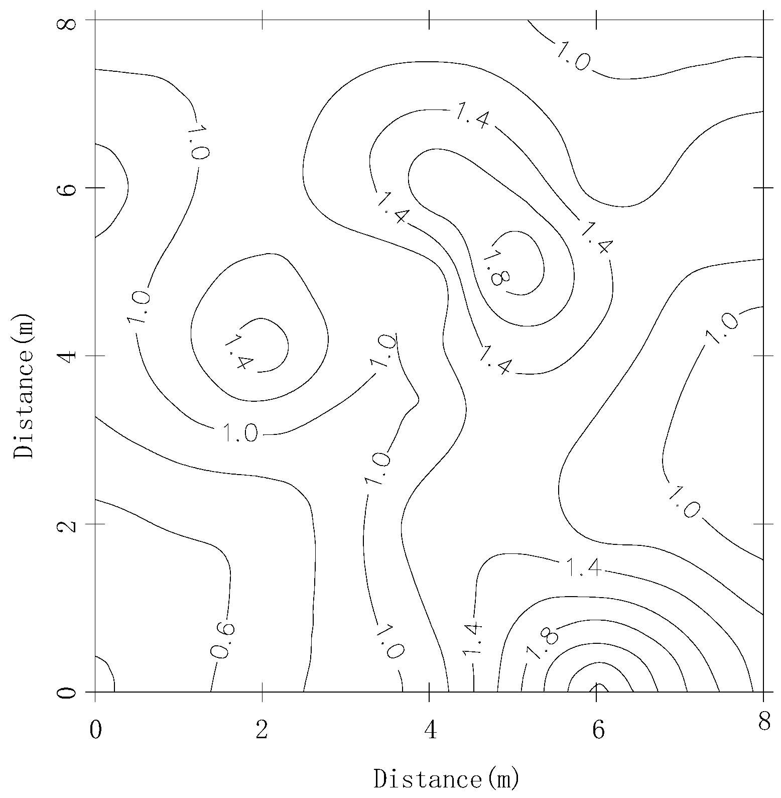
Zavattaro et al. [22] measured near-saturated hydraulic conductivity in a 8 × 8 m plot on a silt loam soil at Säby, in east central Sweden, to investigate the spatial dependence of near-saturated hydraulic conductivity. In total, 37 measurement locations were located on the plot. The variability was represented by a single parameter, the scale factor ${\delta }_i$, following the Miller and Miller similar media theory, based on which the saturated conductivity is scaled with the scale factor:

$$K_{si}=K_{\mathrm{ref}}\times {\delta }_i^2,$$

(17)

where $K_{\mathrm{ref}}$ is the reference value of the plot, which is equal to 30.9 cm/h in the plot, and i refers to each location. The contour map of the scale factor is shown in Figure 2.

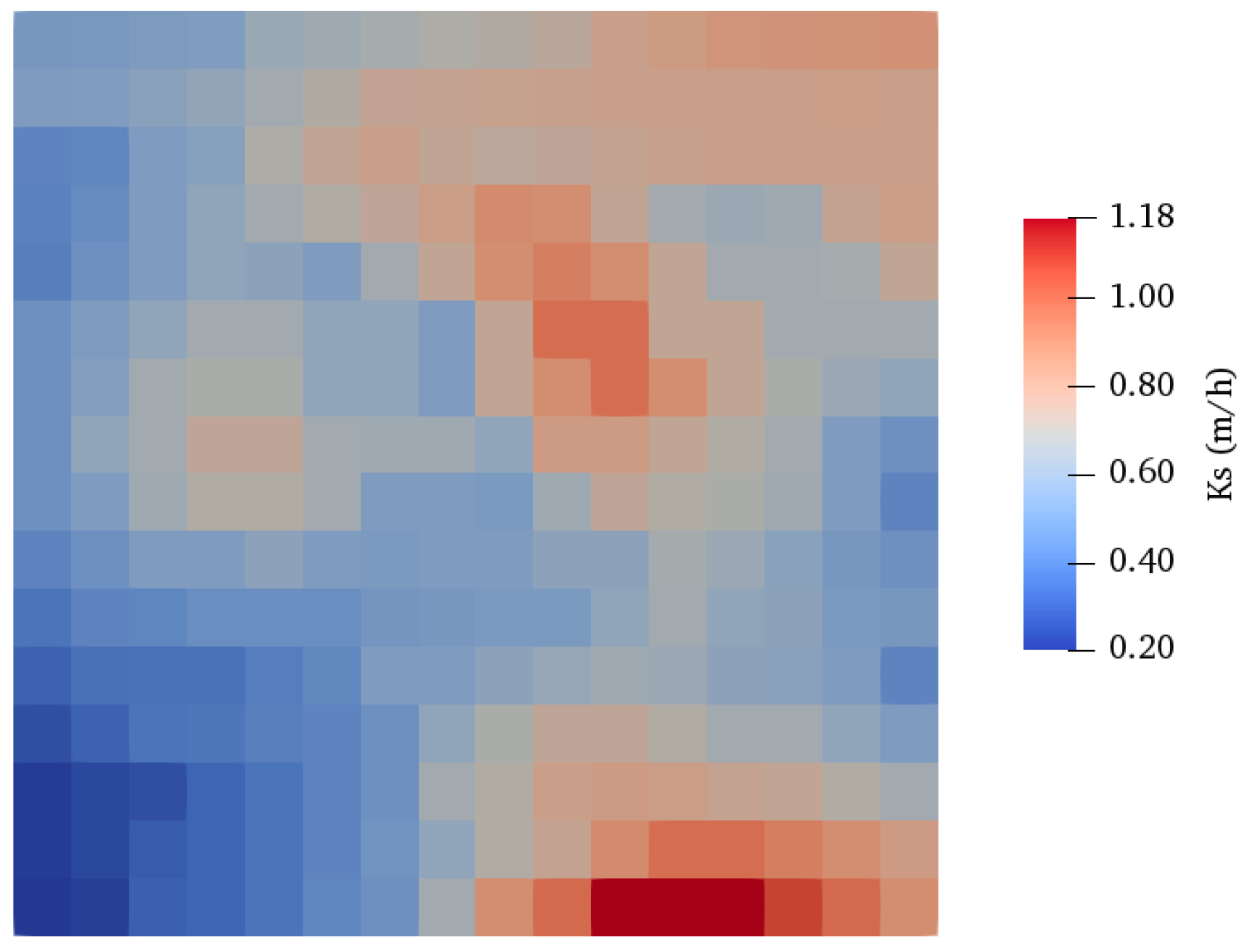
The plot surface was divided into a grid of 16 rows and 16 columns, each square is 0.5 × 0.5 m in size, and the hydraulic conductivity of each square is represented by that at the midpoint of the small square, which is obtained by interpolation. Thus, each square corresponds to a soil column, and the thickness of the soil layer is 3 m. The distribution of hydraulic conductivity in ParaView is shown in Figure 3.

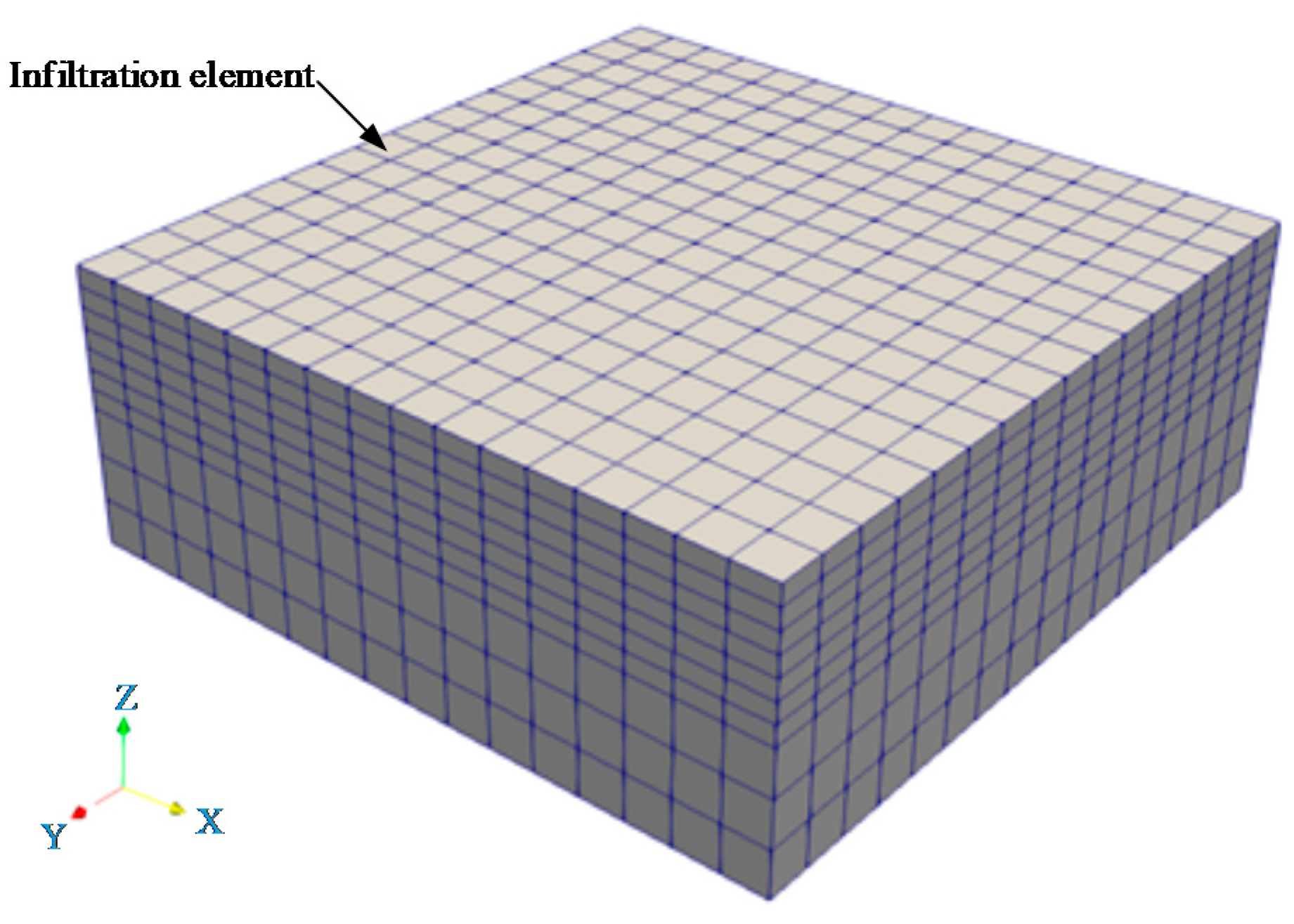
The established model is shown in Figure 4. To focus on the initial infiltration, the upper part of the model has a finer mesh than lower part. The boundary conditions are specified as follows: for top surface, saturation is set to 1.0 at t = 0, and for four side surfaces, symmetry boundary is set. The initial water content ${\theta }_{\mathrm{i}}$ is set to 0.12 for the whole soil body.

To model rainwater infiltration, the VG equation proposed by van Genuchten in 1980 is used [23] with the expression as below

$$\theta \left(h\right)=\{\begin{array}{ll}{\theta }_r+\frac{{\theta }_s-{\theta }_r}{{\left[1+{\left(\alpha \left|h\right|\right)}^n\right]}^m}\hfill & ifh<0\hfill \\ {\theta }_s\hfill & otherwise\hfill \end{array},$$

(18)

where $\theta$ is the soil water content, ${\theta }_r$ is the soil residual water content, ${\theta }_r$ = 0.067, ${\theta }_{\mathrm{s}}$ is the soil saturated water content, ${\theta }_{\mathrm{s}}$ = 0.45, h is soil water potential, α is a scale parameter inversely proportional to mean pore diameter, α = 0.49 cm⁻¹, n and m are the shape parameters of soil water characteristic, n = 1.578, m = 1 − 1/n. However, as expressed in Equations (5) and (6), the Brooks and Corey model is used in the above theoretical derivation. The parameters used by the two models are not the same. Hence, the parameters in Brooks and Corey are converted from those of the VG model according to the equivalent conversion method proposed by Hubert J. Morel-Seytoux [24].

4.2. Results Comparison

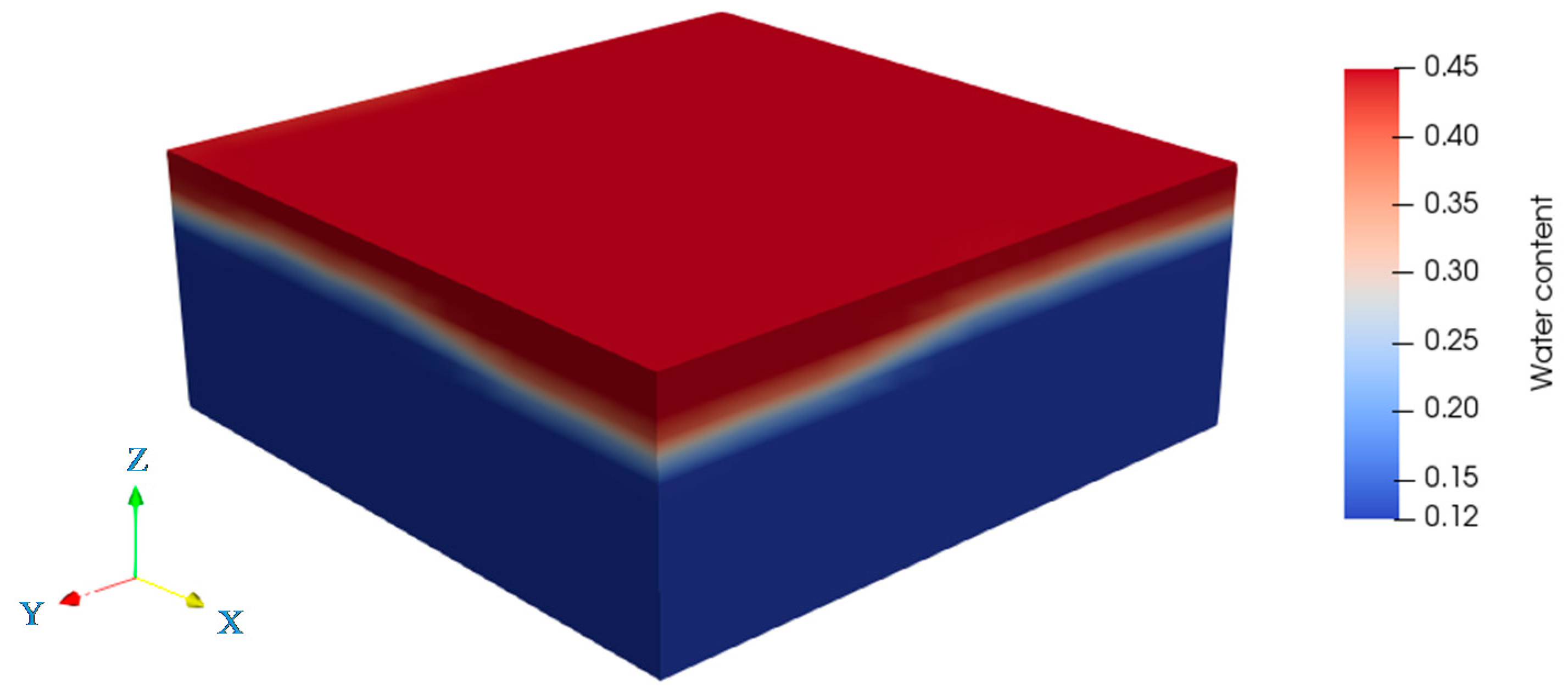
The simulation of rainwater infiltration is completed by suGWFoam, and the spatial distributions of water content in the plot at different times are obtained. Figure 5 shows the water content distribution at t = 0.5 h displayed in ParaView.

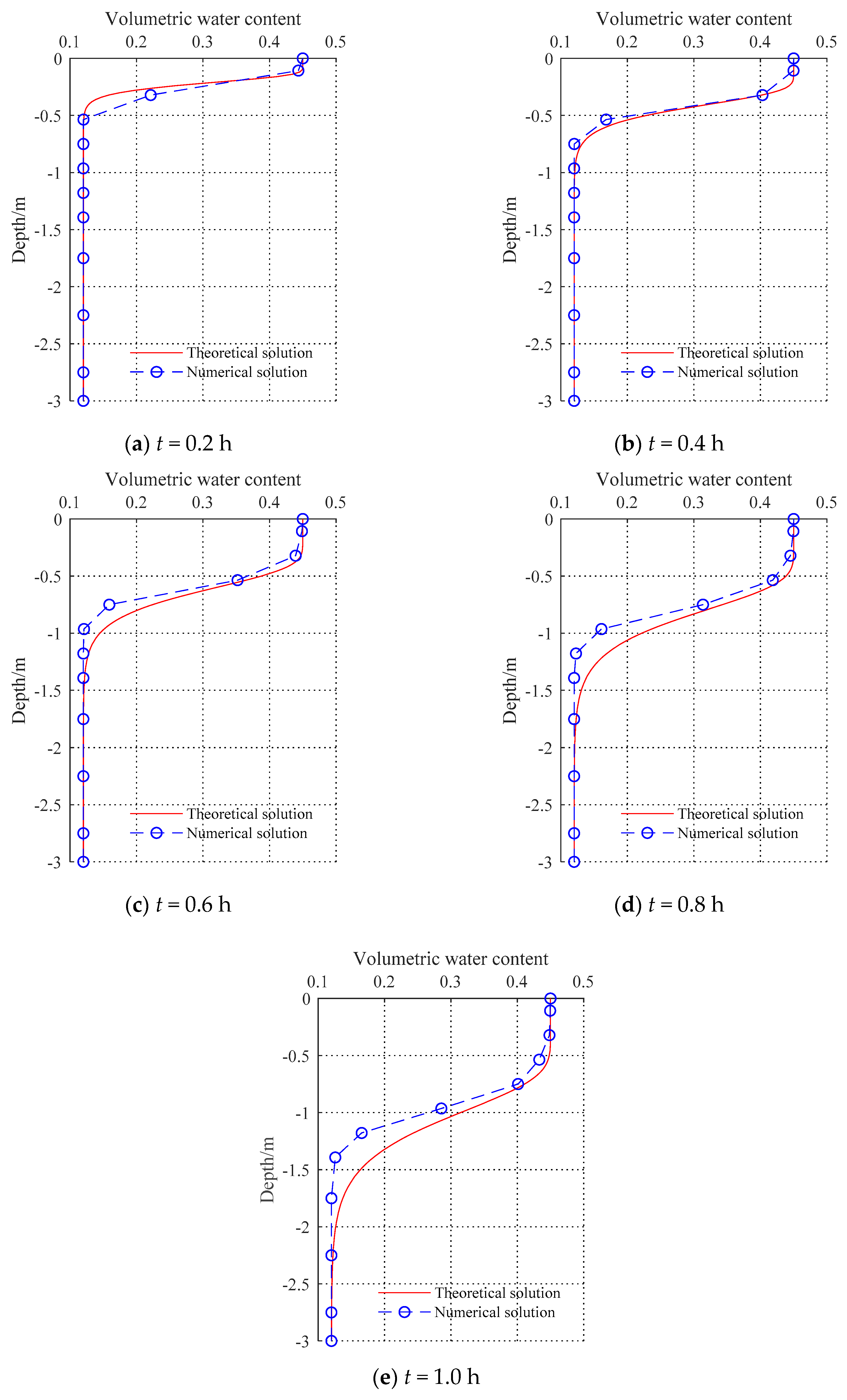
Result comparisons between the theoretical calculation and numerical simulation at different times are shown in Figure 6.

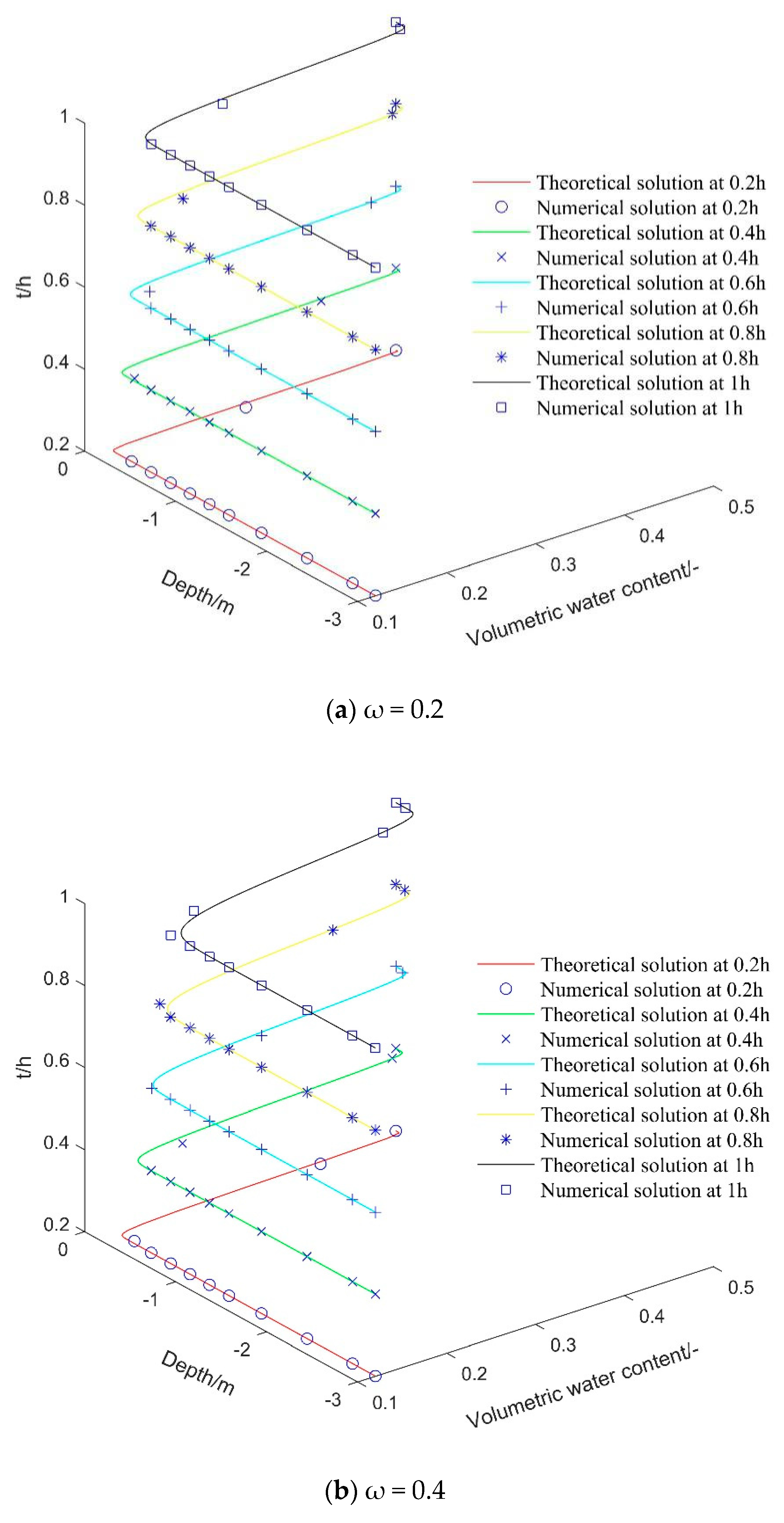
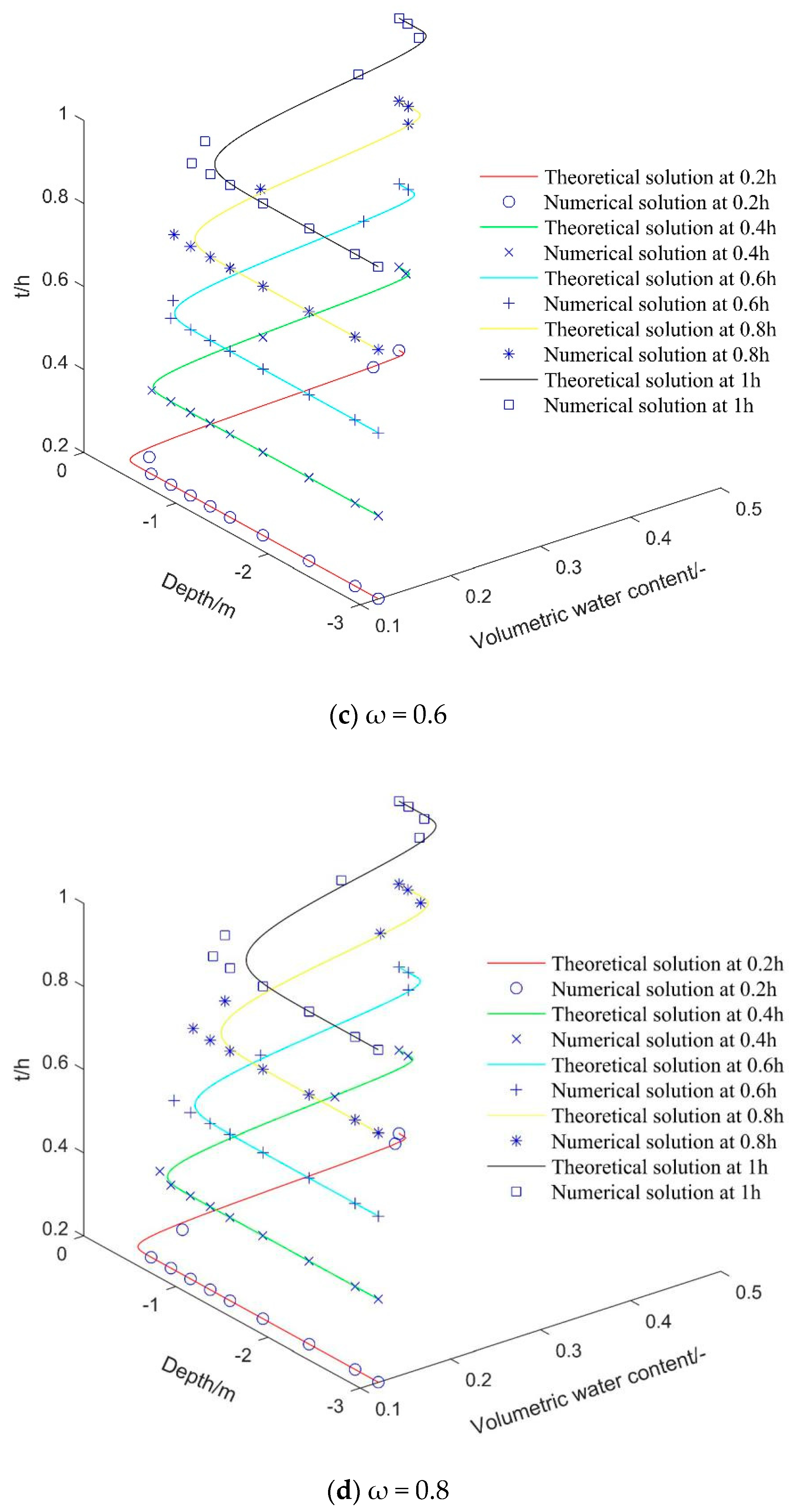
Due to the uncertainty of the hydraulic conductivity in the random field, we performed multiple simulations. In each simulation, the original hydraulic conductivity was multiplied by a proportional coefficient ω, so that different probability distributions of K_s were verified. The calculation results are shown in Figure 7.

As can be seen in above figures, the difference between the numerical solution and theoretical solution is small, which shows that the previous theoretical derivation can be used to calculate rainwater infiltration under heavy rainfall conditions.

5. Slope Stability Analysis

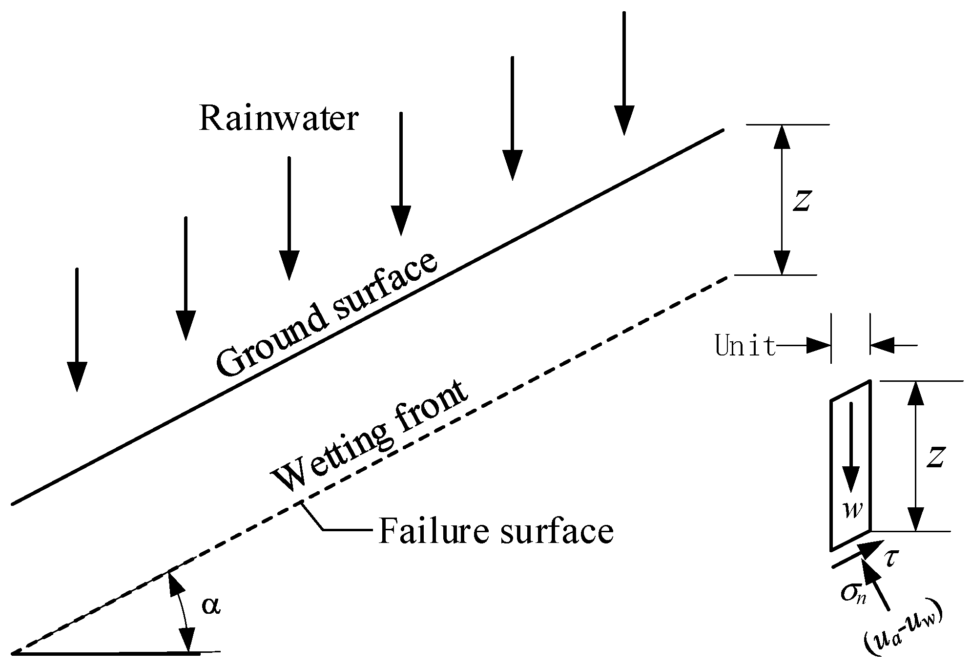
The rainfall-induced landslides [25,26] generally take the form of shallow (typically 1–3 m deep), translational slides, which form parallel to the original slope surface. A great deal of research shows that the potential slip surface of the infinite slope is almost always coincident with the surface of the wetting front. In the paper, the infinite slope model is used to represent shallow landslides induced by rainfall, as shown in Figure 8.

The limit equilibrium method can be readily applied to calculate the factor of safety. The shear resistance of the soil slice can be determined using the modified Mohr–Coulomb failure criterion [27,28] for unsaturated soil:

$${\tau }_f=c\prime +\left({\sigma }_n-u_a\right)\tan \phi \prime +\left(u_a-u_w\right)\tan {\phi }^b,$$

(19)

where c′ is the effective cohesion, φ′ is the effective angle of friction, $\tan {\phi }^b$ is the change rate of shear strength with matrix suction, ${\sigma }_{\mathrm{n}}$ is the total normal stress on the failure plane, $u_a$ is the pore-air pressure on the failure plane, $u_w$ is the pore-water pressure on the failure plane, $\left({\sigma }_n-u_a\right)$ is the net normal pressure on the failure plane, $\left(u_a-u_w\right)$ is the matric suction on the failure plane, and ${\phi }^b$ is the angle that defines the shear strength increases with an increase in matric suction.

The factor of safety for homogeneous infinite soil slope can be written as:

$$F_s=\frac{{\tau }_f}{{\tau }_m}=\frac{c\prime +\left({\sigma }_n-u_a\right)\tan \phi \prime +\left(u_a-u_w\right)\tan {\phi }^b}{z\gamma \cos \alpha \sin \alpha },$$

(20)

where γ is the unit weight of soil, z is the depth of the wetting front during infiltration process, and $\alpha$ is the slope angle.

Vanapalli et al. [29] determined the relationship between ${\phi }^b$ and the relative volumetric water content s through a micro-analysis of unsaturated soil.

$$\tan {\phi }^b=s\cdot \tan \phi \prime ,$$

(21)

We adopt the fitting formula proposed by Brook and Corey [30] to determine the relationship between the water content and the matric suction:

$$\psi \left(s\right)={\psi }_b\cdot s^{-1/\lambda },$$

Thus, Equation (20) can be rewritten as:

$$F_s=\frac{\tan \phi \prime }{\tan \alpha }+\frac{c\prime -{\psi }_b{\gamma }_w{s}^{1-\frac{1}{\lambda }}\tan \phi \prime }{z\gamma \sin \alpha \cos \alpha },$$

(22)

where ${\gamma }_w$ is the unit weight of water. Note that the safety factor of slope is related with the depth of the wetting front and the water saturation, which are functions of the saturated hydraulic conductivity of soils and the rainfall duration. Thus, the safety factor of the slope varies with time during rainfall, and is affected by the hydraulic conductivity of soils.

In addition, owing to rainwater infiltration into the soil, the weight of the soil also increases, which is expressed as:

$${\gamma }_t=\gamma +\Delta \theta \cdot {\gamma }_w,$$

(23)

where ${\gamma }_t$ is the unit weight of soil at time t, and $\Delta \theta$ is the increase in volumetric water content. Substitute the expression of the increase in volumetric water content $\Delta \theta ={\theta }_i+\left({\theta }_s-{\theta }_r\right)\left(s_t-s_i\right)$ into Equation (23), the unit weight of the soil can be rewritten as:

$${\gamma }_t=\gamma +{\gamma }_w\cdot \left[{\theta }_i+\left({\theta }_s-{\theta }_r\right)\left(s_t-s_i\right)\right],$$

(24)

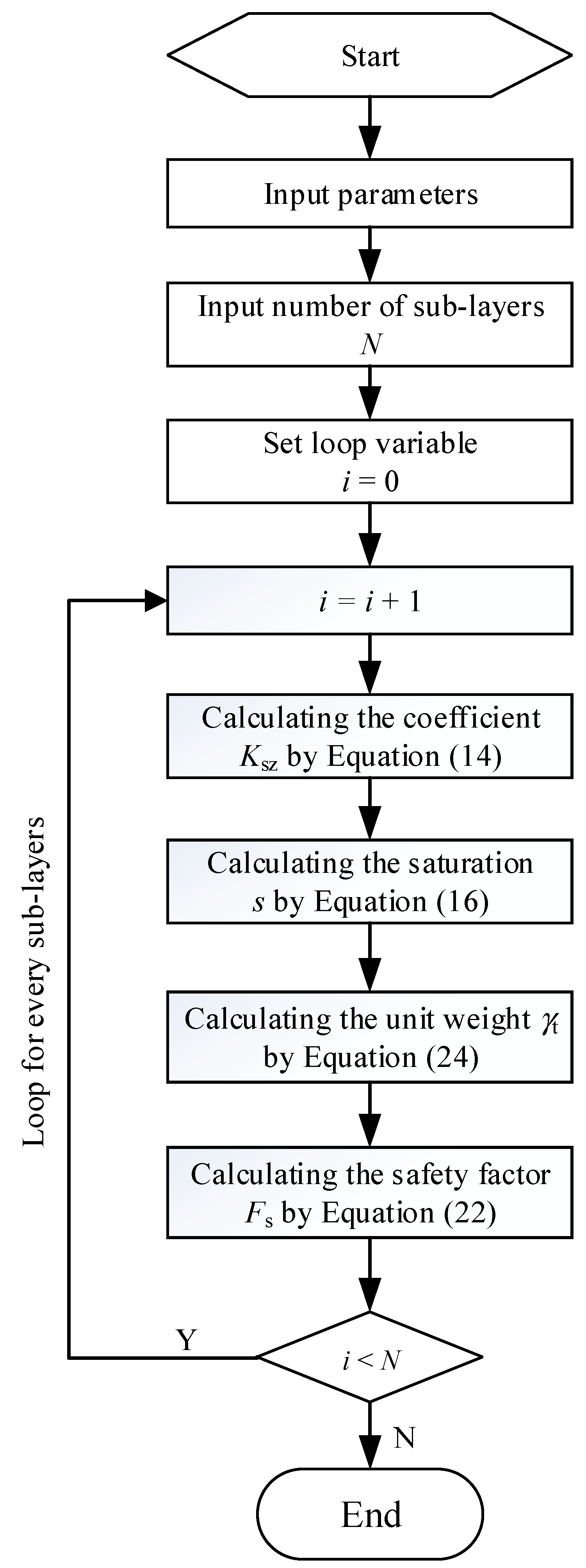
Throughout the preceding discussion, the safety factor of the slope can be evaluated, and the corresponding solution procedure is shown in Figure 9.

6. Case Study

A hypothetical natural unsaturated soil slope, whose surface was covered by a layer of 1.0 m thick sandy clay loam, was adopted as an example, and the slope angle is equal to 30 degrees. The soil is uniformly dry, and the soil surface was held to be saturating at the beginning of the infiltration. Some of parameters are summarized in

Table 2. Parameters for the study case.

Parameters	Definition	Value
$K_{\mathrm{s}}$	Saturated hydraulic conductivity	${\mu }_{K_{\mathrm{s}}}=0.43\mathrm{cm}/\mathrm{h}$
${\theta }_{\mathrm{s}}$	Saturated volumetric water content	0.398
${\theta }_r$	Residual volumetric water content	0.068
${\theta }_i$	Initial volumetric water content	0.148
${\psi }_b$	Air entry value	0.2809 m
λ	Pore distribution index	0.25
${\gamma }_d$	Unit dry weight of soil	16.5 kN/m3
c′	Effective cohesion	3.0 kPa
φ′	Effective angle of internal friction	18°

[31]. Among them, only the saturated hydraulic conductivity was treated as a random variable obeying lognormal distribution, and the mean ${\mu }_{K_{\mathrm{s}}}$ of the saturated hydraulic conductivity was fixed.

6.1. Rainfall Duration

Infiltration is a process in which rainwater falling to the ground surface enters the soil. In general, the longer the infiltration time, the more rainwater seeps into the soil. At the same time, the infiltration is affected by the variability of hydraulic conductivity, and is not distributed evenly in the whole field. In this section, the influence of rainfall duration on rainwater infiltration and the corresponding safety factor under the condition of variation of hydraulic conductivity is discussed. To this end, for a specific soil hydraulic conductivity mean and coefficient of variation, the changes of water content in the soil and the corresponding safety factor are calculated with time increase. Many factors affect the variability of soil saturated hydraulic conductivity, which varies in a larger range. The in-situ test data collected by Duncan [5] shows that the coefficient of variation of the saturated hydraulic conductivity ranges from 68–90%, as shown in Table 1. By analyzing a lot of soil samples of a loess slope from the South Jingyang Plateau, northwest China, Wei Wang [32] concluded that $K_{\mathrm{h}}$ and $K_{\mathrm{v}}$ measurements of the loess samples collected in the trench and adit all show log-normal distribution, and the hydraulic conductivity varied between 53% and 114%. In the case study, the coefficient of the variation of the saturated hydraulic conductivity (CoV) takes 60%.

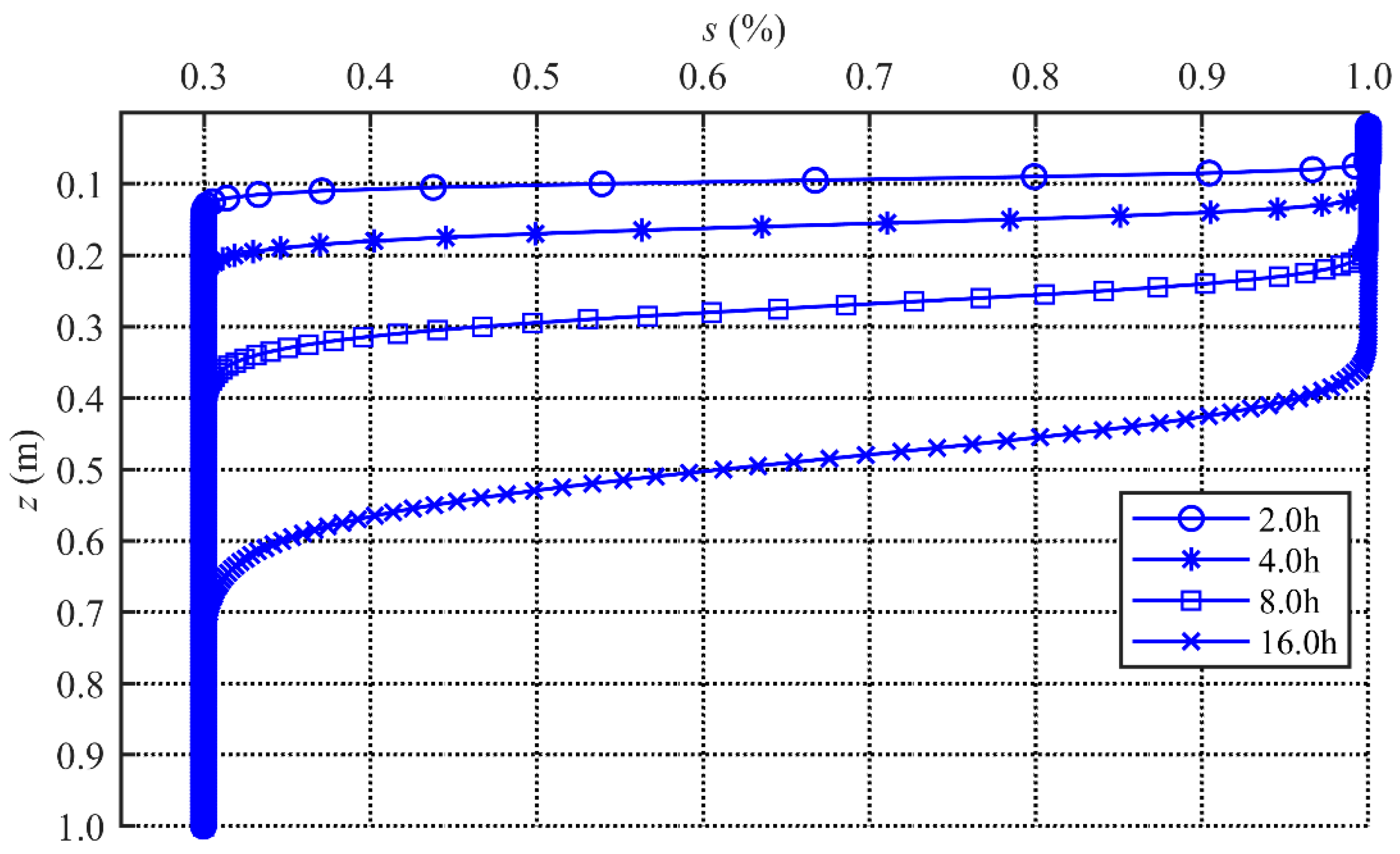
Changes in saturation (denoted by s) can intuitively reflect the infiltration process of rainwater. The saturation profiles at different times are plotted in Figure 10, and clearly show the process of rainwater infiltration. At time t = 2.0 h, the infiltration distance is about 0.1 m. At time t = 4.0 h, the infiltration distance is about 0.15 m. At time t = 8 h, the infiltration distance is about 0.25 m. At time t = 16.0 h, the infiltration distance is about 0.5 m. It is obvious that the infiltration distance increases with time, and the infiltration rate decreases significantly over time. On the other hand, it also can be seen that the saturation profiles have an extended leading portion at deeper locations, and as time increases, the leading edge of the saturation profiles is longer. This is because the rainwater moves faster at those elements of larger K_s value, which results in the differences between different infiltration elements, and the differences will grow bigger with time. The distribution of the wetting fronts of all infiltration elements determines the shape of the saturation.

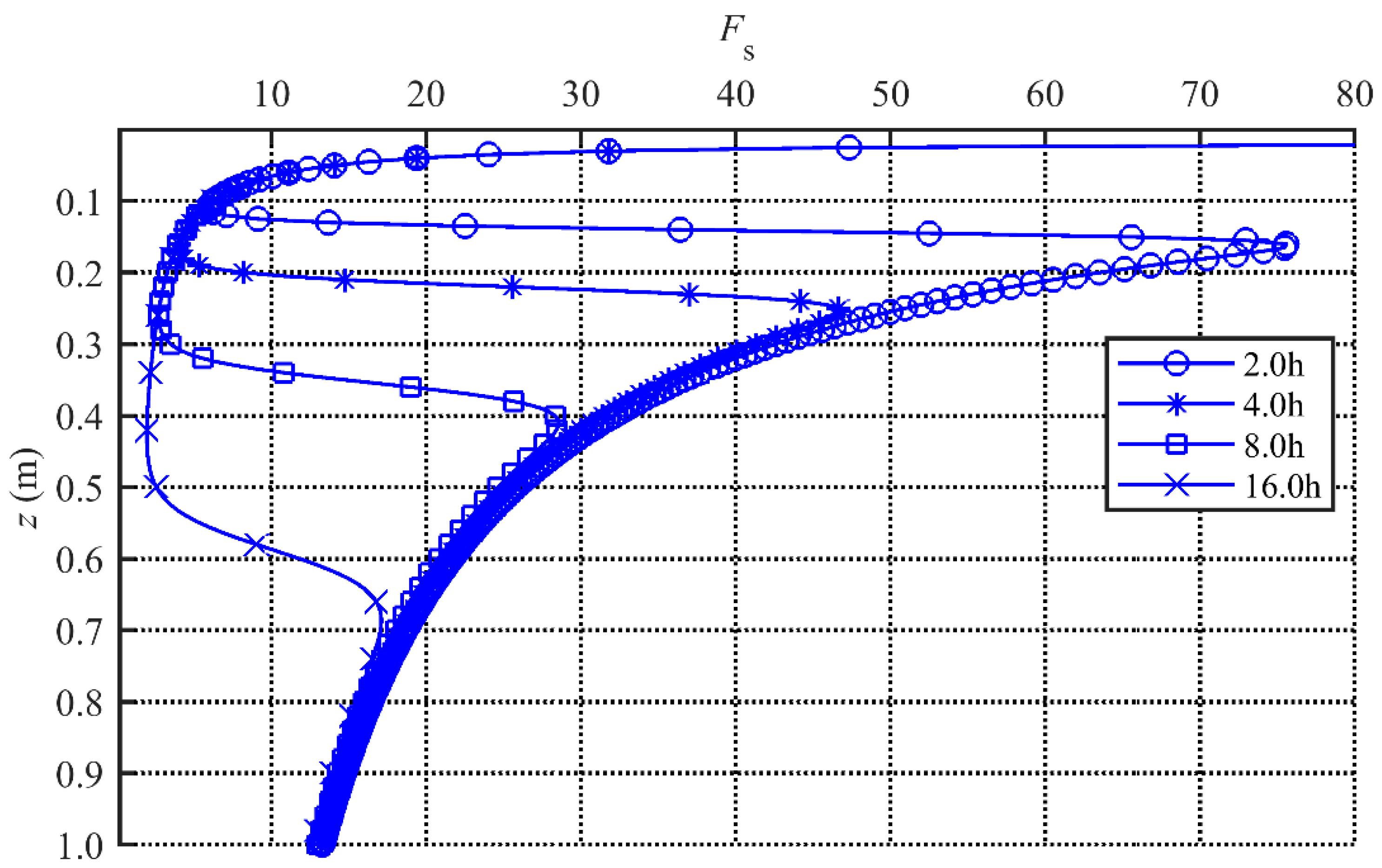
Figure 11 shows the safety factor (denoted by F_s) profiles at different times. It can be seen that the safety factors decrease with depth in the shallower ground, then increase below the wetting fronts. Therefore, there is a minimum safety factor near the surface at different times, which explains the reason why the shallow landslide occurs during rainfall. This is because the water content decrease with rainfall infiltration above the wetting front, which induces a decrease in matrix suction, and the corresponding decrease in safety factors, and below the wetting front the water content remains the same as the initial value. Subsequently, as depth increases, the soil saturation does not change much. Accordingly, the contribution of the matrix suction to the safety factor also does not change much. Meanwhile, owing to the increase in soil weight, the safety factor continues to show a decreasing trend with depth increase, as shown in Equation (22). Minimum safety factor value is reached at the bottom. It also shows that the potential slide plane is not always coincident with the wetting front, and sliding may also occur at the bottom along the bedrock plane. The wetting front and the bedrock plane are two potential sliding planes that need to be taken into account, and Ma et al. [33] discusses the problem for an infinite slope.

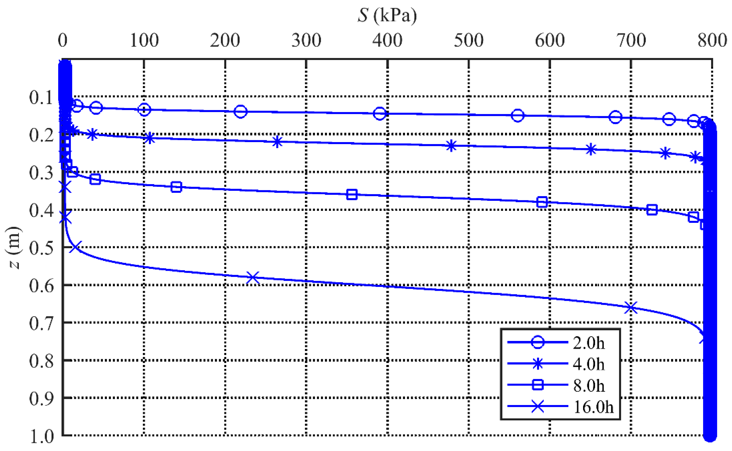
When rainfall duration lasts a longer time, like time t = 16 h as shown in Figure 11, the decrease in safety factors at the wetting front is not obvious at this time compared with other times. At the depth of about 0.5 m, the local minimum safety factor occurs. As the depth further increases, the contribution of matrix suction to the safety factor gradually increases; correspondingly, the safety factor increases slowly. This is because the water content has a slow change with depth, and matrix suction also has a corresponding process with depth. To illustrate this point, the matrix suction profiles at different times are plotted in Figure 12, in which it can be seen that the matrix suction is about 800 kPa corresponding to the initial water content. With rainfall infiltration, the water content of soil above the wetting front increases, and the corresponding matrix suction decreases. For a shorter time period, the shorter the time, the steeper the change in the matrix suction along depth, as shown in Figure 12. At the time t = 16 h, the change in the matrix suction with depth is slower, which is consistent with the saturation profile in Figure 10, and induces the formation of the safety factor profile in Figure 11.

6.2. Coefficient of Variation

The coefficient of variation, also known as “relative variability,” is equal to the standard deviation of a distribution divided by its mean, and represents the spatial variability of soil saturated hydraulic conductivity. A larger coefficient of variation indicates higher spatial variability of the saturated hydraulic conductivity. In this section, the coefficient of variation was chosen to be 20%, 50%, 80% and 150%, respectively, in order to evaluate the influence of the variability of hydraulic conductivity on rainwater infiltration and the safety factor of the slope.

6.2.1. Saturation

Rainfall infiltration into soil leads to an increase in saturation. In this section we will discuss how the variability of hydraulic conductivity affects the change in soil saturation.

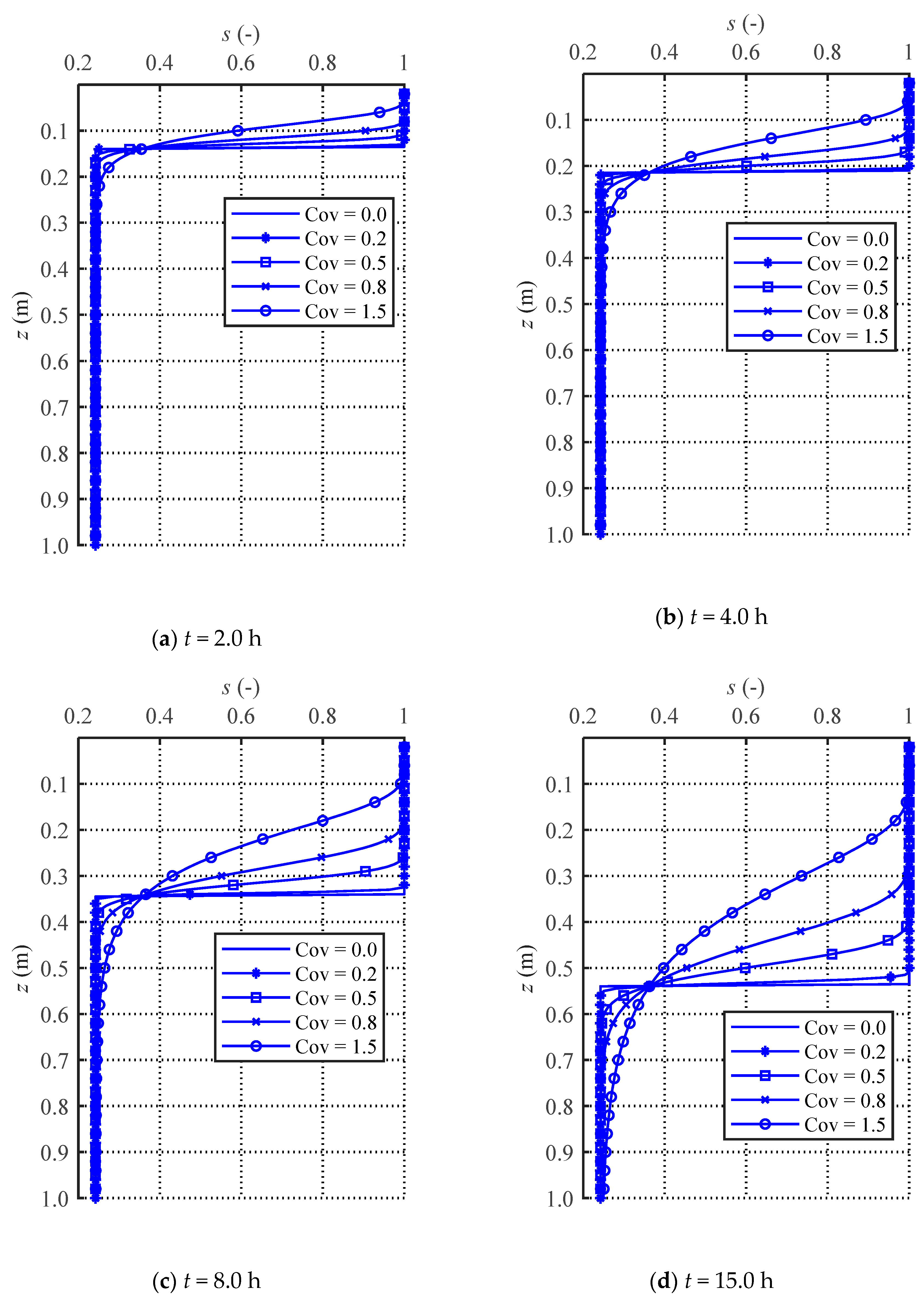
Figure 13 shows the saturation profiles under different variability of hydraulic conductivity conditions at different times. For comparison, coefficient of variation CoV = 0 is also considered, representing a uniform soil layer. From Figure 13, it is seen that the smaller the coefficient of variation, the more obvious the change in saturation. For example, the saturation profile of uniform soil layer has a right angle at the wetting front, indicating a steep decrease in saturation, and the saturation profile with a coefficient of variation of 1.5 is the slowest in change of saturation along depth from the top to the bottom of the slope. This is because the smaller the CoV of the saturated hydraulic conductivity, the more uniform the soil in the horizontal layer is; likewise, the smaller the difference of the saturated permeability coefficient is, the easier it is to achieve synchronous infiltration between different soil cube elements. This is consistent with the results of numerical simulations by Chen et al. [20].

6.2.2. Safety Factor

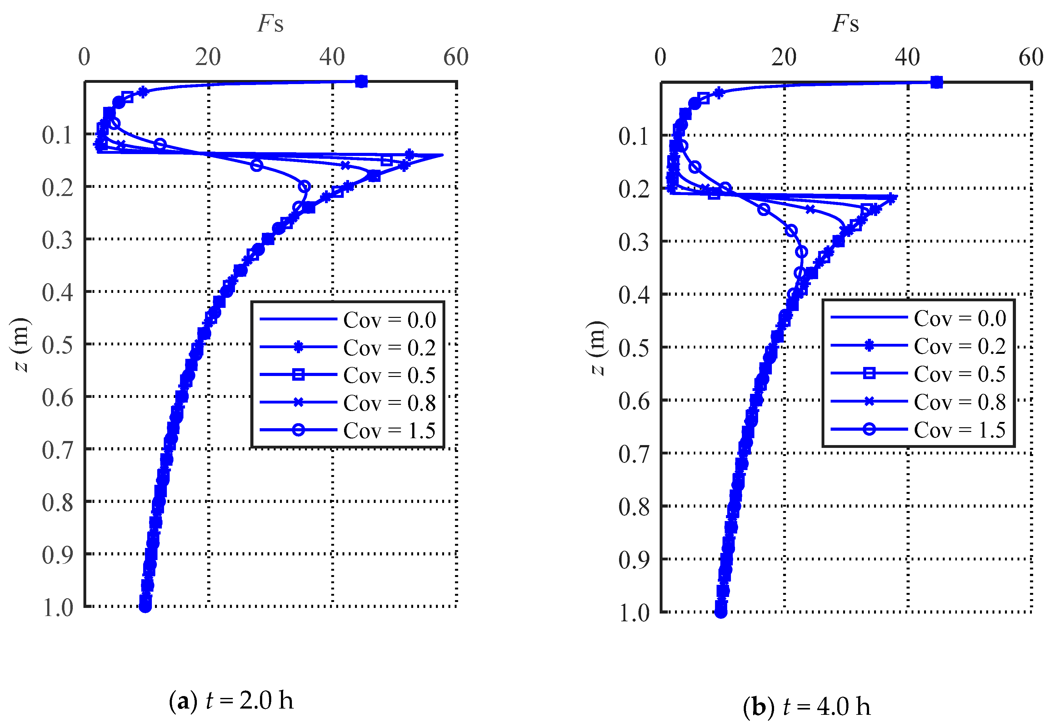
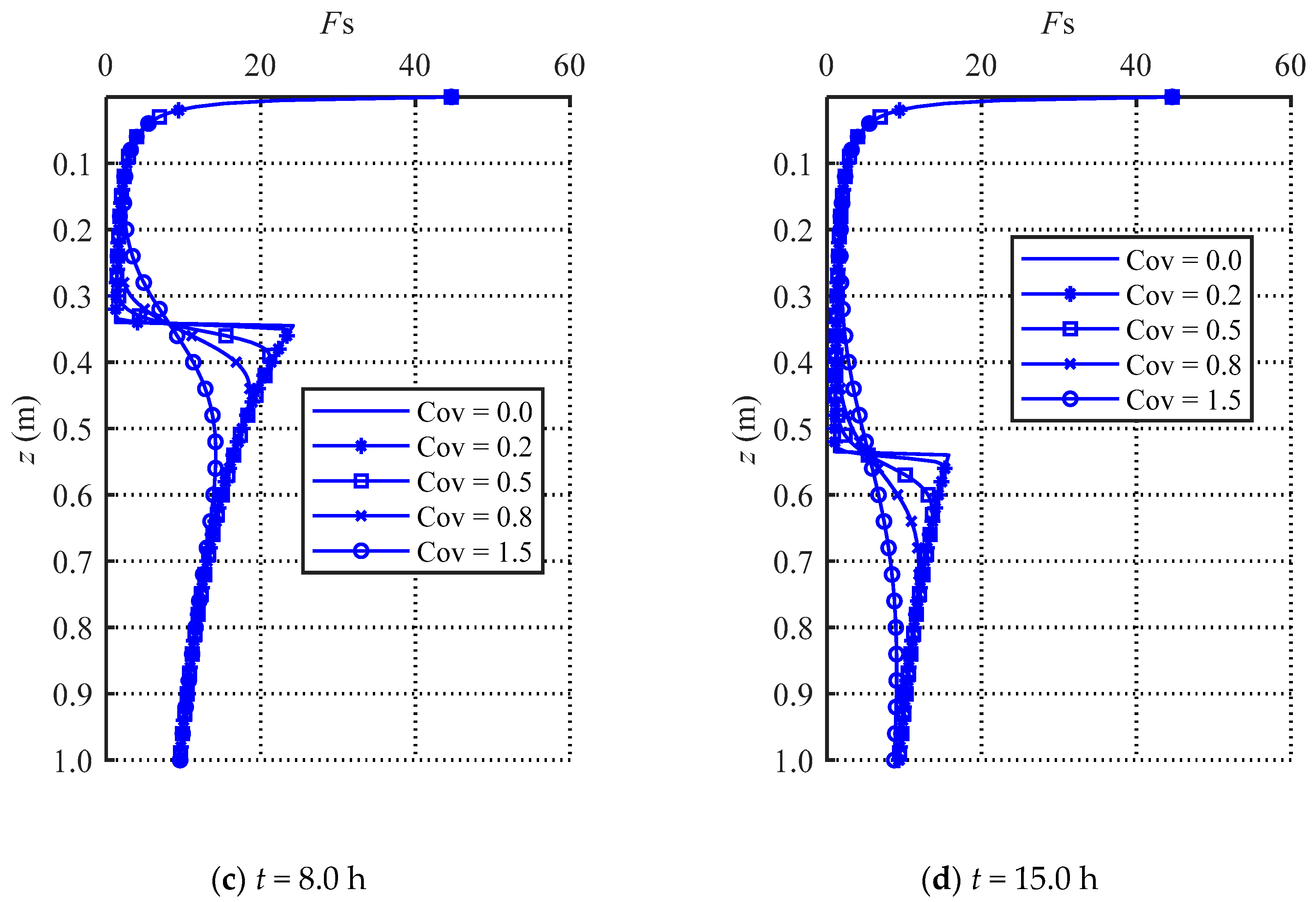
Rainfall infiltration induces an increase in water content, which adversely affects the stability of a slope. How the variability of hydraulic conductivity affects the change in safety factor of a slope is discussed in this section. The safety factor profiles under different variability of hydraulic conductivity conditions at different times are shown in Figure 14. It can be seen that the smaller the coefficient of variation of the saturated hydraulic conductivity, the smaller the safety factor at the corresponding wetting front, and the higher the increase in safety factor below the wetting front. By contrast, the larger the coefficient of variation, the smaller the safety factor at the corresponding wetting front, and the less obvious the increase in the safety factor below the wetting front. In particular, when the coefficient of variation is 1.5, the slope safety factor decreases monotonously from the top to the bottom of the slope, which is different from other coefficients of variation. This corresponds to the distribution of saturation at different times. The smaller the coefficient of variation, the higher the saturation above the wetting front. The lower the corresponding matrix suction of soil, and the smaller the safety factor of the slope at the wetting front. Similarly, the lower the saturation below the wetting front, the higher the corresponding matrix suction of soil, and the greater the safety factor of the slope. On the other hand, the larger the coefficient of variation, the smoother the curve of the saturation profile, and the lower the saturation above the wetting front, the higher the corresponding matrix suction, and the higher the safety factor of the slope, so that below the wetting front the change of saturation is not obvious, the corresponding change of matric suction is also not obvious, and the change in safety factor of the slope is slow.

From the perspective of slope stability, It can be concluded that in the early stage of rainfall, such as time t = 2 h or t = 4 h in this example, the smaller the coefficient of variation, the smaller the corresponding safety factor, and the higher the slope instability probability. In the late stage of rainfall, for example, at time t = 15 h in this example, the difference in safety factor is not significant for different coefficients of variation, because at this time the upper part of the soil layer is saturated regardless of the coefficient of variation.

6.2.3. Cumulative Infiltration

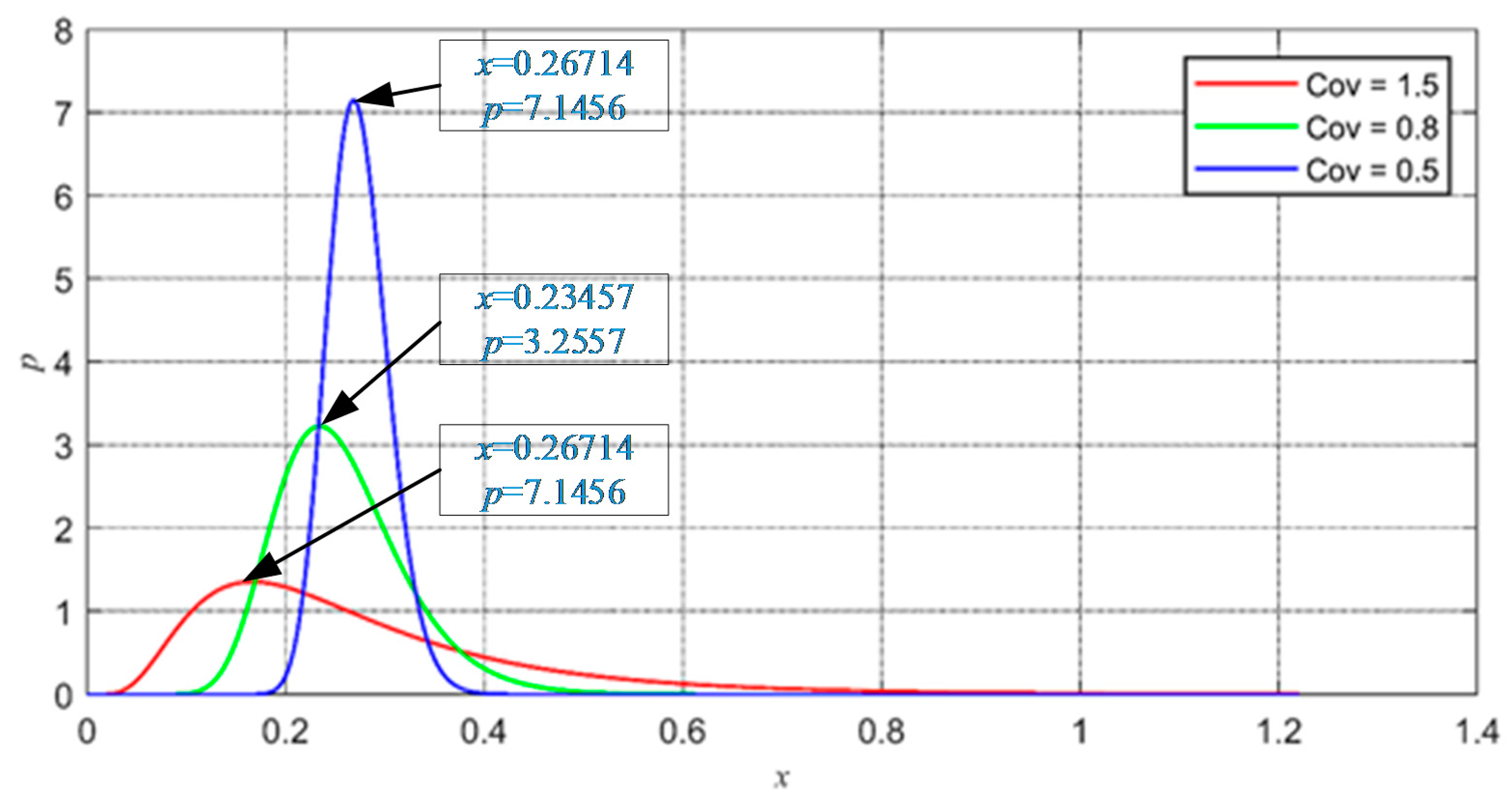
The safety factor of the slope is related to antecedent accumulative infiltration. Figure 15 shows the variation of cumulative infiltration with time under different coefficients of variation. With increase in time, the cumulative infiltration gradually increases. At the same time, the larger the coefficient of variation, the smaller the corresponding cumulative infiltration. When the coefficient of variation is 0.2, the cumulative infiltration is close to the cumulative infiltration under uniform infiltration, i.e., variation coefficient equals zero. With the increase of the coefficient of variation, the difference of cumulative infiltration is also increasing. When the coefficient of variation reaches 1.5, the difference in cumulative infiltration is significant. This is because when the coefficient of variation becomes larger, the difference in the coefficient of hydraulic conductivity among the cube elements also becomes larger, which affects the cumulative infiltration. Figure 16 shows the curves of the probability density function for different coefficients of variation. It can be clearly seen from the curves that when CoV = 0.5, the average value of saturated hydraulic conductivity is about 2.59 cm/h, and the PDF curve is basically symmetrical with the average value. That is, the number of saturated hydraulic conductivity for the cube infiltration elements above the average and below the average is substantially equal, in which case the accumulative infiltration is close to the cumulative infiltration under uniform soil condition. As the coefficient of variation increases, the average value shifts significantly to the left, meaning that the generated saturated hydraulic conductivity is much less than the average value, and the larger the coefficient of variation, the more obvious this trend is. Therefore, under the assumption of lognormal distribution of saturated hydraulic conductivity, the higher coefficient of variation has a negative impact on the cumulative infiltration.

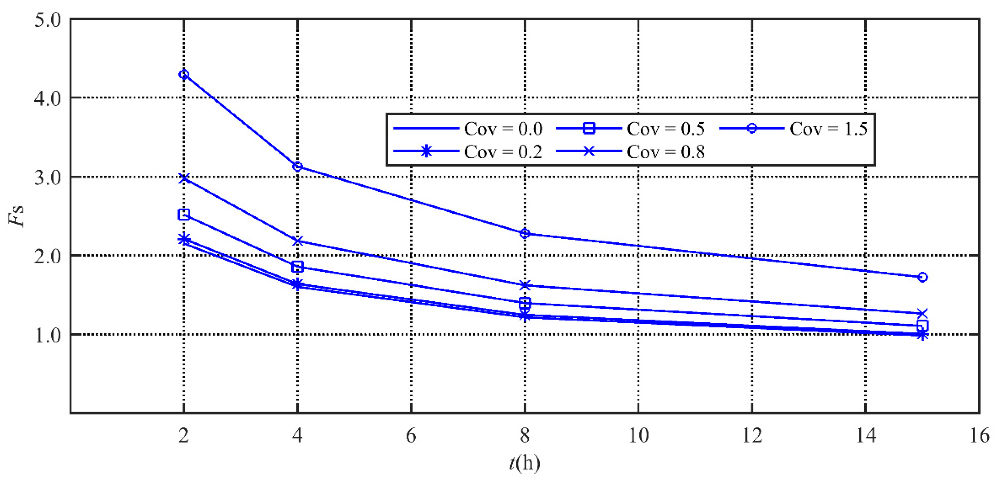
As stated above, the difference in coefficient of variation leads to a difference in the accumulative infiltration during the same period of time, and this difference also leads to different slope stability. The variation of safety factors at the wetting front with time are shown in Figure 17. It can be seen that at the same time, the larger the coefficient of variation, the higher the corresponding safety factor, which is consistent with the water content distribution along depth, because the larger the coefficient of variation, the smoother the curve of the saturation profile. By contrast, the lower the coefficient of variation, the higher the saturation at the wetting front, and the lower the matrix suction, which results in a smaller safety factor. In addition, as time increases, the safety factor decreases, and the difference between the safety factors corresponding to a different coefficient of variation is also smaller. This is due to the fact that when the rainwater infiltrates for a certain period of time, regardless of the coefficient of variation, the upper soil is almost completely saturated, as shown in Figure 13d, resulting in an increasingly small difference in safety factors.

7. Conclusions

By improving and simplifying the GA model, this paper deduces the analytical formula of the failure probability of the infinite slope under heavy rainfall conditions, and quantitatively analyzes the influence of the horizontal variability of saturated hydraulic conductivity on the slope stability. Finally, some conclusions are summarized as follows.

(1)

For a certain coefficient of variation, there is a local minimum at the wetting front in the initial period of the rainfall and, as time increases, the reduction of the safety factor at the wetting front becomes insignificant until it disappears.

(2)

At the initial stage of rainfall, the smaller the coefficient of variation, the more rainwater is concentrated in the upper part of the soil layer, and the smaller the safety factor. With the increase of time, the influence of the change in coefficient of variation on slope stability becomes less significant in the later period of rainfall.

(3)

There are two potential slip surfaces due to the influence of matrix suction and the increase in soil weight with depth. In general, with the increase of depth, the safety factor gradually decreases, and the safety factor at the bottom of the weathered layer is the lowest. Thus, the bottom is a potential sliding surface. The above discussions show that in the early stage of rainfall, there is a significant reduction of the safety factor at the wetting front. Therefore, the wetting front is also a potential sliding surface, which is caused by sudden changes in matrix suction induced by rainfall infiltration.

(4)

The high coefficient of variation of hydraulic conductivity has a negative impact on the cumulative infiltration of rainwater. The larger the coefficient of variation, the lower the cumulative infiltration. Correspondingly, the larger the coefficient of variation, the higher the safety factor at the initial stage of rainfall. Meanwhile, with the increase of time, the difference between the safety factors corresponding to coefficients of variation is becoming increasingly small.

The effect of slope angle on rainwater infiltration was neglected. The effect is complicated by many confounding factors [34], and due to the current technology level and theory, the main influence is ambiguous, which may result in a contradictory view. In addition, the results show that hydraulic conductivity has an impact on rainwater infiltration and corresponding slope stability. Thus, in slope stability analysis, special attention should be paid to the variability of hydraulic conductivity.

References

- Chae, B.G.; Lee, J.H.; Park, H.J.; Choi, J. A method for predicting the factor of safety of an infinite slope based on the depth ratio of the wetting front induced by rainfall infiltration. Nat. Hazards Earth Syst. Sci. 2015, 15, 1835–1849. [Google Scholar] [CrossRef] [Green Version]
- Zhang, S.; Tang, H.M.; Liu, X.; Tan, Q.W.; Xia-hou, Y.S. Seepage and Instability Characteristic of Slope Based on Spatial Variation Structure of Saturated Hydraulic Conductivity. Earth Sci. 2018, 43, 622–634. [Google Scholar]
- Zhu, H.; Zhang, L.M.; Zhang, L.L.; Zhou, C.B. Two-dimensional probabilistic infiltration analysis with a spatially varying permeability function. Comput. Geotech. 2013, 48, 249–259. [Google Scholar] [CrossRef]
- Bai, T.; Huang, X.M.; Li, C. Slope stability analysis considering spatial variability of soil properties. J. Zhejiang Univ. 2013, 47, 2221–2226. [Google Scholar]
- Duncan, J.M. Factors of safety and reliability in geotechnical 47, 2221–2226.engineering. J. Geotech. Geoenviron. Eng. 2000, 126, 307–316. [Google Scholar] [CrossRef]
- Phoon, K.K.; Kulhawy, F.H. Characterization of geotechnical variability. Can. Geotech. J. 1999, 36, 612–624. [Google Scholar] [CrossRef]
- Kulhawy, F.H. On the evaluation of soil properties. ASCE Geotech. Spec. Publ. 1992, 31, 95–115. [Google Scholar]
- Benson, C.H.; Daniel, D.E.; Boutwell, G.P. Field performance of compacted clay liners. J. Geotech. Geoenviron. Eng. 1999, 125, 390–403. [Google Scholar] [CrossRef]
- Lumb, P. Application of statistic in soil mechanics. In Soil Mechanics: New Horizons; Lee, I.K., Ed.; Newnes-Butterworth: London, UK, 1974; pp. 44–112. [Google Scholar]
- Santoso, A.M.; Phoon, K.K.; Quek, S.T. Effects of soil spatial variability on rainfall-induced landslides. Comput. Struct. 2011, 89, 893–900. [Google Scholar] [CrossRef]
- Jiang, S.H.; Li, D.Q.; Zhou, C.B.; Zhang, L.M. Reliability analysis of unsaturated slope considering spatial variability. Rock Soil Mech. 2014, 35, 2569–2578. [Google Scholar]
- Qin, X.H.; Liu, D.S.; Song, Q.H.; Wu, Y.; Zhang, Y.; YE, Y. Reliability analysis of bedrock laminar slope stability considering variability of saturated hydraulic conductivity of soil under heavy rainfall. Chin. J. Geotech. Eng. 2017, 39, 1065–1073. [Google Scholar]
- Zhang, J.; Huang, H.W.; Zhang, L.M.; Zhu, H.H.; Shi, B. Probabilistic prediction of rainfall-induced slope failure using a mechanics-based model. Eng. Geol. 2014, 168, 129–140. [Google Scholar] [CrossRef]
- Dou, H.Q.; Han, T.C.; Gong, X.N.; Li, Z.N.; Qiu, Z.Y. Reliability analysis of slope stability considering variability of soil saturated hydraulic conductivity under rainfall infiltration. Rock Soil Mech. 2016, 36, 1144–1152. [Google Scholar]
- Cho, S.E. Probabilistic stability analysis of rainfall-induced landslides considering spatial variability of permeability. Eng. Geol. 2014, 171, 11–20. [Google Scholar] [CrossRef]
- Li, F.; Mei, H.B.; Wang, S.; Li, Z.J. Rainfall-induced meteological early warning of geo-hazards model: Application to the monitoring demonstratin area in Honghe prefecture, Yunnan province. Earth Sci. 2017, 42, 1637–1647. [Google Scholar]
- Zhu, P.T.; Witt, K.J. The effect of depth dependency on stochastic infinite slope stability analysis. Environ. Geotech. 2019, 6, 307–319. [Google Scholar] [CrossRef]
- Lei, Z.D.; Yang, S.X.; Xie, S.C. Soil Hydrodynamics; Tsinghua University Press: Beijing, China, 1998. [Google Scholar]
- Chen, Z.Q.; Govindaraju, R.S.; Kavvas, M.L. Spatial averaging of unsaturated flow equations under infiltration conditions over areally heterogeneous fields 2. Numerical simulations. Water Resour. Res. 1994, 30, 535–548. [Google Scholar] [CrossRef]
- Chen, Z.Q.; Govindaraju, R.S.; Kavvas, M.L. Spatial averaging of unsaturated flow equations under infiltration conditions over areally heterogeneous fields 1. Development of models. Water Resour. Res. 1994, 30, 523–533. [Google Scholar] [CrossRef]
- Liu, X.F. suGWFoam: An Open Source Saturated-Unsaturated GroundWater Flow Solver based on OpenFOAM. Civil and Environmental Engineering Studies Technical Report No. 01-01. 2012. Available online: http://water.engr.psu.edu/liu/openFOAM-suGWFoam.html (accessed on 11 November 2019).
- Zavattaro, L.; Jarvis, N.; Persson, L. Use of Similar Media Scaling to Characterize Spatial Dependence of Near-Saturated Hydraulic Conductivity. Soil Sci. Soc. Am. J. 1999, 63, 486–492. [Google Scholar] [CrossRef]
- van Genuchten, M.T. A Closed-Form Equation for Predicting the Hydraulic Conductivity of Unsaturated Soils. Soil Sci. Soc. Am. J. 1980, 44, 892–898. [Google Scholar] [CrossRef] [Green Version]
- Morel-Seytoux, H.J.; Meyer, P.D.; Nachabe, M.; Touma, J.; van Genuchten, M.T.; Lenhard, R.J. Parameter Equivalence for the Brooks-Corey and Van Genuchten Soil Characteristics: Preserving the Effective Capillary Drive. Water Resour. Res. 1996, 32, 1251–1258. [Google Scholar] [CrossRef]
- Ran, Q.H.; Hong, Y.Y.; Li, W.; Gao, J.H. A modelling study of rainfall-induced shallow landslide mechanisms under different rainfall characteristics. J. Hydrol. 2018, 563, 790–801. [Google Scholar] [CrossRef]
- BeVille, S.H.; Mirus, B.B.; Ebel, B.A.; Mader, G.G.; Loague, K. Using simulated hydrologic response to revisit the 1973 Lerida Court landslide. Environ. Earth Sci. 2010, 61, 1249–1257. [Google Scholar] [CrossRef]
- Fredlund, D.G.; Morgenstern, N.R.; Widger, R.A. The shear strength of unsaturated soils. Can. Geotech. J. 1978, 15, 313–321. [Google Scholar] [CrossRef]
- Rahardjo, H.; Lim, T.T.; Chang, M.F.; Fredlund, D.G. Shear-strength characteristics of a residual soil. Can. Geotech. J. 1995, 32, 60–77. [Google Scholar] [CrossRef]
- Vanapalli, S.K.; Fredlund, D.G.; Pufahl, D.E.; Clifton, A.W. Model for the prediction of shear strength with respect to soil suction. Can. Geotech. J. 1996, 33, 379–392. [Google Scholar] [CrossRef]
- Brooks, R.H.; Corey, A.T. Hydraulic Properties of Porous Media; Hydrology Paper 3; Colorado State University: Fort Collins, CO, USA, 1964. [Google Scholar]
- Simunek, J.J.; Saito, H.; Van Genuchten, M.T. The HYDRUS-1D Software Package for Simulating the One-Dimensional Movement of Water, Heat, and Multiple Solutes in Variably-Saturated Media; Version 4.17; University of California Riverside: Riverside, CA, USA, 2013. [Google Scholar]
- Wang, W.; Wang, Y.; Sun, Q.M.; Zhang, M.; Qiang, Y.X.; Liu, M.M. Spatial variation of saturated hydraulic conductivity of a loess slope in the South Jingyang Plateau, China. Eng. Geol. 2018, 236, 70–78. [Google Scholar] [CrossRef]
- Ma, S.G.; Han, T.C.; Xu, R.Q. Integrated effect of intense rainfall and initail groundwater on slope stability. J. Cent. South Univ. 2014, 45, 803–810. [Google Scholar]
- Morbidelli, R.; Saltalippi, C.; Flammini, A.; Govindaraju, R.S. Role of slope on infiltration: A review. J. Hydrol. 2018, 557, 878–886. [Google Scholar] [CrossRef]
Figure 1.
Schematic diagram of rectangular cube infiltration elements.
Figure 2.
Contour map of scale factor δ.
Figure 3.
The distribution of hydraulic conductivity.
Figure 4.
Numerical model for infiltration.
Figure 5.
Distribution of water content at t = 0.5 h.
Figure 6.
Result comparisons of theoretical and numerical solution at different times.
Figure 7.
Result comparisons of theoretical and numerical solution for different ω.
Figure 8.
Infinite slope.
Figure 9.
Flow chart for safety factor calculations.
Figure 10.
Saturation profiles at different times.
Figure 11.
Safety factor profiles at different times.
Figure 12.
Matrix suction profiles at different times.
Figure 13.
Saturation profiles under different variability of hydraulic conductivity conditions at different times.
Figure 14.
Evolution of safety factor profiles over time.
Figure 15.
The variation of accumulative infiltration over time.
Figure 16.
PDF curves of saturated hydraulic conductivity.
Figure 17.
The variation of safety factors over time.