Improving Drinking Water Quality in South Korea: A Choice Experiment with Hypothetical Bias Treatments

Abstract

The objective of this present study is to use choice experiments and an extensive cost-benefit analysis (CBA) to investigate the feasibility of installing two advanced water treatments in Cheongju waterworks in South Korea. The study uses latent class attribute non-attendance models in a choice experiment setting in order to estimate the benefits of the two water treatments. Moreover, it explores strategies to mitigate potential hypothetical bias as this has been the strongest criticism brought to stated preference methods to date. Hypothetical bias is the difference between what people state in a survey they would be willing to pay and what they would actually pay in a real situation. The study employs cheap talk with a budget constraint reminder and honesty priming with the latter showing more evidence of reducing potential hypothetical bias. The lower bound of the median WTP (willingness to pay) for installing a new advanced water treatment system is approximately $2 US/month, similar to the average expenditures for bottled water per household in South Korea. These lower bounds were found using bootstrapping and simulations. The CBA shows that one of the two treatments, granular activated carbon is more robust to sensitivity analyses, making this the recommendation of the study.

1. Introduction

Water pollution has spread as a result of industrialization across the world. Increased discharge of untreated sewage, combined with agricultural runoff and inadequately treated wastewater from industry, have resulted in the severe degradation of water quality worldwide. According to the UN World Water Development Report [1] over 80% of the world’s wastewater, and over 95% in some less developed countries, is released to the environment without treatment. This poses a severe threat to human health, ecosystems and the environment, and ultimately to economic activity and sustainable economic development worldwide.

The situation is especially worrying in South Korea, a developed country with a historically polluted water supply. Several accidents of contamination in the water supply including detection of trihalomethanes in tap water in 1990, phenol in the river in 1991, heavy metal and harmful pesticides in tap water in 1994, and disease germs in tap water in 1993 and 1997, have made the average Korean concerned about the safety of their water supply, and very few citizens drink water directly from the tap [2]. A 2011 survey reported that only 3.2% of the population in South Korea drank untreated tap water, down from 4.1% in 2010 [3]. This implies that most Koreans are dissatisfied with the quality of drinking water and distrust the organizations related to it. Many Koreans complain about unpleasant experiences of an earthy smell and fishy taste when drinking tap water [2]. At the same time, annual sales of bottled water increased by 96% between 2009 and 2014, and sales of in-line filters grew by 49% during the same period (Database of the Korean Statistical Information Service). Moreover, this dramatic increase in sales of bottled water leads to more disposal of water bottles and exacerbates the negative effects of the perception of undrinkable tap water via increased marine litter.

The present study investigates the feasibility of installing two different advanced water treatment systems in South Korea’s Guem River Basin for the purpose of providing drinking water (Cheongiu). The two treatments are granular activated carbon (GAC) and ozone plus GAC treatment. GAC is usually added to the process of filtration, and ozone treatment is coupled with the system of chlorine disinfection as an additional method to remove fine particles and to create chemical reactions in the water. These two systems are seen as an intermediary solution in the short term; however, the present study also discusses the most appropriate environmental solutions for improving long-term potable water quality. Benefits are estimated using choice experiments (CE) and a comprehensive cost-benefit analysis (CBA) is used to test the feasibility of installing the two advanced water treatment systems under various scenarios. The choice experiment setting uses latent class models and accounts for attribute non-attendance. Most importantly however, two different methods are used in order to reduce potential hypothetical bias: cheap talk and honesty priming. This innovation is necessary as hypothetical bias impedes the reliability of survey results. If people overstate, for example, their willingness to pay for the project, then basing the political decision purely on stated values would lead to wrong decisions. Cheap talk is making consumers aware of the fact that people in general tend to overstate their true WTP (willingness to pay) when related to goods such as organic products. Studies have shown that if consumers are informed about this overstatement, this will be reduced or completely eliminated [4,5] even though evidence is mixed. For example, reference [6] found that in three out of seven studies that used cheap talk, the hypothetical bias was eliminated, in three it was reduced and in one study it had no effect. In the present setting the cheap talk script included also a budget constraint reminder which is something that seems to enhance its efficacy. Consumers were reminded that if they spend more on a product, they have less money left for other goods (for simplicity, this method will be referred to as “cheap talk”.). This type of setting has proved to be especially efficient. Recently, reference [7] includes significant evidence that budget/substitute reminders enhance cheap talk (CT) effectiveness. They also show that this combination of CT with a budget reminder is more effective for public goods and choice experiments which is also the case in the present study. Reference [7] compares their results with this treatment to a hypothetical baseline rather than to a “real” willingness to pay. They call the difference between the results with this treatment (CT and Budget Reminder) and the hypothetical baseline “Potential Hypothetical Bias” and they show that the treatment is quite effective in managing to reduce it (by 20%). Even more recently, reference [5] shows that when this setting (CT with Budget Reminder) is complemented with an honesty priming treatment, the willingness to pay (WTP) for organic chicken is reduced up to 46% compared to a situation where no treatment is in place.

Honesty priming is a method borrowed from social psychology which asks consumers to complete 10 statements, using missing words. These missing words could be chosen from two options, a correct (“true”) one (such as “The earth is round”) and a wrong one (such as “The earth is square”). (The exact wording of both the cheap talk script with budget constraint reminder and honesty priming is given in Appendix A). By this, the literature has shown that consumers can be induced to answer truthfully in following choice tasks [8,9]. The main reason for choosing these two methods is the fact that they have been shown to be successful in some studies despite their simplicity. The implementation of this study uses three different combinations of these two methods are used as will be described later. This necessary innovation has not been previously done in the context of water improvement in South Korea. Averting behavior (a revealed preference technique) has been used to estimate the WTP for drinking water safety in Pusan [2], the second largest city in South Korea. The study estimates a WTP between USD 4.2–6.1 per month to improve the tap water quality from the current pollution level to the “drinkable without any treatment” level; reference [10] is the first study to use a stated preference technique to evaluate the WTP for a specific attribute of tap water (safety) in Seoul, the largest city in South Korea. The study estimates a mean WTP for an automatic monitoring system and complementary emergency reservoirs of USD 3.28 per month. Reference [11] uses a double bounded dichotomous choice contingent valuation method (CVM) to estimate the WTP for improved tap water quality in Busan/South Korea. The authors find an average monthly WTP of USD 3.60 (KRW 5063). The authors in reference [12] estimate the WTP for good quality tap water in South Korea using CVM questionnaires, estimating a WTP per household between USD 1.06 and 2.70; reference [13] measures WTP for tap water quality improvement in Pusan using CVM. The mean WTP was estimated to be 2.2 USD per month. The study that is most closely related to the present research is by reference [14], which conducts an ex-post CBA of an advanced water treatment system installed in 2009 in An-San City/South Korea concluding that the investment was valid; however, none of the studies mentioned above use choice experiments, arguably the most advanced method for eliciting stated preferences up to date, and none of them use treatments against hypothetical bias, arguably the strongest criticism brought to stated preference methods up to now [15,16]. Another appropriate method would be a single dichotomous choice posed as a referendum. The appropriateness of the method is dictated by the research question and aspects of credibility. However, none of the studies mentioned above use either a CE or a referendum format. Nevertheless, these studies are useful in determining the attributes of drinking water that seem to be important (taste, odor, color, softness and safety) and provide a range of indicative values to assess the validity of the estimates in the present research.

The present results suggest that the carbon treatment (GAC) provides the best outcome. This is tested against a number of different specifications including risk and uncertainty, rates of returns, and different construction and business life periods analyzed in an extensive CBA. Policy recommendations are given in the concluding section together with long-term solutions regarding the prevention of further water pollution in the target area. No other study has assessed the feasibility of such a highly necessary project before. Moreover, there is no other study for South Korea combining choice experiments, arguably the most advanced stated preference method to date, with CBA to achieve a similar goal. Additionally, confidence intervals are constructed using bootstrapping and simulation in order to estimate the lower bound of the marginal willingness to pay. Most importantly, however, this is the only study for South Korea that uses treatments against hypothetical bias and therefore more accurate results for potential policy decisions are expected. The issue of hypothetical bias (HB) is not recent and several studies have documented its prevalence even in the early HB correction literature [16]; however, the recent literature has shown that correcting for hypothetical bias in surveys is an absolute necessity [5,17]. The present study is the first to provide WTP estimates for drinking water improvement in South Korea aiming to correct for hypothetical bias.

2. Survey Design and Data Collection

The survey was conducted in July/August 2015 in Cheongju, South Korea by three professional companies. Focus group and pilot studies preceded the survey following the guidelines of the National Oceanic and Atmospheric Administration (NOAA) (https://coast.noaa.gov/data/digitalcoast/pdf/survey-design.pdf). The present project has served as a basis for the implementation of the water treatments in Cheongju, South Korea which is happening at the moment (2020).

2.1. Choice Experiment Design

Choice sets are developed described by bundles of attribute values associated with drinking water quality. The basic three alternatives that the consumers faced were the two advanced filtering systems (GAC and Ozone) and the status quo. Rapid sand filtration waterworks is the main process for purifying water in South Korea (74.2% of water processing, [18]), and will be considered as the status quo option in what follows. It is synonymous to the “no option” alternative in other surveys.

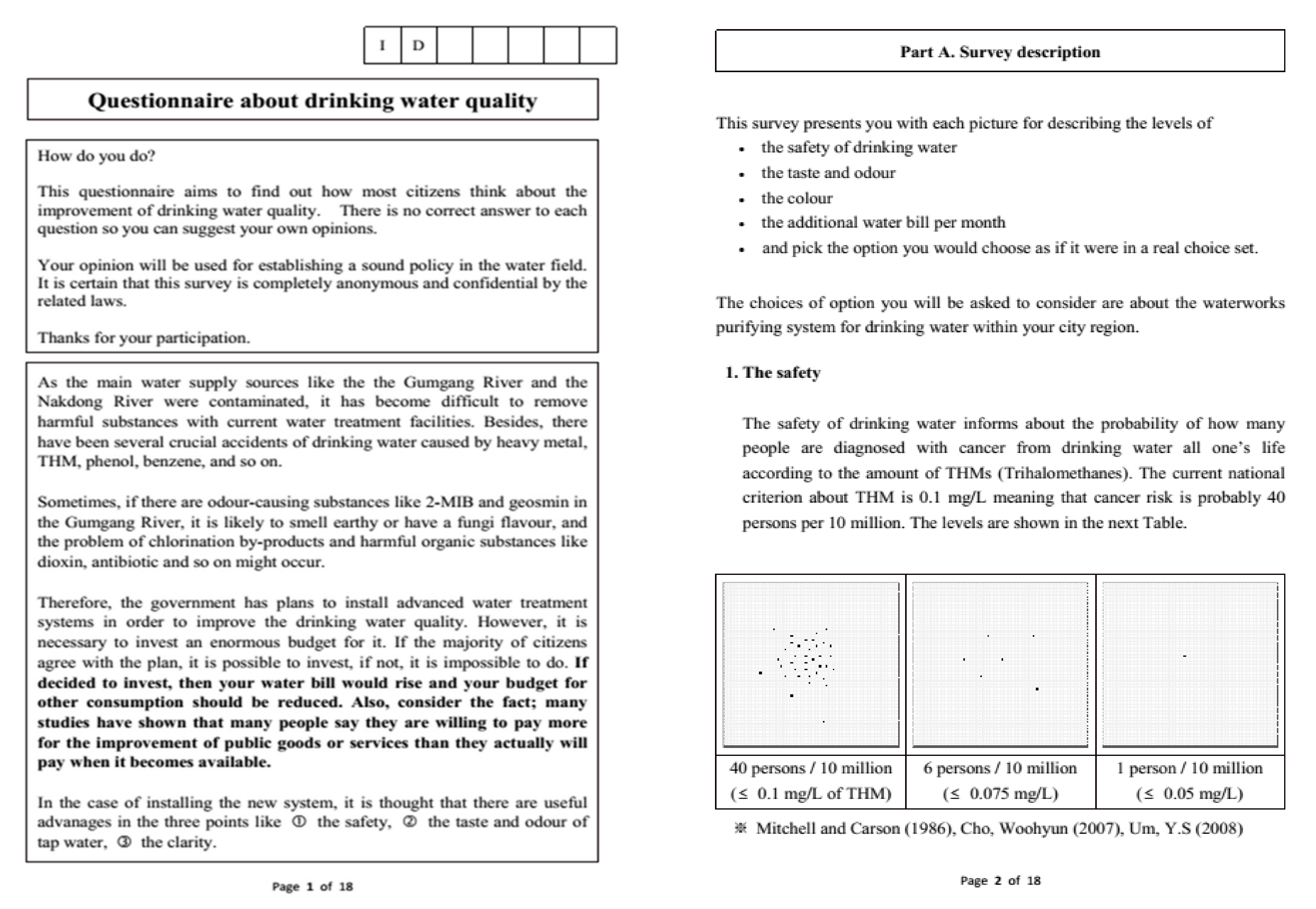
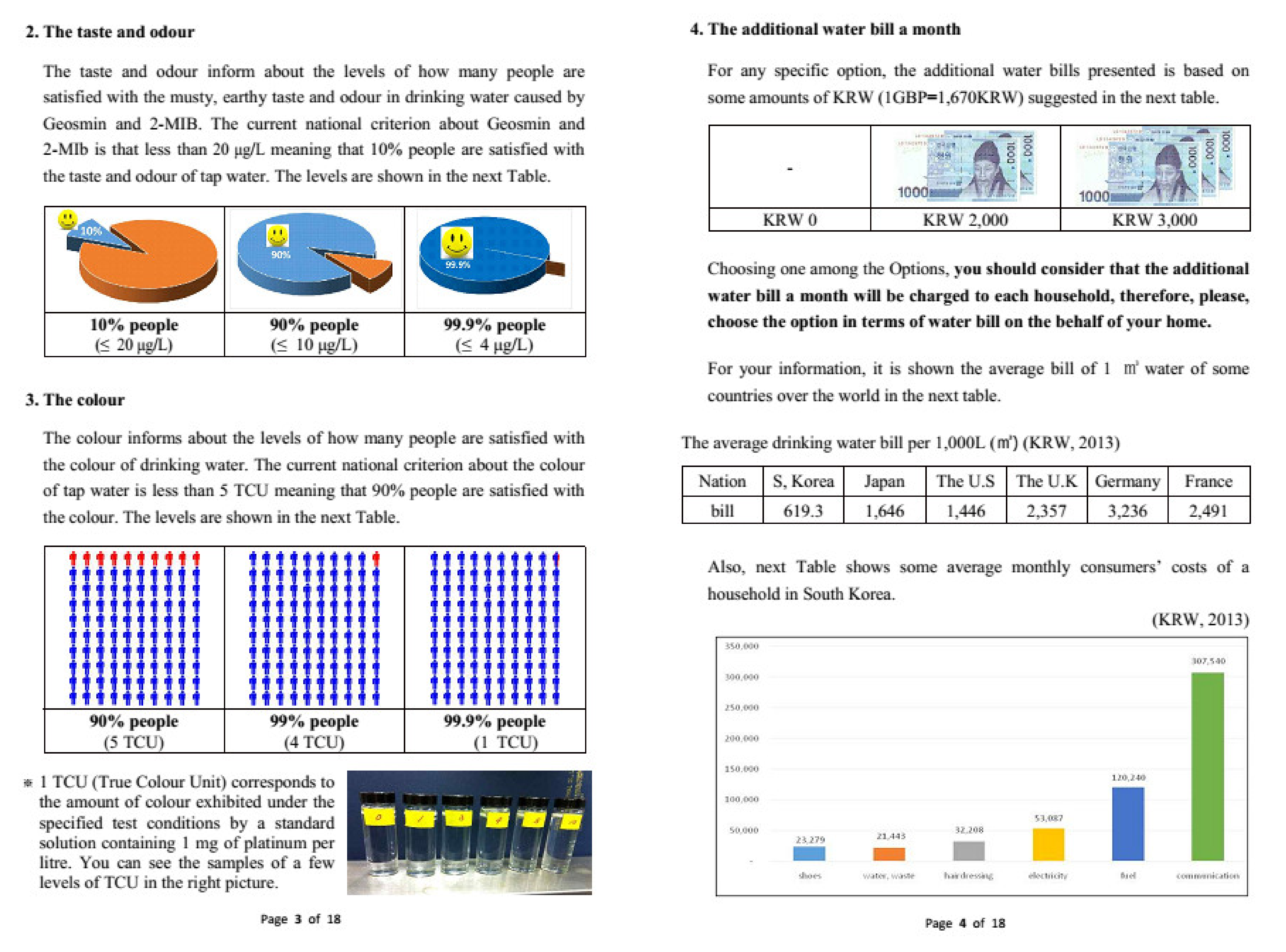
Before designing the choice sets, a set of attributes found in the literature to affect the choice of drinking water was developed. The list of the four attributes (safety, taste, odor, color and price) and the levels chosen for the analysis are presented in the Appendix A of the survey) as they were communicated to the consumer. The attributes were also chosen based on a survey performed by the Ministry of Environment for South Korea [18] on the main reasons why Korean people are not satisfied with drinking water quality. Reference [19] remarks that one risk factor (among others) is that chlorine disinfection is unable to remove trihalomethanes as a high concentration of trihalomethanes is related to cancer risk. The authors in [19] analyzed the relationship between the three types of treatment systems and the levels of trihalomethanes and found that status quo (of 0.1 mg/L) is associated with a cancer risk of 40 people per 10 million, whereas GAC and GAC + Ozone are associated with a risk of six and one per ten million, respectively. In this analysis, cancer risk is used for depicting the three levels of the safety attribute. Pollution (particularly in the form of blue–green algae) gives rise to unpleasant taste and odor in water. The proposed water treatment can influence this, and thus improve water taste and odor. References [19,20,21] demonstrate that moving from the status quo to GAC reduces pollution and increases satisfaction with water from 10% to 90%; moving from GAC to GAC + Ozone increases satisfaction to 99.9%.

The color of drinking water is linked to the concept of a true color unit (TCU). One TCU corresponds to the amount of color exhibited under the specified test conditions by a standard solution containing one milligram of platinum per liter. The current standard for the color of drinking water in South Korea is five TCU. Reference [10] reports that 7% of people complained about the color of drinking water in South Korea. Thus, it could be conservatively assumed that 10% of people were likely unsatisfied with the color of drinking water. It is also reported that GAC can reduce the color of drinking water to less than four TCU and GAC + Ozone can usually remove the color of drinking water to less than three TCU. References [22,23] reported that the 3 TCU level of drinking water color is the human detection limit. Therefore, it is assumed that the GAC + Ozone is linked to a cautious satisfaction level of 99.9%. In the case of the level of four TCU, it was assumed that 99% of people would be satisfied with the color because its level is very close to the human detection limit.

There have been no studies measuring the benefit of improving drinking water quality using choice experiments in South Korea, so there are no indicative prices about the benefits from improved attributes of drinking water quality; however, there are some contingent valuation studies calculating the WTP for improvements in drinking water quality mentioned above references [2,12,13,14]. This study borrows estimates for the levels of the price attribute from these. Accordingly, this study sets six levels of additional fees for the monthly water bill: 0 (Status Quo), USD 0.45 (KRW 500), USD 0.89 (KRW 1000), USD 1.79 (KRW 2000), USD 2.68 (KRW 3000) and USD 3.57 (KRW 4000).

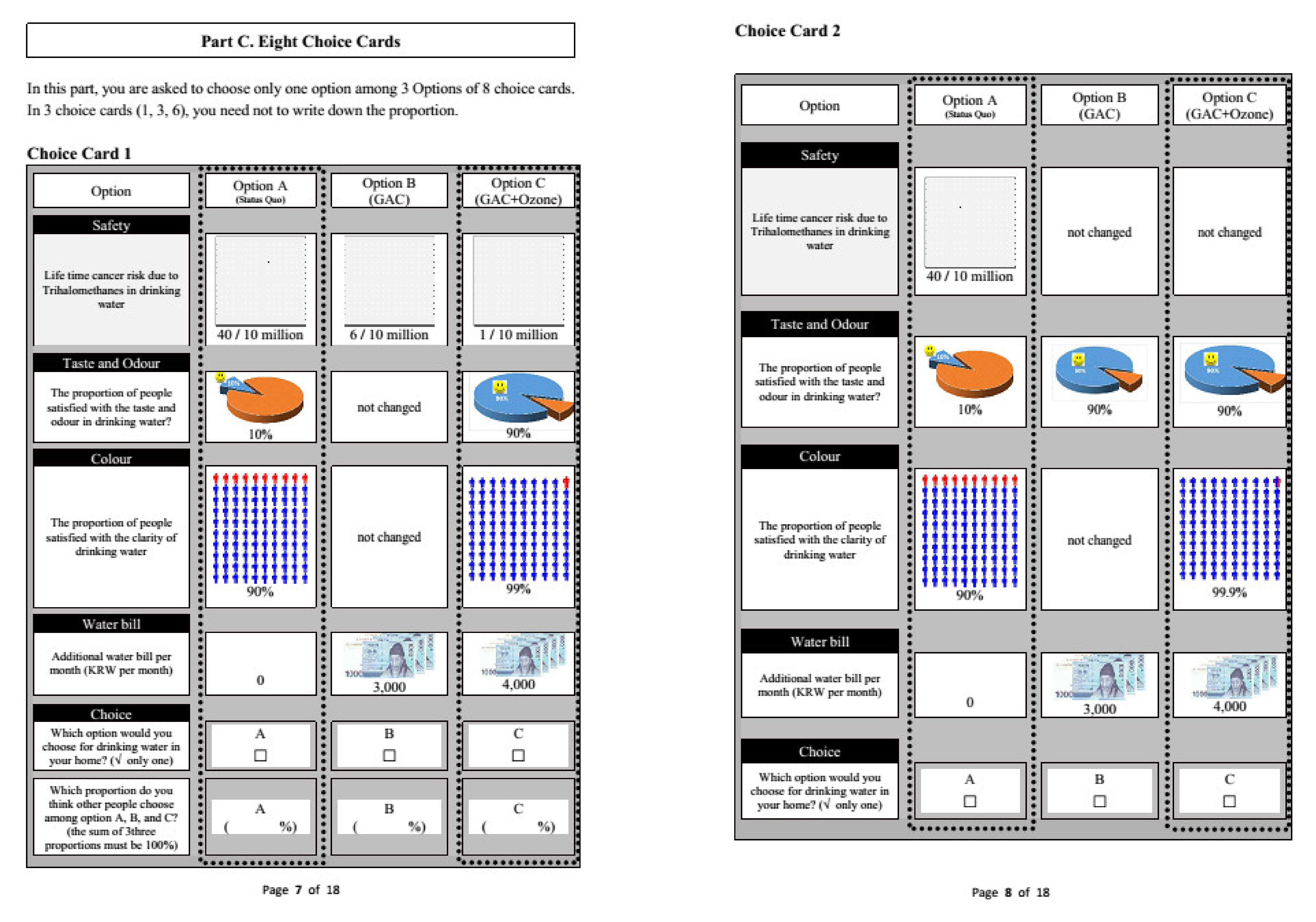
In this research, three options (status quo, GAC, GAC + Ozone) and four attributes (safety, taste and odor, color, and cost) are considered. Three attributes have three levels and cost has six levels. Therefore, the complete factorial design will be 162 ($3^3\times 6^1$). Obviously, it is impossible to confront the consumer with all these alternatives; therefore, a subset was chosen using a D-optimal design, the most prevalent approach for measuring the efficiency of experimental design [24]. The final design consists of 32 choice sets per product using the main effects design strategy. The questionnaire (Appendix A) presents 2 examples of a choice card/task implemented into the survey. As is often done in the literature, this study blocked the experiment into four sets of eight choices for each product such that the pairwise correlations among attribute levels are balanced, improving the estimation of the variance-covariance matrix. This study further used a between-subject design such that consumers were randomly assigned to one of the four treatments. Therefore, the respondents had to perform only 8 randomly chosen choice tasks in the survey, which is a number typically used [25,26]. Each respondent received a set of instructions for completing the survey and the choice task together with background information about the project and a detailed description of the attributes. Two different methods against hypothetical bias were employed as will be described below. A rich set of socio-economic characteristics were elicited together with the choice tasks in the survey and will be described in more detail in the data section.

2.2. Hypothetical Bias

It is often the case that stated preference studies demonstrate significant differences between stated versus real values. The difference between the two is called hypothetical bias [4,7]. As hypothetical bias is the strongest criticism brought to stated preferences techniques, the present choice experiment contains two different methods to reduce hypothetical bias as described in the introduction. The two methods were implemented using three different treatments: one where both cheap talk and honesty priming were used together, one where only cheap talk was used and one where only honesty priming was used. Consumers were randomly assigned to one of four blocks each corresponding to different treatments: block 1 corresponded to the use of both cheap talk and honesty priming, block 2 corresponded to the use of cheap talk only, block three corresponded to the use of honesty priming only and block four contained no treatment (for reference).

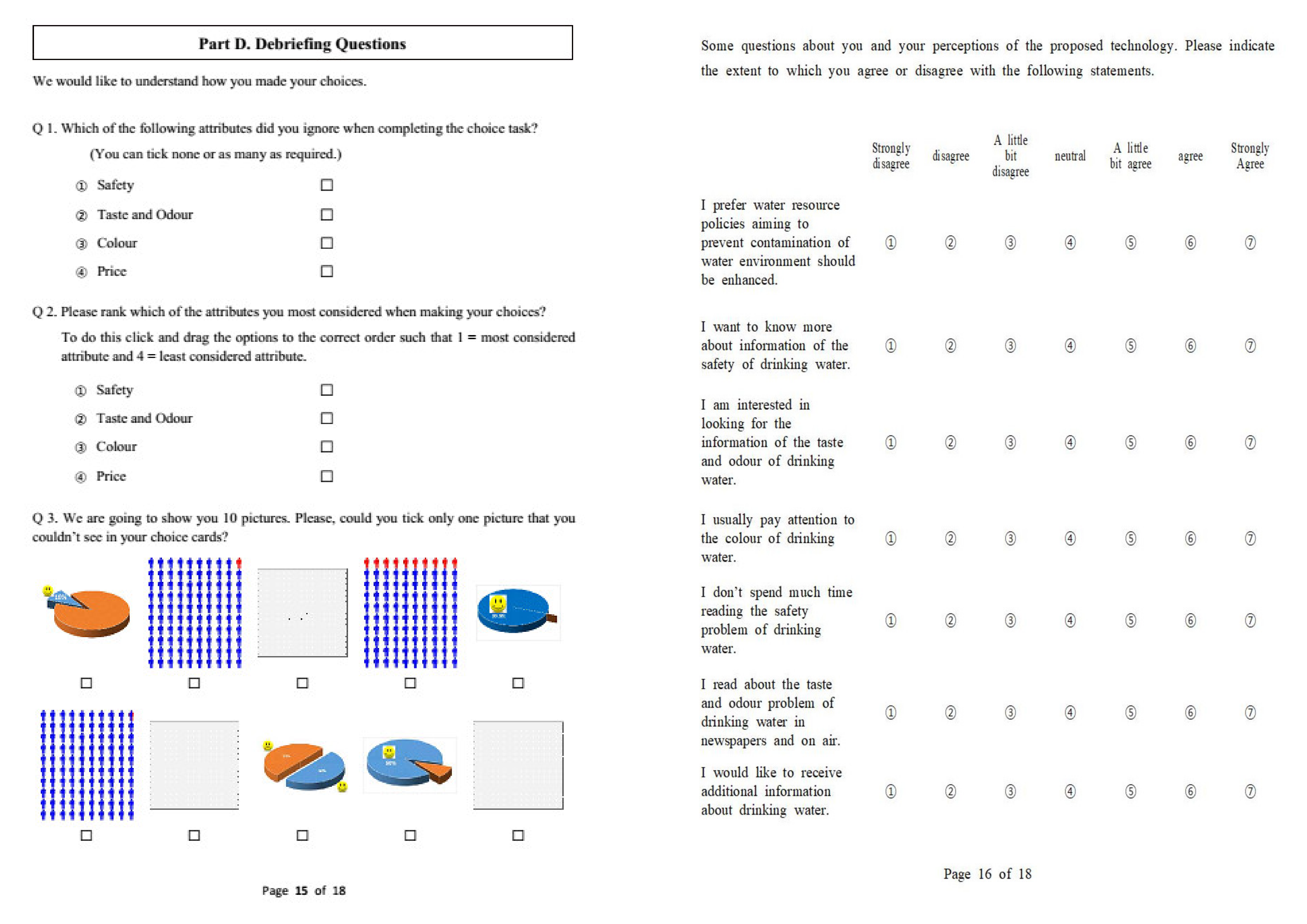
In total, 573 questionnaires were collected with 68 cases in which the respondents replied incorrectly to the debriefing question. Debriefing questions asked respondents to choose the pictures that they cannot see among the ten pictures on the choice cards. If respondents chose pictures that were on the choice cards, they were deemed to not be concentrating enough on the choice experiment and were eliminated from the sample. A further 98 cases were excluded because they chose the same alternatives in the eight choice cards and therefore it is deemed that sufficient attention may not have been given. Another case was excluded because it was an outlier with respect to the average monthly water bill: KRW 150,000 compared to the sample average of KRW 11,570. Therefore, 406 responses were used in the further analysis. This number of observations should be approximatively representative for the South Korean population. According to reference [27], Equation (1) on page 43 defines the sample size $\mathrm{n}=\underset{\mathrm{m}}{\max }{\mathrm{z}}^2\left(\frac{1}{\mathrm{m}}\right)\left(1-\frac{1}{\mathrm{m}}\right)/{\mathrm{d}}^2$ where m = nr of categories, (choices) = 3 in this study, d = allowed sampling error of 0.05, z = upper ($\mathsf{\alpha }/2\mathrm{m})\times 100\mathrm{th} \mathrm{percentile}$ of the standard normal distribution can be found in the tables for α = 0.05 and Φ(z) = 0.99 being equal to 2.3. Therefore, $\mathrm{n}=\frac{{2.3}^2\left(\frac{1}{3}\right)\left(1-\frac{1}{3}\right)}{{0.05}^2}\approx 470$.

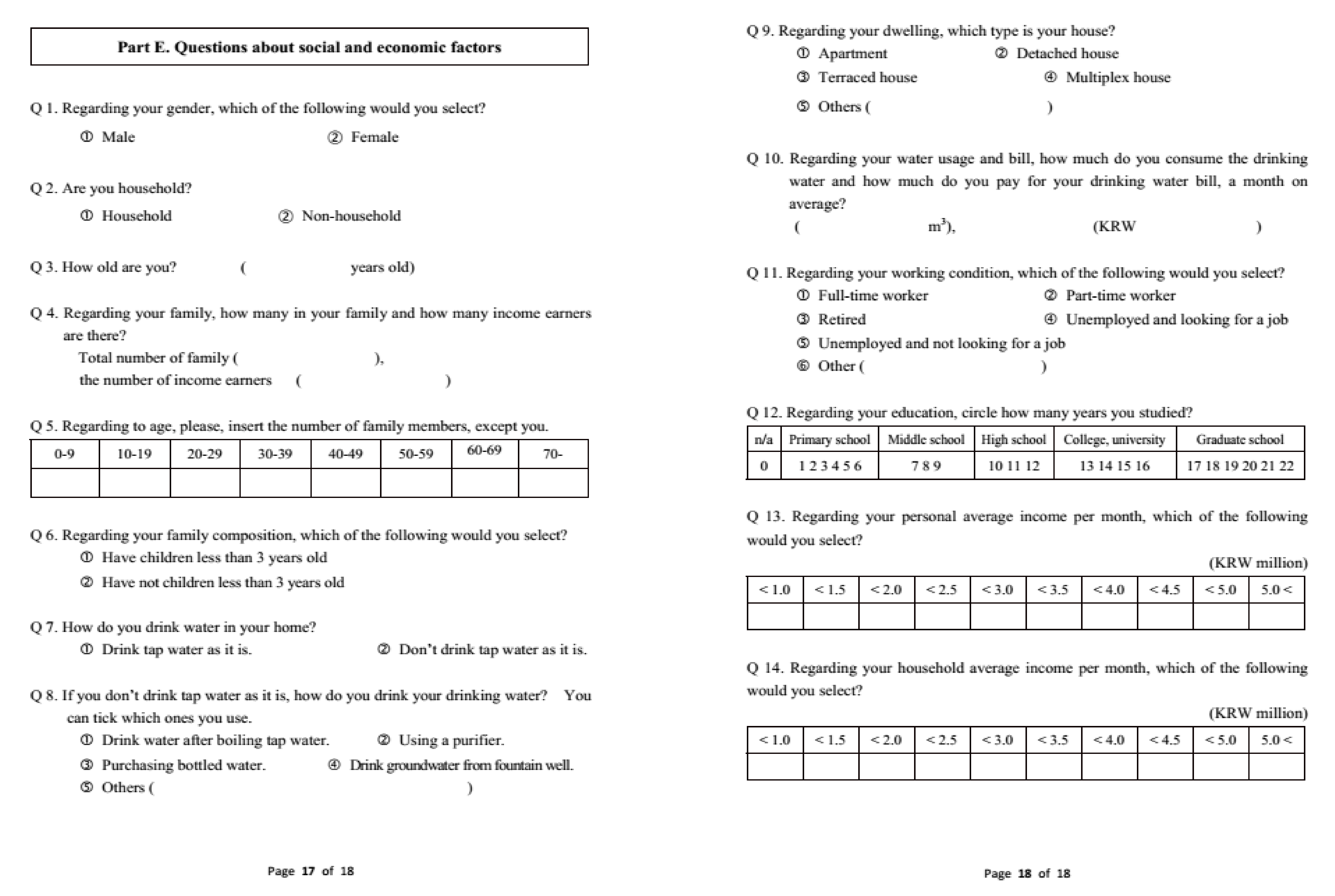
The survey consisted of five parts. Part (A) described the hypothetical scenario, the choice experiment, the attributes and their levels and gave an example of a choice card with explanations of the options available. Part (B) introduced the hypothetical bias treatments. Part (C) performed the choice experiment with the 8 choice cards presented to the respondents. Part (D) included three types of debriefing questions and one scale consisting of seven questions related to attitudes towards improvement of drinking water quality. The answers were ranked on a Likert type scale from 1 (Strongly Disagree) to 7 (Strongly Agree). The first type of debriefing questions asked the respondents about which attributes they might have ignored while making their choices. The second type of debriefing questions asked the respondents to rank the attributes according to their importance. The third type of debriefing questions aimed at determining the validity of the choices as described above. A homogeneity test [28] showed that the homogeneity between the 68 respondents that answered the debriefing questions incorrectly and the rest of the sample could be rejected at 1% level of significance. Part (E) of the questionnaire included the usual questions about socio-economic characteristics and also questions regarding alternatives to tap water, monthly water consumption and water bills. The socio-economic characteristics were used in order to determine the representativeness of the sample. A list of all socio-economic characteristics can be found in Appendix C.

Demographic information demonstrates that the sample was in line with that of the population with respect to the proportion of male participants (0.518 compared with 0.515 in the population), age (40.4 compared with 41.0), household income (4.4 KRW million compared with 4.3) and water bill (11,820 KRV compared with 11,429); the sample was slightly better educated with an average of 14.7 years of schooling compared with 13.3 in the population. Further, the average family size is 3.46, which is larger than the average family size of the population, 2.51. The family size of the sample might cause a bias of underestimation because many empirical studies have reported that family size negatively influences the stated willingness to pay [29,30]. This might counteract the potential overestimation resulting from a better educated sample.

3. Methodology

The present study uses random parameter logit and latent class logit models in order to estimate the WTP of the respondent and ultimately the benefits of the advanced water treatment systems. Moreover, it estimates confidence intervals for the lower bound of the WTP using bootstrapping and simulations. It then performs a cost-benefit analysis in order to assess the relationship of these benefits to the costs and to determine the feasibility of the project. Rather than discussing these methodological elements at length, they will be only shortly described here and discussed more together with the empirical results.

3.1. Random Utility Framework

The response to the choice between the three constructed choice alternatives (labelled as Status Quo, GAC, and GAC + Ozone) is modelled in a random utility framework using random parameter logit (RPL). RPL models are performant and are designed to overcome the limitations of a standard logit model by allowing for random taste variation, unrestricted substitution patterns and correlation in unobserved factors [31]. RPL achieves this by allowing model parameters as well as constants to be random, by allowing multiple observations with persistent effects and by allowing a hierarchical structure for parameters. A simple form of the choice probability for alternative i in the case of RPL can be described as follows:

$${\mathrm{P}}_{\mathrm{n},\mathrm{t},{ß}_{\mathrm{n}}}\left(\mathrm{i}\right)=\frac{{\exp }^{ \left({\mathsf{\alpha }}_{\mathrm{n}}+{ß}_{\mathrm{n}}{\mathrm{x}}_{\mathrm{nti}}\right)}}{{{\displaystyle \sum }}_{\mathrm{j}\in {\mathrm{C}}_{\mathrm{nT}}}{\exp }^{\left({\mathsf{\alpha }}_{\mathrm{n}}+{ß}_{\mathrm{n}}{\mathrm{x}}_{\mathrm{ntj}}\right)}}$$

(1)

where ${ß}_{\mathrm{n}}$ include both random and non-random parameters specific to individual n and the constant ${\mathsf{\alpha }}_{\mathrm{n}}$ is also allowed to be random (t = 1, …, T is the choice situation when the individual is faced with multiple choice situations), C_n is the choice set for individual n and ${\mathrm{x}}_{\mathrm{nti}}$ is a vector of observable independent variables that includes attributes of the alternatives, and socio-economic characteristics of the respondent. In order to estimate the coefficients of the RPL, it is necessary to maximize the likelihood ${\mathrm{P}}_{\mathrm{n},\mathrm{t},{ß}_{\mathrm{n}}}$ from Equation (1). To estimate the coefficient for representing a sample, a log-likelihood function is estimated through simulated methods, because (1) does not have a closed form.

3.2. Latent Class Model (LCM)

The latent class model is a semi-parametric extension of the multinomial logit model which allows the investigation of heterogeneity on a class (segment) level and relaxes the assumptions regarding the parameter distribution across individuals [32]. This approach has individuals endogenously grouped into classes of homogenous preferences [33,34] and estimates their probability of membership to their designated class depending on their socio-economic characteristics [35].

When examining the number of segments, the literature does not indicate a definite approach in selecting the correct number [28,33]. The standard specification tests used for maximum likelihood models appear to be inadequate [28] and therefore, other information criteria, such as the Akaike Information Criterion (AIC) and the Bayesian Information Criterion (BIC), are suggested as well as the judgement of the researcher on the interpretation of the findings [33]. In the present analysis, the models with the lowest BIC were selected.

3.3. Attribute Non-Attendance (ANA)

Reference [36] discusses that respondents may not always use all attributes when making their decision in choosing an alternative; some may intentionally or not, be ignored. According to reference [37] respondents do not use all attributes when making their decision and if this information is not taken into account the estimate of their willingness to pay could be influenced. In the present study the parameters were set to zero if an attribute had a zero coefficient in LCM and therefore, in this way, this study allows the data to decide on the attributes that are not attended and are not imposing a specific non-attendance structure on the model ex ante.

One of the main aims of the present study is to quantify the individual’s willingness to pay (WTP) for each attribute within the choice set. The WTP is calculated as the ratio of each attribute’s coefficient over the monetary value coefficient [28,38,39] and is interpreted as a change in value associated with an increase of the attribute by one unit. This measure can then be used in order to estimate the levels of welfare associated with various products and their attribute combinations in order to decide which one is most valued by the consumer. In the case of RPL, simulation is used to calculate the ratio between the attribute coefficients and the price. One simulation method for the WTP is the Krinsky–Robb method. For this, the Choleski factors of the estimated coefficients are calculated.

3.4. Cost-Benefit Analysis (CBA)

A variety of methods exist for studying the feasibility of investments in public sectors such as public roads, airports and water/air quality. Among these methods, cost-benefit analysis has historically played the most prominent role. In the present study three discounted cash flow rules are used: net present value (NPV), internal rate of return (IRR), and B/C ratio (B/C), as shown in

Table 1. Decision rules for CBA (Cost-Benefit Analysis).

Net Present Value (NPV)	$\mathrm{NPV}={\displaystyle {\displaystyle \sum }_{\mathrm{t}=1}^{\mathrm{T}}}\frac{\mathrm{E}\left({\mathrm{NB}}_{\mathrm{t}}\right)}{{\left(1+\mathrm{r}\right)}^{\mathrm{t}}}-{\mathrm{I}}_0$ NBt = Bt − Ct (the flow of net benefits in time t period)
B/C ratio (B/C)	$\frac{\mathrm{B}}{\mathrm{C}} \mathrm{ratio}={{\displaystyle \sum }}_{\mathrm{t}-0}^{\mathrm{T}}\raisebox{1ex}{${\mathrm{B}}_{\mathrm{t}}$}\!\left/ \!\raisebox{-1ex}{${\left(1+\mathrm{r}\right)}^{\mathrm{t}}$}\right./{{\displaystyle \sum }}_{\mathrm{t}=0}^{\mathrm{T}}\raisebox{1ex}{${\mathrm{C}}_{\mathrm{t}}$}\!\left/ \!\raisebox{-1ex}{${\left(1+\mathrm{r}\right)}^{\mathrm{t}}$}\right.$
Internal Rate of Return (IRR)	${\displaystyle {\displaystyle \sum }_{\mathrm{t}=0}^{\mathrm{T}}}\frac{{\mathrm{B}}_{\mathrm{t}}}{{\left(1+\mathrm{IRR}\right)}^{\mathrm{t}}}={\displaystyle {\displaystyle \sum }_{\mathrm{t}=0}^{\mathrm{T}}}\frac{{\mathrm{C}}_{\mathrm{t}}}{{\left(1+\mathrm{IRR}\right)}^{\mathrm{t}}}$

Note: r—discount rate, T—life-cycle of the project, I₀—initial investment cost.

below.

To calculate the discounted cash flow, it is necessary to have information on the future costs (${\mathrm{C}}_{\mathrm{t}}$) and benefits (${\mathrm{B}}_{\mathrm{t}}$). Estimates of business incomes and costs over the project life are used as substitute variables in private business. If the NPV is greater than zero, then the project can be accepted. IRR is the discount rate that makes NPV equal to zero and evaluates the feasibility of a project by calculating the minimum required rate of return in terms of opportunity cost. If the IRR of a project is greater than the opportunity cost, the project can be accepted. Finally, the B/C ratio is the reaction of total discounted benefits to costs. To account for risk and uncertainty, various sensitivity analysis are performed in the present study. Different life cycles of the project, various discount rates and cost increase scenarios are considered in order to assess the robustness of the results.

4. Empirical Results

4.1. Benefits

As described in the methodology section, the data will be analyzed using random parameter logit and latent class attribute non-attendance models.

4.1.1. RPL

The empirical specification for the RPL model can be written as follows:

$${\mathrm{U}}_{\mathrm{j}}={\mathsf{\alpha }}_{\mathrm{j}}+{\mathsf{\beta }}_{\mathrm{jk}}{\mathrm{X}}_{\mathrm{jk}}+{\mathsf{\gamma }}_{\mathrm{jl}}{\mathrm{Z}}_{\mathrm{jl}}+({\mathsf{\theta }}_{\mathrm{m}}{\mathrm{D}}_{\mathrm{m}}){\mathrm{X}}_{\mathrm{p}}+{\mathsf{\epsilon }}_{\mathrm{j}}$$

(2)

where ${\mathrm{U}}_{\mathrm{j}}$ are the utilities derived from each alternative j = 1, …, 3; ${\mathsf{\alpha }}_{\mathrm{j}}$ are the alternative specific constants related to each alternative. The alternative-specific constant of the status quo is set to zero for normalization. ${\mathsf{\beta }}_{\mathrm{jk}}$ are the coefficients of the four attributes (safety, odor and taste, color and price) summarized in the vector X, where k = 1,…, 4; ${\mathsf{\gamma }}_{\mathrm{jl}}$ are the coefficients of the socio-economic characteristics summarized in the vector Z, where l = 1,…, L; ${\mathsf{\theta }}_{\mathrm{m}}$ is the coefficient of the hypothetical bias treatment summarized in the vector D, where m = 1,.., 3; ${\mathrm{X}}_{\mathrm{p}}$ is the price coefficient; ${\mathsf{\epsilon }}_{\mathrm{j}}$ is the error term. The index indicating the individual is skipped for simplicity.

Four issues related to the RPL estimations need to be mentioned: first, utility functions can use alternative specific constants (ASCs) to reflect the average effect on utility of all factors not included in the model. ASCs related to each alternative are reported. Second, when using RPL models, it is necessary to specify the distributions of the coefficients of the attributes. The analysis uses the normal distribution for safety, taste and odor and color and keeps the coefficient of the cost variable as a fixed parameter for convenience of simulation and interpretation of the results [40]. Third, when analyzing RPL models, it is important to look into the significance of the standard deviation of the random parameters. As discussed in the methodology section, RPL assumes that the representative utility has a parameter vector that has its own distribution, and estimates the mean parameters and their density by maximizing the probability function. By this, RPLs can provide an individual parameter for each respondent and can accommodate the assumption that each individual has a different preference. The number of initiations of the random draws is 1000 [41]. If the standard deviation is significantly different from zero, the random parameters have significant variation which means that the respondents have different marginal utilities for the attributes. Fourth, hypothetical bias dummies are included in two different ways: “RPL1” uses them as alternative specific constants, in which case ${\mathsf{\theta }}_{\mathrm{m}}{\mathrm{D}}_{\mathrm{m}}$ are not multiplied with ${\mathrm{X}}_{\mathrm{p}}$, and “RPL2” uses them as interaction terms with the price. The hypothetical bias dummies used are: ${\mathrm{D}}_{\mathrm{both}}$ represents block 1 which uses both cheap talk and honesty priming for reducing the hypothetical bias; ${\mathrm{D}}_{\mathrm{cheap}}$ stands for block 2 using cheap talk; and ${\mathrm{D}}_{\mathrm{honest}}$ for block 3 using the honesty priming task. Block 4 works as the base group, as all dummy variables are zero. If people have a hypothetical bias of overstatement and the treatments for mitigating hypothetical bias are effective, the coefficients of the dummy variables will be negative. If the coefficients of dummies are negative and significant, the size of the cost coefficient as a denominator will increase so the WTP will decrease and the hypothetical bias treatment can be considered to have been effective.

Table 2. Estimations of RPL (Random Parameter Logit) 1 and RPL 2.

Variable	RPL 1	RPL 2
x1 (safety; cancer risk)	−0.0563 (0.0000)	−0.0437 (0.0000)
S.D of coefficient of x1	0.0419 (0.0000)	0.0613 (0.0000)
x2 (taste and odor)	0.0089 (0.0000)	0.0087 (0.0000)
S.D of coefficient of x2	0.0219 (0.0000)	0.0220 (0.0000)
x3 (color)	0.0174 (0.2118)	0.0058 (0.6541)
S.D of coefficient of x3	0.1675 (0.0000)	0.1667 (0.0000)
x4 (cost/price)	−1.0791 (0.0000)	−0.6511 (0.0000)
Dboth x4	-	−0.2343 (0.0145)
Dcheap x4	-	−0.2730 (0.0027)
Dhonest x4	-	−0.6582 (0.0000)
ASC Of Ozone	−1.1352 (0.1927)	−2.2388 (0.0092)
Elderly	−0.6303 (0.0224)	−0.6712 (0.0111)
Bill	0.0385 (0.0185)	0.0397 (0.0096)
Environ	0.6553 (0.0000)	0.6113 (0.0000)
Fulltime		−0.4936 (0.0488)
Dboth	−2.1771 (0.0000)	−
Dcheap	−1.8695 (0.0000)	−
Dhonest	−2.5258 (0.0000)	−
ASC Of GAC	1.7204 (0.0053)	0.5395 (0.3684)
Elderly	−0.5236 (0.0075)	−0.4764 (0.0112)
Bill	0.0137 (0.2999)	0.0138 (0.2414)
Environ	0.2205 (0.0292)	0.2241 (0.0277)
Fulltime	−	−0.4086 (0.0273)
Dboth	−1.1580 (0.0000)	−
Dcheap	−2.2261 (0.0000)	−
Dhonest	−1.6462 (0.0000)	−
Sample size	406	406
Log Likelihood	−2655.96	−2692.9
AIC	5353.9	5425.8
BIC	5438.1	5487.9
Pseudo ${\mathrm{R}}_{\mathrm{adj}}^2$	0.2533	0.2430

Note: The values in the parentheses represent p-values, and S.D stands for standard deviation.

shows the estimation results of the RPL1 and RPL2 models. In RPL1, the coefficients of the three attributes (safety, taste and odor, cost) are significant at the 99% significance level but the coefficient of color is insignificant. This result implies that color is the attribute for which people’s average preference is near zero. As expected, the signs for safety and cost are negative (safety is measured by the number of people associated with cancer risk, therefore the lower the number the higher the safety), and the one of taste and odor is positive. The three coefficients of the standard deviations are significant at the 99% significance level suggesting that each respondent has a different preference with respect to the three attributes.

The ASCs of the socio-economic factors are chosen when their coefficients are significant at least in one option at the 95% significance level. As we use attribute-non attendance (ANA) and chose only the socio-economic factors that are significant at 95%, we do not need to perform a multivariate analysis to reduce the number of variables considered in the analysis. Those which are significant are: “elderly”, “bill” and “environ”. “Elderly” has a negative coefficient suggesting that respondents living with elderly people in the household prefer the status quo. The positive coefficients of “bill” and “environ” suggest that people that consume more water and have higher water bills and people that have a positive attitude towards environmental measures related to water quality prefer the advanced water treatment systems as compared to the status quo. The variable “environ” measures the sum of the scale values of the preference for water-environment friendly policy contained at the end of in part D of the survey. The coefficients of the three dummies of hypothetical bias treatments (${\mathrm{D}}_{\mathrm{both}}$, ${\mathrm{D}}_{\mathrm{cheap}}$, ${\mathrm{D}}_{\mathrm{honest}}$) are negative and significant at the 99% significance level in the two advanced options, suggesting that all treatments of hypothetical bias were successful in reducing hypothetical bias resulted from overestimation.

RPL2 introduces the hypothetical bias dummies as interactions with the price. The coefficients of the four attribute variables show the expected direction and are significant at the 99% significance level, but the one for color is insignificant, similar to RPL1. All three random parameters show significant coefficients for standard deviations at the 99% significance level, which implies that the three random parameters have significant variations. Again the coefficients of the interaction terms of the hypothetical bias treatments are negative and significant at the 99% significance level, which suggests that the hypothetical bias treatments reduce the willingness to pay for improvement of the attributes. Among them, the coefficient of ${\mathrm{D}}_{\mathrm{honest}}·\mathrm{x}4$ has the largest value suggesting that honesty priming has been most successful in reducing hypothetical bias. RPL2 uses four socio-economic factors: “elderly”, “fulltime”, “bill” and “environ”. The coefficient of “fulltime” is significant at the 95% significance level and negative suggesting those respondents with full-time jobs prefer the status quo. The coefficient of the water bill variable is significant at the 95% significance level and positive only for the GAC + Ozone option. This result suggests that people who consume more drinking water are likely to prefer this option. The results of the two random parameter logit models are similar but RPL1 shows lower log-likelihood AIC, BIC, and a higher pseudo ${\mathrm{R}}^2$ than the RPL2, suggesting a better fit.

4.1.2. LCM-ANA

As mentioned in the methodology section, the latent class models are estimated controlling for attributes that were not attended with the help of attribute non-attendance (ANA) estimation. ANA can be an issue in CE where consumers are faced with a large number of choices within a short period of time [38]. With the help of debriefing questions, the researcher elicits the attributes that were least attended by the respondents and seeks to identify how setting their coefficients to zero may influence the analysis. In response to the question “Which of the following attributes did you ignore when completing the choice task?” 32.8% of respondents said color, with all other attributes between 8.1% and 9.6%.

This result is expected because people cannot presumably detect the differences between 5 and 3 TCU, and this was also suggested by the RPL results. Around 10% of the respondents answered that they ignore taste and odor. It may seem surprising that some people (8.4%) in the sample report to have ignored water bills when making their choices; however, given that the water bill is only a small proportion of monthly income (0.21%), this may be understandable. Safety appears to be the least ignored attribute which is consistent with the RPL results.

Another question asked the respondents to rank the attributes according to their preference. Many respondents answered that they prefer safety first and taste and odor second; in total, 346 respondents choose safety as the first attribute and 277 taste and odor as the second attribute. In the case of color and water bill, respondents answered that they are the least preferred two attributes, with 204 respondents preferring water bill to color. Safety appears to be definitively the most and color the least appreciated attribute.

The present study does not impose a specific attribute non-attendance structure and estimates latent class models and then sets the attributes that are ignored there equal to zero in the LCM-ANA specification. For this, full attribute attendance (FAA) latent class models were estimated first. As discussed in the methodology section, BIC values are used for choosing the optimal number of classes. Goodness of fit values for models from 2 to 9 classes are presented in Appendix B, both for models using hypothetical bias (HB) treatments as ASCs and for using them as interaction terms with the price. As can be observed, the optimal number of classes for the model using HB as ASCs is five and three for the model using HB as interaction terms. After these number of classes the BIC-value starts rising.

Identifying the insignificant attributes in the FAA1 class models estimated without restriction, and then restricting these to zero gives the following model structure for ANA1:

$$\begin{gathered} {\mathrm{U}}_{\mathrm{ij}|1}={\mathsf{\alpha }}_{\mathrm{j}|1}+{\mathsf{\beta }}_{\mathrm{safe}|1}{\mathrm{X}}_{\mathrm{safe}}+{\mathsf{\beta }}_{\mathrm{t}\&\mathrm{o}|1}{\mathrm{X}}_{\mathrm{t}\&\mathrm{o}}+{\mathsf{\beta }}_{\mathrm{col}|1}{\mathrm{X}}_{\mathrm{col}}+{\mathsf{\beta }}_{\mathrm{p}|1}{\mathrm{X}}_{\mathrm{p}}+{\mathsf{\gamma }}_{\mathrm{lj}|1}{\mathrm{Z}}_{\mathrm{l}}+{\mathsf{\theta }}_{\mathrm{m}|1}·{\mathrm{D}}_{\mathrm{m}}+{\mathsf{\epsilon }}_{\mathrm{ij}|1} \\ {\mathrm{U}}_{\mathrm{ij}|2}={\mathsf{\alpha }}_{\mathrm{j}|2}+{\mathsf{\beta }}_{\mathrm{safe}|2}{\mathrm{X}}_{\mathrm{safe} }+0·{\mathrm{X}}_{\mathrm{t}\&\mathrm{o}}+0·{\mathrm{X}}_{\mathrm{col}}+{\mathsf{\beta }}_{\mathrm{p}|2}{\mathrm{X}}_{\mathrm{p}}+{\mathsf{\gamma }}_{\mathrm{lj}|2}{\mathrm{Z}}_{\mathrm{l}}+{\mathsf{\theta }}_{\mathrm{m}|2}·{\mathrm{D}}_{\mathrm{m}}+{\mathsf{\epsilon }}_{\mathrm{ij}|2} \\ {\mathrm{U}}_{\mathrm{ij}|3}={\mathsf{\alpha }}_{\mathrm{j}|3}+{\mathsf{\beta }}_{\mathrm{safe}|3}{\mathrm{X}}_{\mathrm{safe}}+0·{\mathrm{X}}_{\mathrm{t}\&\mathrm{o}}+0·{\mathrm{X}}_{\mathrm{col}}+{\mathsf{\beta }}_{\mathrm{p}|3}{\mathrm{X}}_{\mathrm{p}}+{\mathsf{\gamma }}_{\mathrm{lj}|3}{\mathrm{Z}}_{\mathrm{l}}+{\mathsf{\theta }}_{\mathrm{m}|3}·{\mathrm{D}}_{\mathrm{m}}+{\mathsf{\epsilon }}_{\mathrm{ij}|3} \\ {\mathrm{U}}_{\mathrm{ij}|4}={\mathsf{\alpha }}_{\mathrm{j}|4}+{\mathsf{\beta }}_{\mathrm{safe}|4}{\mathrm{X}}_{\mathrm{safe}}+{\mathsf{\beta }}_{\mathrm{t}\&\mathrm{o}|4}{\mathrm{X}}_{\mathrm{t}\&\mathrm{o}}+0·{\mathrm{X}}_{\mathrm{col}}+{\mathsf{\beta }}_{\mathrm{p}|4}{\mathrm{X}}_{\mathrm{p}}+{\mathsf{\gamma }}_{\mathrm{lj}|4}{\mathrm{Z}}_{\mathrm{l}}+{\mathsf{\theta }}_{\mathrm{m}|4}·{\mathrm{D}}_{\mathrm{m}}+{\mathsf{\epsilon }}_{\mathrm{ij}|4} \\ {\mathrm{U}}_{\mathrm{ij}|5}={\mathsf{\alpha }}_{\mathrm{j}|5}+{\mathsf{\beta }}_{\mathrm{safe}|5}{\mathrm{X}}_{\mathrm{safe}}+{\mathsf{\beta }}_{\mathrm{t}\&\mathrm{o}|5}{\mathrm{X}}_{\mathrm{t}\&\mathrm{o}}+0·{\mathrm{X}}_{\mathrm{col}}+{\mathsf{\beta }}_{\mathrm{p}|5}{\mathrm{X}}_{\mathrm{p}}+{\mathsf{\gamma }}_{\mathrm{lj}|5}{\mathrm{Z}}_{\mathrm{l}}+{\mathsf{\theta }}_{\mathrm{m}|5}·{\mathrm{D}}_{\mathrm{m}}+{\mathsf{\epsilon }}_{\mathrm{ij}|5} \end{gathered}$$

(3)

where 1–5 are the number of classes, “safe, t&o, col, p” are indexes for the four attributes, l is the index for the socio-economic characteristics Z, m is the index for the hypothetical bias treatments represented by the dummies D, and $\mathsf{\epsilon }$ is the error term. The index for the individual is skipped for simplicity. It can be observed that in FAA1, color was the attribute ignored in most classes, as expected.

Table 3. Estimation of the coefficients of the ANA1 (Attribute Non-Attendance) model.

Variable	Class 1	Class 2	Class 3	Class 4	Class 5
x1 (safety)	−0.0115 (0.1685)	−0.0787 (0.0000)	−0.0315 (0.0000)	−0.0992 (0.0000)	−0.0659 (0.0000)
x2 (t&o)	0.022 (0.0016)	0.0 (fixed)	0.0 (fixed)	0.0091 (0.0763)	0.0249 (0.0000)
x3 (color)	0.1635 (0.0001)	0.0000 (fixed)	0.0000 (fixed)	0.0000 (fixed)	0.0000 (fixed)
X4 (cost)	−0.4385 (0.0162)	−1.6890 (0.0000)	−1.85815 (0.0000)	−0.4291 (0.0084)	−1.2237 (0.0000)
of Ozone, one	3.9368 (0.4143)	−10.3007 (0.0001)	−18.6362 (0.2240)	1.6704 (0.5182)	−2.4698 (0.0445)
Elderly	−1.5635 (0.1843)	−0.8538 (0.1485)	−5.6905 (0.9938)	8.1582 (0.9840)	−0.1390 (0.7508)
Bill	−0.0546 (0.3322)	−0.1164 (0.0432)	0.3009 (0.0442)	0.1269 (0.0093)	0.0249 (0.2348)
Environ	0.0982 (0.8803)	2.6911 (0.0000)	2.4889 (0.2331)	0.0109 (0.9686)	0.7965 (0.0003)
Dboth	−3.6684 (0.0472)	−4.2468 (0.0000)	−8.6509 (0.9438)	−1.9746 (0.2125)	−1.6949 (0.0136)
Dcheap	4.3111 (0.9981)	−2.1275 (0.0303)	−8.3258 (0.9792)	−5.2732 (0.0014)	−1.0262 (0.1561)
Dhonest	5.2144 (0.9988)	−4.4826 (0.0000)	0.0695 (0.9661)	−4.9345 (0.0023)	−2.6401 (0.0000)
of GAC, one	4.5498 (0.3429)	−0.9715 (0.5377)	2.6276 (0.0002)	2.5140 (0.3604)	−0.6299 (0.6164)
Elderly	−0.4004 (0.7747)	−1.4895 (0.0001)	−0.5352 (0.0751)	8.0302 (0.9842)	−0.5649 (0.0825)
Bill	−0.0086 (0.8787)	−0.1341 (0.0018)	0.1134 (0.0000)	0.1071 (0.0359)	−0.0386 (0.1066)
Environ	−0.2475 (0.7083)	1.1416 (0.0000)	−0.2641 (0.0455)	−0.0863 (0.7796)	0.8243 (0.0003)
Dboth	−1.8130 (0.3076)	−3.5534 (0.0000)	−0.6633 (0.0817)	−1.7025 (0.2631)	−1.3913 (0.0233)
Dcheap	4.7046 (0.9979)	−2.2884 (0.0000)	−1.4024 (0.0000)	−5.6954 (0.0005)	−1.8048 (0.0091)
Dhonest	6.8215 (0.9984)	−3.1666 (0.0000)	0.2009 (0.6191)	−4.5187 (0.0051)	−3.1014 (0.0000)
Class probability	0.185 (0.0000)	0.167 (0.0000)	0.220 (0.0000)	0.181 (0.0000)	0.247 (0.0000)
Sample size: 406, Log−likelihood: −2439.1, AIC: 5054.2, BIC: 5406.7, Pseudo−R2: 0.3071

Note: The values in the parentheses represent p-values.

presents the results of the estimation.

Class 1 ignores the safety attribute as its coefficient is insignificant; otherwise, in all other estimations of classes, providing this attribute was deemed important, it was estimated to be statistically significantly with the expected sign. The sample size of Class 1 is estimated at 75 (75 = 406 × 0.185, where 0.185 is the class probability). Safety is less important in Class 3 compared to Class 2 as the coefficient s is only half as large. In Class 4 the taste and odor is significant only at 10% suggesting that members of this class care less about this attribute than for safety and costs. Class 5 is the largest, consisting of 25% of the sample. With respect to the socio-economic variables, the estimates are in line with those from the RPL specification, with corresponding intuition.

To summarize, the coefficient of the safety attribute is significant in all classes except Class 1. This result implies that about 80% of the respondents would want to pay to improve the safety attribute in drinking water quality. The respondents included in Classes 1, 4 and 5 (60% of respondents) have the WTP to improve the taste and odor attribute because the coefficient of this attribute is significant in their classes. The coefficient of the color attribute is significant only in Class 1 (18.5% of the respondents), while the coefficient of the cost/price is negative and significant in all classes. This reinforces the results obtained from RPL and from debriefing questions. The discussion for ANA2 follows a similar pattern and can be obtained from the authors upon request.

4.1.3. Willingness to Pay

In what follows, the WTPs will be presented and discussed per attribute. When applying ANA, the WTP of each class is weighted by the individual specific probabilities of class membership in order to compute individual WTPs. The mean and median values of the individual WTPs are then calculated.

Table 4. Estimation of the mean and median WTPs (Willingness To Pay).

	Mean WTP				Median WTP
Model	RPL 1	RPL 2	ANA 1	ANA 2	RPL 1	RPL 2	ANA 1	ANA 2
Safety	0.0523	0.0491	0.0666	0.0974	0.0510	0.0434	0.0468	0.0396
Taste and odor	0.0082	0.0146	0.0146	0.0217	0.0090	0.0100	0.0063	0.0177
Color	0.0171	0.0048	0.0690	0.0284	0.0017	0.0000	0.0000	0.0020

Note: Measured in KRW thousand.

presents these per attribute and model.

As shown in

Table 5. Benefits using the median WTPs of the ANA1 model.

KRW 1000	Safety	Taste and Odor	Color	Sum
Median of WTP (m)	0.04676	0.00630	0
GAC	change of attribute ($\Delta {\mathrm{x}}_{\mathrm{i}})$	34 (40 to 6)	80 (10 to 90)	9 (90 to 99)
	Benefit (m × $\Delta {\mathrm{x}}_{\mathrm{i}}$)	1.590	0.504	0	2.094
Ozone + GAC	change of attribute ($\Delta {\mathrm{x}}_{\mathrm{i}}$)	39 (40 to 1)	89.9 (10 to 99.9)	9.9 (90 to 99.9)
	Benefit (m × $\Delta {\mathrm{x}}_{\mathrm{i}}$)	1.824	0.567	0	2.391

, ANA2 has the largest mean WTPs of all three attributes. The largest mean and median WTPs are for the safety attribute and the lowest are for the color attribute, as expected. Interestingly, the mean WTPs for taste and odor are smaller than those for color in RPL1, ANA1 and ANA2; however, the median values are always the smallest for the color attribute. Median values are always smaller than mean values.

Confidence intervals for the median values have been constructed using simulation and bootstrapping. The exact way is explained in Appendix D. The results of both estimation methods can be used for sensitivity analysis. For example, the range obtained with the simulation can be chosen for the safety attribute and the range from bootstrapping can be used for taste and odor, as they provide lower WTPs for the two attributes, respectively.

4.1.4. Estimation of Benefits

Willingness to Pay per Household

The WTP per household can be calculated for each attribute and each alternative j, by multiplying the improvement of each attributes with the willingness to pay for a one unit improvement:

$$\begin{gathered} {\mathrm{WTP}}_{\mathrm{j},\mathrm{safe}}=\Delta {\mathrm{x}}_{\mathrm{j},\mathrm{safe}}\times {\mathrm{MWTP}}_{\mathrm{safe}} \\ {\mathrm{WTP}}_{\mathrm{j},\mathrm{T}\&\mathrm{O}}=\Delta {\mathrm{x}}_{\mathrm{j},\mathrm{T}\&\mathrm{O}}\times {\mathrm{MWTP}}_{\mathrm{T}\&\mathrm{O}} \\ {\mathrm{WTP}}_{\mathrm{j},\mathrm{colour}}=\Delta {\mathrm{x}}_{\mathrm{j},\mathrm{colour}}\times {\mathrm{MWTP}}_{\mathrm{colour}} \end{gathered}$$

(4)

Reference [42] states that while the mean WTP is the correct measure to use from the standpoint of economic efficiency, the median WTP is probably the more appropriate measure to facilitate a democratic decision-making process. Therefore, in this research, the median WTPs are used. Table 5 shows examples of the WTP calculations per household for the two advanced treatment systems using the median WTP values of the ANA1 model as this provides the most conservative estimates.

Table 6. Benefits from the four models.

KRW	RPL 1	RPL 2	ANA 1	ANA 2
GAC	Mean	3.206	3.270	4.056	5.370
	Median	2.467	2.274	2.094	2.781
Ozone + GAC	Mean	3.633	3.703	4.596	6.035
	Median	2.813	2.589	2.391	3.156

shows the comparison of the benefits from the WTP estimates from the four different models.

As shown in Table 6, all benefits using the median WTPs are lower than those obtained for the mean WTPs. The median WTPs of the ANA1 model are always lower than for the other models. Therefore, the ANA1 model can be used as a lower bound. Furthermore, the benefits of all models can be used for sensitivity analysis.

Total Benefits

In order to estimate the total benefit of improving drinking water quality, it is necessary to know the population and the number of households served by the waterworks. In 2009, the number of people served by the waterworks was reported as 511,451 [43]. Unfortunately, there are no recent numbers about the people served; however, given the fact that the population has constantly increased while the consumption per capita has remained relatively constant, it is reasonable to assume that 511,451 constitutes a lower bound for benefits estimation. The average family size per household is reported as 2.6 [44]. Therefore, the number of households served is estimated to be 196,712.

The total benefits are calculated by multiplying the number of households served by the waterworks (196,712) with the WTPs per household obtained in Table 6.

Table 7. Monthly and annual social Benefits.

	Monthly				Annual
KRW Million (USD Thousand)	RPL 1	RPL 2	ANA 1	ANA 2	RPL 1	RPL 2	ANA 1	ANA 2
GAC	485 (412)	447 (380)	412 (350)	547 (465)	5823 (5026)	5368 (4558)	4944 (4199)	6565 (5575)
Ozone + GAC	553 (470)	509 (433)	470 (399)	621 (527)	6744 (5724)	6111 (5190)	5643 (4793)	7451 (6327)

Note: USD 1 = KRW 1177.5, based on the exchange rate of 31 December 2015.

shows the monthly and annual benefits for the two alternatives (GAC and Ozone + GAC) from the four models. The numbers in parentheses are the benefits expressed in US Dollars.

The total annual benefits from the GAC method are estimated to be between USD 4199 and 5575 thousand (KRW 4944–6565 million), and the benefits from the Ozone plus GAC treatment are from USD 4793–6327 thousand (KRW 5643–7451 million) using the median WTPs of the four models.

4.1.5. Cost Estimation

Several stages are involved in launching a new water treatment system including investigating, designing, contracting, building, and then maintenance and operation. In South Korea, all waterworks are owned and operated by national or local governments. Therefore, projects on waterworks often follow a public process. The cost of designing a project must be used in the bidding process. Usually, the cost of designing is set as an upper bound of the contract process. Every bidder has to bid the lowest price possible for competition. Therefore, most bids by governments in South Korea usually succeed with a lower price than the designed cost proposed by the governments. Design requires a significant expenditure. Legal investigation of the feasibility for a public project is usually implemented in the stage of basic design. Usually, the bidder suggesting the lowest price wins the contract. The remaining phases are construction and operation. As a result, it is not necessary to actually spend costs for design drawing until the feasibility has been demonstrated. Therefore, a preliminary cost is used to investigate the feasibility in this research. The construction period was set to 4 years (48 months) based on the estimates from eight similar previous projects which installed the GAC + Ozone in South Korea (Ministry of Environment, Sejon, Korea, 2009.) All the projects were completed in less than five years.

Table 8. Cost flows for the two advanced water treatment systems.

System	Year 1	Year 2	Year 3	Year 4	Year 5	Year 6	…	Year 24
GAC	1605	3776	11,479	11,479	11,930	451	451	451
(USD)	(1369)	(3220)	(9790)	(9790)	(10,175)	(385)	(385)	(385)
Ozone	466	1096	3332	3332	3332	41	41	41
(USD)	(397)	(935)	(2842)	(2842)	(2842)	(35)	(35)	(35)

Note: The price unit is KRW million. The exchange rate is based on 31 December 2015.

shows the cost flows including several types of costs such as investigating, designing, construction, supervision, and operating and maintenance for the two advanced water treatment systems.

If the project service is set to 10 years, the operating period would be counted between year 5 and year 14. As a result, the benefit of improved drinking tap water can be calculated over the same period of the project service length because the drinking tap water treated by the newly installed ozone and (or) GAC systems will be supplied between the fifth year and the last year (i.e., 14th or 24th year). These types of assumptions for the period play important roles in sensitivity analysis.

4.1.6. Cost-Benefit Analysis (CBA)

The assumptions made for the CBA are summarized in

Table 9. Summary of basic assumptions for CBA.

Factor		Range
Business life (years)		10–20
Social discount rate (%/year)		1–10
Benefit	WTP of safety (KRW 1000)	0.0365, 0.0465–0.0468
	WTP of taste and odor (KRW 1000)	0.0063, 0.0060–0.0066
	Advantaged household	165,828–196,712
Construction period (years)		4–6
Construction cost (KRW per m3/day)		127,645–153,425

Note: The bold figures provide the upper bounds of the CBA values; B/C, NPV, IRR.

. In addition to these assumptions, the extent to which people will benefit from improved water quality is considered. Reference [45] investigated the proportion of people who will change their source of drinking water, for example, from bottled water, in-line filter, and spring to drinking tap water in South Korea. They report that 84.3% of their respondents answered positively to the question: “Will you drink tap water when the quality of drinking tap water is improved?” Thus, 15.7% of people answered that they would not change their behaviors regarding drinking tap water even if the quality of drinking tap water is improved. In this case, the respondents would have zero willingness to pay to improve the quality of drinking tap water. The number of people that have negative ASCs for the two alternatives is estimated which found that the highest percentage is 15.5% (63 people) in the case of ANA2. To mitigate the effect of this group who is unwilling to pay, 15.5% of people will be excluded from the calculation of the benefits.

Present Values of the Cash Flows

To implement CBA, it is necessary to establish the cash flows for the costs and benefits of improving the drinking water quality. Next, the three types of decision rules are calculated to test the feasibility.

Benefit Flow

Table 10. Social benefits of improving drinking tap water quality.

KRW Million (USD Thousand)	GAC	Ozone Plus GAC
Monthly Social Benefit	412 (350)	470 (399)
Annual Social Benefit	4943 (4198)	5644 (4793)

Note: USD 1 = KRW 1177.5, based on the exchange rate of 31 December 2015. 4943 = 412 × 12.

summarizes the total monthly benefit for the two methods for improving drinking water quality within the target area estimated using ANA1.

The total annual social benefit from the GAC method for improving drinking water quality is estimated as KRW 4943 million, and the annual social benefit from the ozone plus GAC treatment is KRW 5644 million, using the median WTPs.

Another factor to discuss is when and how much of the social benefit should be applied to the cash flows. In this research, the first supply year is the fifth year after starting construction of the advanced water treatment systems; however, after five years, the social benefits might be changed by any change in the real purchasing power of money. The survey was conducted in 2015 so the benefit is estimated on the basis of the price in 2015.

In the last row of

Table 11. Cash flows of the GAC and GAC plus ozone alternatives (summarizing cost and benefit flows).

	GAC		GAC Plus Ozone
	Net Value	Present Value	Net Value	Present Value
2015	−1605	−1605	−2071	−2071
2016	−3776	−3579	−4872	−4662
2017	−11,479	−10,313	−14,811	−13,563
2018	−11,479	−9776	−14,811	−12,979
2019	−6987	−5859	−9618	−8065
2020	4492	3605	5152	4134
…	…	…	…	…
2038	4492	1632	5152	1872
	50,022	15,788	51,706	13,067

Note: Values are in KRW million. USD 1 = KRW 1177.5, based on the exchange rate of 31 December 2015. The project starts to yield benefits just in the last year of construction (2019).

, the NPV of the GAC alternative is estimated as KRW 15,788 million (USD 13 million) and for the GAC plus ozone 13,067 million (USD 11 million). The three discount cash flow methods allow a more exact analysis of which alternative is more effective.

Table 12. Cost-benefit analysis of the two alternatives.

KRW Million	Present Cost	Present Benefit	NPV	B/C Ratio	IRR
GAC	40,556	56,344	15,788	1.389	8.97%
(USD thousand)	(34,589)	(48,055)	(13,465)
Ozone + GAC	51,269	64,336	13,067	1.255	7.46%
(USD thousand)	(43,726)	(54,871)	(11,145)

Note: USD 1 = KRW 1172.5, based on the exchange rate of 31 December 2015.

shows the results of CBA of the two alternatives when using the whole dataset to calculate the social benefits.

The NPVs of the two alternatives are larger than zero, but this is a necessary and not sufficient condition of investment. If a discount rate of 8.97% and 7.46% applies to the GAC and GAC plus ozone alternative respectively, then its NPV would be zero and the B/C ratio would be one. The B/C ratio is recommended as the best decision-making tool [46]; by this measure, GAC (1.389) is preferred to GAC plus ozone (1.225).

Sensitivity Analysis

There is risk and uncertainty in forecasting future figures. Four categories of scenarios will be used to address these risks and uncertainties. The first is related to the risk premium approach, which adds a premium to the chosen social discount rate of 4.5%. The second concerns business life, which drops from 20 years to 10. The third increases construction costs by 20%, which is the percentage from comparing the largest unit construction cost among previous projects with the unit cost of the standard. The last category contains several scenarios that manipulate the benefits.

Risk Premium Approach

At a social discount rate of 1%, the NPV (B/C ration) for the GAC and GAC + Ozone alternatives are 39,907 KRW million (1.855) and 40,254 (1.687) respectively; similarly, at social discount rates of 10% these figures are −2257 KRW million (0.933) and −7002 (0.838). It can be observed from

Table 13. Outline of the sensitivity analysis.

Scenario	B/C		NPV (KRW) (Unit: Million)		IRR (%)
	GAC	Ozone + GAC	GAC	Ozone + GAC	GAC	Ozone + GAC
Basic	1.389	1.255	15,788 (USD 13.5)	13,067 (USD 11.1)	8.97	7.46
Discount rate increases (4.5–>10%)	1.286	1.159	11,176 (USD 9.5)	7901 (USD 6.7)	8.97	7.46
Business life reduces (20–>10 years)	0.889	0.798	−4268 (USD −3.6)	−9937 (USD −8.5)	2.12	0.06
Benefits decline to zero	0.800	0.723	−8099 (USD −6.9)	−14,208 (USD −12.1)	0.23	−1.11
Benefits during 10 years	1.012	0.909	479 (USD 0.4)	−4493 (USD −3.87)	4.72	2.83
Benefit with lower bound WTPs	1.149	1.037	6053 (USD 5.2)	1886 (USD 1.6)	6.32	4.95
Exclusion of households without Benefits	1.126	1.014	5100 (USD 4.4)	730 (USD 0.6)	6.04	4.68
Cost increase (20%)	1.181	1.064	8630 (USD 7.4)	3852 (USD 3.3)	6.64	5.26
One year delay of construction	1.362	1.234	14,324 (USD 11.7)	11,666 (USD 10.0)	8.31	7.04

Note: USD 1 = KRW 1172.5, the exchange rate based on 31 December 2015.

that an NPV of zero is associated with a discount factor of 8.97% and 7.46%, respectively.

Reduction of Business Life

In the case of ozone treatment, business life is reported to be between 15 and 20 years, and the physical service life of the GAC treatment is reported to be between 40 and 50 years. Sensitivity analysis considers when the business lives of the two alternatives vary from 10 to 20 years. At a business life of ten years, both projects become infeasible with negative NPVs. A business life of 12 and 14 years, respectively, makes the GAC and GAC plus ozone alternative feasible (holding all other assumptions fixes).

Decrease in Benefits

Several situations are examined for decreases in benefits. The first case assumes the benefits decrease to zero over 20 years, using a method similar to straight-line depreciation in accounting. As a result, the total social benefits are reduced by KRW 260 million for the GAC alternative, and KRW 297 million for the ozone plus GAC alternative every year, so they will be zero at the end of the period. Under this assumption, both projects become unfeasible, with a NPV of −8099 KRW million and -14,208 for the GAC and GAC plus ozone alternatives, respectively.

The second case assumes no benefit after the twelfth year of operation. Following the logic derived from the changes in business life, the GAC project is still feasible (with an NPV of 479 KRW million) but the GAC plus ozone project now has a negative net contribution.

Third, the results with a lower estimate of the benefits are considered using the lower bound in the 95% confidence interval of simulating the median values of the WTPs of the ANA1 model. In this case, the annual social benefit of the GAC decreases by KRW 854 million (17.3%) and the ozone plus GAC model decreases by KRW 981 (20.5%). Under this scenario, both projects are still feasible with positive NPVs and IRRs of 6.32% and 4.95% for the GAC and GAC + Ozone alternatives, respectively. When using the lower bound in the 95% confidence interval of the bootstrapping method, similar results prevail, with IRRs of 8.74% and 7.24%.

Finally, the CBA is examined when some residents do not wish to pay to improve the quality of drinking tap water. As previously discussed, 15.5% (63) of people serviced by the waterworks can be excluded in measuring the social benefits because they have a negative sum of the coefficients of the ASC and socioeconomic variables for both alternatives. With this assumption, both projects are still feasible holding all other assumptions fixed; the projects have positive NPVs, and IRRs of 6.04% and 4.68% for the GAC and GAC plus ozone alternatives, respectively. It is important to note that in the present analysis the surveyed households appear to be willing to pay in order to improve the tap water quality and hence it is assumed that they will start drinking water from the tap more frequently once the treatments are implemented. Moreover, when asked explicitly in a different study if they will drink tap water when its quality will be improved, a vast majority of consumers (84.3%) answered that they would [44]. Additionally, when performing a sensitivity analysis excluding 15.5% of the sample from the benefits, i.e., the consumers that might not change their behavior out of cultural habit, the project remains feasible (Table 13, row 11). Hence, the cultural factor does not appear to be a big limiting factor in the present analysis.

Increase in Costs

The assumption made is that there is a 20% increase in unit construction costs applying the upper bound of previous cases in South Korea. In this scenario, both projects remain feasible with positive NPVs and IRRs of 6.64% and 5.26% for the GAC and GAC plus ozone alternatives, respectively. Assuming there is a one-year delay in construction, delaying the benefits, also results in the feasibility of both projects being maintained, holding all other assumptions fixed. Both the GAC and GAC plus ozone alternatives have positive NPVs and IRRs of 8.31% and 7.04%, respectively.

Summary of Sensitivity Analysis

Table 13 summarizes the various sensitivity analysis scenarios. Increasing the social discount factor to 10%, decreasing the useful life of the project, and significantly cutting the estimated benefits can make the alternative investments unfeasible; however, as outlined above, these are all extreme outliers. Further, where possible, benchmark assumptions have been conservative.

5. Conclusions

This study was triggered by the fact that many Koreans are dissatisfied with drinking water quality. Many rivers have been polluted due to the fast industrialization in South Korea. As a result, most waterworks at present have confronted problems like unpleasant taste and odor of drinking tap water. The Korean government has planned to improve water quality to resolve the issue. Installing advanced water treatment systems has been a primary solution. This research focuses on testing how far an investment in a chosen advanced water treatment system in the target are of Cheongju City is feasible.

The present study uses choice experiments in order to assess the benefits from installing two advanced water treatment systems in the target area and then performs an extensive cost-benefit analysis to assess the feasibility of the project under various scenarios. No other study has performed this type of analysis for South Korea, a developed country with a historically polluted water supply. The study employs two different methods to mitigate hypothetical bias (cheap talk and honesty priming) and finds both are effective in reducing it, with honesty priming being more successful than cheap talk. Honesty priming had the largest coefficient and was significant in most cases, hence appears to work best for the South Korean consumer as a method for dealing with hypothetical bias. This is considered an important contribution to the state of practice, as hypothetical bias is the strongest criticism brought to the elicitation of stated preferences and results obtained without this correction might be misleading and not suited for policy recommendations. The estimation of the benefit is done using random parameter logit models and attribute non-attendance latent class models. By this, it allows for random taste variation among the individuals and some attributes of drinking water are ignored. Moreover, it allows us to group individuals in latent classes and to determine which attributes are most valued by specific groups of respondents. The most important attribute to consumers was water safety, whereas color was not an issue for respondents; 50–60% of respondents are willing to pay in order to improve the taste and the odor of potable water. The average WTP for installing the granular activated carbon treatment is between USD 1.78 and 4.56 and for additionally installing an ozone purification system is USD 2.03–5.13 per month. These values are comparable with results obtained in previous studies and with the average spend for bottled water per month by South Koreans (Database of the Korean Statistical Information Service). For the cost-benefit analysis, median values have been used as more conservative values. Moreover, confidence intervals for the lower bound of these median values have been estimated using bootstrapping and simulations. This has not been done before in this context and is another important contribution to the methodological discourse rendering more robust WTP estimates.

Under the conservative assumptions of a construction period of five years, a social discount rate of 4.5% and a business life between 15–20 years, the feasibility of the project is given and the investments in both alternatives appear to be beneficial to the residents of Cheongju. The feasibility is maintained if the construction period is increased by one year, the social discount rate increases to 7%, a premium of 20% is added to the costs, and if the number of people benefitting from the improvement is reduced by 15.5%. If the business life falls below 12 years, the discount rate increases above 7.4%, the costs by more than 44% and the benefits gradually decrease to zero during the business life, thus the feasibility of the projects is rejected; however, as discussed, these situations are very unlikely to occur. Throughout the various sensitivity analyses, the granular activated carbon (GAC) model was the more robust treatment showing higher benefit/cost ratios, net present values and internal rate of returns. Therefore, if financial constraints shall exist, this alternative shall be preferred.

The present study has several limitations. Firstly, only a restricted number of attributes are considered. Further studies could consider additional attributes, such as for example “chlorine taste”, and might also consider interaction effects between these attributes. Benefits are just estimated based on the households serviced by the waterworks; however, restaurants and other commercial units that profit from water treatments could also be considered in order to provide a more comprehensive measure.

Most importantly, the analyses in this study focused on a short-term solution. Installing more advanced water treatment systems is dealing with the effects of pollution and not its causes. If these are not addressed, eventually the water quality would worsen to a point where it is not possible to treat it anymore. Improving raw water quality in the catchment and preventing water pollution in the basin should be wider policy prospects for the future. As studies have identified, livestock sewage is the main cause for water pollution in the target area and measures aiming at reducing this should be pursued [47]. Such measures could be: installing livestock sewage treatment facilities, building artificial swamps and detention ponds to deter the inflow of polluted water into the catchment, growing aquatic plants which can resolve pollutants in the waterways, and building detention facilities of sewage treatment plants. The Committee of Managing the Geuem River Basin has developed additional projects for preventing pollutants to enter the basin among which are the maintenance of the drainage systems, provision of eco-friendly agricultural materials, building buffers and afforestation [48]. Such measures need to become the priority of policy so the quality of drinking water shall not further deteriorate and clean potable water can be supplied to South Korean citizens in a sustainable way. The feasibility of such projects shall constitute the scope of future research and should be used as one criteria among others in a decision process involving several stakeholders.

References

- UN World Water Development Report 2017. Available online: http://www.unwater.org/publications/world-water-development-report-2017/ (accessed on 15 January 2018).
- Um, M.-J.; Kwak, S.-J.; Kim, T.-Y. Estimating Willingness to Pay for Improved Drinking Water Quality Using Averting Behavior Method with Perception Measure. Environ. Resour. Econ. 2002, 21, 285–300. [Google Scholar] [CrossRef]
- Ministry of Environment. Study for Satisfaction of Tap Water in Korea, 2012; Ministry of Environment: Sejong, Korea, 2013. (In Korean)
- Cummings, R.G.; Taylor, L.O. Unbiased Value Estimates for Environmental Goods: A Cheap Talk Design for the Contingent Valuation Method. Am. Econ. Rev. 1999, 89, 649–665. [Google Scholar] [CrossRef]
- Gschwandtner, A.; Burton, M. Comparing treatments to reduce hypothetical bias in choice experiments regarding organic food. Eur. Rev. Agric. Econ. 2020, 47, 1302–1337. [Google Scholar] [CrossRef]
- Loomis, J.B. Strategies for Overcoming Hypothetical Bias in Stated Preference Surveys. J. Agric. Resour. Econ. 2014, 39, 34–46. [Google Scholar]
- Penn, J.; Hu, W. Cheap talk efficacy under potential and actual Hypothetical Bias: A meta-analysis. J. Environ. Econ. Manag. 2019, 96, 22–35. [Google Scholar] [CrossRef]
- De-Magistris, T.; Gracia, A.; Nayga, R.M. On the Use of Honesty Priming Tasks to Mitigate Hypothetical Bias in Choice Experiments. Am. J. Agric. Econ. 2013, 95, 1136–1154. [Google Scholar] [CrossRef]
- McManus, R.; Haddock-Fraser, J.; Rands, P. A methodology to understand student choice of higher education institutions: The case of the United Kingdom. J. High. Educ. Policy Manag. 2017, 39, 1–16. [Google Scholar] [CrossRef]
- Kwak, S.J. Contingent Valuation of Improving Safety of Tap Water Quality in Seoul. Korea Spat. Plan. Rev. 1994, 21, 23–40. (In Korean) [Google Scholar]
- Yoo, S.H.; Yang, H.J. Application of Sample Selection Model to Double-Bounded Dichoto-mous Choice Contingent Valuation Studies. Environ. Resour. Econ. 2001, 20, 147–163. [Google Scholar] [CrossRef]
- Park, D.; Ko, Y.; Kwon, O.; Kim, W. Building of Evaluation System of Water Resources and Water Related Technology; Ministry of Science and Technology: Gwacheon, Korea, 2007. (In Korean)
- Kwak, S.-Y.; Yoo, S.-H.; Kim, C.S. Measuring the Willingness to Pay for Tap Water Quality Improvements: Results of a Contingent Valuation Survey in Pusan. Water 2013, 5, 1638–1652. [Google Scholar] [CrossRef] [Green Version]
- Na, J. Cost-Benefit Analysis of the Introduction of Advanced Water Treatment Process: Focused on the case of ’K-Water B Water Treatment Plant; Seoul National University: Seoul, Korea, 2013. (In Korean) [Google Scholar]
- Mitchell, R.C.; Carson, R.T. Valuing drinking water risk reductions using the contingent valuation method: A methodological study of risks from THM and Giardia. In Resources for the Future; EPA: Washington, DC, USA, 1986. [Google Scholar]
- List, J.A.; Gallet, C.A. What Experimental Protocol Influence Disparities Between Actual and Hypothetical Stated Values? Environ. Resour. Econ. 2001, 20, 241–254. [Google Scholar] [CrossRef]
- Penn, J.M.; Hu, W. Understanding Hypothetical Bias: An Enhanced Meta-Analysis. Am. J. Agric. Econ. 2018, 100, 1186–1206. [Google Scholar] [CrossRef]
- Ministry of Environment. Statistics of Waterworks, 2013; Ministry of Environment: Sejong, Korea, 2014. (In Korean)
- Cho, W. Advanced Water Treatment Processes to Remove Taste and Odour of Raw Water in the Han River; University of Seoul: Seoul, Korea, 2007. [Google Scholar]
- Pirbazari, M.; Ravindran, V.; Badriyh, B.N.; Craig, S.; McGuire, M.J. GAC Absorber Design Protocol for the Removal of off-flavours. Water Resour. 1993, 27, 1153–1166. [Google Scholar]
- Ho, L.; Croue, J.-P.; Newcombe, G. The effect of water quality and NOM character on the ozonation of MIB and geosmin. Water Sci. Technol. 2004, 49, 249–255. [Google Scholar] [CrossRef] [PubMed]
- Choi, J.; Park, T. Estimation of social discount rate for analysing the economic feasibility of public projects. J. Soc. Sci. South Korea 2015, 41, 145–167. [Google Scholar]
- Bean, E.L. Progress Report on Water Quality Criteria. J. Am. Water Work. Assoc. 1962, 54, 1313–1331. [Google Scholar] [CrossRef]
- Ferrini, S.; Scarpa, R. Designs with a priori information for nonmarket valuation with choice experiments: A Monte Carlo study. J. Environ. Econ. Manag. 2007, 53, 342–363. [Google Scholar] [CrossRef]
- Burton, M.; Rogers, A.A.; Richert, C. Community acceptance of biodiversity offsets: Evidence from a choice experiment. Aust. J. Agric. Resour. Econ. 2016, 61, 95–114. [Google Scholar] [CrossRef] [Green Version]
- Balcombe, K.; Fraser, I.; Lowe, B.; De Souza-Monteiro, D.M. Information Customization and Food Choice. Am. J. Agric. Econ. 2015, 98, 54–73. [Google Scholar] [CrossRef]
- Thompson, S.K. Sample Size for Estimating Multinomial Proportions. Am. Stat. 1987, 41, 42–46. [Google Scholar]
- Bera, A.K.; Greene, W.H. Econometric Analysis. J. Am. Stat. Assoc. 1994, 89, 1567. [Google Scholar] [CrossRef]
- Ahlheim, M.; Schneider, F. Considering Household Size in Contingent Valuation Studies. Environmental Economics. 2013, 3, 112–123. [Google Scholar]
- Chambers, C.M.; Chambers, P.E.; Whitehead, J.C. Contingent Valuation of Quasi-Public Goods: Validity, Reliability, and Application to Valuing a Historic Site. Public Financ. Rev. 1998, 26, 137–154. [Google Scholar] [CrossRef]
- Train, K.; Weeks, M. Discrete choice models in preference space and willing-to-pay space. In Applications of Simulation Methods in Environmental and Resource Economics, Chapter 1; Scarpa, R., Alberini, A., Eds.; Springer: Dordrecht, The Netherlands, 2005; pp. 1–16. [Google Scholar]
- Greene, W.H.; Hensher, D.A. Modeling Ordered Choices; Cambridge University Press (CUP): Cambridge, UK, 2009. [Google Scholar]
- Scarpa, R.; Thiene, M. Destination Choice Models for Rock Climbing in the Northeastern Alps: A Latent-Class Approach Based on Intensity of Preferences. Land Econ. 2005, 81, 426–444. [Google Scholar] [CrossRef]
- Hammitt, J.K.; Herrera-Araujo, D. Peeling back the onion: Using latent class analysis to uncover heterogeneous responses to stated preference surveys. J. Environ. Econ. Manag. 2018, 87, 165–189. [Google Scholar] [CrossRef] [Green Version]
- Kikulwe, E.M.; Birol, E.; Wesseler, J.; Falck-Zepeda, J. A latent class approach to investigating demand for genetically modified banana in Uganda. Agric. Econ. 2011, 42, 547–560. [Google Scholar] [CrossRef]
- Hensher, D.A.; Shore, N.; Train, K. Households’ Willingness to Pay for Water Service Attributes. Environ. Resour. Econ. 2005, 32, 509–531. [Google Scholar] [CrossRef]
- Mariel, P.; Hoyos, D.; Meyerhoff, J. Stated or inferred attribute non-attendance? A simulation approach. Econ. Agrar. y Recur. Nat. 2013, 13, 51–67. [Google Scholar] [CrossRef] [Green Version]
- Loureiro, M.L.; Umberger, W.J. A choice experiment model for beef: What US consumer responses tell us about relative preferences for food safety, country-of-origin labeling and traceability. Food Policy 2007, 32, 496–514. [Google Scholar] [CrossRef]
- Kerr, G.N.; Sharp, B.M. Efficient design for willingness to pay in choice experiments: Evidence from the field. In Proceedings of the Paper presented at the New Zealand Agricultural and Resource Economics Society Conference, Nelson, New Zeeland, 27–28 August 2009. [Google Scholar]
- King, S.; Fraser, I.M.; O’Hanley, J.R. Benefits transfer and the aquatic environment: An investigation into the context of fish passage improvement. J. Environ. Manag. 2016, 183, 1079–1087. [Google Scholar] [CrossRef]
- Bhat, C. Quassi-Random Maximum Simulated Likelihood Estimation of the Mixed Multinomial Logit Model. Transp. Res. 2001, 35, 677–693. [Google Scholar] [CrossRef] [Green Version]
- Lockwood, M.; Loomis, J.; DeLacy, T. A Contingent Valuation Survey and Benefit-Cost Analysis of Forest Preservation in East Gippsland, Australia. J. Environ. Manag. 1993, 38, 233–243. [Google Scholar] [CrossRef]
- Ministry of Environment. Statistics of Waterworks, 2009; Ministry of Environment: Sejong, Korea, 2010. (In Korean)
- Cheongju City. Cheongju City Statistical Yearbook of 2014; Cheongju City: Cheongiu, Korea, 2015. (In Korean) [Google Scholar]
- Jo, Y.-M.; Kim, D.-W.; Hong, Y.-S. Strategies to Promote the Use of Tap Water for Drinking in Gyeonggi-Do; Geonggi Research Institute: Sejong, Korea, 2015. (In Korean) [Google Scholar]
- Pearce, D.W. Cost-Benefit Analysis; Springer Science and Business Media LLC: Berlin, Germany, 1983. [Google Scholar]
- Kim, J.W.; Jeong, S.A.; Kim, S.W.; Byeon, C.Y.; Lee, S.W. Master Plan for Managing Water Quality in Lake Daecheong; Korea-Water Institute: Daejeon, Korea, 2013. [Google Scholar]
- Committee of Managing the Geum River Basin. Project Plan for Supporting Residents in the Water Resource Management Area of Geum River Basin, 2017; Committee of Managing the Geum River Basin: Daejeon, Korea, 2016. (In Korean) [Google Scholar]
- Thiene, M.; Scarpa, R. Deriving and Testing Efficient Estimates of WTP Distributions in Destination Choice Models. Environ. Resour. Econ. 2009, 44, 379–395. [Google Scholar] [CrossRef]
- Train, K.; Weeks, M. Discrete Choice Models in Preference Space and Willingness-to-Pay Space. In The Economics of Non-Market Goods and Resources; Springer Science and Business Media LLC: Dordrecht, The Netherlands, 2005; pp. 1–16. [Google Scholar]