Exploring Wetland Dynamics in Large River Floodplain Systems with Unsupervised Machine Learning: A Case Study of the Dongting Lake, China

Abstract

Large river floodplain systems (LRFS) are among the most diverse and dynamic ecosystems. Accurately monitoring the dynamics of LRFS over long time series is fundamental and essential for their sustainable development. However, challenges remain because the spatial distribution of LRFS is never static due to inter- and intra-annual changes in environmental conditions. In this study, we developed and tested a methodological framework to re-construct the long-term wetland dynamics in Dongting Lake, China, utilizing an unsupervised machine-learning algorithm (UMLA) on the basis of MODIS (Moderate Resolution Imaging Spectroradiometer) EVI (Enhanced Vegetation Index) time series. Our results showed that the UMLA achieved comparable performance to the time-consuming satellite image segmentation method with a Kappa coefficient of agreement greater than 0.75 and an overall accuracy over 85%. With the re-constructed annual wetland distribution maps, we found that 31.35% of wet meadows, one of most important ecological assets in the region, disappeared at an average rate of c.a. 1660 ha year⁻¹ during the past two decades, which suggests that the Dongting Lake is losing its ecological function of providing wintering ground for migratory water birds, and remediation management actions are urgently required. We concluded that UMLA offers a fast and cost-efficient alternative to monitor ecological responses in a rapidly changing environment.

1. Introduction

Globally, the largest freshwater wetlands are associated with floodplains of large rivers [1,2]. Some well-known examples including the Amazon floodplains (over 800,000 km² of wetlands) [3], middle-lower Yangtze floodplains [4,5], and the Okavango Delta in northern Botswana [6]. These wetlands are highly dynamic systems displaying great inter- and intra-annual expansion and shrinkage in extent driven by flow regimes of their associated rivers [7,8,9,10]. Moreover, variations in topography will dictate the ability of the floodplain to drain, as well as the direction of flow and the ponding of river water. The variations of hydrological regimes and topography in space and time determines the development and zonation of vegetation communities [11], which play vital roles in maintaining local and regional biodiversity [12,13].

Water resources development, including river regulation and land reclamation, has changed the natural flow and flooding regimes across most of the world’s large river floodplain systems (LRFS), causing dramatical changes in the distribution, seasonality, and functionality of floodplain wetlands [14,15]. These changes have in term led to detrimental ecological consequences, such as widespread local and regional biodiversity loss in the freshwater realm [16,17] and increasing flooding and droughts [18], undermining the well-being of billions of people [19] and highlighting the pressing need for wetland restoration in large floodplains [17,20]. Indeed, there are many large-scale ongoing restoration projects aiming to reverse the trend of ecosystem degradation in LRFS and returning ecosystem structures, functions, and processes to more natural state [21,22], for example the environmental water program in the Murray-Darling Basin, Australia from the late 1990s [23], the reconnecting rivers to their floodplains campaign in America since the 1970s [24], the converting farmland to lake strategy in the Yangtze Basin, China, since the 1990s [25], and Water Framework Directives in Europe since 2000 [26,27]. Consistent spatiotemporal quantification of wetland dynamics (i.e., the extent and distribution of wetland through time) is an integrated part of floodplain restoration projects, as it is critical for not only program designing and implementation [28,29] but also for evaluation and reporting [30,31]. Moreover, it is necessary for rapidly identifying areas that require adaptive management and for best allocating limited conservation resources.

Floodplain wetlands can be mapped through field-based (normally a combination of field work and aerial image interpretation) and remote-sensing-based methods. Although field measurements offer a high level of detail, such as vegetation community composition and structure [32], they are labor-intensive and expensive, thus limited to site-scale mapping [11,33,34]. In contrast, remote sensing offers many possibilities for basin, regional, continental, and global scale mapping [35,36]. In recent years, the availability of free satellite time-series data, the enhanced computational capacities, and the development of novel image classification algorithms enabled periodical large-scale mapping of land surface [33,37,38] to explore land-cover dynamics and their drivers over multi-decadal time periods [39,40]. Among the freely available satellite products, Landsat (5, 7, and 8) and MODIS (Moderate Imaging Spectroradiometer) remain the most suitable and commonly used data for wetland mapping due to their regularity and spatial resolution [29,41,42,43].

The spatial distribution of wetlands is never static due to inter- and intra-annual changes in environmental conditions [44], and wetlands can sometimes be in transitional states [45]. Wetland plants show rapid response to water level fluctuations, which can substantially change their reflectance and energy backscatter properties [46] in a short period of time (e.g., within days) [3], presenting one of main challenges for wetland mapping from space [47]. This challenge is more compelling for detecting temporal wetland changes [48], which is critical for global and national wetland inventories [49], exploring the role of local and regional factors contributing to wetland loss (or gain) and evaluating restoration efforts [11]. To overcome these restrictions, a time series of remote sensing data is analyzed to capture the land-surface phenology [50] to identify long-term trends and short-term variability of wetland [51]. However, the acquisition and analysis of time series of multispectral imagery is a difficult task. For example, the imagery must be acquired under similar environmental conditions (e.g., same time of year and sun angle) and in the same or similar spectral bands [52]. One way to approach this problem is to reduce the spectral information to a single index, for example vegetation index (VI), such as NDVI (Normalized Difference Vegetation Index) and EVI (Enhanced Vegetation Index), reducing the multispectral imagery into one index [53].

Many mapping algorithms have been developed for land-cover classification using remote sensing (RS) data [54]. These algorithms can be divided into three main categories: unsupervised, such as Iterative Self-Organizing Data Analysis Techniques (ISODATA) [55] and k-means clustering [56]; supervised, for example decision tree [57] and Support Vector Machine [58], and hybrid approaches that combine unsupervised and supervised methods [59]. The unsupervised method groups together pixels according to a defined distance measure and labels clusters based on ancillary information. In contrast, with labelled reference (training) data—a supervised method—trains a classifier, which is then used to predict the classes of the un-labelled data [60]. The major advantage of unsupervised clustering methods is that they require no prior training [54], which can be time-consuming and costly, making them the dominant method for large area land-cover mapping and monitoring [49,61].

In this study, we used the 16-day composite MODIS EVI time series (2000–2019) to explore the wetland dynamics in a large river floodplain system, the Dongting Lake (referred as the Lake thereafter) in China. The Lake is one of two large lakes that remains freely connected with the Yangtze River. The completion of the Three Gorges Dam (TGD) has greatly changed the hydraulic relationship between the Yangtze and its floodplains [62] and induced alteration in inundation regimes in the floodplain, which threatens the ecological integrity of floodplains [12]. Our main objective is to develop and test a methodological framework to re-construct the long-term wetland dynamics utilizing k-medoids algorithm (PAM), an unsupervised machine-learning algorithm (UMLA). The study was designed to address the two specific issues: (1) whether UMLA based on 250 m MODIS data is robust and can produce annual wetland maps with comparable accuracy; (2) whether wetlands can be efficiently discriminated using phenological metrics derived from MODIS EVI time series.

2. Materials and Methods

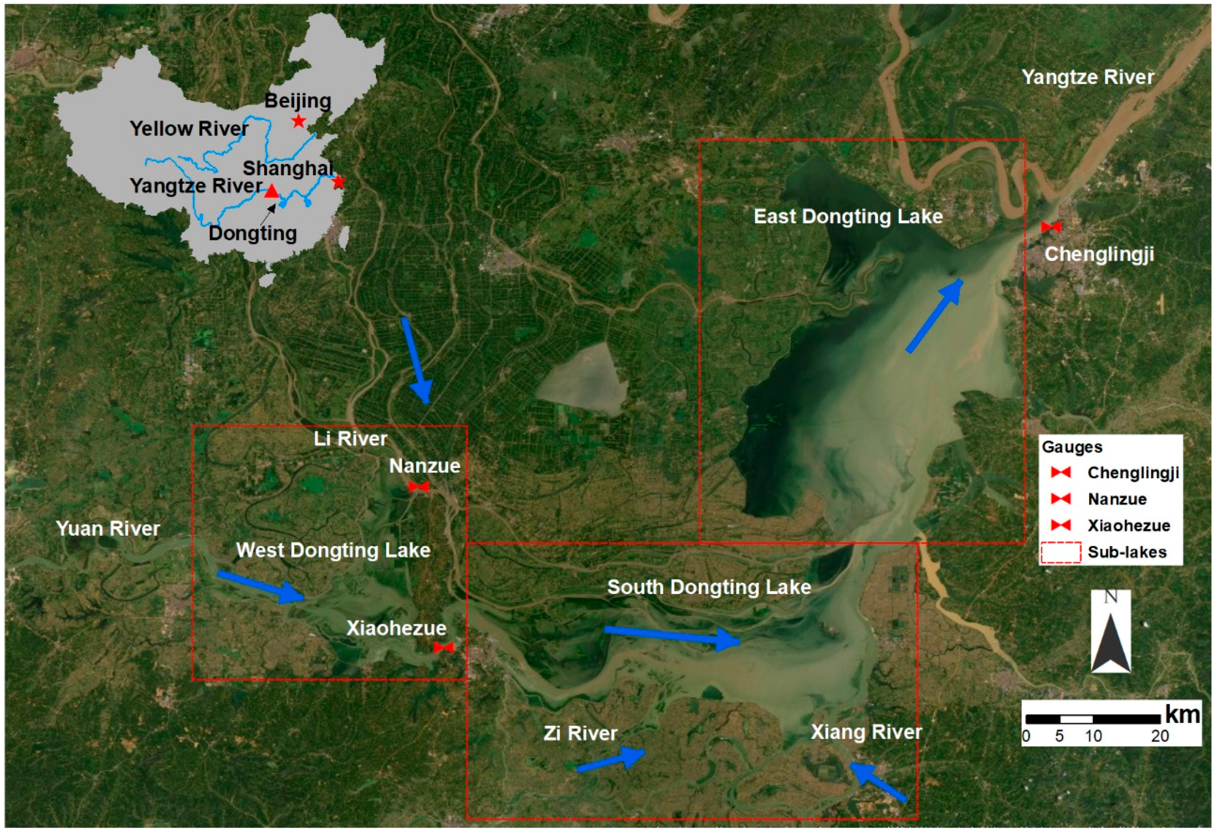
2.1. Study Site

The Dongting Lake (28°30′N–30°20′N, 111°40′E–113°10′E, hereafter referred as the Lake) is the second largest freshwater wetland complex in China, consisting a mosaic of permanent lakes and ephemeral swamps and floodplains that are interconnected through a network of channels and streams. It is located within the middle Yangtze River catchment of China (Figure 1) in a subtropical humid zone. Precipitation deceases from south to north with basin average annual total of 1400 mm. Temperature variation within the basin is relatively small and the mean summer and mean winter temperatures are 28.0 °C and 6.7 °C, respectively.

The Lake has three main water supply: escaping flows from the Yangtze through the “Three Outfalls”, inflows from four major tributaries (i.e., Li, Yuan, Zi, and Xiang), and local rainfall and runoff. The Lake discharges into the Yangtze through the only outlet channel located at northeast corner, and the flow was gauged at Chenglingji (Figure 1). The entire lake was divided into three sub-lakes, West Dongting Lake (WDTL), South Dongting Lake (SDTL), and East Dongting Lake (EDTL) (Figure 1), mainly due to the administrative boundary. The sub-lakes are connected through braided streams. In a typical year, lake water level starts to rise from early March and reaches peak at July, when most wetlands are inundated. When flood recedes in late September, vast mudflats and shallow lakes emerge, providing opportunity for plants to colonize and develop, which in turn provides foraging areas for wintering migratory birds, such as the greater white-fronted goose (Anser albifrons) and the tundra swan (Cygnus columbianus).

The water level in the Lake is characterized by large seasonal fluctuation: it can be up to 9.5 m at the inlet (Nanzue) and to 16.7 m at the outlet (Chenglingji) (Figure 1). The dramatic water level dynamics maintains a unique vegetation community zonation along the elevation gradient (

Table 1. Main wetland types in Dongting Lake.

Wetland Type	Key Species	Flood Requirement	Ecological Importance
Forested Wetlands	Populus nigra, Salix triandra	Tolerant short-term inundation	Non-native species for commercial planting
Reed marshes	Phragmites australis, Phalaris arundinacea, Miscanthus sacchariflorus	Can survival occasional, prolonged flooded	A typical wetland plant community, providing habitat for a range of wildlife, such as herons.
Wet meadows	Polygonum hydropiper Oenanthe javanica Carex brevicuspis	Shallow, periodic flooded	A typical wetland plant community, providing foraging habitat for migratory water birds (e.g., geese and cranes) and breeding structure for fish
Mudflat	-	Periodic flooded	Habitat for migratory water birds (e.g., geese and shorebirds)
Permanent water	Vallisneria natans Ceratophyllum demersum Hydrilla verticillata	-	Habitat for fish and migratory water birds (e.g., ducks and swan)

), ranging from permanent waters with submersed macrophytes to the forested wetlands with almond willow (Salix triandra) and forest plantation of black poplar (Populus nigra).

The Lake experienced a long history of land reclamation and the alternation of the natural flow regimes, especially after the Three Gorges Dam. These human disturbances have dramatically reduced the lake capacity [63] and changed the flow seasonality [62], resulting significant difference in wetland distribution [13] with potentially detrimental ecological consequences, such as losing wintering ground for migratory water birds [12] and reducing fish diversity [64]. Thus, wetland conservation is a major challenge to the ecological integrity of the Lake due to the increasing threats of water regime alternations [12,62].

With increasing acknowledgement of the importance of wetlands to sustaining the goods and services of the Lake, conservation actions, such as converting croplands to wetlands, breaching artificial levees, and removing poplar plantation, are practiced in the Dongting areas. In this study, we map the annual distribution of key wetland types in the Lake over a 20-year period (2000~2019) to explore the impacts of hydrological alternation and land-use change on wetland transition.

2.2. Data Source and Preparation

2.2.1. MODIS Enhanced Vegetation Index (EVI)

Enhanced vegetation Index (EVI) time series [65] from 2000 to 2019 downloaded from NASA EOSDIS LP DAAC (Earth Observing System Data and Information System, Land Processes Distributed Active Archive Center, https://earthdata.nasa.gov/eosdis/daacs/lpdaac). We used the “optimized” vegetation index EVI instead of NDVI (Normalized Difference Vegetation Index), as it enhances the vegetation signal with improved sensitivity in high biomass regions [66].

As some pixels have missing data due to cloud, we first applied a cubic smoothing spline [67] to all pixels with missing data to generate regular 16-day time series of EVI from 18 February 2000 to 24 May 2020. There are two phases of grassy vegetation development in a typical water year in the Lake driven by seasonal water level fluctuation and climate [68]. To fully account for the growth dynamics, we divided the yearly EVI time series into two: one for the water rise phase (i.e., December to May) and one for water recession phase (June to November). For each phase, we calculated a monotonic growth trend (Trend₁ and Trend₂) as Theil-Sen slope [69]. Based on the nonparametric Kendall tau statistic [70], the value of all grids with no significant trend (p > 0.05) was replaces with zero. In addition, we calculated four more annual summary metrics, the maximum, mean, minimum, and intra-annual standard deviation, making a total of six EVI-derived variables to capture the land-cover phenology of each grid. We used package spatialEco [71] and Raster package [72] within R version 3.6.1 [73] for all raster manipulations and calculations.

2.2.2. Geomorphological Variables

Inclusion of topographic metrics can improve the accuracy of wetland mapping [74]. We computed a range of geomorphological variables from DEM (digital elevation model). The DEM with 1:10,000 spatial scale was provided by the Changjiang Water Resource Commission.

• One and two degree detrended DEM (Figure 2): the residuals of the linear regression of poly (x, y) with degree of 1 and 2,

  $$DE{M}_{detrend1}=DE{M}_{mean}+X+Y+\epsilon$$

  (1)

  $$DE{M}_{detrend2}=DE{M}_{mean}+a_1{X}^2+a_{2}XY+a_3{Y}^2+a_{4}X+a_{5}Y+Ɛ$$

  (2)

  where Equation (1) for first order detrended elevation and Equation (2) for second order detrended DEM, and where x and y are the longitude and latitude of central of a grid and $DE{M}_{mean}$ is the global mean DEM.
• CTI (Compound Topographic Index) [75]—a steady state wetness index calculated using

  $$cti=\ln \left[\frac{\alpha }{\tan \theta }\right]$$

  (3)

  where α = catchment area [(flow accumulation + 1) × (pixel area in m²)], and θ is the slope angle in radians.
• Local deviation from global (LDFG) [76]:

  $$LDFG=\overline{y}-y_i$$

  (4)

  where $\overline{y}$ is global mean elevation of a 3 × 3 window, and $y_i$ is the elevation of grid i.
• TPI (Topographic Position Index) [77]: the difference between the value of a cell and the mean value of its 8 surrounding cells

  $$TPI=h-h_{mean}$$

  (5)

These variables are computed using the ‘spatialEco’ package by Evans and Ram [71] and package ‘Spatstat’ by Baddeley [78]. All these topographic variables were resampled to 250 m.

To limit the effect of collinearity on clustering, we excluded the highly correlated variables. We randomly selected 20,000 points (with the constraint of 250 m apart) within the study area (about 25% of the total grids) and extracted all EVI and geomorphological variables using these random points. We calculated the Pearson correlation coefficients r between every pair of the variables. For the pair with absolute r greater than 0.75, we kept only one variable for further analysis. This procedure resulted in a set of eight variables, namely Detrend.1, CTI, TPI, Trend₁, Trend₂, EVI_mean, EVI_min, and EVI_sd. We built a raster brick with these eight layers (each layer is a raster for a variable). The raster brick was then normalized for further k-means clustering.

2.3. Wetland Clustering

2.3.1. Assessing Clustering Tendency

Before clustering, we assessed the clustering tendency of the dataset using the Hopkins statistic [79]. The Hopkins statistic tests the spatial randomness of the data, ranging from 0 (uniformly distributed) to 1 (highly clustered), and a spatially random data tend to have a value of 0.5. The Hopkins statistics for our dataset ranged from 0.88 to 0.95, and the Hopkins statistic for majority of years is over 0.90 (

Table 2. Cluster tendency and silhouette width for the optimal number of clusters for each year based on 5000 random samples.

Year	Tendency	Average Width	No. of Clusters (Elbow)	No. of Clusters (Silhouette)	No. of Clusters (Gap Statistics)
2000	0.90	0.39	3	4	5
2001	0.90	0.42	3	3	7
2002	0.93	0.48	3	3	3
2003	0.94	0.43	3	3	3
2004	0.90	0.45	3	3	10
2005	0.93	0.44	3	3	4
2006	0.90	0.45	4	3	4
2007	0.91	0.47	3	3	3
2008	0.92	0.49	3	2	7
2009	0.95	0.44	3	2	5
2010	0.94	0.39	3	3	3
2011	0.90	0.44	3	3	6
2012	0.96	0.43	3	3	1
2013	0.94	0.47	3	3	3
2014	0.88	0.43	3	3	3
2015	0.94	0.45	3	3	4
2016	0.94	0.42	3	3	7
2017	0.91	0.38	4	3	6
2018	0.92	0.51	3	3	5
2019	0.93	0.46	3	3	3

), far above the threshold of 0.5, indicating that the land grids are well clustered and highly separable.

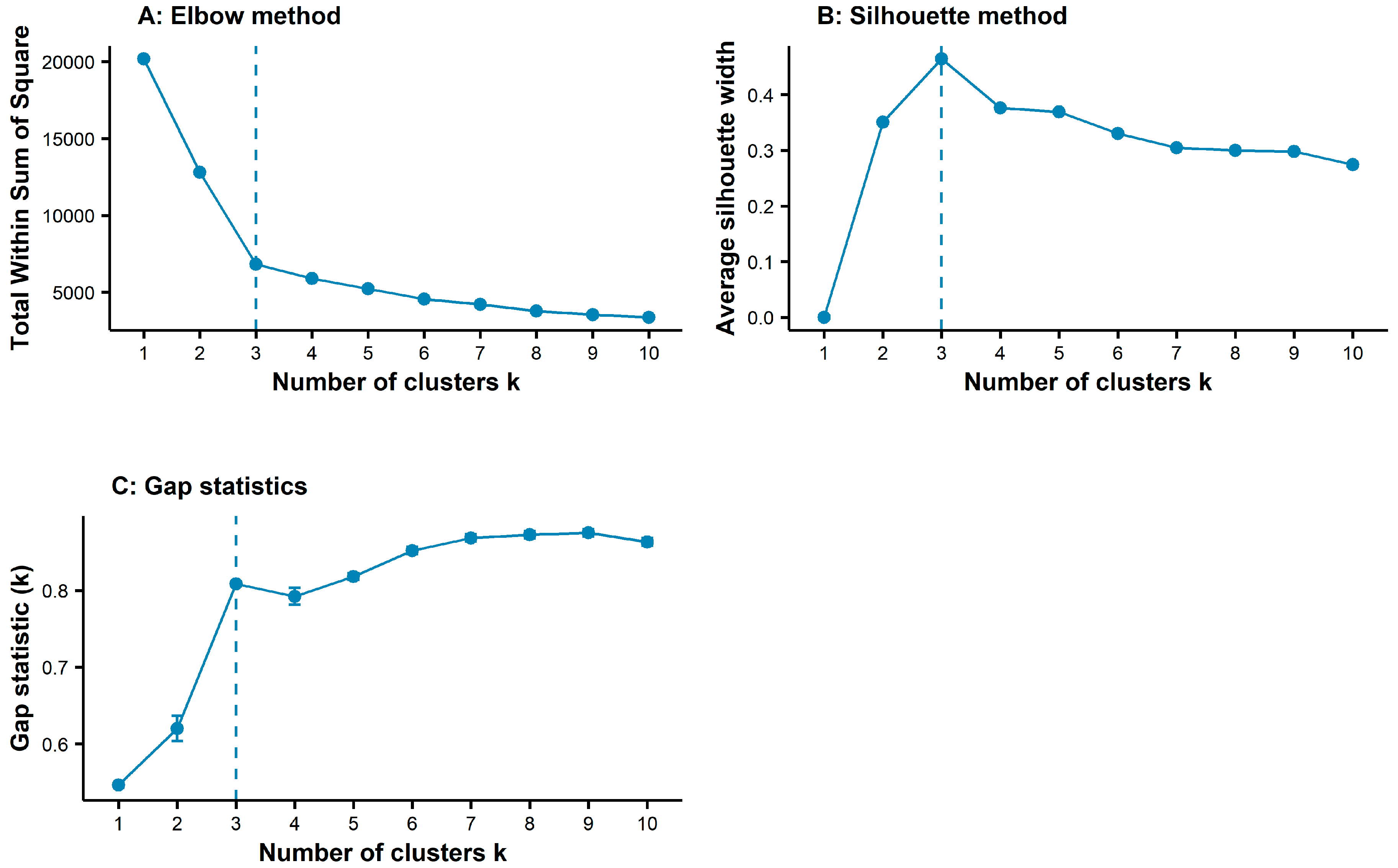
2.3.2. Estimating the Optimal Number of Clusters

The k-medoids clustering requires a prior specification of the number of clusters to be generated. There are many indices developed to determine the optimal number of clusters [80]. However, the optimal number of clusters is somehow subjective and depends on the method used for measuring similarities and the indices used for partitioning.

In this study, we use three methods to estimate the optimal number of clusters: elbow, gap statistic [81], and average silhouette method. The elbow method minimizes the total within-cluster sum of square (WSS), which measures the compactness of the clustering. The elbow method looks at the total WSS as a function of the number of clusters: the number of clusters is selected in such a way so that adding another cluster does not improve much better the total WSS (the elbow point). The gap statistic method compares the change in with-cluster dispersion with the expected dispersion, which is defined through bootstrapping simulation (n = 500 in this study) from a reference distribution. The average silhouette method computes the average silhouette of observations for different values of k. The optimal number of clusters k is the one that maximize the average silhouette width (see below) over a range of possible values for k [82]. The three methods were applied to a subset of 5000 randomly selected observations.

2.3.3. CLARA an Extension of k-Medoids Algorithm (PAM)

We used k-medoids or Partitioning Around Medoids (PAM), one of the most popular unsupervised learning algorithms in data mining [83,84], to delineate vegetation condition class in the Lake. PAM is a robust alternative to k-means for partitioning a dataset into clusters of observation, as it is less sensitive to noise and outliers [82], which are the features of our predictor variables. The goal of the PAM algorithm is to find a sequence of objects (medoids) that are centrally located in clusters by minimizing the average dissimilarity of objects to their closest selected object [82].

The dataset is very large (i.e., 52,498 × 8), preventing the direct application of PAM to the entire dataset due to RAM storage and computing time problems. Therefore, we use CLARA (i.e., Clustering Large Applications) [85,86], which is an extension to PAM designed to deal with data containing a large number of observations. Instead of finding medoids for the entire dataset, CLARA considers a subset of random samples from the original data with a fixed size (5100, about 10% of the original dataset in our study) and applies the PAM algorithm to generate an optimal set of medoids. The procedure of sampling and clustering is repeated for a pre-specified number of times (1000 in this study) in order to minimize the sampling bias. The final clustering results correspond to the set of medoids with the minimal cost, defined as

$$Cost\left(M,D\right)=\frac{{\sum }_{i=1}^{n}dissimilarity(O_i, rep(M,O_i))}{n}$$

(6)

where M is a set of selected clusters, dissimilarity (O_i, O_j) is the dissimilarity of objects O_i and O_j, and rep (M, O_i) is a medoid in M that is closest to O_i.

CLARA is conducted with the “clara” function from the cluster package [87].

2.4. Clustering Validation

We first assess the clustering by visually inspecting the partitioning result using the function fviz_cluster in factoextra package [88], which produces a scatter plot of datapoints colored by cluster numbers. We then employed both internal and external cluster validation measurements to quantify the cluster results.

2.4.1. Internal Validation

We calculated two indicators of each cluster map, i.e., silhouette width and isolation, to assess the quality of clustering.

The silhouette analysis measures how well an observation is clustered, and it estimates the average distance between clusters as

$$S_i=\frac{b_i-a_i}{\max \left(b_i,a_i\right)}$$

(7)

where a_i is the average dissimilarity between observation i and all other points of the cluster to which i belongs. For all other clusters C, d(i,C) is average dissimilarity of i to all observations of C, and b_i is the smallest of these d(i,C). b_i can be interpreted as the dissimilarity between i and its “neighbor” cluster, i.e., the nearest one to which it does not belong.

A large S_i (approaching 1) are very well clustered. A small S_i (around 0) means that the observation lies between two clusters. Observations with a negative S_i are probably placed in the wrong cluster. Isolation is computed as the ratio of the maximal dissimilarity between the observations in the cluster and the cluster’s medoid and the minimal dissimilarity between the cluster’s medoid and the medoid of any other cluster. If this ratio is small, the cluster is well-separated from the other clusters.

2.4.2. Map Validation

We compared the clustering maps with two existing vegetation maps for the Dongting area (2009 and 2013), which were based on Landsat image segmentation and validated by ground-truthing. The vegetation maps have 7 classes, i.e., water, mudflat, grassland, reed, poplar tree, other trees, and others (including roads, human settlement, and croplands). We combined these classes to the three clusters in our wetland type maps, namely shallow waters (include waters and mudflats), wet meadow, and rushes (combination of reed marshes and forests). As reed and forest are both subject to harvesting in winter and regeneration (reed) and replantation (poplar tree) in spring, it is difficult to distinguish without extensive field survey. Moreover, more and more poplar plantations are abandoned due to the ongoing “returning cropland to wetland” policy and are gradually colonized by reed, we grouped reed and forest together as one class. The combined 30 m vegetation maps were then aggregated to 250 m. We conducted a cell to cell comparison and computed the Cohen’s Kappa index [89] as a measurement of the degree of agreement for both years.

3. Results

3.1. Optimal Number of Clusters

For most of the years, both elbow and average silhouette methods are consistent, indicating that the optimal number of clusters was three (Table 2, Figure 3). However, the gap statistics often provided different answers. For example, the optimal k for 2004 was 10 according to gap statistics, while both elbow and silhouette methods suggested k = 3 (Table 2). To be consistent, we selected three as the optimal number of clusters for all years.

3.2. Accuracy of the Classification

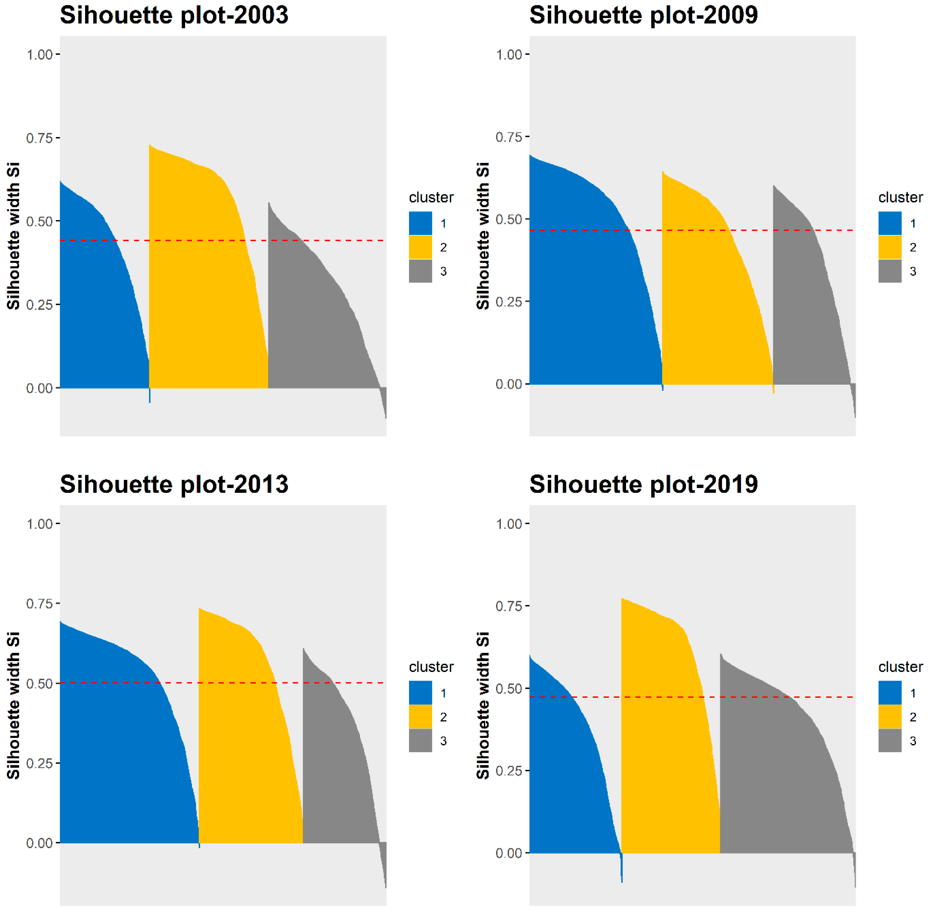
3.2.1. Internal Clustering Validation

The average silhouette width ranged from 0.39 in 2017 to 0.52 in 2018, and the isolation index was small as well (ranged from 0.98 in 2002 to 2.90 in 2012 (

Table 3. Silhouette width (si) and isolation index for the CLARA (Clustering Large Applications) clustering.

Year	Average		Shallow Waters		Wet Meadows		Rushes
	Si	Isolation	Si	Isolation	Si	Isolation	Si	Isolation
2000	0.42	1.66	0.55	1.12	0.37	1.97	0.32	1.90
2001	0.44	1.48	0.59	1.15	0.32	1.29	0.43	1.99
2002	0.50	0.98	0.65	0.80	0.39	1.05	0.42	1.08
2003	0.44	2.21	0.57	1.40	0.31	3.67	0.44	1.57
2004	0.46	1.22	0.61	0.95	0.31	1.41	0.47	1.29
2005	0.43	1.84	0.59	1.37	0.23	2.41	0.51	1.74
2006	0.43	1.03	0.60	0.86	0.23	1.17	0.52	1.06
2007	0.46	1.13	0.59	0.86	0.34	1.41	0.48	1.11
2008	0.43	1.41	0.61	1.48	0.18	1.83	0.55	0.94
2009	0.47	1.58	0.45	1.06	0.38	2.45	0.53	1.23
2010	0.41	2.47	0.52	1.88	0.34	2.52	0.38	3.00
2011	0.47	1.28	0.57	0.86	0.40	1.25	0.44	1.75
2012	0.44	2.90	0.60	0.91	0.25	4.75	0.47	3.05
2013	0.50	1.80	0.56	1.03	0.37	2.04	0.53	2.32
2014	0.44	1.39	0.58	1.09	0.30	1.40	0.44	1.69
2015	0.49	1.67	0.60	1.24	0.33	1.72	0.49	2.04
2016	0.42	1.97	0.62	1.18	0.19	3.01	0.44	1.73
2017	0.39	2.41	0.60	2.08	0.18	2.59	0.40	2.56
2018	0.52	1.00	0.63	0.84	0.43	1.01	0.48	1.15
2019	0.47	1.45	0.62	1.02	0.39	1.89	0.42	1.44

)), suggesting the clustering algorithm separated the grids well. For individual classes, water areas were generally better distinguished than grasslands and territorialized areas, as the silhouette width was comparably larger and the isolation index was smaller for water than for the others (Table 3).

The visual inspection of the clustering showed that the separation of clusters was well performed (Figure 4 and Figure 5). The first two PCA (principal component analysis) axes explained more than 85% of the difference in the EVI metrics of the grids (Figure 4). Most critically, there are very few overlaps of the convex hull of the clusters. The silhouette plots also showed that very few grids were wrongly placed (i.e., negative si value, Figure 5).

3.2.2. Validation of Clustering with Vegetation Maps

The comparisons with vegetation maps showed that the unsupervised machine-learning technique achieved satisfactory results for both 2009 and 2013 (

Table 4. Summary of clustering accuracy in comparison with vegetation maps.

Year	Overall Accuracy	Kappa	Shallow Waters		Wet Meadows		Rushes
			UA	PA	UA	PA	UA	PA
2009	0.8519 (0.8483, 0.8554)	0.7731	0.9356	0.8438	0.9287	0.858	0.9108	0.8544
2013	0.8768 (0.8753, 0.8818)	0.8116	0.9473	0.8761	0.9316	0.8787	0.9413	0.8806

UA = user’s accuracy; PA = producer’s accuracy.

). Although the performance is slightly better for 2013 (Table 4), the Kappa coefficient was over 0.75 for both years, indicating substantial performance, according to Landis and Koch [90]. The overall accuracy, which defines the percentage of correctly classified instances, was also high (greater than 85%, Table 4) for both years.

For individual class, there was no systematic misclassification as the balanced accuracy for each class was comparable, which was confirmed by visually comparing the maps. The small patches of wet meadows within large area of rushes distinguished by the wetland distribution maps based on Landsat image were generally absent from the map produced using MODIS data, presenting the majority of mismatches. In addition, both the producer’s and user’s accuracy were high and comparable (Table 4).

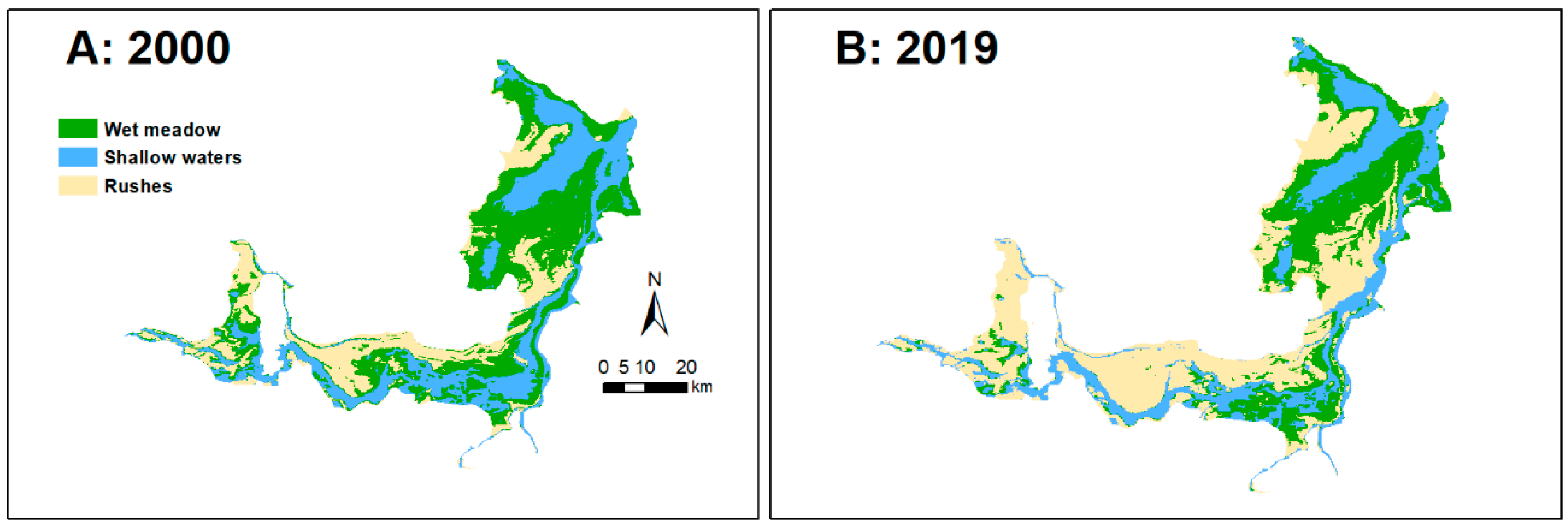
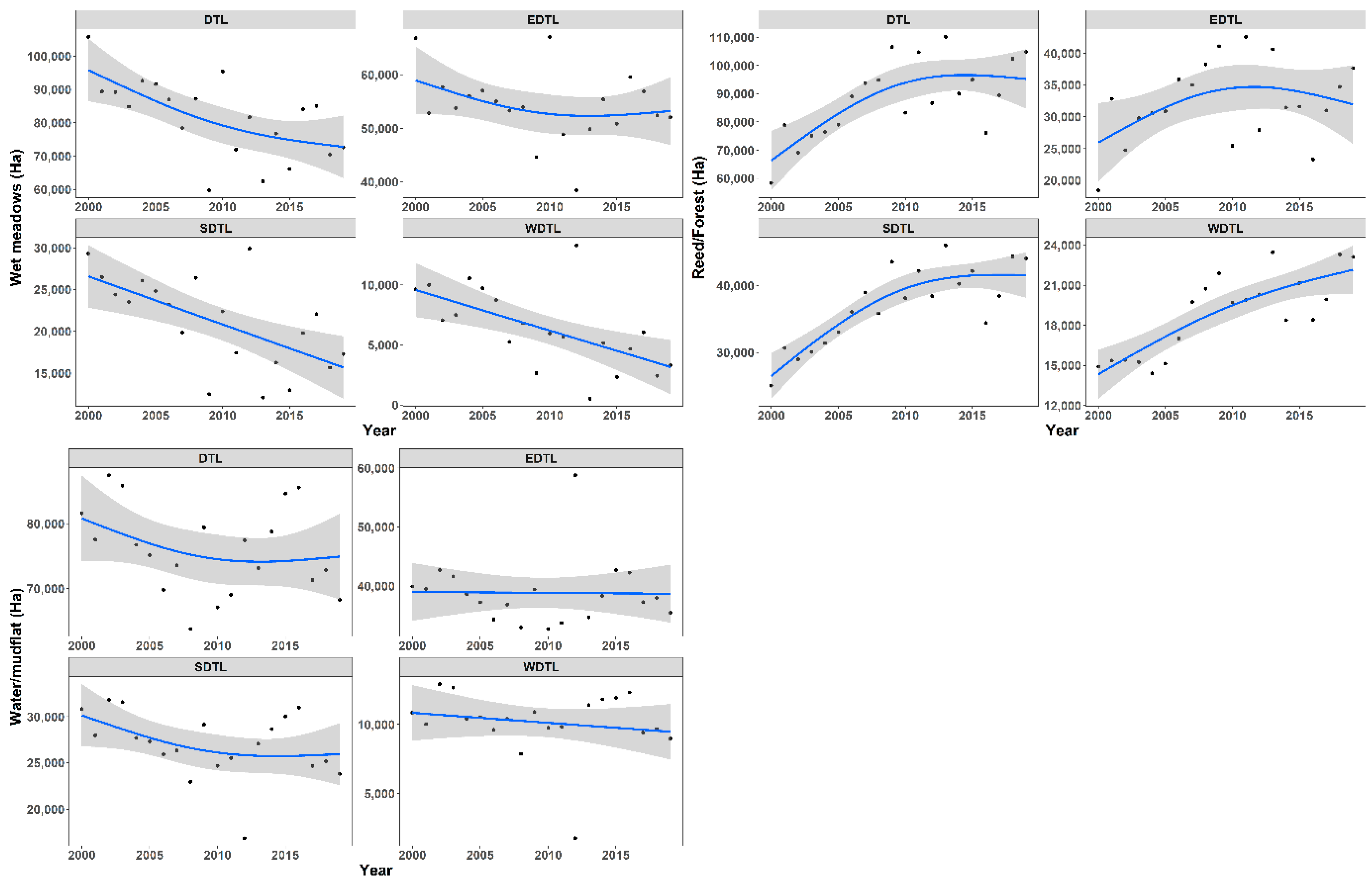
3.3. Changes of Wetland Extent

The overall dynamics of wetland transition during 2000 to 2019 in Dongting Lake was the encroachment of reeds and forests into wet meadows, and to less extent, the colonization of wet meadows in mudflats and waters (Figure 6). While the encroachment of reeds (forests) was widespread across the Lake, the wet meadow colonization mainly occurred in EDTL, probably because of the limited availability of shallow waters and mudflats in WDTL and SDTL.

The overall change of wetland extent and distribution for the 20-year study period in Dongting Lake is presented in Figure 6. During the 20-year period, rushes increased substantially in the expense of wet meadows and shallow water/mudflat (

Table 5. Gain and loss of wetlands in Dongting Lake and its sub-lakes during 2000–2019.

	Wetland Type	Change Rate (ha/yr)	Change (%)
Lake	Water/mudflat	−666.60	−16.34
	Wet meadows	−1657.95	−31.35
	Rushes	2322.85	79.53
East Dongting Lake	Water/mudflat	−222.95	−11.17
	Wet meadows	−739.45	−22.13
	Rushes	961.75	104.32
South Dongting Lake	Water/mudflat	−350.45	−22.74
	Wet meadows	−601.40	−41.03
	Rushes	950.20	75.81
West Dongting Lake	Water/mudflat	−93.15	−17.18
	Wet meadows	−317.05	−65.78
	Rushes	410.90	55.13

). For the entire system, 31.35% of wet meadows was lost at a rate of 1675.95 ha year⁻¹, while rushes increased nearly 80% at an annual rate of 2322.85 ha. A comparison of wetland distribution maps in 2000 and 2019 found that growth (i.e., expansion of existing patches) and colonization (i.e., establishing new colonies) of phragmite were both responsible for the rapid gain of rush land. Compared with wet meadows, the loss of water/mudflat was less striking (16.34% loss at 666.60 ha year⁻¹). For individual sub-lakes, the trends of loss and gain were similar although varied in change rates. The loss of wet meadows was most severe in WDTL at the upstream, where up to 65.78% was replaced with rushes (Table 5). The fastest gain of rushes occurred in EDTL, where area of rushes increased 104.32% (an increasing rate of 961.75 ha year⁻¹) during the 20-year period. Until 2019, although there was still large area of shallow waters/mudflats in WDTL, there was no area of wet meadows large enough to support viable population of watering geese in WDTL (Figure 6). This is also true for SDTL, where large patches of wet meadow were pushed to the downstream deltas, where Zi River and Xiang River enter the Lake (Figure 6).

For the entire lake, the overall increasing trend of rushes and decreasing trend of wet meadow were clear, whereas there was no clear trend for water/mudflat (Figure 7). However, the change rates were not spatially consistent. Moreover, the dynamics for wetland types also varied. The overall pattern of wet meadow dynamics was decreasing and was mainly driven by the changes in WDTL and SDTL (Figure 7). The decreases in the extent of wet meadows were almost linear in WDTL and SDTL, and the rate of changes were comparable indicated by the smooth lines. However, in EDTL, the fitted smooth line indicated the decrease was sharper before 2009 (although at a much slower rate that in WDTL and SDTL) but flatted till the end of study period. In contrast, the general dynamics of rushes was increasing although the trend was not linear. In SDTL (and the whole lake), the colonization of reed and forest began to slow down after 2009, whereas the increasing rate remained high until the end of the study period in WDTL. However, in EDTL, the fitted smooth line suggested that the increasing trend of rushes was reversed after 2009 (Figure 7).

4. Discussion

For effective wetland restoration and management, it is essential to consider them as a dynamic landscape unit rather than a static land-cover type [11], which requires periodic mapping to monitor their spatiotemporal dynamics [44]. In this study, we developed and tested a framework that uses topographic variables derived from DEM and land-surface phenological metrics based on a MODIS EVI time series to generate annual wetland maps for a large subtropical monsoon wetland complex. The validation results showed that the accuracy of our approach was consistent and comparable to that of the time-consuming manual Landsat image segmentation with high Kappa coefficient of agreement and accuracy for both overall and individual classes (Table 4). Our framework provides a fast and cost-efficient alternative to monitor ecological responses in a rapidly changing environment, which is key to making effective conservation decisions [91].

MODIS data in 250 m resolution have been widely used in large-scale land-cover mapping [29,92,93]. The trade-off in spatial and temporal resolution of MODIS data provides a unique capability to distinguish annually recurring temporal patterns and to map land-cover types without the need for expensive ground data [93]. The regularity of the 16-day MODIS products provides a major advantage for capturing the land-surface phenology [50]. This is particular useful to study dynamic landscapes that have distinct seasonal patterns including croplands [92,93] and floodplains [44,94,95]. The Hopkins statistic [79] indicated that pixels with annual metrics of land-surface phenology and topographic features have very high cluster tendency (>0.9, Table 2), providing a solid basis for using unsupervised clustering. However, the results of all three employed methods (i.e., elbow, gap statistic, and average silhouette) suggested that our approach might not be consistent for finer (i.e., above three classes) clustering. Powell et al. [42] suggested that discrimination limit for semi-arid floodplain using Landsat based NDVI metrics was four classes, beyond which the performance was significantly deteriorated.

The widespread and rapid loss of wet meadows to rushes in the Lake, particularly within the upstream section (i.e., WDTL and SDTL) reflects the global trend of encroachment of Common Reed (Phragmites australis), a semi-aquatic species, into freshwater and blackish wetlands in subtropical and temperate climates [96,97]. The encroachment of phragmites is associated with increasing nutrient level, altered water regimes, and human disturbances [98,99]. During 2003–2009, the rate of rush expansion was very high (Figure 7), coincident to the period of TGD impounding. This finding suggests that the TGD accelerated the xerophilization trend in the Lake. Large patches of wet meadows (often in hundreds to thousands ha) in the Lake provide irreplaceable winter foraging habitats for hundreds and thousands of migratory water birds, especially ducks and geese [12], representing the most significant ecological asset in the region. In contrast, water birds avoid tall and dense phragmites marshes [100]. Moreover, the rushes offer poor-quality habits for larval and juvenile fish [101]. Thus, the encroachment of rushes into wet meadows presents a real ecological threat to local and regional biodiversity, which requires urgent remediation management actions. This urgency is even more pressing for WDTL and upstream of SDTL, where rush expansion was almost linear from 2000 to 2019, and there is no sign of slowing down.

5. Conclusions and Management Implications

Periodically mapping of the distribution and extent of wetlands subjected to natural and/or anthropogenic disturbances is a vital task to identify long-term trends and short-term variations for sustainable natural resource management. In this study, we applied an unsupervised machine-learning algorithm—the k-medoids algorithm—to re-construct the long-term floodplain wetland dynamics using land phenology metrics derived from the 16-day composite MODIS EVI time series. Despite the relatively coarse spatial resolution of MODIS data, our approach achieved comparable performance to the time-consuming satellite image segmentation method with a Kappa coefficient of agreement greater than 0.75 and an overall accuracy over 85%. The framework offers a fast and cost-effective alternative to monitor spatial distribution dynamics of wetland in the Dongting Lake and may be applicable to other large river floodplain systems across the world. With the re-constructed annual wetland distribution maps, we found widespread and continuous encroachment of rushes into wet meadows, the most significant ecological asset in the region. In addition, to a much lesser extent, wet meadows have expanded into shallow waters. During the past two decades, 31.35% of wet meadows in Dongting Lake were lost at a rate of 1675.95 ha year⁻¹, while the area of rushes increased by 79.53% of rushes at an annual rate of 2322.85 ha. Moreover, we identified a period of accelerated rush encroachment (i.e., 2003–2009), which was coincident to the TGD impounding. These findings highlight the rapid disappearing of the highly valuable wetlands caused by river regulations, representing a pressing ecological threat to local and regional biodiversity.

References

1. Davidson, N.C.; Finlayson, C.M. Extent, regional distribution and changes in area of different classes of wetland. Mar. Freshw. Res. 2018, 69, 1525–1533. [Google Scholar] [CrossRef] [Green Version]
2. Lehner, B.; Döll, P. Development and validation of a global database of lakes, reservoirs and wetlands. J. Hydrol. 2004, 296, 1–22. [Google Scholar] [CrossRef]
3. Silva, T.S.F.; Costa, M.P.F.; Melack, J.M. Spatial and temporal variability of macrophyte cover and productivity in the eastern Amazon floodplain: A remote sensing approach. Remote Sens. Environ. 2010, 114, 1998–2010. [Google Scholar] [CrossRef]
4. Han, X.; Chen, X.; Feng, L. Four decades of winter wetland changes in Poyang Lake based on Landsat observations between 1973 and 2013. Remote Sens. Environ. 2015, 156, 426–437. [Google Scholar] [CrossRef]
5. Wang, H.Z.; Liu, X.Q.; Wang, H.J. The Yangtze River-Floodplain: Threats and rehabilitation. In American Fisheries Society Symposium; Chen, Y., Duane, C., Jackson, J.R., Chen, D., Li, Z., Kilgore, K.J., Phelps, Q., Eggleton, M.A., Eds.; American Fisheries Society: Bethesda, MD, USA, 2016; pp. 263–291. [Google Scholar]
6. McCarthy, J.M.; Gumbricht, T.; McCarthy, T.; Frost, P.; Wessels, K.; Seidel, F. Flooding patterns of the Okavango Wetland in Botswana between 1972 and 2000. Ambio 2003, 32, 453–457. [Google Scholar] [CrossRef]
7. Cai, Y.; Li, X.; Zhang, M.; Lin, H. Mapping wetland using the object-based stacked generalization method based on multi-temporal optical and SAR data. IJAEO 2020, 92, 102164. [Google Scholar]
8. Parrens, M.; Bitar, A.A.; Frappart, F.; Paiva, R.; Wongchuig, S.; Papa, F.; Yamasaki, D.; Kerr, Y. High resolution mapping of inundation area in the Amazon basin from a combination of L-band passive microwave, optical and radar datasets. IJAEO 2019, 81, 58–71. [Google Scholar] [CrossRef]
9. Silio-Calzada, A.; Barquin, J.; Huszar, V.L.M.; Mazzeo, N.; Mendez, F.; Alvarez-Martinez, J.M. Long-term dynamics of a floodplain shallow lake in the Pantanal wetland: Is it all about climate? Sci. Total Environ. 2017, 605–606, 527–540. [Google Scholar] [CrossRef]
10. Yang, L.; Wang, L.; Yu, D.; Yao, R.; Li, C.a.; He, Q.; Wang, S.; Wang, L. Four decades of wetland changes in Dongting Lake using Landsat observations during 1978–2018. J. Hydrol. 2020, 587. [Google Scholar] [CrossRef]
11. Taddeo, S.; Dronova, I. Indicators of vegetation development in restored wetlands. Ecol. Indic. 2018, 94, 454–467. [Google Scholar] [CrossRef]
12. Guan, L.; Lei, J.; Zuo, A.; Zhang, H.; Lei, G.; Wen, L. Optimizing the timing of water level recession for conservation of wintering geese in Dongting Lake, China. Ecol. Eng. 2016, 88, 90–98. [Google Scholar] [CrossRef]
13. Jing, L.; Lu, C.; Xia, Y.; Shi, L.; Zuo, A.; Lei, J.; Zhang, H.; Lei, G.; Wen, L. Effects of hydrological regime on development of Carex wet meadows in East Dongting Lake, a Ramsar Wetland for wintering waterbirds. Sci. Rep. 2017, 7, 41761. [Google Scholar] [CrossRef] [PubMed] [Green Version]
14. Nilsson, C.; Reidy, C.A.; Dynesius, M.; Revenga, C. Fragmentation and flow regulation of the world’s large river systems. Science 2005, 308, 405–408. [Google Scholar] [CrossRef] [Green Version]
15. Pekel, J.F.; Cottam, A.; Gorelick, N.; Belward, A.S. High-resolution mapping of global surface water and its long-term changes. Nature 2016, 540, 418–422. [Google Scholar] [CrossRef] [PubMed]
16. Reid, A.J.; Carlson, A.K.; Creed, I.F.; Eliason, E.J.; Gell, P.A.; Johnson, P.T.J.; Kidd, K.A.; MacCormack, T.J.; Olden, J.D.; Ormerod, S.J.; et al. Emerging threats and persistent conservation challenges for freshwater biodiversity. Biol. Rev. Camb. Philos. Soc. 2019, 94, 849–873. [Google Scholar] [CrossRef] [Green Version]
17. Tockner, K.; Pusch, M.; Borchardt, D.; Lorang, M.S. Multiple stressors in coupled river-floodplain ecosystems. Freshwat. Biol. 2010, 55, 135–151. [Google Scholar] [CrossRef]
18. Feyisa, G.L.; Meilby, H.; Fensholt, R.; Proud, S.R. Automated Water Extraction Index: A new technique for surface water mapping using Landsat imagery. Remote Sens. Environ. 2014, 140, 23–35. [Google Scholar] [CrossRef]
19. United Nations. New UN Decade on Ecosystem Restoration Offers Unparalleled Opportunity for Job Creation, Food Security and Addressing Climate Change. 2019. Available online: https://www.unenvironment.org/news-and-stories/press-release/new-undecade-ecosystem-restoration-offers-unparalleledopportunity (accessed on 21 May 2010).
20. Latrubesse, E.M.; Arima, E.Y.; Dunne, T.; Park, E.; Baker, V.R.; d’Horta, F.M.; Wight, C.; Wittmann, F.; Zuanon, J.; Baker, P.A.; et al. Damming the rivers of the Amazon basin. Nature 2017, 546, 363–369. [Google Scholar] [CrossRef]
21. Arthington, Á.H.; Naiman, R.J.; Mcclain, M.E.; Nilsson, C. Preserving the biodiversity and ecological services of rivers: New challenges and research opportunities. Freshwat. Biol. 2010, 55, 1–16. [Google Scholar] [CrossRef] [Green Version]
22. Jungwirth, M.; Muhar, S.; Schmutz, S. Re-establishing and assessing ecological integrity in riverine landscapes. Freshwat. Biol. 2002, 47, 867–887. [Google Scholar] [CrossRef]
23. Qureshi, M.E.; Schwabe, K.; Connor, J.; Kirby, M. Environmental water incentive policy and return flows. WRR 2010, 46, 4. [Google Scholar] [CrossRef] [Green Version]
24. Guida, R.J.; Remo, J.W.F.; Secchi, S. Tradeoffs of strategically reconnecting rivers to their floodplains: The case of the Lower Illinois River (USA). Sci. Total Environ. 2016, 572, 43–55. [Google Scholar] [CrossRef]
25. Fang, Y.; Du, S.; Scussolini, P.; Wen, J.; He, C.; Huang, Q.; Gao, J. Rapid Population Growth in Chinese Floodplains from 1990 to 2015. Int. J. Environ. Res. Public Health 2018, 15, 1602. [Google Scholar] [CrossRef] [Green Version]
26. Hein, T.; Schwarz, U.; Habersack, H.; Nichersu, I.; Preiner, S.; Willby, N.; Weigelhofer, G. Current status and restoration options for floodplains along the Danube River. Sci Total Environ. 2016, 543, 778–790. [Google Scholar] [CrossRef]
27. Tockner, K.; Schiemer, F. Ecological aspects of the restoration strategy for a river-floodplain system on the Danube River in Austria. Glob. Ecol. Biogeogr. Lett. 1997, 6, 321–329. [Google Scholar] [CrossRef]
28. Alsdorf, D.; Han, S.-C.; Bates, P.; Melack, J. Seasonal water storage on the Amazon floodplain measured from satellites. Remote Sens. Environ. 2010, 114, 2448–2456. [Google Scholar] [CrossRef]
29. Chen, Y.; Huang, C.; Ticehurst, C.; Merrin, L.; Thew, P. An evaluation of MODIS daily and 8-day composite products for floodplain and wetland inundation mapping. Wetlands 2013, 33, 823–835. [Google Scholar] [CrossRef]
30. Palmer, M.A.; Bernhardt, E.S.; Allan, J.D.; Lake, P.S.; Alexander, G.; Brooks, S.; Carr, J.; Clayton, S.; Dahm, C.N.; Follstad Shah, J.; et al. Standards for ecologically successful river restoration. J. Appl. Ecol. 2005, 42, 208–217. [Google Scholar] [CrossRef]
31. Rodriguez-Gonzalez, P.M.; Albuquerque, A.; Martinez-Almarza, M.; Diaz-Delgado, R. Long-term monitoring for conservation management: Lessons from a case study integrating remote sensing and field approaches in floodplain forests. J. Environ. Manag. 2017, 202, 392–402. [Google Scholar] [CrossRef]
32. Christopher, L.; Lunetta, S. Wetland detection methods. In Wetland and Environmental Applications in GIS; Lyon, J.G., McCarthy, J., Eds.; Lewis: Boca Raton, FL, USA, 1996; pp. 249–284. [Google Scholar]
33. Pelletier, C.; Valero, S.; Inglada, J.; Champion, N.; Dedieu, G. Assessing the robustness of Random Forests to map land cover with high resolution satellite image time series over large areas. Remote Sens. Environ. 2016, 187, 156–168. [Google Scholar] [CrossRef]
34. Ullerud, H.A.; Bryn, A.; Halvorsen, R.; Hemsing, L.Ø. Consistency in land-cover mapping: Influence of field workers, spatial scale and classification system. Appl. Veg. Sci. 2018, 21, 278–288. [Google Scholar] [CrossRef] [Green Version]
35. Herold, M.; Mayaux, P.; Woodcock, C.E.; Baccini, A.; Schmullius, C. Some challenges in global land cover mapping: An assessment of agreement and accuracy in existing 1 km datasets. Remote Sens. Environ. 2008, 112, 2538–2556. [Google Scholar] [CrossRef]
36. Friedl, M.A.; McIver, D.K.; Hodges, J.C.F.; Zhang, X.Y.; Muchoney, D.; Strahler, A.H.; Woodcock, C.E.; Gopal, S.; Schneider, A.; Cooper, A.; et al. Global land cover mapping from MODIS: Algorithms and early results. Remote Sens. Environ. 2002, 83, 287–302. [Google Scholar] [CrossRef]
37. Cihlar, J. Land cover mapping of large areas from satellites: Status and research priorities. IJRS 2000, 21, 1093–1114. [Google Scholar]
38. Congalton, R.G.; Gu, J.; Yadav, K.; Thenkabail, P.; Ozdogan, M. Global land cover mapping: A review and uncertainty analysis. Remote Sens. 2014, 6, 12070–12093. [Google Scholar] [CrossRef] [Green Version]
39. Curtis, P.G.; Slay, C.M.; Harris, N.L.; Tyukavina, A.; Hansen, M.C. Classifying drivers of global forest loss. Science 2018, 361, 1108–1111. [Google Scholar] [CrossRef]
40. Teferi, E.; Bewket, W.; Uhlenbrook, S.; Wenninger, J. Understanding recent land use and land cover dynamics in the source region of the Upper Blue Nile, Ethiopia: Spatially explicit statistical modeling of systematic transitions. Agric. Ecosyst. Environ. 2013, 165, 98–117. [Google Scholar] [CrossRef]
41. Palmer, S.C.J.; Kutser, T.; Hunter, P.D. Remote sensing of inland waters: Challenges, progress and future directions. Remote Sens. Environ. 2015, 157, 1–8. [Google Scholar] [CrossRef] [Green Version]
42. Powell, M.; Hodgins, G.; Danaher, T.; Ling, J.; Hughes, M.; Wen, L. Mapping Wetland Types in Semiarid Floodplains: A Statistical Learning Approach. Remote Sens. 2019, 11, 609. [Google Scholar] [CrossRef] [Green Version]
43. Tulbure, M.G.; Broich, M.; Stehman, S.V.; Kommareddy, A. Surface water extent dynamics from three decades of seasonally continuous Landsat time series at subcontinental scale in a semi-arid region. Remote Sens. Environ. 2016, 178, 142–157. [Google Scholar] [CrossRef]
44. Dronova, I.; Gong, P.; Wang, L.; Zhong, L. Mapping dynamic cover types in a large seasonally flooded wetland using extended principal component analysis and object-based classification. Remote Sens. Environ. 2015, 158, 193–206. [Google Scholar] [CrossRef]
45. Sandi, S.G.; Saco, P.M.; Rodriguez, J.F.; Saintilan, N.; Wen, L.; Kuczera, G.; Riccardi, G.; Willgoose, G. Patch organization and resilience of dryland wetlands. Sci. Total Environ. 2020, 726, 138581. [Google Scholar] [CrossRef]
46. Kasischke, E.S.; Smith, K.B.; Bourgeau-Chavez, L.L.; Romanowicz, E.A.; Brunzell, S.; Richardson, C.J. Effects of seasonal hydrologic patterns in south Florida wetlands on radar backscatter measured from ERS-2 SAR imagery. Remote Sens. Environ. 2003, 88, 423–441. [Google Scholar] [CrossRef]
47. Gallant, A. The Challenges of Remote Monitoring of Wetlands. Remote Sens. 2015, 7, 10938–10950. [Google Scholar] [CrossRef] [Green Version]
48. Kayastha, N.; Thomas, V.; Galbraith, J.; Banskota, A. Monitoring Wetland Change Using Inter-Annual Landsat Time-Series Data. Wetlands 2012, 32, 1149–1162. [Google Scholar] [CrossRef]
49. Hu, S.; Niu, Z.; Chen, Y. Global Wetland Datasets: A Review. Wetlands 2017, 37, 807–817. [Google Scholar] [CrossRef]
50. Ganguly, S.; Friedl, M.A.; Tan, B.; Zhang, X.; Verma, M. Land surface phenology from MODIS: Characterization of the Collection 5 global land cover dynamics product. Remote Sens. Environ. 2010, 114, 1805–1816. [Google Scholar] [CrossRef] [Green Version]
51. Ramsey, E.W.; Spruce, J.; Rangoonwala, A.; Suzuoki, Y.; Smoot, J.; Gasser, J.; Bannister, T. Monitoring wetland forest recovery along the lower Pearl river with daily MODIS satellite data. PgERS 2011, 77, 1133–1143. [Google Scholar]
52. Klemas, V. Remote sensing of wetlands: Case studies comparing practical techniques. J. Coast. Res. 2011, 27, 418–427. [Google Scholar] [CrossRef]
53. Testa, S.; Soudani, K.; Boschetti, L.; Borgogno Mondino, E. MODIS-derived EVI, NDVI and WDRVI time series to estimate phenological metrics in French deciduous forests. IJAEO 2018, 64, 132–144. [Google Scholar] [CrossRef]
54. Ozesmi, S.L.; Bauer, M.E. Satellite remote sensing of wetlands. Wetlands Ecol. Manag. 2002, 10, 381–402. [Google Scholar] [CrossRef]
55. Ball, G.H.; Hall, D.J. ISODATA, A Novel Method of Data Analysis and Pattern Classification; Stanford Research Institute: Menlo Park, CA, USA, 1965. [Google Scholar]
56. Lloyd, S. Least squares quantization in PCM. ITIT 1982, 28, 129–137. [Google Scholar] [CrossRef]
57. Khosravi, I.; Safari, A.; Homayouni, S.; McNairn, H. Enhanced decision tree ensembles for land-cover mapping from fully polarimetric SAR data. IJRS 2017, 38, 7138–7160. [Google Scholar] [CrossRef]
58. Wang, Y.; Xie, Z.; Lou, I.; Ung, W.K.; Mok, K.M. Algal bloom prediction by support vector machine and relevance vector machine with genetic algorithm optimization in freshwater reservoirs. Eng. Comput. 2017, 34, 664–679. [Google Scholar] [CrossRef]
59. Long, W.; Srihar, S. Land cover classification of SSC image: Unsupervised and supervised classification using ERDAS imagine. In Proceedings of the IEEE International Geoscience and Remote Sensing Symposium, IGARSS, Anchorage, AK, USA, 20–24 September 2004; Volume 4, pp. 2707–2712. [Google Scholar]
60. Černá, L.; Chytrý, M. Supervised classification of plant communities with artificial neural networks. J. Veg. Sci. 2005, 16, 407–414. [Google Scholar] [CrossRef]
61. Davranche, A.; Lefebvre, G.; Poulin, B. Wetland monitoring using classification trees and SPOT-5 seasonal time series. Remote Sens. Environ. 2010, 114, 552–562. [Google Scholar] [CrossRef] [Green Version]
62. Lu, C.; Jia, Y.; Jing, L.; Zeng, Q.; Lei, J.; Zhang, S.; Lei, G.; Wen, L. Shifts in river-floodplain relationship reveal the impacts of river regulation: A case study of Dongting Lake in China. J. Hydrol. 2018, 559, 932–941. [Google Scholar] [CrossRef]
63. Yin, H.; Liu, G.; Pi, J.; Chen, G.; Li, C. On the river–lake relationship of the middle Yangtze reaches. Geomorphology 2007, 85, 197–207. [Google Scholar] [CrossRef]
64. Yi, Y.; Yang, Z.; Zhang, S. Ecological influence of dam construction and river-lake connectivity on migration fish habitat in the Yangtze River basin, China. Procedia Environ. Sci. 2010, 2, 1942–1954. [Google Scholar] [CrossRef] [Green Version]
65. Didan, K. MOD13Q1 MODIS/Terra Vegetation Indices 16-Day L3 Global 250m SIN Grid V006. NASA EOSDIS Land Processes DAAC. Available online: https://doi.org/10.5067/MODIS/MOD13Q1.006 (accessed on 26 May 2020).
66. Huete, A.; Didan, K.; Miura, T.; Rodriguez, E.P.; Gao, X.; Ferreira, L.G. Overview of the radiometric and biophysical performance of the MODIS vegetation indices. Remote Sens. Environ. 2002, 83, 195–213. [Google Scholar] [CrossRef]
67. Dougherty, R.L.; Edelman, A.S.; Hyman, J.M. Nonnegativity-, monotonicity-, or convexity-preserving cubic and quintic Hermite interpolation. Math. Comput. 1989, 52, 471–494. [Google Scholar] [CrossRef]
68. Guan, L.; Wen, L.; Feng, D.; Zhang, H.; Lei, G. Delayed flood recession in central Yangtze floodplains can cause significant food shortages for wintering geese: Results of inundation experiment. Environ. Manag. 2014, 54, 1331–1341. [Google Scholar] [CrossRef] [PubMed]
69. Theil, H. A Rank-Invariant Method of Linear and Polynomial Regression Analysis; Springer: Dordrecht, The Netherlands, 1992. [Google Scholar]
70. Sen, P.K. Estimates of Regression Coefficient Based on Kendall’s tau. J. Amer. Stat. Assoc. 1968, 63, 1379–1389. [Google Scholar] [CrossRef]
71. Evans, J.; Ram, K. spatialEco: Spatial Analysis and Modelling Utilities. R Package Version. J. Lumin. 2019, 132, 3035–3041. [Google Scholar]
72. Hijmans, R.J.; van Etten, J. Raster: Geographic Analysis and Modeling with Raster Data. Available online: http://CRAN.R-project.org/package=raster (accessed on 29 May 2020).
73. R Core Team. R: A Language and Environment for Statistical Computing; The R Core Team: Vienna, Austria, 2019. [Google Scholar]
74. Lang, M.; McCarty, G.; Oesterling, R.; Yeo, I.-Y. Topographic Metrics for Improved Mapping of Forested Wetlands. Wetlands 2012, 33, 141–155. [Google Scholar] [CrossRef]
75. Horvath, E.K.; Christensen, J.R.; Mehaffey, M.H.; Neale, A.C. Building a potential wetland restoration indicator for the contiguous United States. Ecol. Indic. 2017, 83, 462–473. [Google Scholar] [CrossRef]
76. Hansen, J.; Sato, M.; Ruedy, R. Perception of climate change. Proc. Natl. Acad. Sci. USA 2012, 109, E2415–E2423. [Google Scholar] [CrossRef] [Green Version]
77. Riley, J.W.; Calhoun, D.L.; Barichivich, W.J.; Walls, S.C. Identifying Small Depressional Wetlands and Using a Topographic Position Index to Infer Hydroperiod Regimes for Pond-Breeding Amphibians. Wetlands 2017, 37, 325–338. [Google Scholar] [CrossRef]
78. Baddeley, A.; Turner, R.; Rubak, E. Package Spatstat: Spatial Point Pattern Analysis, Model-Fitting, Simulation, Tests. Available online: http://cran.r-project.org (accessed on 18 August 2020).
79. Lawson, R.G.; Jurs, P.C. New Index for Clustering Tendency and Its Application to Chemical Problems. J. Chem. Inf. Comput. Sci. 1990, 30, 36–41. [Google Scholar] [CrossRef]
80. Charrad, M.; Ghazzali, N.; Boiteau, V.E.; Niknafs, A. NbClust: An R Package for Determining the Relevant Number of Clusters in a Data Set. J. Stat. Softw. 2014, 61, 1–36. [Google Scholar] [CrossRef] [Green Version]
81. Tibshirani, R.; Walther, G.; Hastie, T. Estimating the number of clusters in a data set via the gap statistic. J. R. Stat. Soc. Ser. B (Stat. Methodol.) 2001, 63, 411–423. [Google Scholar] [CrossRef]
82. Kaufmann, L.; Rousseeuw, P.J. Clustering by means of medoids. In Proceedings of the Statistical Data Analysis Based on the L1 Norm Conference, Neuchatel, Switzerland, 4–9 August 2002; pp. 405–416. [Google Scholar]
83. Arnau, O.; Xavier, M.; Joan, B.; Lluis, P.; Jordi, F. Improving clustering algorithms for image segmentation using contour and region information. In Proceedings of the 2006 IEEE International Conference on Robotics, Orlando, FL, USA, 15–19 May 2006; pp. 315–320. [Google Scholar]
84. Rashmi, C.; Chaluvaiah, S.; Kumar, G.H. An Efficient Parallel Block Processing Approach for K -Means Algorithm for High Resolution Orthoimagery Satellite Images. Procedia Comput. Sci. 2016, 89, 623–631. [Google Scholar] [CrossRef] [Green Version]
85. Kaufman, L.; Rousseeuw, P.J. Finding Groups in Data: An Introduction to Cluster Analysis; John Wiley & Sons: Hoboken, NY, USA, 2009; Volume 344. [Google Scholar]
86. Schubert, E.; Rousseeuw, P.J. Faster k-medoids clustering: Improving the PAM, CLARA, and CLARANS algorithms. In Proceedings of the International Conference on Similarity Search and Applications, Newark, NJ, USA, 2–4 October 2019; pp. 171–187. [Google Scholar] [CrossRef] [Green Version]
87. Maechler, M.; Rousseeuw, P.; Struyf, A.; Hubert, M.; Hornik, K.; Studer, M. Package ‘Cluster’. Available online: https://mran.microsoft.com/snapshot/2014-2012-2011/web/packages/cluster/cluster.pdf (accessed on 18 August 2020).
88. Lemenkova, P. K-means Clustering in R Libraries {cluster} and {factoextra} for Grouping Oceanographic Data. Int. J. Inform. Appl. Math. 2019, 2, 1–26. [Google Scholar]
89. Cohen, J. A coefficient of agreement for nominal scales. Educ. Psychol. Meas. 1960, 20, 37–46. [Google Scholar] [CrossRef]
90. Landis, J.R.; Koch, G.G. An Application of Hierarchical Kappa-type Statistics in the Assessment of Majority Agreement among Multiple Observers. Biometrics 1977, 33, 363–374. [Google Scholar] [CrossRef] [PubMed]
91. Rose, R.A.; Byler, D.; Eastman, J.R.; Fleishman, E.; Geller, G.; Goetz, S.; Guild, L.; Hamilton, H.; Hansen, M.; Headley, R.; et al. Ten ways remote sensing can contribute to conservation. Conserv. Biol. 2015, 29, 350–359. [Google Scholar] [CrossRef] [Green Version]
92. Arvor, D.; Jonathan, M.; Meirelles, M.S.P.; Dubreuil, V.; Durieux, L. Classification of MODIS EVI time series for crop mapping in the state of Mato Grosso, Brazil. IJRS 2011, 32, 7847–7871. [Google Scholar] [CrossRef]
93. Wardlow, B.D.; Egbert, S.L. Large-area crop mapping using time-series MODIS 250 m NDVI data: An assessment for the US Central Great Plains. Remote Sens. Environ. 2008, 112, 1096–1116. [Google Scholar] [CrossRef]
94. Heimhuber, V.; Tulbure, M.G.; Broich, M. Addressing spatio-temporal resolution constraints in Landsat and MODIS-based mapping of large-scale floodplain inundation dynamics. Remote Sens. Environ. 2018, 211, 307–320. [Google Scholar] [CrossRef]
95. Feng, L.; Hu, C.; Chen, X.; Li, R.; Tian, L.; Murch, B. MODIS observations of the bottom topography and its inter-annual variability of Poyang Lake. Remote Sens. Environ. 2011, 115, 2729–2741. [Google Scholar] [CrossRef]
96. Jung, J.A.; Rokitnicki-Wojcik, D.; Midwood, J.D. Characterizing Past and Modelling Future Spread of Phragmites australis ssp. australis at Long Point Peninsula, Ontario, Canada. Wetlands 2017, 37, 961–973. [Google Scholar] [CrossRef]
97. Warren, R.S.; Fell, P.E.; Grimsby, J.L.; Buck, E.L.; Rilling, G.C.; Fertik, R.A. Rates, patterns, and impacts of Phragmites australis expansion and effects of experimental Phragmites control on vegetation, macroinvertebrates, and fish within tidelands of the lower Connecticut River. Estuaries 2001, 24, 90–107. [Google Scholar] [CrossRef]
98. Gratton, C.; Denno, R.F. Restoration of Arthropod Assemblages in a Spartina Salt Marsh following Removal of the Invasive Plant Phragmites Australis. Restor. Ecol. 2005, 13, 358–372. [Google Scholar] [CrossRef]
99. Ravit, B.; Ehrenfeld, J.G.; Häggblom, M.M.; Bartels, M. The effects of drainage and nitrogen enrichment on Phragmites australis, Spartina alterniflora, and their root-associated microbial communities. Wetlands 2007, 27, 915–927. [Google Scholar] [CrossRef]
100. Wyman, K.E.; Cuthbert, F.J. Black tern (Chlidonias niger) breeding site abandonment in US Great Lakes coastal wetlands is predicted by historical abundance and patterns of emergent vegetation. Wetl. Ecol. Manag. 2017, 25, 583–596. [Google Scholar] [CrossRef]
101. Meyer, D.L.; Johnson, J.M.; Gill, J.W. Comparison of nekton use of Phragmites australis and Spartina alterniflora marshes in the Chesapeake Bay, USA. Mar. Ecol. Prog. Ser. 2001, 209, 71–83. [Google Scholar] [CrossRef]
Figure 1. Map of Dongting Lake. Blue arrows indicate the approximate flow direction. Inset shows the Dongting Lake in relation with the Three Gorges Dam (red triangle) and the Yangtze River, China. Background aerial photo source: ESRI (http://services.arcgisonline.com/arcgis/rest/services).
Remotesensing 12 02995 g001
Figure 2. Detrended DEM (digital elevation model) of the study area.
Remotesensing 12 02995 g002
Figure 3. Optimal number of clusters is 3 indicated by (A) elbow method (left), (B) k-average silhouette width (right), and (C) gap-statistics (lower) methods. The figure shows the 2013–14 data, where the three methods suggested consistent optimal k indicated by the dotted vertical lines.
Remotesensing 12 02995 g003
Figure 4. Illustration of the clustering results of the years of 2003, 2009, 2013, and 2019 produced by the CLARA algorithm. The clusters are well separated by the first two PCA (principle component analysis) axes (Dim1 and Dim2), which account for 86.0%, 89.9%, 90.5%, and 89.6% of the variations in observations for 2003, 2009, 2013, and 2019, respectively.
Remotesensing 12 02995 g004
Figure 5. The silhouette plot of selected years. The average silhouette width (si) of the clusters (red dashed line) are all well above 0, and only a few grids have negative si (i.e., they are probably wrongly placed). The number of observations in each cluster is indicated by the cluster width.
Remotesensing 12 02995 g005
Figure 6. Comparison of wetland distribution in (A) 2000 and (B) 2019. Wetland maps for other years are in the supplementary material.
Remotesensing 12 02995 g006
Figure 7. Wetland dynamics for the period of 2000–2019. Dots are mapped areas of water/mudflat, wet meadows, and rushes; lines are the gam (generalized additive model) smoothed trends, and the shaded areas are the 95% confident intervals. DTL = the entire lake, EDTL = East Dongting Lake, SDTL = South Dongting Lake, and WDTL = West Dongting Lake.
Remotesensing 12 02995 g007