Investigation of Chromatic Aberration and Its Influence on the Processing of Underwater Imagery


1
School for Earth and Planetary Sciences, Spatial Sciences, Curtin University, Perth, WA 6845, Australia
2
Department of Geomatics Engineering, Schulich School of Engineering, The University of Calgary, Calgary, AB T2N 1N4, Canada
*
Author to whom correspondence should be addressed.
Remote Sens. 2020, 12(18), 3002; https://doi.org/10.3390/rs12183002
Submission received: 26 July 2020
/
Revised: 9 September 2020
/
Accepted: 11 September 2020
/
Published: 15 September 2020
(This article belongs to the Special Issue Underwater 3D Recording & Modelling)
Abstract
:The number of researchers utilising imagery for the 3D reconstruction of underwater natural (e.g., reefs) and man-made structures (e.g., shipwrecks) is increasing. Often, the same procedures and software solutions are used for processing the images as in-air without considering additional aberrations that can be caused by the change of the medium from air to water. For instance, several publications mention the presence of chromatic aberration (CA). The aim of this paper is to investigate CA effects in low-cost camera systems (several GoPro cameras) operated in an underwater environment. We found that underwater and in-air distortion profiles differed by more than 1000 times in terms of maximum displacement and in terms of curvature. Moreover, significant CA effects were found in the underwater profiles that did not exist in-air. Furthermore, the paper investigates the effect of adjustment constraints imposed on the underwater self-calibration and the reliability of the interior orientation parameters. The analysis of the precision shows that in-air RMS values are just due to random errors. In contrast, the underwater calibration RMS values are 3x-6x higher than the exterior orientation parameter (EOP) precision, so these values contain both random error and the systematic effects from the CA. The accuracy assessment shows significant differences.
1. Introduction
Low- and medium-cost camera solutions are used for a wide range of underwater applications. Many of those applications focus on coral reefs including habitat mapping [1], dimensional and colorimetric reconstruction [2] and fractal dimension and vector dispersion estimation [3]. Other fields are the creation of 3D reconstructions and virtual reality models (VRMs) for archaeological and touristic sites [4]. The photogrammetric processing of the images is often the first step followed by the deriving object and discipline-specific attributes [5].
The basis for the photogrammetric processing of any images (captured underwater or in-air) is usually predicated on the assumption that light rays travel in a straight line. This allows the application of the collinearity equations. Any deviation in the direction of the light ray can be modeled by introducing additional camera parameters.
In general, image imperfections are called aberrations. Next to spherical aberration, coma, astigmatism, curvature of field and distortion, there are also chromatic aberrations (CA) in colour images [6]. In conventional photogrammetry, with normal lenses and in-air operation, the main distortions are radial lens distortion, decentering lens distortion and linear distortions. Due to their magnitude and their systematic influence, the collinearity equations are extended to model and correct the distortions. The distortion model parameters are estimated by applying camera self-calibration methods and procedures.
Camera calibration methods and procedures are well established [7,8]. The most commonly used method is target field calibration in which multiple, convergent images of a fixed calibration frame are captured to determine the parameters of the camera in the medium in which the camera is to be used. To determine the internal geometric characteristics of the camera, a parameter set is used comprising the principal distance, principal point location, radial [9] and decentering [10] lens distortions, plus affinity and non-orthogonality terms to compensate for electronic or minor optical effects [8]. These parameters are often referred to as interior orientation parameters (IOPs) and can be determined together with the exterior orientation parameters (EOPs) using a least-squares adjustment. The EOPs comprise the position of the perspective centre and three rotation angles per image. This approach is very flexible in that it permits the inclusion of several different constraints into the adjustment.
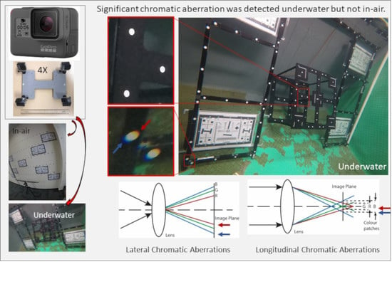
There are two types of CA: longitudinal and lateral or transverse [6]. Longitudinal aberration is measured in the direction parallel to the optical axis. The variation of the principal distance is caused because short wavelengths (i.e., blue) are more strongly refracted by a positive lens and hence, come into focus closer to the lens. On the other hand, a longer wavelength (red) focused further from the lens (Figure 1, left). Lateral aberration is measured perpendicular to the optical axis and is caused by the dispersion of light by the lens system. Therefore, lateral aberrations are also called chromatic differences of magnification or colour misalignment (Figure 1, right). Most lenses are designed to capture images in-air and the effects of chromatic aberrations are minimised using achromatic elements in the lens design [6].
CA can be modeled by different principal distances and radial lens distortion parameters for each colour using the camera calibration method based on [8,9]. This is the method which will be used in this paper. However, it must be mentioned that the modelling and correction of CA is approached differently in various fields. For example, the correction of CA in dermoscopes is considered using a second order radial distortion model of artificial white centroids placed in the field of view of the camera and extracted from the image [12], video processing using an aberration-tolerant demosaicking algorithm [13], color plane warping [14] and light propagation modeling using stereo-camera systems [15].
Several researchers have pointed out that the camera parameters and the accuracy that can be derived processing underwater images can be different from the parameters and accuracy that can be derived by processing images captured in the air. However, while the processing of images underwater can be more challenging [16], it does not mean that the accuracy which can be achieved has to be worse [17].
As mentioned, due to the design of the lens system, there is usually no need to apply colour corrections and chromatic aberrations for short distances in the environment for which the camera system/lenses were designed. Camera systems are usually optimised for in-air operation. The change from air to underwater and, therefore, the different absorption and refraction effects of water may require the introduction of additional correction or modelling if no further considerations are made about the distortion characteristics of the specific camera in combination with the used port (flat or dome port) [18].
In [19], the need to correct or model refraction effects in underwater environments is discussed, pointing out that by far the most common approach is to correct the refraction effect using absorption by the physical calibration parameters. The primary effect can be absorbed by the radial lens distortion parameters. Small, asymmetric effects caused by alignment errors between the optical axis and the housing port (secondary effects) may also exist and can be absorbed as decentering lens distortion parameters.
The aim of this paper was to investigate chromatic aberration effects in low-cost camera systems (several GoPro cameras) calibrated and operated in an underwater environment. The paper will compare the camera parameters of the same cameras operated in-air and underwater as well as investigate the effect of adjustment constraints to the underwater processed images. The reliability and the accuracy of the photogrammetric processed underwater images will be also investigated.
The paper is structured as follows. In the next section, publications that focus on the comparison of camera calibration parameters for in-air and underwater operation and CA will be reviewed. Then, the methodology used for data processing is introduced followed by the introduction of the datasets used in this paper. Then, the results of the different comparison are presented and discussed. The paper will close with a conclusion.
2. Related Work
The number of publications focusing on the direct comparison of camera parameters and performance for in-air and underwater applications is limited. One example of validating the performance of a camera system in both environments has been published by [17]. The focus of this research was on image-based motion analysis as a function of different camera setups and camera settings including the acquisition frequency, the image resolution and the field of view. The authors used GoProHero3+ operated in-air (laboratory) and underwater (swimming pool) to evaluate the three-dimensional (3D) accuracy achievable for the image-based motion analysis. Statistically, the 3D accuracy obtained in-air was poorer than the accuracy achieved in the underwater environment across all the tested camera configurations. However, a conclusion of how the camera parameters are affected by the change of the environment from in-air to underwater was not provided.
In [20], it is reported that the very high accuracy and precision using GoPros underwater is possible. Using multiple GoPro cameras in different test sets, the paper further validated that the consistency of the interior orientation parameters is stable. However, the paper did not investigate CA or provide a comparison of the results achievable underwater and in air.
In contrast, several other authors include CA in their investigations. For instance, [21,22] report CA in fisheye lens systems. In [22], the focus is on the in-air calibration of two lenses and it is interesting to note that this paper found that the aperture affects the magnitude of the CA. However, a systematic influence between the two different lens systems on CA in the different colour bands could not be observed.
In [23], the presence of CA in underwater imagery is reported, which was captured with a camera system coupled with a planar housing port. This paper further investigated the accuracy assessment of dome and planar housings on a distance observation. The dome housing produced results fifty times better than the those from the planar housing.
The authors in [11,23] report CA in underwater imagery. Significant corrections for the radial and decentering distortion parameters indicating lateral CA were observed in images taken from a GoPro Hero Black 3 [11]. A significant trend of different principal distances’ indication longitudinal CA was not observed. In [11], the authors reported in addition that the found lateral CA did not confirm the theory presented in Figure 1. Possible reasons were that the calibration frame only covered 1/3 of the camera’s field of view.
At least two options exist for mitigating errors due to CA [24]: modelling the effect with colour-dependent calibration parameters and correction by image pre-processing. One approach for modelling CA is based on the self-calibrating bundle adjustment [25]. In [26], the self-calibration approach is investigated using a bundle adjustment for cameras of a Ladybug system in-air as well as several GoPro cameras underwater. In contrast to previous works, the application of different constraints was specifically investigated. Overall, four different adjustments per camera were performed, and their results were evaluated especially focusing on CA. The first adjustment did not introduce any constraints, so all colour bands were adjusted independently. The second adjustment considered the constraint that the points of the calibration field have the same coordinates in object space. Building on the second adjustment, the third adjustment added constraints to force the red, green and blue exterior orientation parameters to be equal. The final adjustment used the constraint of the second adjustment as well as the constraints to enforce the equivalence of the principal point coordinates of the cameras corresponding to the three spectral bands. The third adjustment used by [26] is comparable to the adjustment used by [25,26], who concluded that ether common object points or alternatively, common object points with EOP constraints are needed.
Modelling approaches like those of [27] only report limited results. The main conclusion of this paper was that the CA can be expressed by a cubic function of the radial distance from an image frame center. This method corrects CA satisfactorily enough in many cases.
In [28], an underwater measurement of coral reefs with GoPro cameras was performed. Instead of using a bundle adjustment approach in which individual colour images are calibrated, a relative CA correction was performed: two channels are corrected relative to the third. More specifically, the red and blue channels were aligned to the green channel. In a first step, the displacements between the bands is estimated using optical flow. Then, the parameters modelling the displacement are estimated. For this step, two models are investigated—the Brown model using three radial distortion parameters, two decentering distortion parameters and the principal point offset, and a least-squares collocation method. After the displacement parameters are approximated, the blue and red channels are corrected and shifted to the green channel. The deterministic part of the CA is modeled as a second-order polynomial. Though not stated, the collocation approach assumes that the CA is a stationary random process. Furthermore, Gaussian covariance function is used. The paper concludes the collocation performed better overall.
To summarise, existing papers compared the in-air and underwater performances of the same camera but did not analyse the CA. Publications related to CA used different cameras for underwater and in-air calibration and were mainly focused on ether modelling the shift between different bands or investigating in different adjustment models and their constraints. Other aspects covered are the dependencies of the CA on aperture and the comparison of accuracy using different housings.
The contributions of this paper include the comparison of in-air and underwater camera calibration parameters of the same cameras with a specific focus on quantifying any CA. Furthermore, the effectiveness of the various constraints on the EOP is investigated for both in-air and underwater images captured by the same cameras. Moreover, the repeatability of the calculated camera calibration parameters in the underwater environment is investigated. Finally, an experiment designed to replicate a real-world, underwater application using imagery is reported. The effect of CA is analysed by quantifying 3D reconstruction accuracy in terms of spatial distances.
3. Methodology
In this paper, a similar method to [25,26] is used. In this section, the functional model and the add adjustment constraints will be introduced.
3.1. Functional Model
As outlined in the Introduction, the collinearity condition is assumed, i.e., an object point i (X, Y, Z), its homologous image point (x, y)i in image j and the perspective centre of image j (Xc, Yc, Zc) lie on a straight line in a three-dimensional space. All light rays entering the lens system form a bundle passing through the perspective centre. In this paper, images are split into separate red (R), green (G) and blue (B) images. Independent image point measurements are made in each spectral band image. For each spectral band k ϵ {B, G, R}, the collinearity equations are given by
where , are the image point residuals, xp, yp are the coordinates of the principal point offset, c is the principal distance and Δx, Δy are the additive correction terms. Furthermore, (U, V, W) are formulated as
where M is the matrix used for the rotation from object space to image space that can be parameterised as
and ω, ϕ and κ, are the rotation angles around the X, Y and Z axes, respectively. The (Δx, Δy) terms are corrections required to account for non-collinearity due to lens distortion, including CA.
Radial lens distortion is a systematic error source inherent to all lens systems. Out of all systematic errors, the radial lens distortion usually has the largest magnitude, which leads to symmetric image point displacement around the principal point. This displacement can be either towards the principal point (barrel distortion) or away from the principal point (pincushion distortion). In air, wide-angle and fisheye lenses usually have a very strong barrel distortion leading to a very large displacement of points.
In this paper, the functional model for the radial lens distortion is an odd-powered polynomial that models the radial displacement Δrk as follows:
where r is the distance of the image point from the principal point. In general, five parameters were used to model the radial lens distortions for the in-air calibration. Though the number of terms is higher than the normal three, this model has been successfully applied to other wide-angle-lens cameras without compromising object space reconstruction accuracy [29]. For the underwater calibrations reported herein, the 4th and 5th radial lens distortion parameters were not significant, so only three parameters were used. The displacement in x and y can be calculated with
Any lateral CA existing in a camera is predicted to be visible as differing radial displacements in the imagery for the different spectral bands. Any longitudinal CA that exists will be realised as different principal distances for the different colour bands.
In addition to radial lens distortion, there often is decentering distortion. As pointed out by [19] alignment errors between the optical axis and housing port can be absorbed as decentering lens distortion parameters. This distortion is asymmetric about the principal point and is normally much smaller in magnitude compared to the radial lens distortion. Decentering distortions can be modeled using two parameters p1 and p2 per spectral band:
Note that the i and j subscripts have been dropped for clarity reasons from the radial lens distortion function as well as all further distortion functions.
3.2. Least-Squares Adjustments and Constraints
The parametric (or Gauss–Markov) adjustment model was used for the self-calibration. All IOPs are modelled as network invariants. Datum definition was with inner constraints on object points. All unknowns (EOPs, IOPs and object points) were estimated simultaneously. Constraints added to the solution were implemented as weighted constraints according to the unified approach to least squares [30].
Three different least-squares solutions were implemented, which are introduced in Table 1. The first adjustment type, referred to be the independent adjustment (IDP), performs a self-calibration of all colour bands separately. No constraints are added to this adjustment.
Each of the two additional adjustments included object space constraints. The combined adjustment (CMB) constrains that the locations of object points observed in each band are the same. In this adjustment three sets of IOPs (one per colour band) are estimated for each camera. Separate EOPs are estimated for each colour band image.
Finally, the EOPs of each spectral band for a given image are constrained to be equal. These constraints are added to the common object points constraint (EPC) adjustment, which is denoted as EPC. The EPC adjustment forces the red, green and blue EOPs to be equal. This constraint is formulated the way that the base vector (bx, by, bz) between the two bands is assumed to be equal to zero. For instance, the constraint between the red and green band positions can be formulated as
A similar equation is used to enforce the equivalent base vector components between the red and blue images. The relative angles between the pairs of images are also constrained:
where the Δm elements are extracted from the relative rotation matrix, shown here for the blue and green images.
The EOP constraints were enforced with high weights for each of the two groups of constraints: perspective centre position and relative angles. The standard deviations were 0.002 mm and 0.0002°, respectively.
Note that for the in-air calibration, strong fisheye lens distortions are expected [31] and as a result, a fisheye camera model [32] may be more appropriate to use for the in-air calibration. Nevertheless, strong distortions are unlikely for the underwater calibration with a planar port [18,23]. As the collinearity can be used to account for the high distortion by introducing additional polynomial radial lens distortion parameters [32], the collinearity models as introduced above have been used for all adjustments performed as part of this publication.
4. Datasets
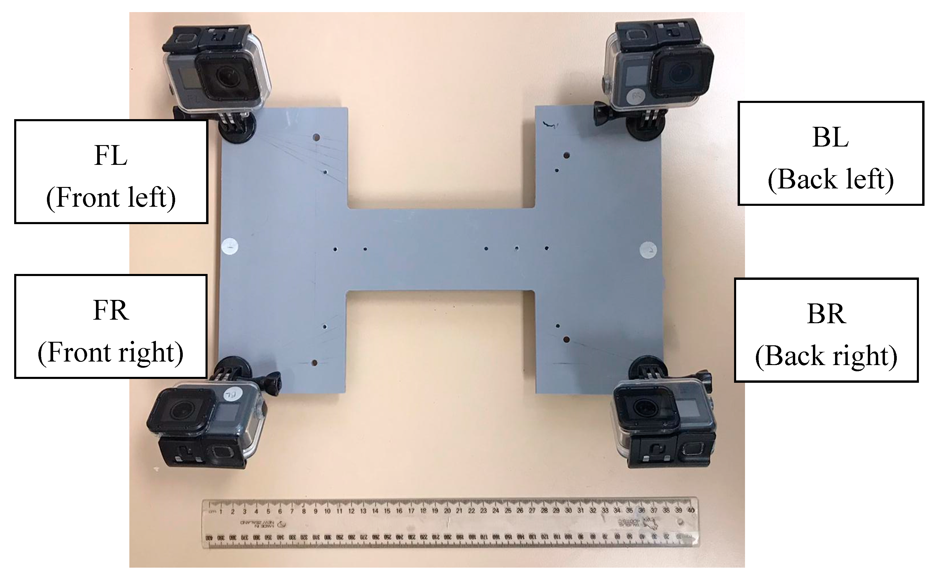
Four GoPro Hero 5 Black cameras (1/2.3″ CMOS; 1.53 µm pixel spacing; 4000 × 3000 pixel captured image size; 2.68 mm nominal focal length) were used to investigate the CA and its effects. The cameras were installed on a frame that can be mounted on a remotely operated vehicle (ROV) (Figure 2). Accordingly, the cameras are labeled Front and Back as well as Left and Right. For instance, BL means the left back camera. Each camera is placed in a water-tight acrylic housing with planar port and mounted on the previously mentioned frame prior to performing the data capture.
For the underwater as well as in-air calibrations, the GoPro cameras were set to wide-angle mode and time-lapse photo acquisition mode. The image capture is synchronised using a remote control triggering to start the camera at the same time. Small time delays during the data capture are negligible for our tests. The cameras were not stopped or paused when moving from the underwater calibration field to the in-air calibration field, aiming to keep the relative positions of the cameras to each other constant. Unfortunately, the frame mount was not as rigid as required for constraining the relative orientation stability of the cameras [26].
The cameras stayed sealed in their housings during the image capture. The underwater and in-air images were captured in quick succession without altering the camera-housing setups in any way. Therefore, following the suggestion from [19], the cameras in their housings are seen as one “unit”.
The cameras were moved around each of the calibration frames whilst maintaining a constant standoff distance. The movement was performed through 120° about the target array for the underwater dataset and about 130° for the in-air dataset. The entire assembly was also rotated by 90° to provide roll diversity. In addition, every effort was made to fill the entire format with targets. These measures provided good geometry for the self-calibration adjustments. Many images of the calibration frames were taken for each calibration sequence. Some images suffered from motion blur and were excluded from any further analysis. An overview of the number of images used in the adjustments is provided in Table 2 and Table 3.
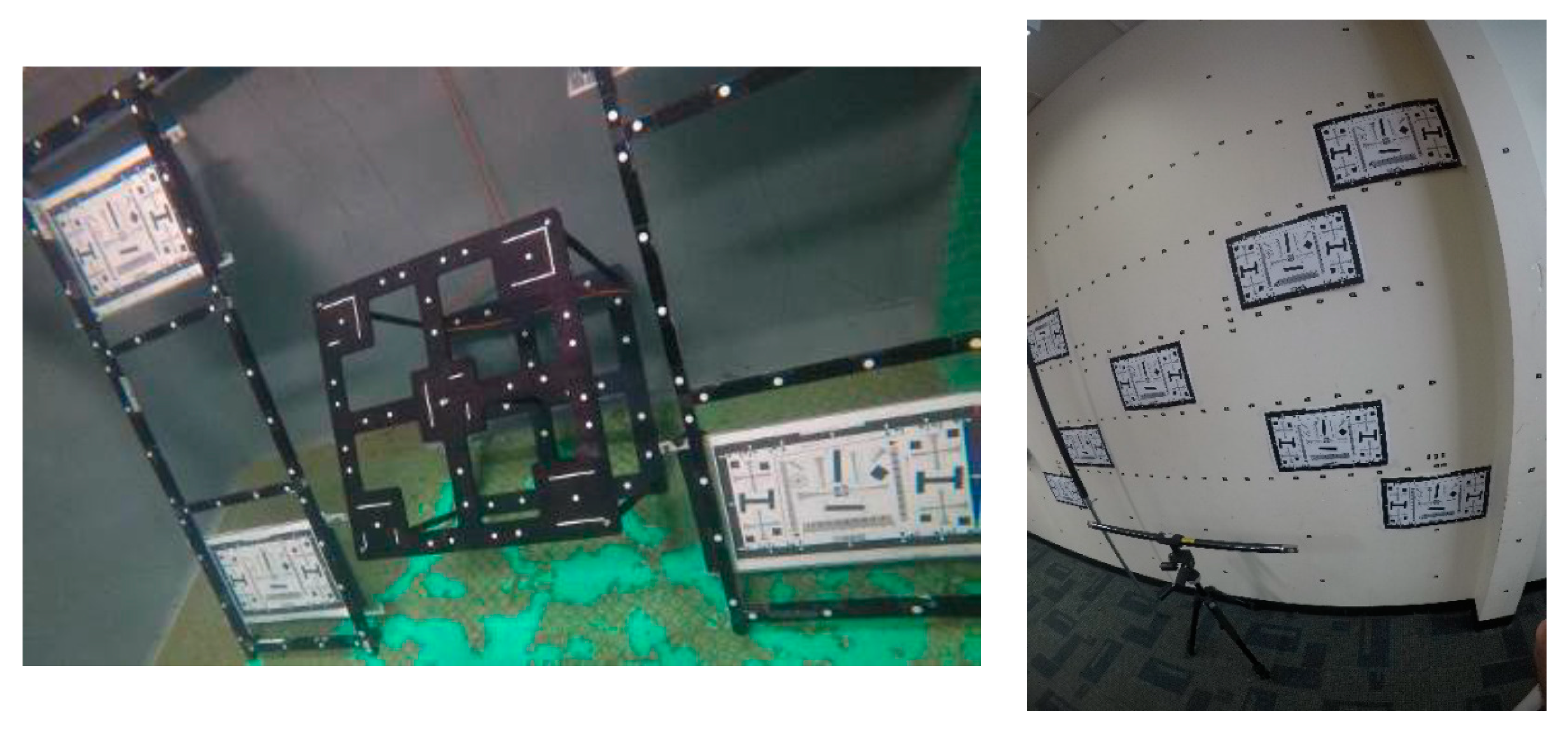
For the underwater images, the cameras mounted in the frame were submerged in a freshwater tank containing a target array. The calibration frame comprising 133 white targets (5 mm diameter) on a black background and is identically with the underwater calibration frame used by [26] (Figure 3, left). The distance between the camera stations and the frame was approximately 1.5 m.
The field of view of the camera is reduced considerably underwater due to the introduction of the planar port. As a result, it was not possible to use the same target field for the underwater and in-air calibrations. To ensure that control points covering the whole image, a larger in-air calibration field was utilised. Two poles and a scale bar placed in front of a wall ensured that the calibration field was not planar (Figure 3, right). The calibration field comprises approximately 155 retro-reflective, circular targets (5 mm diameter). The distance between the camera stations and the calibration field was approximately 2 m during the data capture.
For each camera (FL, FR, BL, BR) three repeats were captured in both environments (underwater (W) and in-air (A)); i.e., FL-A, FR-A, BL-A, BR-A, FL-W, FR-W, BL-W, BR-W. For the data processing, all three repeats of FL-W(1-3) and BL-A(1-3) were processed.
Each dataset contained at least 10 images. From each of the datasets, the red, green, and blue bands were extracted, and the image point observations were performed for each image independently applying centroid fitting using the Australis software (version 8.33). The observations of both datasets nearly covered the entire image plane.
Each dataset was processed using the three adjustment models: IDP, CMB and EPC. The adjustment results of the IDP method are presented in Table 2 and Table 3; the results are representative for all other adjustments. Overall, it can be summarised that the number of object points (ground control points) have been very high for all tests leading to high redundancies. The Root Mean Square (RMS) value is usually around or just below 1 µm for the in-air calibration which leads to the conclusion that the adjustment could successfully account for the strong fish-eye distortion of the camera. The RMS value for the underwater calibration is usually around or just below 1.5 µm and therefore slightly worse compared to the in-air calibration. Nevertheless, for the underwater calibration, the results show that the calibrations were successful, too.
Maximum correlations between the key parameter groups are summarised in Table 4. The results for the in-air and underwater calibrations are very similar and demonstrate the effectiveness of the network design measures employed for the experiments. High correlations (>0.9) were found between the radial lens distortion coefficients in both media. Such correlations are also reported for the wide-angle Ladybug5 camera [29], which exhibit similar high barrel distortion as the in-air calibration of the GoPros. However, these were found to have no detrimental impact on the independent accuracy assessment, but exclusion of distortion terms did degrade accuracy.
5. Evaluation
In this section, firstly the focus is to compare the IOPs of four cameras in-air and underwater. The analysis includes a comparison of the principal distance, principal point offset, radial and decentering distortion and aims to quantify the CA and the impact of the different medium on the IOPs. Secondly, the effectiveness of various constraints (IDP, CMB, EPC) of a representative camera was investigated covering the same IOP as mentioned previously. Then, the reliability of those IOP parameters of a single camera was investigated comparing the results of three repeats. The aim of this test was to investigate how stable the camera is. These tests were similar to [20], but explicitly evaluated the CA. Finally, an accuracy assessment of distance measurements and the impact of CA on those distance observations was investigated simulating the impact of CA on real world applications.
5.1. Test 1: Comparison of Underwater Calibration vs. In-Air Calibration
Firstly, the calibration parameters and the presence of CA were investigated using all four cameras (BL, BR, FL, FR). The CMB adjustment case was utilised. This Section contains firstly the analysis of the principal distance, followed by the analysis of the principal point offset, the radial lens distortion and the final decentering distortions.
5.1.1. Principal Distance
The results of the different principal distances are shown in Figure 4 and Table 5. The first column in Figure 4 shows the results of the four cameras (BL, BR, FL, FR) for the underwater environment. A clear trend is visible that the principal distance of the blue band is always the shortest principal distance, and that the principal distance of the red band is always the longest principal distance. The same observations have been made by [26] and agree with the model in Figure 1 (left) if longitudinal CA is present. The standard deviations of all principal distances are shown in Table 5. The statistical significance of the differences between the principal distances of the different bands was tested. The red–green and red–blue estimates’ differences were normalised by the standard deviation of the difference at 95%. Five of the eight principal distance pairs from the CMB adjustment were significant. It can be concluded that the longitudinal CA is present in the underwater images.
In contrast, the right column in Figure 4 shows the principal distances of the adjustments based on the in-air images taken from the four different cameras. The principal distances for the different bands for each camera are often identical. Statistical testing revealed that only one of the eight principal distance pairs were significantly different from the CMB adjustments. Therefore, the conclusion is that no longitudinal CA is present in the in-air datasets.
To summarise, the same cameras that show the effect of longitudinal CA in the underwater imagery showed no longitudinal CA in the in-air imagery. Noting that both (the in-air and underwater) datasets were captured with the presences of the plane port, hence, the change from air to water influences the behaviour of the light of rays causing CA in one medium but not the other. Consequently, the medium is the main contributing factor for the presence of longitudinal CA in the images.
5.1.2. Principal Point Offset
Then, the location of the principal points was investigated; the results of the calibrations are presented in Figure 5 and Table 6. Again, the left column of the Figure shows the results of the four cameras in the underwater environment. The colour of the dots indicates the band to which the observation belongs. The variation of the principal point location is approximately 3 µm in all cases. The standard deviations of all principal point offsets are shown in Table 6. Only three of the 16 principal point coordinates were statistically different at the 95% confidence level.
The right column of Figure 5 shows the results of the in-air calibrations. Compared to the underwater calibration, the locations of the principal points are more tightly clustered, within approximately 1 μm for all cases. None of the differences are statistically different. A trend indicating the largest offset based on the band is not visible. No final conclusion about the principal point offsets and any correlation to existing CA can be made.
5.1.3. Radial Lens Distortion
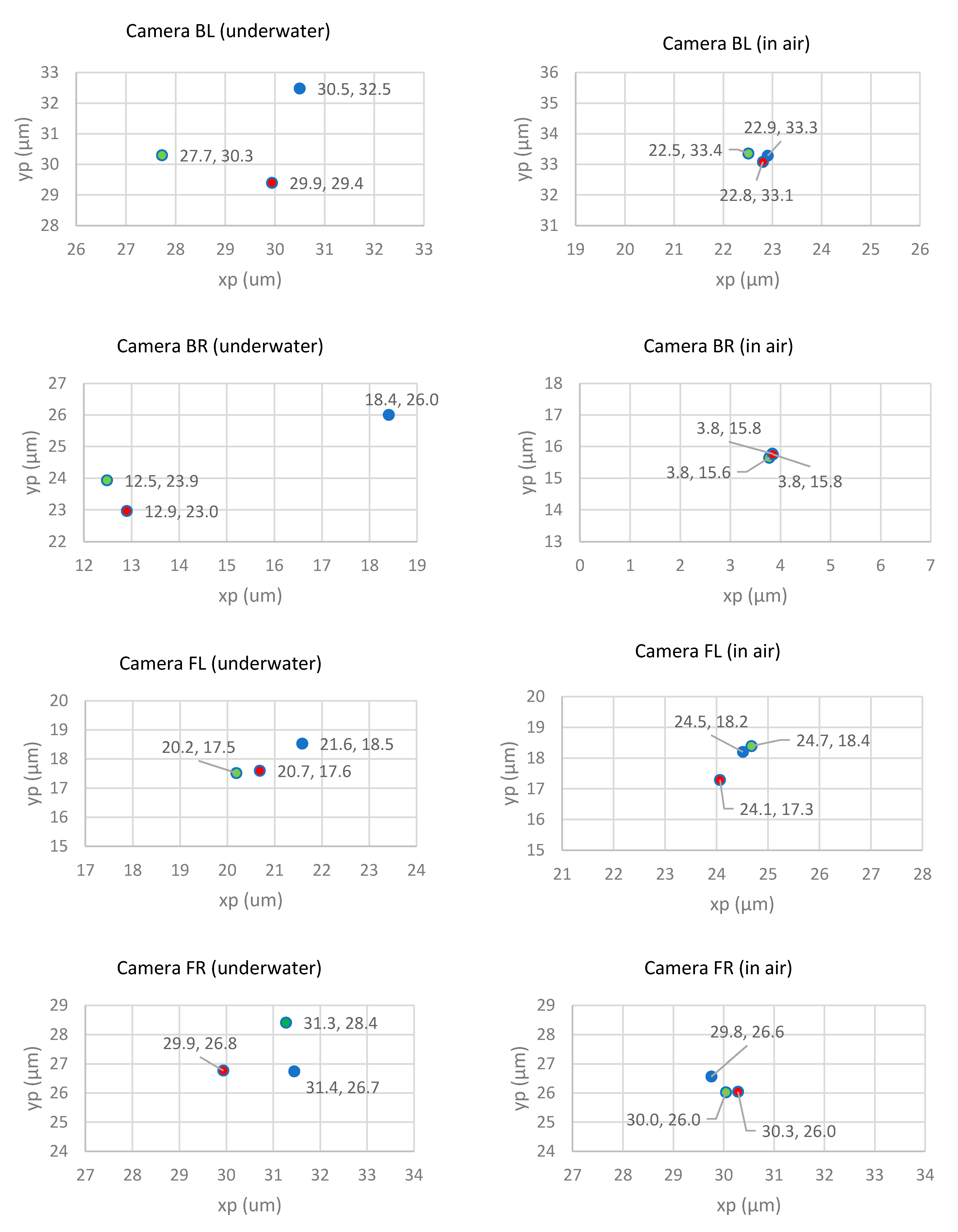
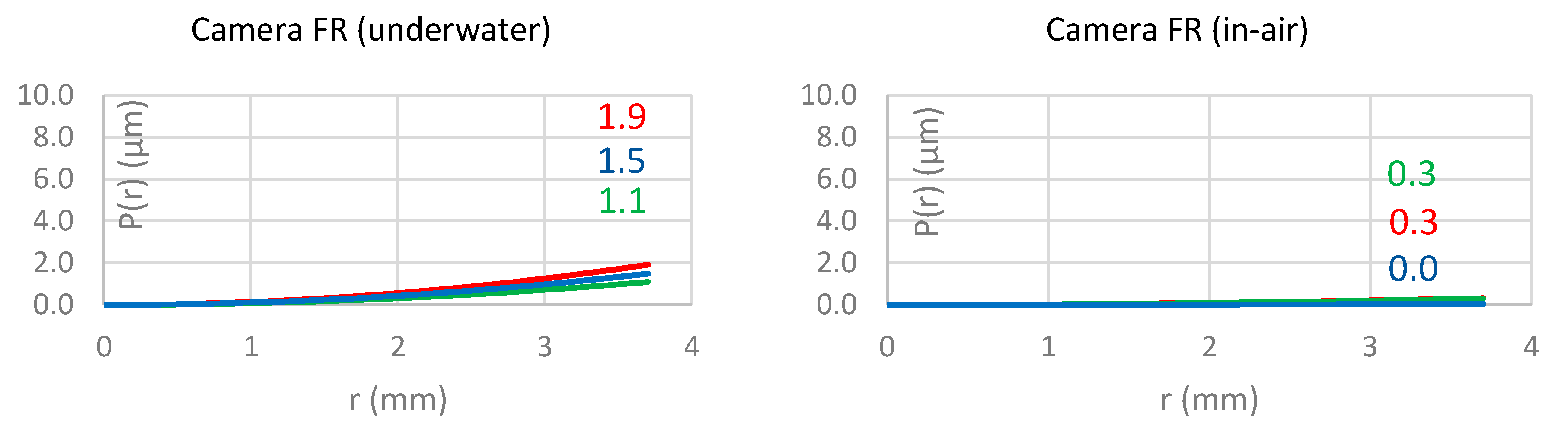
The analysis of the radial lens distortions can be used to investigate any lateral CA which is indicated by large differences in the displacements between the bands. The underwater calibration results (Figure 6, left column) show overall relatively small magnitudes of distortion but with significant differences between the bands. Red has always the smallest radial displacement while blue has the largest displacement. This agrees with the expectations shown in Figure 1 and with the observations made by [26]. The differences between the displacements of the colour bands indicates significant lateral CA. Indeed, this lateral CA is so strong that it is even possible to be seen in the images. Figure 7 show clearly shows that red has the smallest displacement and is oriented towards the centre of the image. In contrast, blue has the largest displacement and the direction is away from the image centre. In contrast, the right image in Figure 7 shows points located at the centre of the image, and no CA is visible for those points.
The in-air calibration results (Figure 6, right column) show very large radial lens distortions with magnitudes a thousand times bigger than in the underwater environment. The large displacements are due to the fisheye lens effect of the cameras in air, which disappears when placing the cameras underwater. Even when accounting for the different scales from in-air and underwater due to the different field of views (FoV) of the same camera in the different environments, the displacements in-air are still very large. The vertical line in Figure 6 (right column) indicates the influence of the different scales; the values show in italics next to the line indicate the displacement values of this distance. However, even though the displacements are large, significant differences between the different bands are not visible. It must be highlighted that the optics of the cameras were unchanged between the underwater and in-air image captures. Hence, it can be concluded that there is no lateral CA present in the in-air imagery.
To summarise, the same cameras which show the effect of lateral CA in the underwater imagery show no lateral CA in the in-air imagery. Hence, similar to the conclusion made for the longitudinal CA, the change from air to water influences the behaviour of the light of rays causing CA in one medium but not the other. Consequently, the medium is a main contributing factor for the presence of longitudinal CA in the images of the investigated cameras.
5.1.4. Decentering Distortion
Finally, Figure 8 presents the results of the decentering distortion parameters. The displacements are very small in magnitude for the underwater environment (left column) as well as for the in-air environment (right column). The differences between the different bands are not significant and no systematic trend can be observed with regards to which bands have the largest displacement.
5.1.5. Conclusions
The conclusion is that while significant lateral and longitudinal CA can be observed for the underwater datasets of different cameras, no CA was found in the in-air images of the same cameras. A separate analysis of the impact of the flat port housing vs. no housing vs. dome port housing is not included. For details about the effect of different housings (flat port and dome ports) in an underwater environment, we referred to [18,23]. As the housing was unchanged, the change from air to water influences is the main source for the changing of the behaviour of the light of the rays causing CA in one medium but not the other. Consequently, the medium is a main contributing factor for the presence of longitudinal CA in the images.
5.2. Test 2: Underwater: Effectiveness of the Various Constraints on the EOPs
The second test investigates the effectiveness of various adjustment constraints. As CA could only be observed in the underwater images, this Section only presents the results of one of the cameras (camera BL) for the underwater environment. However, any other cameras could have been used as the results of all cameras are very similar and show the same trends.
5.2.1. Principal Distance and Point Offset
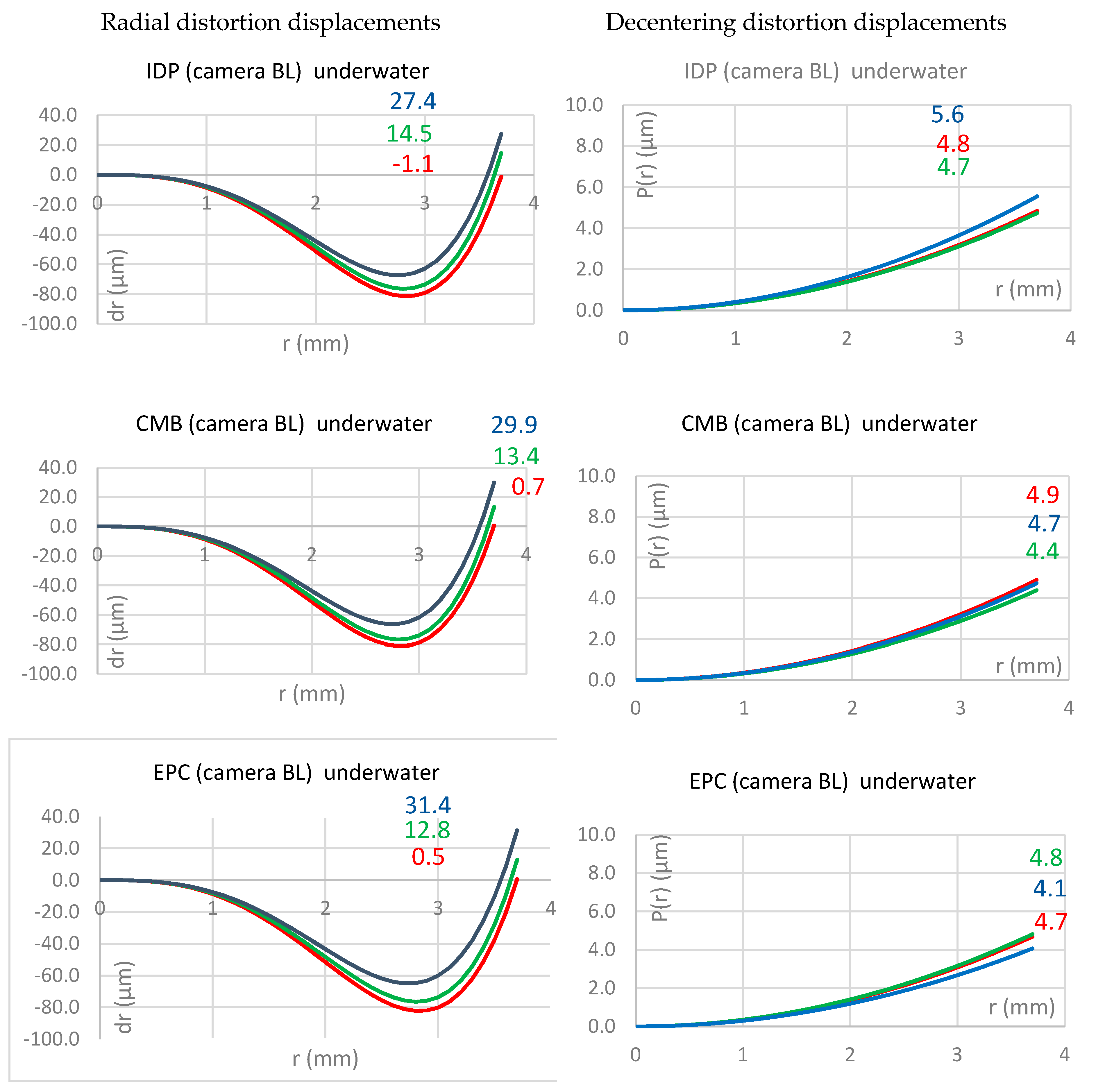
Figure 9 shows the results for the principal distance (left column) and principal point location (right column). The first row presents the results of the IDP adjustment, followed by the results of the CMB adjustment in row two and the EPC adjustment in the third row. The IDP as well as the CMB adjustment show the trend that the principal distance of the blue band is the shortest, followed by green and red. While the explicit standard deviations of the principal distances and offsets are not presented, the precision of the IOPs from the IDP adjustments was an average of 46% lower (i.e., worse) than that of the CMB adjustments. Four of the eight principal distance pairs from the IDP adjustment were found to be statistically different at the 95% confidence level. Five of the eight principal distance pairs from the CMB adjustment were significant. As previously mentioned, this agrees with the findings in [26] as well as with Figure 1. The EPC adjustment, which forces the EOP parameters to be identical, breaking from the trend. Here, red has the shortest principal distance followed by blue and green. Three of the principal distance pairs from the EPC adjustment were significantly different. It can be concluded the longitudinal CA is present in the underwater images when applying the IDP, CMB and EPC adjustment constraints.
Focusing on the principal point locations, there is a systematic trend visible for this specific camera. The location of the principal point of the blue band is always furthest away from the origin of the image coordinate system, and that the green band’s is closest to the origin of the image coordinate system. Adding the constraints forces the principal points to be closer to each other. The differences in the principal point locations in the IDP adjustment are approximately 3 μm in the x direction and approximately 18 μm in the y direction. Four of the differences are significantly different. The location difference is reduced to approximately 2 μm in the x direction and approximately 2 μm in the y direction in the CMB adjustment. Only three of the 16 principal point coordinates were statistically different at the 95% confidence level. The differences of the principal point locations is even smaller (~0.1 μm) for the EPC adjustment. None from the EPC adjustment are significantly different.
5.2.2. Distortions
Figure 10 shows the results for the radial (left column) and the decentering lens distortion displacement (right column). For all adjustment types, the smallest radial distortion can be observed by the red band, followed by the green and blue bands. The difference in the displacement from red to green is approximately 13 µm and the displacement from green to blue is slightly larger with approximately 13 to 19 µm. The same trend is visible in all three adjustment results and indicates significant lateral CA. Overall, the different adjustment constraints do not influence the radial lens distortion profiles.
The magnitude of the decentering distortion is much smaller and always stays nearly under 5 µm and therefore, is marginal compared to the radial lens distortion. Again, the different constraints do not impact the results significantly.
5.2.3. Conclusions
The EPC constraint adjustment forces the principal distance and the principal point offset to be similar and indicate no longitudinal CA. In contrast, the IDP and CMB adjustments suggest the existence of longitudinal CA. The change in the adjustment constraints has no significant influences on the radial or decentering distortions, indicating the presence of lateral CA for all adjustments.
5.3. Test 3: Repeatability of Interorior Orientation Parameters (IOPs)
The aim of the third test is to investigate if the IOPs are repeatable. In other words, is the camera stable and can the CA influence be reproduced? As test one did not find any significant differences in the behaviours of the four tested cameras, only the camera FL for the underwater repeat sets and the camera BL for the in-air repeat were used for this test. Based on the results presented in test 2, the CMB adjustment results are presented in this Section only. As shown in test 2, the main difference between the CMB and EPC adjustment results are that the results of the principal distances and the principal point offset of the different bands are more homogenous. However, the distortion parameters for the CMB and EPC adjustment are comparable.
5.3.1. Principal Distance
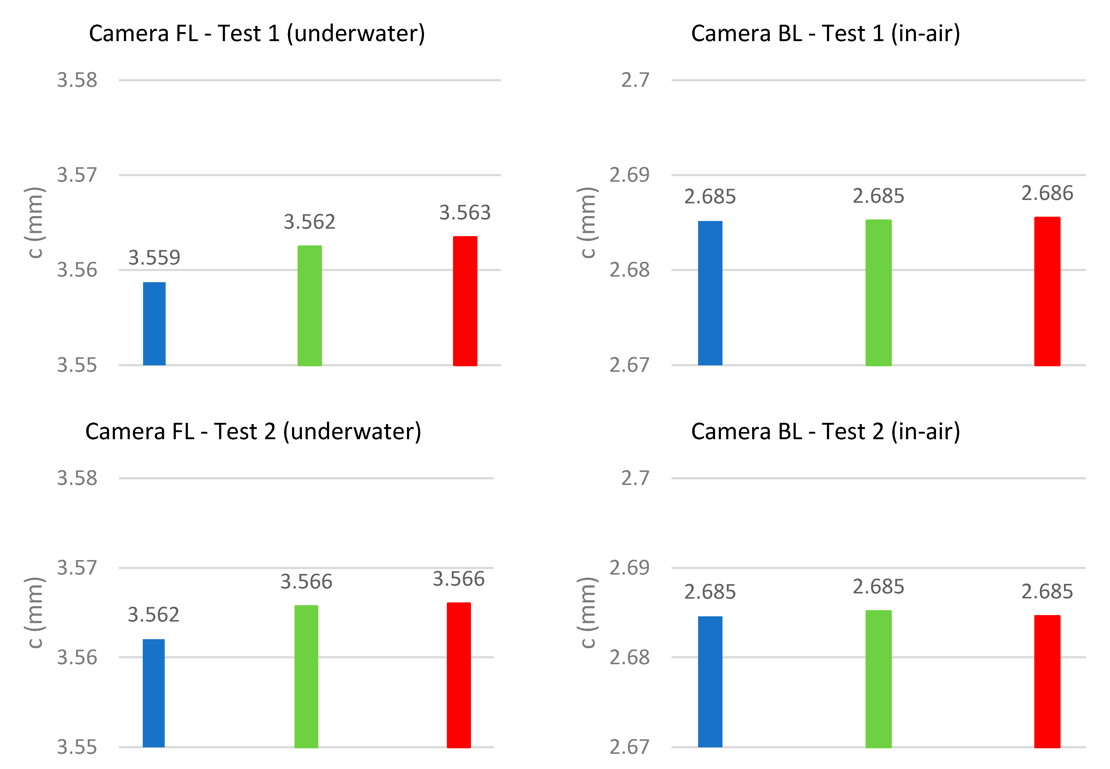
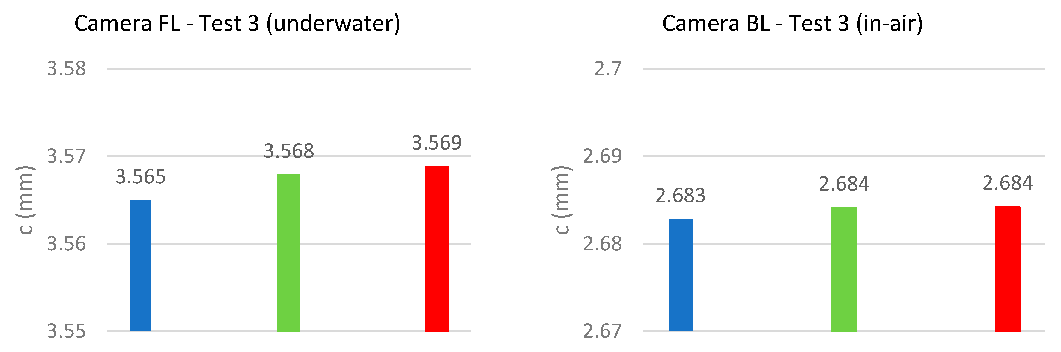
Figure 11 presents the results of the repeats of the FL camera underwater (left column) and the BL camera in-air (right column). From the three repeats, two sets of parameter differences can be evaluated for each band for significance at the 95% confidence level. Four of the six pairs of principal distances were significantly different from the underwater calibrations, while only one was different for the in-air calibrations. While the differences between the bands seem to be very stable for each of the repeats of the underwater dataset, the actual principal distances vary between the repeats, indicating a less stable camera IOP. This does not agree with the results found in [20] with an older version of the camera (GoPro 3).
The results produced for the in-air dataset are very similar between the different repeats showing no significant differences and therefore indicating a very stable camera. CA is not visible in the in-air dataset.
5.3.2. Principal Point Offset
The comparison of the location of the principal point offsets for three repeats are presented in Figure 12. The left column presents the underwater repeats and the right column presents the in-air results.
The underwater repeats show again (similar to test 1 and 2) that the location of the principal point of the blue band is furthest from the image coordinate origin while the location of the principal point of the green band is again closest to the image coordinate origin. While the relative distances between the locations of the principal points are comparable and no more than 3 μm apart, the differences in the absolute location of the principal point are significant. Five sets of principal point coordinates were significantly different from the underwater datasets. This behaviour was not observed by [20], who used a previous version of a GoPro camera (series 3). The absolute locations of the principal point in-air appear to be more stable and are more tightly clustered, with differences of less than 1 μm. However, seven sets were significantly different from the in-air calibrations.
5.3.3. Radial Lens Distortion
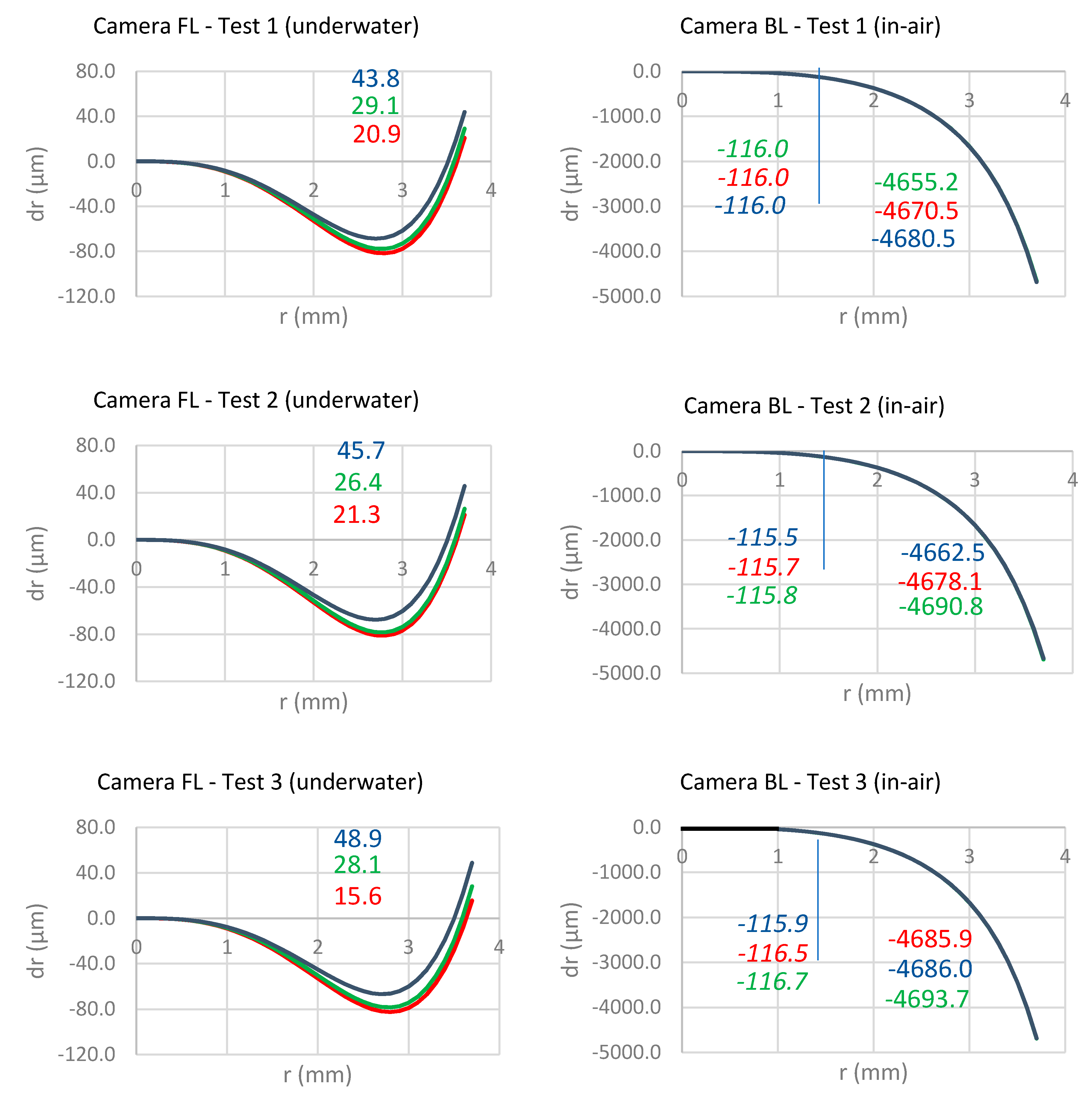
Figure 13 summarises the results of the underwater (left column) and in-air (right column) adjustments of three repeats with regard to the radial lens distortion parameters. As previously discussed, the underwater images show a lateral CA expressed by the large differences in the radial displacements between the different bands. The displacements of the blue band at the edge of the image are nearly twice that of the magnitude of the red band. The displacement results between the different repeats is stable for the underwater calibration.
Then, the magnitudes of the displacements are much smaller for the underwater environment (the maximum displacement is smaller than 50 μm) compared to the displacement in-air (maximum displacement is just below 4700 μm). The vertical line in Figure 13 (right column) indicates the influence of the different scales; the italic values next to the line indicates the displacement values when accounting for the different scale due to the change in medium. Even when accounting for the different scales, the displacements in-air are still large (more than 110 μm). However, even though the displacements are large, significant differences between the different bands are not visible. Therefore, no lateral CA or even a trend for which band has the smallest or largest displacement is visible in the in-air datasets.
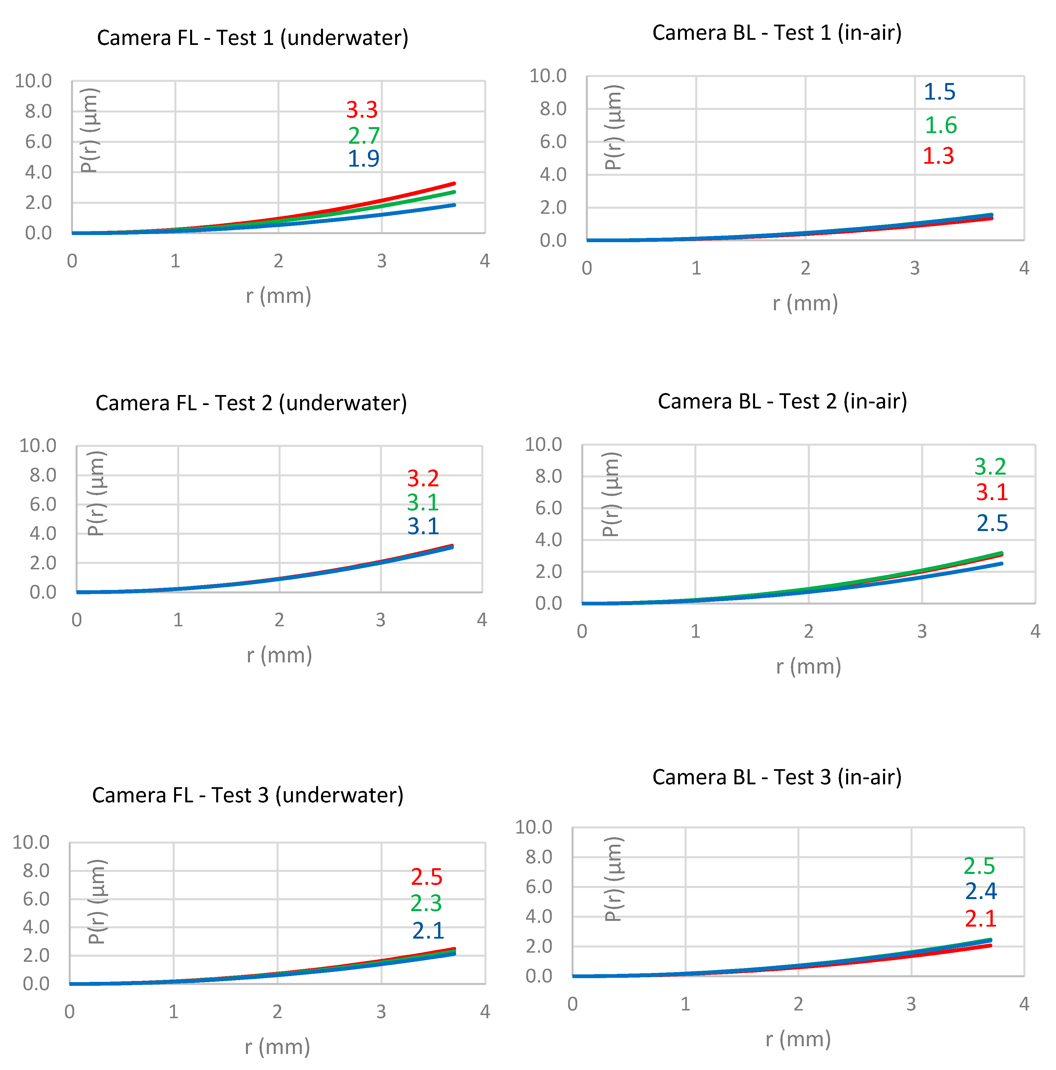
5.3.4. Decentering Distortion
Figure 14 presents the results of the decentering distortions for the underwater environment (left column) and in-air environment (right column). The same observations made for the radial distortion can be made for the decentering distortions. Regarding the underwater environment, this means that the same bands always show the smallest (blue) and largest (red) displacements and that the magnitude of the displacement is small and comparable (no significant difference). Regarding the in-air calibration, this means that there is no systematic trend of which band shows the largest displacements. However, compared to the radial displacements for the in-air calibration, the magnitude of the decentering displacement is very small.
5.3.5. Conclusions
The principal distances and the principal point offsets of the underwater repeats show significant differences. While the values are significantly different for each band between the repeats, the relative differences between the bands seems similar. The average RMS value for the image point positioning underwater is 1.6 µm for the CMB adjustment (and 1.7 µm for the EPC adjustment). In contrast, the principal distances and the principal point offsets in-air seem to be very stable. The average RMS value for the image point positioning in-air is 0.9 µm for the CMB adjustment (and 1.0 µm for the EPC adjustment). The radial and decentering lens distortion displacements are very similar for each repeat and appear stable both underwater and in-air.
As the same cameras are used in the same housings and as the camera settings are unchanged, the differences in the principal distance and the principal point offset in the underwater dataset cannot be caused by changes within the camera but the medium in which the images are taken. Therefore, it can be concluded that there is the requirement of in situ camera calibration for each underwater data capture and a recalibration of the camera for each new dataset captured mainly due to the medium in which the camera is operated (underwater).
Alternatively, it is suggested to use the EPC adjustment. While the radial and decentering lens distortion displacements are similar between the different adjustment types, the EPC adjustment constrains the principal distances and the principal point offsets to be stable. The same conclusion has been made by [26].
5.4. Test 4: Precision and Accuracy Assessment
5.4.1. Precision
Based on the conclusion of test 2, the CMP adjustment was used for investigating the precision of the EOP estimation in this Section. In this adjustment, each spectral band image has a separate set of EOPs and there are no conditions to enforce the fact that they were captured from the same position and in the same orientation. In contrast, the EPC adjustment adds adjustment constraints to force the EOPs of each band to be the same. As a by-product, the principal point coordinates for each spectral band are effectively the same. The common EOP element condition needs to be enforced with constraints, otherwise the EOPs from each band will differ due to random errors and CA. There are 6 constraints per pair of images (three for the relative position and three for the relative angles), six for R-G and six for R-B. Not enforcing these constraints means the camera positions can differ by several millimetres and the angles can differ by several arcminutes.
For each medium (water and air), all the EOP differences are provided for each dataset in Table 7. There is no CA effect in air, so the differences are overall very small and the RMS values are at the same level as the EOP precision. The EOP precision values are presented in Table 8. For instance, the position RMS for all air calibration is 0.1 mm, which is the same value for the precision results. In contrast, the position RMS for the underwater calibrations is between 1.7 and 1.9 mm compared to the precision which has a maximum value of 0.4 mm. The angular values mirror these findings. While this is not an exact comparison since the precision of the differences should be propagated, it is a good indicator for detecting any systematic and significant influences. The in-air RMS values are just due to random error. In contrast, the underwater calibration RMS values are 3x–6x higher than the EOP precision, so these values contain both random error and the systematic effects from the CA.
5.4.2. Accuracy
Then, the accuracy was investigated. For this test, the focus was purely on the underwater datasets. There are three reasons to exclude the in-air images in this test. Firstly, all previous tests have shown that the in-air datasets are not affected by CA whereas the main aim of this paper is to quantify and investigate the influence of CA. Then, the purpose of the system development is for underwater measurement and the in-air tests have been mainly used to better understand the impact of the IOP when changing the medium from in-air to underwater.
The aim of this test was to simulate a real-world underwater feature pickup of points as is done when surveying shipwrecks or infrastructure. Stereo-photogrammetry is often applied for such surveys, and the cameras are pre-calibrated. The stereo camera set up is ether achieved by mounting the two-camera system into a large housing, or by installing the cameras’ fixed frame. As the installation of our cameras on a frame was not solid enough, the alternative of removing an image pair from each underwater calibration was applied. The remaining images were used to estimate the calibration parameters.
The selected stereo image pair ensured good base separation, but a high convergence angle could not always be achieved due to the calibration set up and the limited space in the water tank. The extracted image pair was used in a separate bundle adjustment using the IO parameters determined with the larger subset of images for the accuracy assessment.
To overcome the datum defect, seven parameters had to be fixed. Two different methods were used to achieve this. Firstly, six EOPs from one image were fixed, plus one distance on the inner frame was included as an observation. The one distance in object space could be a scale bar placed in the field of view of the cameras in a real-world application. We refer to this adjustment as 6EOP in the following descriptions. Alternatively, when using a scale bar, it is common to fix the distance between the cameras. Therefore, the second method holds six EOPs from one image fixed plus one base vector component from a second image is fixed (similar to a dependent relative orientation). This simulates a stereo-camera, which is also often used in real-world applications. We refer to this adjustment as 7EOP in the following descriptions. For each method, five bundle adjustments were performed in total as formerly mentioned (for the IDP constraint, three adjustments: B only, R only, R only, then one adjustment using the CMB and one adjustment using the EPC constraint).
Check points were used to assess accuracy. Only targets placed on the rigid, central frame of the calibration field (Figure 2) were used as check points, which were solved as tie points in a second independent bundle adjustment referred to as accuracy assessment bundle adjustment. The tie point coordinates were compared with the reference coordinates to determine the differences, from which the mean, RMS, min and max differences were computed. The mean tie point precision from each case is summarised in Table 9. The CMB adjustment precision is superior to that of the IDP cases by 35% and is the same as for the EPC cases. The 6EOP test precision is superior to the 7EOP precision by 40%.
The results for the 6EOP method are presented in Table 10. The RMS values were derived by comparing known coordinates with those determined by photogrammetry. The number of available check points varied between 4 and 10, but in most cases, 8–10 check points were available. The only case where this was not possible was for the camera FR. Therefore, instead of using data from the camera FW, the second repeat of the camera FL was used. The different repeats are labelled with FL1 and FL2.
The previous tests showed the largest radial displacement due to CA for the blue band followed by the green and red ones. The impact of the CA was also visible in this test as well. The RMS values for the blue band were the largest (up to 13 mm) followed by the red (up to 10.6 mm) and green (up to 7.7 mm) for the cameras BL, BR and FL2. Only FL1 shows a different trend with an inverted order. The CMB adjustment usually produces RMS values as large as the blue band (the largest RMS is 11 mm) again for the cameras BL, BR and FL2 but not for the camera FL1. Only introducing additional constraints (EPC adjustment) improves the RMS values and reduces the largest RMS value to 8.1 mm and the smallest value of less than 1mm. Overall, these RMS values are very high compared to the precision that can be achieved (c.f. Table 9).
The results for the 7EOP method (holding 6EOPs from one image fixed plus one base vector component) are presented in Table 11. Like in the 6EOP method, the largest RMS value is produced by a blue band (up to 17 mm) when using the IDP adjustment method. However, the blue band does not always have the largest value; also, the red band produces a very high RMS, e.g., for camera FL1, up to 11.1 mm. Again, the RMS values of the green band are the smallest (up to 8.1 mm). Overall, the RMS values have increased using the 7EOP method compared to the 6EOP method when using the IDP adjustment, which follows the trend of the tie point precision (Table 9). The RMS values are also increased for the CMB adjustment (largest RMS is 10.5mm) and for the EPC adjustment (largest RMS value is 10.2mm) when using the 7EOP method compared to the 6EOP method.
5.4.3. Conclusions
The analysis of the precision shows that air RMS values are just due to random errors. In contrast, the underwater calibration RMS values are 3x–6x higher than the EOP precision, so these values contain both random error and the systematic effects from the CA. For the accuracy assessment, two method were used. One simulating the use of a scale bar and one simulating a stereo-camera. The scale bar method using the EPC adjustment produces the smallest RMS values, which are, however, significant.
6. Conclusions
The aim of this paper was to investigate the chromatic aberration (CA) effects in low-cost camera systems (several GoPro cameras) operated in an underwater environment. This is an increasingly important field of research thanks to the availability of these cost-efficient camera solutions together with the opportunity to mount them on small ROVs. More precise projects for capturing underwater objects are being undertaken by many different researchers. The most popular fields of underwater image capture with such systems are within the area of coral reef monitoring as well as shipwreck mapping.
The contributions of this paper include the comparison of in-air and underwater camera calibration parameters of the same cameras with a specific focus on quantifying any CA. The comparison of four cameras used for underwater and in-air calibration showed that significant lateral and longitudinal CA can be observed for the underwater datasets. However, no CA was found using the same cameras calibrated in-air. The change from air to water influences the behaviour of the light of rays, causing CA in one medium (water) but not the other (air). Consequently, the medium is a main contributing factor for the presence of CA in the underwater images.
Furthermore, the effectiveness of the various constraints on the EOP is investigated in both in-air and underwater images captured by the same cameras. Three adjustment constraints have been investigated. The IDP method does not add any constraints; all bands are calibrated independently. The CMB constrains the locations of common object points captured by different bands so that they are the same. Finally, the EPC constrains the camera EOPs of the different bands to be the same in addition to the CMB constraint. The EPC constraint adjustment resulted in the principal distance and the principal point offset to be similar and indicated no longitudinal CA. In contrast, the IDP and CMB adjustments suggest the existence of longitudinal CA. There was a clear presence of lateral CA for all adjustments, but the change of the adjustment constraints has no significant influence on the radial or decentering distortions.
Moreover, the repeatability of the calculated camera calibration parameters in the underwater environment was investigated. The principal distances and the principal point offsets of the underwater repeats show significant differences. In contrast, the principal distances and the principal point offsets in-air seem to be very stable. The radial and decentering lens distortion displacements are very similar for each repeat and appear stable—underwater and in air. As the same cameras have been used and as the camera settings were unchanged, the difference in the principal distances and the principal point offsets in the underwater dataset cannot be caused by changes within the camera but the medium in which the images were taken. Therefore, it can be concluded that there is the requirement of in situ camera calibration for each underwater data capture and a recalibration of the camera for each new dataset captured mainly due to the medium in which the camera is operated (underwater). Alternatively, it is suggested to use the EPC adjustment. While the radial and decentering lens distortion displacements are similar between the different adjustment types, the EPC adjustment constrains the principal distances and the principal point offsets to be stable. The same conclusion has been made by [26].
Finally, a precision and accuracy assessment analysing the distance observation underwater was performed by simulating a real-world application using the images and quantifying the effect of CA on these distance observations. The analysis of the precision shows that the RMS values of the in-air adjustment are just due to random error in contrast to the underwater calibration RMS values being 3x–6x higher than the EOP precision. Hence, they contain not only random errors but also systematic effects from the CA. For the accuracy assessment, two methods were used: one simulating the use of a scale bar and one simulating a stereo-camera. The scale bar method using the EPC adjustment produces the smallest RMS values which are, however, significant.
Overall, it can be concluded that the common approach to correct the refraction effect using absorption by the physical calibration parameters will lead to significantly different camera calibration parameters of the same camera in-air and underwater. While effects such as CA are often not present in in-air application due to the cameras being mainly designed to be operated in air, the change of the medium from air to water can introduce significant CA which will not only impact the precision achievable but also the accuracy.
Future work will investigate the CA in the underwater environment. This paper has shown large differences for different repeats for the same camera underwater. There are several possible reasons. One of them is a possible distance dependency. Therefore, a further test will be conducted to quantify the effect of the distance to the calibration frame on the calibration parameters and CA, and if possible, to model this distance dependency. Furthermore, it is best practise to calibrate the cameras in a tank before using it for a possible job, e.g., in ocean water. The influence of the different water qualities on the camera calibration and the CA is another focus of future research.
Author Contributions
P.H. and D.D.L. contributed both to the data capture. The pre-processing of the data was performed by P.H. while the data processing (least square adjustments) have been performed by D.D.L. Both authors have contributed to the analyses and visualisation of the data as well as to the writing of the paper. All authors have read and agreed to the published version of the manuscript.
Funding
The authors would like to acknowledge the financial support of Curtin University’s Faculty for Science and Engineering and the Natural Sciences and Engineering Research Council of Canada (RGPIN-2018-03775).
Acknowledgments
The authors would like to acknowledge Curtin’s Centre for Marine Science and Technology (CMST) for providing access to the tank room and part of the calibration frame and for their help to clean up the floor of the physics building at Curtin after flooding the tank room and the building floor. Cornelius Bothma is thanked for digitising the points of all datasets as part as his fourth-year project. The Australian Research Council by supporting our research about the Photogrammetric Reconstruction for Underwater Virtual Heritage Experiences (ARC LP180100284).
Conflicts of Interest
The authors declare no conflict of interest.
References
- Sultana, S.; Dixit, S. A survey paper on 3D reconstruction of underwater coral reef images. In Proceedings of the IEEE 2017 International Conference on Computing Methodologies and Communication (ICCMC), Erode, India, 18–19 July 2017; pp. 12–15. [Google Scholar]
- Napolitano, R.; Chiariotti, P.; Tomasini, E.P. Preliminary assessment of photogrammetric approach for detailed dimensional and colorimetric reconstruction of Corals in underwater environment. In Proceedings of the 2018 IEEE International Workshop on Metrology for the Sea; Learning to Measure Sea Health Parameters (MetroSea), Bari, Italy, 8–10 October 2018; pp. 39–45. [Google Scholar] [CrossRef]
- Young, G.C.; Dey, S.; Rogers, A.D.; Exton, D. Cost and time-effective method for multi-scale measures of rugosity, fractal dimension, and vector dispersion from coral reef 3D models. PLoS ONE 2017, 12, e0175341. [Google Scholar] [CrossRef] [PubMed]
- Harvey, E.; Bunce, M.; Stat, M.; Saunders, B.; Kinsella, B.; Machuca Suarez, L.; Lepkova, K.; Grice, K.; Coolen, M.; Williams, A.; et al. Science and the sydney. In From Great Depths the Wrecks of HMAS Sydney [II] and HSK Kormoran; UWA Publishing: Perth, Australia; The Western Australian Museum: Perth, Australia, 2016; pp. 279–303. [Google Scholar]
- Fukunaga, A.; Burns, J.H.R.; Pascoe, K.H.; Kosaki, R.K. Associations between benthic cover and habitat metrics obtained from 3D reconstruction of coral reefs at different resolutions. Remote Sens. 2020, 12, 1011. [Google Scholar] [CrossRef] [Green Version]
- ASPRS (American Society of Photogrammetry and Remote Sensing). Manual of Photogrammetry; McGlone, J.C., Ed.; ASPRS: Bethesda, MD, USA, 2004; ISBN 1-57083-071-1. [Google Scholar]
- Brown, D.C. Close range camera calibration. Photogramm. Eng. 1971, 37, 855–866. [Google Scholar]
- Fraser, C.S.; Shortis, M.R.; Ganci, G. Multi-sensor system self-calibration. In Videometrics IV; El-Hakim, S.F., Ed.; SPIE: Bellingham, WA, USA, 1995; Volume 2598, pp. 2–18. [Google Scholar]
- Ziemann, H.; El-Hakim, S.F. On the definition of lens distortion reference data with odd-powered polynomials. Can. Surv. 1983, 37, 135–143. [Google Scholar] [CrossRef]
- Brown, D.C. Decentring distortion calibration. Photogramm. Eng. 1966, 22, 444–462. [Google Scholar]
- Helmholz, P.; Lichti, D.D. Assessment of chromatic aberrations for GoPro 3 cameras in underwater environments. ISPRS Ann. Photogramm. Remote Sens. Spat. Inf. Sci. 2019, 4, 575–582. [Google Scholar] [CrossRef] [Green Version]
- Wighton, P.; Lee, T.K.; Lui, H.; McLean, D.; Atkins, M.S. Chromatic aberration correction: An enhancement to the calibration of low-cost digital dermoscopes. Skin Res. Technol. 2011, 17, 339–347. [Google Scholar] [CrossRef]
- Korneliussen, J.T.; Hirakawa, K. Camera processing with chromatic aberration. IEEE Trans. Image Process. 2014, 23, 4539–4552. [Google Scholar] [CrossRef]
- Rudakova, V.; Monasse, P. Precise Correction of Lateral Chromatic Aberration in Images; Klette, R., Rivera, M., Satoh, S., Eds.; Lecture Notes in Computer Science; Springer: Berlin/Heidelberg, Germany, 2014; Volume 8333, pp. 12–22. [Google Scholar] [CrossRef] [Green Version]
- Skinner, K.A.; Iscar, E.; Johnson-Roberson, M. Automatic Color Correction for 3D Reconstruction of Underwater Scenes. In Proceedings of the 2017 IEEE International Conference on Robotics and Automation (ICRA), Singapore, 29 May–3 June 2017; pp. 5140–5147. [Google Scholar]
- Čejka, J.; Bruno, F.; Skarlatos, D.; Liarokapis, F. Detecting square markers in underwater environments. Remote Sens. 2019, 11, 459. [Google Scholar] [CrossRef] [Green Version]
- Bernardina, G.R.D.; Cerveri, P.; Barros, R.M.L.; Marins, J.C.B.; Silvatti, A.P. In-air versus underwater comparison of 3D reconstruction accuracy using action sport cameras. J. Biomech. 2017, 51, 77–82. [Google Scholar] [CrossRef]
- Menna, F.; Nocerino, E.; Fassi, F.; Remondino, F. Geometric and optic characterization of a hemispherical dome port for underwater photogrammetry. Sensors 2016, 16, 48. [Google Scholar] [CrossRef] [Green Version]
- Shortis, M. Camera Calibration Techniques for Accurate Measurement Underwater. In 3D Recording and Interpretation for Maritime Archaeology; McMarthy, J.K., Benjamin, J., van Duivenvoorde, M., Eds.; Springer: Berlin/Heidelberg, Germany, 2019. [Google Scholar] [CrossRef] [Green Version]
- Helmholz, P.; Long, J.; Munsie, T.; Belton, D. Accuracy assessment of go pro hero 3 (black) camera in underwater environment. Int. Arch. Photogramm. Remote Sens. Spat. Inf. Sci. 2016, 41, 477–483. [Google Scholar] [CrossRef]
- Van den Heuvel, F.; Verwaal, R.; Beers, B. Calibration of fisheye camera systems and the reduction of chromatic aberration. Int. Arch. Photogramm. Remote Sens. Spat. Inf. Sci. 2006, 36, 1–6. [Google Scholar]
- Pöntinen, P. Study on chromatic aberration of two fisheye lenses. Int. Arch. Photogramm. Remote Sens. Spat. Inf. Sci. 2008, 37, 27–32. [Google Scholar]
- Menna, F.; Nocerino, E.; Remondino, F. Flat versus hemispherical dome ports in underwater photogrammetry. Int. Arch. Photogramm. Remote Sens. Spat. Inf. Sci. 2017, 42, 481–487. [Google Scholar] [CrossRef] [Green Version]
- Cronk, S.; Fraser, C.; Hanley, H. Automated metric calibration of colour digital cameras. Photogramm. Rec. 2006, 21, 355–372. [Google Scholar] [CrossRef]
- Luhmann, T.; Hastedt, H.; Tecklenburg, W. Modelling of chromatic aberration for high precision photogrammetry. Image Eng. Vision Metrol. Int. Arch. Photogramm. Remote Sens. Spat. Inf. Sci. 2006, 36, 173–178. [Google Scholar]
- Lichti, D.D.; Jarron, D.; Shahbazi, M.; Helmholz, P.; Radovanovic, R. Investigation into the behaviour and modelling of chromatic aberrations in non-metric digital cameras. Int. Arch. Photogramm. Remote Sens. Spat. Inf. Sci. 2019, 42, 99–106. [Google Scholar] [CrossRef] [Green Version]
- Matsuoka, R.; Asonuma, K.; Takahashi, G.; Danjo, T.; Hirana, K. Evaluation of correction methods of chromatic aberration in digital camera images. ISPRS Ann. Photogramm. Remote Sens. Spat. Inf. Sci. 2012, 3, 49–55. [Google Scholar] [CrossRef] [Green Version]
- Neyer, F.; Nocerino, E.; Gruen, A. Image quality improvements in low-cost underwater photogrammetry. Int. Arch. Photogramm. Remote Sens. Spat. Inf. Sci. 2019, 42, 135–142. [Google Scholar] [CrossRef] [Green Version]
- Lichti, D.D.; Jarron, D.; Tredoux, W.; Shahbazi, M.; Radovanovic, R. Geometric modelling and calibration of a spherical camera imaging system. Photogramm. Rec. 2020, 35, 123–142. [Google Scholar] [CrossRef]
- Mikhail, E.M. Observations and Least Squares; IEP: New York, NY, USA, 1976; 497p, ISBN-13: 978-0819123978. [Google Scholar]
- Hastedt, H.; Ekkel, T.; Luhmann, T. Evaluation of the quality of action cameras with wide-angle lenses in UAV photogrammetry. Int. Arch. Photogramm. Remote Sens. Spat. Inf. Sci. 2016, 41, 851–859. [Google Scholar] [CrossRef]
- Scaramuzza, D.; Martinelli, A.; Siegwart, R. A Toolbox for Easily Calibrating Omnidirectional Cameras. In Proceedings of the 2006 IEEE/RSJ International Conference on Intelligent Robots and Systems, Beijing, China, 9–15 October 2006. [Google Scholar] [CrossRef] [Green Version]
Figure 1.
Longitudinal (left) and lateral (right) chromatic aberrations. Figure taken from [11].
Figure 1.
Longitudinal (left) and lateral (right) chromatic aberrations. Figure taken from [11].

Figure 2.
Camera frame with GoPro housings. The ruler length is 30 cm.

Figure 3.
Calibration setup: underwater (left) and in-air (right).

Figure 4.
Comparison of the CMB calculated principal distances for the four different cameras (rows) in the underwater (left column) and the in-air environment (right column). The order in all diagrams is blue band, green band and red band (indicated by colour).
Figure 4.
Comparison of the CMB calculated principal distances for the four different cameras (rows) in the underwater (left column) and the in-air environment (right column). The order in all diagrams is blue band, green band and red band (indicated by colour).


Figure 5.
Comparison of the CMB calculated principal point offsets for the four different cameras (rows) in underwater (left column) and in-air environment (right column). The colours indicate the results for the different bands (blue, green, red).
Figure 5.
Comparison of the CMB calculated principal point offsets for the four different cameras (rows) in underwater (left column) and in-air environment (right column). The colours indicate the results for the different bands (blue, green, red).

Figure 6.
Comparison of the influence of the CMB calculated radial lens distortion parameters for the four different cameras (rows) in the underwater (left column) and in-air environment (right column). The colours indicate the results for the different bands (blue, green, red). Black indicates that the bands are so close to each other that the differences cannot be shown. The coloured non-italics numbers indicate the distortion in µm at the maximum radial distance. The italic numbers indicate the distortion in µm considering the scale change from underwater to in-air.

Figure 7.
(Left) lateral CA visible in the underwater image. The centre of the image is to the bottom right. (Right) no CA is visible at points located at the centre of the image.
Figure 7.
(Left) lateral CA visible in the underwater image. The centre of the image is to the bottom right. (Right) no CA is visible at points located at the centre of the image.

Figure 8.
Comparison of the influence of the calculated decentering lens distortion parameters for the four different cameras (rows) in underwater (left column) and in-air environment (right column). The colours indicate the results for the different bands (blue, green, red). Black indicates that the bands are so close to each other that the difference cannot be shown. The numbers indicate the distortion in µm at the maximum radial distance.


Figure 9.
Comparison of the calculated principal distances (right column) and principal point offsets (left column) for the three different adjustment constraints (rows) for the camera FL calibrated under water. The colours indicate the results for the different bands (blue, green, red).
Figure 9.
Comparison of the calculated principal distances (right column) and principal point offsets (left column) for the three different adjustment constraints (rows) for the camera FL calibrated under water. The colours indicate the results for the different bands (blue, green, red).

Figure 10.
Comparison of the influence of the radial (right column) and decentering (left column) lens distortion parameters for three different adjustment constraints (rows) for the camera FL underwater. The colours indicate the results for the different bands (blue, green, red). The numbers indicate the distortion in µm at the maximum radial distance.

Figure 11.
Comparison of the calculated principal distances for the camera FL underwater (left column) and the camera BL (right column) for the overall three repeats (rows) using the CMB adjustment. The order of all diagrams is blue band, green band, red band (indicated by colour).
Figure 11.
Comparison of the calculated principal distances for the camera FL underwater (left column) and the camera BL (right column) for the overall three repeats (rows) using the CMB adjustment. The order of all diagrams is blue band, green band, red band (indicated by colour).


Figure 12.
Comparison of the calculated principal point offsets for the camera FL underwater (left column) and the camera BL (right column) for the overall three repeats (rows) using the CMB adjustment. The colours indicate the results for the different bands (blue, green, red).
Figure 12.
Comparison of the calculated principal point offsets for the camera FL underwater (left column) and the camera BL (right column) for the overall three repeats (rows) using the CMB adjustment. The colours indicate the results for the different bands (blue, green, red).


Figure 13.
Comparison of the influence of the calculated radial lens distortion parameters for the camera FL underwater (left column) and the camera BL (right column) for the overall three repeats (rows). The colours indicate the results for the different bands (blue, green, red) using the CMB adjustment. Black indicates that the bands are so close to each other that the difference cannot be shown. The coloured non-italics numbers indicate the distortion in µm at the maximum radial distance. The italics numbers indicate the distortion in µm considering the scale change from underwater to in-air.

Figure 14.
Comparison of the influence of the calculated decentering lens distortion parameters for the camera FL underwater (left column) and the camera BL (right column) with overall three repeats (rows) using the CMB adjustment. The colours indicate the results for the different bands (blue, green, red). The numbers indicate the distortion in µm at the maximum radial distance.


Table 1.
Overview of the used adjustment types (left column), the abbreviation used in this paper (centre column) and a brief explanation (right column).
Table 1.
Overview of the used adjustment types (left column), the abbreviation used in this paper (centre column) and a brief explanation (right column).
| Independent | (IDP) | No constraints are added. Self-calibration of all bands independently. |
| Combined | (CMB) | Constraining that the locations of common object points to be the same. |
| Exterior Parameter Constraint | (EPC) | Constraining the camera locations and orientations (EOPs) of the different spectral bands images in addition to the CMB constraint |
Table 2.
Least square adjustment results of the independent (IDP) adjustment for all in-air datasets showing for each dataset the #images, #object points observed, the degree of freedoms (DoF) and the Root Mean Square (RMS) values. Only one repeat of BL-A is shown. All other BL-A repeats achieved similar results.
| In-Air | FL-A | BL-A | ||||
| Bands | R | G | B | R | G | B |
| #images | 10 | 10 | 10 | 10 | 10 | 10 |
| #object pts | 159 | 159 | 159 | 155 | 157 | 158 |
| DoF | 1484 | 1440 | 1430 | 1510 | 1478 | 1455 |
| RMS (μm) | 1.06 | 0.94 | 0.94 | 0.90 | 0.88 | 0.83 |
| In-Air | FR-A | BR-A | ||||
| Bands | R | G | B | R | G | B |
| #images | 10 | 10 | 10 | 10 | 10 | 10 |
| #object pts | 160 | 159 | 158 | 158 | 159 | 158 |
| DoF | 1525 | 1618 | 1501 | 1395 | 1404 | 1451 |
| RMS (μm) | 0.77 | 0.80 | 0.77 | 0.79 | 0.79 | 0.84 |
Table 3.
Least square adjustment results of the independent (IDP) adjustment for all underwater datasets showing for each dataset the #images, #object points observed, the Degree of Freedoms (DoF) and the RMS values. Only one repeat of FL-W is shown. All other FL-W repeats achieved similar results.
Table 3.
Least square adjustment results of the independent (IDP) adjustment for all underwater datasets showing for each dataset the #images, #object points observed, the Degree of Freedoms (DoF) and the RMS values. Only one repeat of FL-W is shown. All other FL-W repeats achieved similar results.
| Water | FL-W | BL-W | ||||
| Bands | R | G | B | R | G | B |
| #images | 15 | 15 | 15 | 14 | 14 | 14 |
| #object pts | 139 | 139 | 139 | 147 | 148 | 144 |
| DoF | 1498 | 1482 | 1460 | 1354 | 1553 | 1323 |
| RMS (μm) | 1.65 | 1.63 | 1.73 | 1.27 | 1.31 | 1.34 |
| Water | FR-W | BR-W | ||||
| Bands | R | G | B | R | G | B |
| #images | 14 | 14 | 14 | 14 | 14 | 14 |
| #object pts | 140 | 136 | 140 | 141 | 140 | 146 |
| DoF | 1631 | 1513 | 1551 | 1560 | 1555 | 1531 |
| RMS (μm) | 1.32 | 1.22 | 1.36 | 1.41 | 1.34 | 1.87 |
Table 4.
Summary of the maximum correlation coefficients (in absolute values) from the 12 in-air and 12 underwater independent self-calibration adjustments.
Table 4.
Summary of the maximum correlation coefficients (in absolute values) from the 12 in-air and 12 underwater independent self-calibration adjustments.
| Maximum Correlation | ||
|---|---|---|
| Parameter Group | In Air | In Water |
| Principal point offset and perspective centre coordinates | 0.86 | 0.80 |
| Principal point offset and rotation angles | 0.79 | 0.78 |
| Principal distance and perspective centre coordinates | 0.63 | 0.81 |
| Radial lens distortion coefficients and perspective centre coordinates | 0.09 | 0.28 |
| Radial lens distortion coefficients and principal distance | 0.73 | 0.34 |
| Decentering lens distortion coefficients and rotation angles | 0.40 | 0.77 |
Table 5.
Principal distances and their standard deviations from the CMB adjustments.
| Medium | Camera | Principal Distance | |||||
|---|---|---|---|---|---|---|---|
| Red (mm) | σ (µm) | Green (mm) | σ (µm) | Blue (mm) | σ (µm) | ||
| Underwater | BL | 3.633 | 0.8 | 3.631 | 0.8 | 3.627 | 0.8 |
| BR | 3.569 | 0.9 | 3.567 | 0.9 | 3.563 | 0.9 | |
| FL | 3.569 | 1.0 | 3.568 | 1.0 | 3.565 | 1.0 | |
| FR | 3.570 | 0.8 | 3.570 | 0.9 | 3.566 | 0.8 | |
| In-Air | BL | 2.684 | 0.5 | 2.684 | 0.5 | 2.683 | 0.5 |
| BR | 2.675 | 0.5 | 2.675 | 0.5 | 2.675 | 0.5 | |
| FL | 2.674 | 0.5 | 2.673 | 0.5 | 2.674 | 0.5 | |
| FR | 2.674 | 0.4 | 2.674 | 0.4 | 2.674 | 0.4 | |
Table 6.
Principal point standard deviations from the CMB adjustments.
| Medium | Camera | Principal Point | |||||
|---|---|---|---|---|---|---|---|
| Red | Green | Blue | |||||
| σxp | σyp | σxp | σyp | σxp | σyp | ||
| Underwater | BL | 1.0 | 1.0 | 0.9 | 1.0 | 1.0 | 1.1 |
| BR | 1.1 | 1.1 | 1.1 | 1.1 | 1.1 | 1.1 | |
| FL | 1.2 | 1.4 | 1.2 | 1.4 | 1.3 | 1.5 | |
| FR | 1.0 | 1.1 | 1.0 | 1.1 | 1.0 | 1.1 | |
| In-Air | BL | 0.3 | 0.5 | 0.3 | 0.4 | 0.3 | 0.4 |
| BR | 0.3 | 0.4 | 0.3 | 0.4 | 0.3 | 0.4 | |
| FL | 0.3 | 0.5 | 0.3 | 0.5 | 0.3 | 0.5 | |
| FR | 0.2 | 0.3 | 0.2 | 0.3 | 0.3 | 0.3 | |
Table 7.
EOP differences (min, max, RMS) of all cameras underwater (UW) and in-air when applying the CMB adjustment.
Table 7.
EOP differences (min, max, RMS) of all cameras underwater (UW) and in-air when applying the CMB adjustment.
| Cameras | BL | BR | FL | FR | |||||
|---|---|---|---|---|---|---|---|---|---|
| Position | Angles | Position | Angles | Position | Angles | Position | Angles | ||
| (mm) | (dd) | (mm) | (dd) | (mm) | (dd) | (mm) | (dd) | ||
| UW | Min | −4.1 | −0.090 | −4.4 | −0.129 | −4.1 | −0.113 | −4.3 | −0.024 |
| Max | 3.8 | 0.079 | 3.5 | 0.139 | 3.2 | 0.035 | 3.9 | 0.076 | |
| RMS | 1.8 | 0.031 | 1.9 | 0.061 | 1.7 | 0.030 | 1.7 | 0.024 | |
| Air | Min | −0.2 | −0.019 | −0.2 | −0.016 | −0.3 | −0.029 | −-0.2 | −0.018 |
| Max | 0.2 | 0.038 | 0.3 | 0.010 | 0.4 | 0.024 | 0.3 | 0.006 | |
| RMS | 0.1 | 0.015 | 0.1 | 0.005 | 0.1 | 0.010 | 0.1 | 0.008 |
Table 8.
Mean EOP precision of all cameras underwater and in-air when applying the CMB adjustment.
| Camera | BL | BR | FL | FR | |
|---|---|---|---|---|---|
| Underwater | Xc (mm) | 0.3 | 0.4 | 0.4 | 0.3 |
| Yc (mm) | 0.4 | 0.4 | 0.5 | 0.4 | |
| Zc (mm) | 0.3 | 0.4 | 0.4 | 0.4 | |
| omega (dd) | 0.019 | 0.022 | 0.025 | 0.022 | |
| phi (dd) | 0.018 | 0.020 | 0.022 | 0.019 | |
| kappa (dd) | 0.010 | 0.012 | 0.014 | 0.014 | |
| Air | Xc (mm) | 0.1 | 0.1 | 0.1 | 0.1 |
| Yc (mm) | 0.1 | 0.1 | 0.1 | 0.1 | |
| Zc (mm) | 0.1 | 0.1 | 0.1 | 0.1 | |
| omega (dd) | 0.014 | 0.009 | 0.010 | 0.008 | |
| phi (dd) | 0.008 | 0.008 | 0.008 | 0.006 | |
| kappa (dd) | 0.011 | 0.006 | 0.007 | 0.005 |
Table 9.
Mean tie point precision (3D). All results are shown in mm.
| Case | IDP | CMB | EPC |
|---|---|---|---|
| 6EOP | 5.6 | 3.6 | 3.5 |
| 7EOP | 9.2 | 6.0 | 5.8 |
Table 10.
The 6EOP accuracy assessment results. All results are shown in mm.
| IDP | CMB | EPC | ||||
|---|---|---|---|---|---|---|
| 3D | B | G | R | |||
| BL | MEAN | 1.1 | 0.8 | 0.6 | 1.3 | 0.6 |
| RMS | 1.5 | 1.2 | 1.2 | 1.5 | 0.9 | |
| MIN | 2.7 | 2.0 | 1.7 | 2.3 | 1.5 | |
| MAX | 0.8 | 1.9 | 2.6 | 0.7 | 0.6 | |
| BR | MEAN | 4.0 | 0.9 | 0.9 | 1.3 | 1.3 |
| RMS | 4.9 | 1.5 | 1.4 | 1.5 | 1.5 | |
| MIN | 6.5 | 2.9 | 2.3 | 2.1 | 2.0 | |
| MAX | 2.9 | 1.0 | 0.8 | 2.2 | 2.1 | |
| FL1 | MEAN | 6.3 | 6.5 | 9.9 | 7.8 | 7.5 |
| RMS | 6.9 | 7.0 | 10.6 | 8.3 | 8.0 | |
| MIN | 7.6 | 8.0 | 12.3 | 9.3 | 9.2 | |
| MAX | 6.3 | 6.7 | 7.4 | 7.0 | 6.4 | |
| FL2 | MEAN | 12.8 | 7.6 | 8.0 | 10.9 | 8.0 |
| RMS | 13.0 | 7.7 | 8.2 | 11.0 | 8.1 | |
| MIN | 14.8 | 8.6 | 10.1 | 12.7 | 9.5 | |
| MAX | 12.1 | 7.1 | 9.2 | 9.8 | 7.4 | |
Table 11.
The 7EOP accuracy assessment results. All results are shown in mm.
| IDP | CMB | EPC | ||||
|---|---|---|---|---|---|---|
| 3D | B | G | R | |||
| BL | MEAN | 2.7 | 3.6 | 1.5 | 2.8 | 2.4 |
| RMS | 3.1 | 4.0 | 1.9 | 3.1 | 2.7 | |
| MIN | 2.9 | 3.4 | 1.8 | 2.9 | 2.3 | |
| MAX | 4.0 | 5.7 | 3.8 | 4.0 | 3.4 | |
| BR | MEAN | 16.9 | 7.9 | 7.3 | 10.6 | 10.0 |
| RMS | 17.3 | 8.1 | 7.5 | 10.8 | 10.2 | |
| MIN | 19.5 | 9.6 | 8.7 | 11.2 | 10.6 | |
| MAX | 13.2 | 7.4 | 6.6 | 9.8 | 9.3 | |
| FL1 | MEAN | 3.7 | 4.4 | 8.9 | 5.1 | 3.7 |
| RMS | 5.0 | 5.3 | 11.1 | 6.7 | 5.3 | |
| MIN | 2.2 | 4.7 | 10.1 | 4.4 | 2.9 | |
| MAX | 7.4 | 6.4 | 17.5 | 11.1 | 9.1 | |
| FL2 | MEAN | 10.2 | 4.0 | 2.7 | 7.8 | 6.2 |
| RMS | 11.9 | 5.2 | 3.8 | 9.4 | 7.3 | |
| MIN | 10.7 | 4.9 | 4.5 | 8.7 | 5.8 | |
| MAX | 19.8 | 9.0 | 6.5 | 15.4 | 12.3 | |
© 2020 by the authors. Licensee MDPI, Basel, Switzerland. This article is an open access article distributed under the terms and conditions of the Creative Commons Attribution (CC BY) license (http://creativecommons.org/licenses/by/4.0/).
Share and Cite
MDPI and ACS Style
Helmholz, P.; Lichti, D.D. Investigation of Chromatic Aberration and Its Influence on the Processing of Underwater Imagery. Remote Sens. 2020, 12, 3002. https://doi.org/10.3390/rs12183002
AMA Style
Helmholz P, Lichti DD. Investigation of Chromatic Aberration and Its Influence on the Processing of Underwater Imagery. Remote Sensing. 2020; 12(18):3002. https://doi.org/10.3390/rs12183002
Chicago/Turabian StyleHelmholz, Petra, and Derek D. Lichti. 2020. "Investigation of Chromatic Aberration and Its Influence on the Processing of Underwater Imagery" Remote Sensing 12, no. 18: 3002. https://doi.org/10.3390/rs12183002
Note that from the first issue of 2016, this journal uses article numbers instead of page numbers. See further details here.