An Effective Method for Detecting Clouds in GaoFen-4 Images of Coastal Zones
by

Zheng Wang
1,2, 
Jun Du
1,
Junshi Xia
3,
Cheng Chen
4,
Qun Zeng
5,6,
Liqiao Tian
7,
Lihui Wang
8 and 
Zhihua Mao
2,* 1
Institute of Geographical Science, Henan Academy of Science, Zhengzhou 450052, China
2
States Key Laboratory of Satellite Ocean Environment Dynamics, Second Institute of Oceanography, Ministry of Natural Resources, Hangzhou 310012, China
3
Geoinformatics Unit, RIKEN Center for Advanced Intelligence Project (AIP), 2-1 Hirosawa, Wako, Saitama 351-0198, Japan
4
College of Geography and Environmental Sciences, Zhejiang Normal University, Jinhua 321004, China
5
The College of Urban and Environmental Sciences, Central China Normal University, Wuhan 430079, China
6
Editorial Department of Journal, Central China Normal University, Wuhan 430079, China
7
State Key Laboratory of Information Engineering in Surveying, Mapping and Remote Sensing, Wuhan University, Wuhan 430079, China
8
Key Laboratory for Environment and Disaster Monitoring and Evaluation, Hubei, Innovation Academy for Precision Measurement Science and Technology, Chinese Academy of Sciences, Wuhan 430077, China
*
Author to whom correspondence should be addressed.
Remote Sens. 2020, 12(18), 3003; https://doi.org/10.3390/rs12183003
Submission received: 22 August 2020
/
Revised: 7 September 2020
/
Accepted: 8 September 2020
/
Published: 15 September 2020
(This article belongs to the Special Issue Remote Sensing of Clouds)
Abstract
:Cloud-cover information is important for a wide range of scientific studies, such as the studies on water supply, climate change, earth energy budget, etc. In remote sensing, correct detection of clouds plays a crucial role in deriving the physical properties associated with clouds that exert a significant impact on the radiation budget of planet earth. Although the traditional cloud detection methods have generally performed well, these methods were usually developed specifically for particular sensors in a particular region with a particular underlying surface (e.g., land, water, vegetation, and man-made objects). Coastal regions are known to have a variety of underlying surfaces, which represent a major challenge in cloud detection. Therefore, there is an urgent requirement for developing a cloud detection method that could be applied to a variety of sensors, situations, and underlying surfaces. In the present study, a cloud detection method based on spatial and spectral uniformity of clouds was developed. In addition to having a spatially uniform texture, a spectrally approximate value was also present between the blue and green bands of the cloud region. The blue and green channel data appeared more uniform over the cloudy region, i.e., the entropy of the cloudy region was lower than that of the cloud-free region. On the basis of this difference in entropy, it would be possible to categorize the satellite images into cloud region images and cloud-free region images. Furthermore, the performance of the proposed method was validated by applying it to the data from various sensors across the coastal zone of the South China Sea. The experimental results demonstrated that compared to the existing operational algorithms, EN-clustering exhibited higher accuracy and scalability, and also performed robustly regardless of the spatial resolution of the different satellite images. It is concluded that the EN-clustering algorithm proposed in the present study is applicable to different sensors, different underlying surfaces, and different regions, with the support of NDSI and NDBI indices to remove the interference information from snow, ice, and man-made objects.
1. Introduction
The global annual mean cloud cover is approximately 66%, according to the estimates of the International Satellite Cloud Climatology Project-Flux Data (ISCCP-FD) [1]. In addition, at any given moment in time, approximately 68–80% of the South China Sea (SCS) and its surrounding area has a cloud cover. This, along with an increasing amount of optical remote sensing data being accessed freely, has tremendously increased the requirement for effective cloud screening, which could be applied to optical remote sensing composite, vegetation index calculation, atmospheric correction, image classification, and the for research on land use and land cover change, etc.
Over the past decades, several operational cloud detection methods have been developed [2,3,4,5], among which the most notable and widely used ones are threshold, textural features, statistical, and pattern recognition methods. The threshold methods, owing to their simplicity, fast operation, and high precision cloud detection results, are the most widely applied methods among all [5,6]. The definition of the threshold value is the key point of the threshold cloud detection method. The ISCCP [7,8], Clouds from the Advanced Very High-Resolution Radiometer (CLAVR) [9], AVHRR Processing Scheme over Land, Cloud and Ocean (APOLLO) [10,11], and Universal Dynamic Threshold Cloud Detection Algorithm (UDTCDA) are the most representative threshold cloud detection methods reported so far [12]. The textural features method is another widely applied cloud detection algorithm, which is similar to the threshold method. The main difference between these two methods is that the threshold method is based on the radiation value, while the textural features method is based on the spatial information of the images [13]. The statistical method utilizes the apparent reflectance or brightness temperature to analyze and statistically differentiate between cloud-free pixels and cloudy pixels in the satellite data. The statistical method is reported to provide effective cloud detection [14,15]. The advancements in computer technology have enabled widespread application of pattern recognition and machine learning in remote sensing, providing another approach for cloud detection [16,17,18,19].
So far, the commonly used cloud detection methods are reported to perform well in general. However, certain shortcomings are nevertheless present. First, most of the algorithms that rely on empirical values are non-automatic cloud detection methods with complex steps and low computational efficiency, reducing the algorithm’s application potential [20,21]. Second, the universality and scalability of most algorithms are low. A few statistical model-based algorithms perform well in certain specific regions and situations, although problems such as reduced accuracy and failure may occur when these are applied to other regions or other times. Moreover, most algorithms, although performing well, are designed only for a specific sensor, and few of them are applicable to multiple sensors. Finally, the methods demonstrate low detection accuracy for small cumulus clouds, broken clouds, and thin clouds. This is because the commonly used cloud detection algorithms rely highly on the thermal infrared band, while effective detection of the low clouds, broken clouds, small cumulus clouds, and thin clouds is not possible using the thermal infrared band. Overall, it is quite a challenge to design a convenient-to-use effective cloud detection algorithm with good scalability.
China developed the GaoFen-4 (GF-4) satellite, as the first medium-to-high resolution geostationary earth observation satellite of the world, which broke through the contradiction among coverage, spatial resolution, and time resolution, with five 50 m resolution bands and a 400 m resolution thermal band, spanning visible to the middle infrared spectral band. The GF-4 is capable of photographing the covered area, such as a coastal zone, for a long time series at the intervals of 20 s continuously. GF-4 is superior to polar orbit satellites in several aspects, such as long-term sequence and dynamic change monitoring, among others. Since data from GF-4 and several other satellites are being offered for free, an overwhelming amount of remote sensing images have become available, presenting an urgent requirement for developing an automatic cloud detection method. Unfortunately, even the studies focused on automatic cloud detection using commonly available images are scarce [22], let alone the ones concerning GF-4 images. It is, therefore, a challenge to design an efficient automatic cloud detection algorithm.
Shannon’s information entropy is a criterion for measuring the amount of information, used widely in several fields of research [23,24]. Mostly, it is used as a representative of uncertainty and data fusion research in remote sensing [25]. According to the information entropy theory, since a cloudy region is more uniform compared to a cloud-free region, it implies that the cloud-free region has a much higher entropy value than that of the cloudy region. Moreover, the presence of similar values between the blue and green bands in the cloudy area indicates that this region has a much lower entropy value compared to the cloud-free region. Therefore, it is possible to categorize remote sensing images into two types: the ones for the cloudy region and the ones for the cloud-free region. It is noteworthy that, even though Shannon’s information entropy has great application potential in cloud detection, this theory and approach have never been applied to cloud detection to date. Furthermore, most of the existing cloud detection algorithms are based on empirical values, which are often impossible to work with when using the sample sets without category labels in practical applications because of the lack of prior empirical knowledge of forming model classes. The Iterative Self-organizing Data Analysis Techniques Algorithm (ISODATA) is a kind of unsupervised clustering optimization classification method that does not require prior empirical knowledge and is particularly suitable for automatic cloud detection [26]. With the increased requirement of cloud detection in recent years, the methods for cloud detection became diversified, and optimized detection methods based on integrated multiple algorithms were developed. Numerous studies demonstrated that the outcomes of integrated-algorithm methods were significantly better than those achieved using a single algorithm [20,27,28,29,30]. In this context, an automatic cloud detection method for GF-4 data was proposed in the present study, which combines the advantages of Shannon’s information entropy and the clustering optimization algorithm.
The method developed in the present study does not rely on the use of thermal band or time information, allowing its range of applications to be expanded to other sensors as well. The ultimate objective of the present study was to develop an automatic cloud detection methodology applicable to GF-4 data. Moreover, this methodology would be suitable for different underlying surfaces and the space-time environment. In addition, the methodology is robust enough to be applied to sensors such as Landsat7, Landsat8, HJ1A/1B-CCD, GOCI, MODIS, etc. If successful, this methodology would assist in fully utilizing the data from GF-4 Panchromatic Multispectral Sensor (PMS) and the other existing data sources. The present report is structured as follows: The study area, data source, introduction of the method used, and the method details are presented in Section 2; the quantitative and qualitative results are presented in Section 3; a discussion on the results and the final conclusions are presented in Section 4 and Section 5, respectively.
2. Materials and Methods
2.1. Materials
2.1.1. Study Area
The study area was the region surrounding the coastal zone of the SCS, between 100°E and 120°E, 0°N24°N (Figure 1). The annual mean precipitation of this region ranges between 1393 mm and 1758 mm, while the annual mean temperature is 23 °C. The region is dominated by the southwest monsoon from the Indian Ocean in the summer half-year, and by the northeast monsoon in the winter half-year. Owing to the sufficient availability of water vapor in this region, various clouds are present at any given point of time, which dramatically affects the optical remote sensing potential of this region.
2.1.2. Datasets
The characteristics of the sensors used in the present study are listed in Table 1. GF-4 is a Chinese satellite, operated by the China Centre for Resources Satellite Data and Application (CCFRSDA). Geostationary Ocean Color Image (GOCI) is the world’s first geostationary ocean color sensor, which is operated by the Korea Ocean Satellite Center (KOSC) at the Korea Institute of Ocean Science & Technology (KIOST) [31]. HJ1A/1B CCD data, the main objective of which is to establish an operational Earth observation system for disaster monitoring in order to improve the efficiency of disaster mitigation, are also operated by CCFRSDA (Table 1). The Landsat ETM+ and Landsat OLI data have 8 and 11 spectral bands, respectively, with the temporal resolution of 16 days. Landsat images are usually divided into scenes for convenient downloading from the United States Geological Survey (USGS). Detailed information on OLI and ETM+ is presented in Table 1. MODIS Aqua and VIIRS NPP are the most widely used sensor in recent years, and the specific characteristics of this sensor are also detailed in Table 1.
The data acquisition was performed mainly in summer when the cloud coverage around the study area is at its maximum. Moreover, data for other seasons were also collected (Table 2). Furthermore, the data were mainly collected before and after noon (Table 2). In Table 2, the term “Lat-Lon” denotes the latitude and longitude of the central point of the images. In order to evaluate the robustness of the proposed method, the data from other commonly used sensors in this region were selected randomly, in different spatial resolutions and acquisition times. Moreover, datasets with different spatial resolution, area, imaging time, and underlying surface were acquired for the assessment of the proposed methods.
2.2. The Proposed EN-Clustering Method
2.2.1. EN-Clustering Cloud Detection Algorithm
According to the Mie scattering theory, shorter wavelength bands are influenced more easily by the objects in the atmosphere. This implies that the blue and green bands of the sensor are relatively more sensitive to all kinds of clouds compared to the other bands. This indicates that unification texture spatially and similar values spectrally may occur between the blue and green bands in each pixel when the study area has a cloud cover. According to Shannon’s entropy theory, the more the chaos, the more is the information; therefore, conversely, the more the uniformity, the lesser the information [32]. Therefore, the amount of information depends on uncertainty. The lower the uncertainty, the smaller is the amount of information; the greater the uncertainty, the greater is the amount of information. Uncertainty is a mathematical term, using which the amount of information may be calculated according to the following formula Equation (1):
In remote sensing, uncertainty may refer to the spectral characteristics of the features in different bands. The radiance value of each pixel in the blue and green bands is calculated as the entropy value. The cloudy region in blue and green bands is more uniform, while the cloud-free region is more varied, implying that the cloudy region has a much lower entropy value compared to the cloud-free region. The cloudy region and the cloud-free region may, therefore, be segmented on this basis.
and denote the entropy values for blue and green bands, respectively. and denote the radiance values for blue and green bands, respectively; these are also the input data (Figure 2). The main strategy for cloud detection is to increase the contrast between the cloudy region and the cloud-free region. denotes the result obtained after EN-Processing, and this resulting image has an impressive contrast between the cloudy regions and the cloud-free regions (Figure 2).
The proposed method began with searching for and defining the similar spectral clusters in the remote sensing image. Subsequently, these features were extracted from the image on the basis of the spectral information of the different objects in the image. Next, the difference in the statistical feature was used to classify the image without the requirement of any prior knowledge of the image object feature. Finally, the actual attributes of each class that had been separated were confirmed, and this process is referred to as the “cluster analysis or point group analysis.” ISODATA is the most widely used clustering algorithm, owing to its simplicity and usefulness. Moreover, ISODATA is sufficiently flexible for performing clustering without prior knowledge. In the ISODATA algorithm, the mechanisms such as merge and split are used to combine two types of clusters into one class when they are below a certain threshold. When the standard deviation of a class is greater than the threshold or the number of samples exceeds the threshold, the class is split into two classes, and when the number of samples is below a certain threshold, they are categorized as one class. In this manner, an ideal classification result is finally obtained according to the iteration of parameters, such as the initial clustering center and the initial number of the class set.
In the present study, ISODATA algorithm was utilized as the clustering and segmentation method to automatically classify the cloudy and cloud-free regions in the images. The value is the original data for the ISODATA algorithm. The main concept of ISODATA clustering is described in the following equation:
where, denotes the number of classes finally obtained, denotes the classified class assembled, represents the sample data of class , such that , and represents the class center of . is the clustering criterion of the sum of squared errors, and the cluster with the smallest value is the optimal result under the error square sum criterion. The overall framework of the proposed cloud detection algorithm is illustrated in the flowchart below (Figure 2).
The overall illustration of the EN-Clustering algorithm is presented in Figure 2. The radiance values of green and blue bands of the multi-sensors were the input datasets. After the EN-processing, a dramatic contrast was obtained between the cloudy and cloud-free regions. The ISODATA unsupervised classification method in ENVI-5.3 was employed to segment data after the EN-Processing, following which the segment results were subjected to vectorization and evaluation (Figure 2).
2.2.2. Other Commonly Used Cloud Detection Methods—HOT and F-Mask3.2
Haze optimized transformation (HOT) cloud detection method is based on the fact that the blue and red bands of different land-cover types demonstrate a high correlation under clear atmospheric conditions. The pixels in the cloud-free region are highly correlated with each other and form a well-defined surface response vector, which would be referred to as a “clear line” (CL) hereafter. There is a huge difference between the apparent radiance of the cloud-free region and the apparent radiance affected by haze and cloud. Consequently, increased atmospheric contamination such as haze and cloud would lead to increased migration from the CL. The deviation of this migration is quantified by calculating the orthogonal distance between the CL and the haze/cloud pixels. Subsequently, the HOT image containing per-pixel haze and cloud concentration in the HOT value is generated. However, Zhang et al. (2002) reported that these high correlations are not always correct, because certain land-cover types such as water, bare soil, and snow/ice could be confused with the cloud [33].
In the F-mask algorithm, top of atmosphere (TOA) reflectance for Bands 1, 2, 3, 4, 5, and 7, and the Band 6 Brightness Tempe of TM and ETM+ sensors are utilized as the input data [33]. Several spectral tests are used in combination to identify the potential cloud pixels (PCPs). If the test is cleared, the pixels may be considered cloudy, and at certain times, clear sky pixels; otherwise, the pixels are designated as absolutely clear-sky pixels. Most of the bands of Landsat OLI, with the only exceptions of the deep blue and cirrus bands, are familiar with Landsat TM and ETM+. This spectral band has been used previously to successfully detect high clouds in the MODIS project [34]. Therefore, thin cirrus clouds could be conveniently detected using this band. The improved version of the F-mask3.2 algorithm involves the combined use of cirrus bands [34].
3. EN-Clustering Cloud Detection Results for GF-4 PMS Data
3.1. EN-Processing Results of the EN-Clustering Method for Different Underlying Surfaces
In the present study, a number of GF-4 PMS images of different regions captured at different times were selected for validation, which included thin, thick, and broken clouds, as well as marine and land areas of the coastal zone of the SCS.
3.1.1. EN-Processing Results in Coastal Area
The cloud detection results for six GF-4 PMS scenes are presented in Figure 3. A different degree of cloud cover could be observed in the six false-color composite GF-4 images when visually compared with the automatic cloud detection result images. The automatic cloud detection results appeared to work well in cloud identification (white in Figure 3) under the cloud formation conditions of complete, natural, and clear. On the contrary, the information of the cloud-free region (black in Figure 3) was minimized, with even the underlying surface-displayed as dramatically different. Thick cloud, thin cloud, and broken cloud coverage could be detected automatically (Figure 3). In general, there is a huge difference between the underlying surfaces of sea and land, and certain algorithms may fail if the underlying surface is different [33]. However, in the results obtained using the proposed algorithm, the effect of the underlying surface was minimized. A large area of thick clouds could be observed (Figure 3a,c,e,i,k), and the cloud detection results demonstrated that the thick clouds could be detected accurately using the EN-Clustering algorithm. There was also a large area of thin clouds (Figure 3a,g,k), and the cloud detection results indicated that the thin clouds could be detected with accuracy. In addition, numerous small broken clouds could be observed (Figure 3c,g,i,k), and the detection result demonstrated that the automatic cloud detection algorithm was working suitably. Furthermore, the coastal land area (Figure 3e,g,i) also contained different kinds of clouds, which could also be detected with accuracy (Figure 3f,h,j). Overall, the EN-Clustering algorithm worked suitably in the coastal area of the SCS. In addition, the thick clouds, thin clouds, and the tiny broken clouds could be distinguished with accuracy.
3.1.2. EN-Processing Results in Land Area
Cloud detection is more difficult in land area compared to the ocean region as the underlying surface in the land area varies. In order to validate the EN-Clustering automatic cloud detection algorithm in the land area, two GF-4 PMS dataset were used, as this area is not far from the coastal zone of the SCS. Figure 4a,c depict the false-color composite images with bands 5, 4, and 3, denoting the near-infrared, red, and green bands, respectively. The underlying surface was varied as these two areas comprised vegetation area as well as an urban area, bare land, farmland, lakes with low levels of suspended matter, lakes with high levels of suspended matter, and the river region. The various underlying surfaces presented a great challenge for the automatic cloud detection algorithm. Mainly, there were thin clouds (Figure 4c), thick clouds, and tiny broken clouds (Figure 4a). The thick clouds and the tiny broken clouds were mostly detected with accuracy. The thick clouds and the broken clouds could be detected conveniently using the EN-Clustering algorithm, as this algorithm could overcome the interference from lakes, man-made objects, rivers, and bare land (Figure 4b,d). Large lakes with high levels of suspended matter usually affect cloud detection results. However, cloud detection result demonstrated that the EN-Clustering algorithm could overcome the effect of lakes with high levels of suspended matter (Figure 4d). In brief, the EN-Clustering algorithm for automatic cloud detection could overcome the interference from rivers, man-made objects, bare land, and lakes with different levels of suspended matter.
3.2. Unsupervised Segmentation of the EN-Processing Results Using ISODATA
In order to further validate the EN-Clustering algorithm, a qualitative assessment was performed for the coastal zone and the land area of the SCS. The original false-color composite images from the GF-4 PMS sensor were utilized as base maps, with bands 5, 4, and 3 denoting near-infrared, red, and green band, respectively. The green lines represent the vectored cloud detection results using the proposed automatic cloud detection algorithm. The green lines corresponding to the cloud contours from the EN-Clustering algorithm over the original base map were utilized to further assess the quantitative results of the EN-Clustering algorithm. A few representative sub-images from the original false-color images were selected to better observe the details and the detection results in the present study.
3.2.1. Unsupervised Segmentation Results in the Coastal Area
As depicted in Figure 5, the GF-4 PMS data-set were covered by all kinds of clouds. The thick cloud detection results obtained using the proposed algorithm at the coastal zone of the SCS matched well with the green lines, indicating that the algorithm performed well (Figure 5a2,b3,c3,e1,e2,f1). The thin clouds, which are difficult to detect, were detected accurately with a precise contour line corresponding to the cloud area (Figure 5a1,a3,b2,d2,f3). The low clouds above the land, which are also difficult to detect, could also be detected efficiently (Figure 5f2). The cloud detection results for small pieces of clouds over the coastal area obtained using the proposed algorithm were acceptable (Figure 5a2,b2,d2,f3). It is known that the underlying surface has a dramatic influence on the cloud detection result, particularly when the underlying surface is distinctly different. As depicted in Figure 5, several areas were located at the intersection of the ocean and the land. The results suggested the proposed algorithm could detect the cloud area with precision, regardless of the underlying surface (Figure 5a1,c1,d1,d2,d3). It was concluded that the thin and thick clouds above the ocean and the coastal area were recognized efficiently, as evidenced by the matching of the green contour line and the cloud area. Moreover, the broken clouds and tiny clouds could also be detected with precision.
3.2.2. Unsupervised Segmentation Results over the Land Area
As stated above, cloud detection above the land area is more difficult compared to cloud detection above the ocean, as the land area is more varied than the water body. Therefore, cloud detection over the land area was implemented to evaluate further the performance of the proposed automatic cloud detection algorithm. Nearly all the commonly observed land factors such as large lakes, rivers, urban areas, rural areas, bare land, farmland, forest, and cloud area could be viewed from the original GF-4 data (Figure 6a,e). The thin clouds could be detected (Figure 6g), with the green line matching well with the cloud area, nearly without any interference information. The thick cloud detection results were also good (Figure 6c). The clouds around the urban areas were recognized well in general, although there might have been slight interference information from man-made objects (Figure 6h). The results of cloud detection above the forest were also fully detailed (Figure 6c). In this case, the green line matched well with the cloudy region of the original image, indicating that the broken clouds and thick clouds were recognized well using the EN-Clustering algorithm. The results of cloud detection above the interaction zone between the highly-turbid water and the land obtained using the proposed algorithm were fully detailed (Figure 6b). The results of cloud detection over the urban area (Figure 6h), bare land (Figure 6d), farmland, and highly-turbid water are presented in Figure 6. In general, the green lines and the cloud area of the original GF-4 data were well-matched, indicating that the proposed cloud detection algorithm was sufficiently robust.
In brief, the EN-Clustering algorithm for automatic cloud detection worked well in the coastal land area of the SCS. The thick clouds were accurately distinguished from the water body, urban area, farmland, forest, lakes, and bare land. A few of the images depicted a cover of small pieces of clouds, all of which appeared to be detected accurately using the proposed algorithm. Very thin clouds, which are easily missed in the case of land area, could mostly be detected using the proposed algorithm, with only a few man-made objects misinterpreted as thin clouds in the urban area (Figure 6h).
3.3. Evaluation of EN-Clustering Cloud Detection Results
In order to evaluate the effectiveness and accuracy of the proposed EN-Clustering algorithm for automatic cloud detection, cloud detection results for Landsat OLI, Landsat ETM+, and GF4-PMS datasets generated using the proposed method were qualitatively and quantitatively compared to the results generated by the commonly used cloud detection methods.
3.3.1. Qualitative Comparison of Cloud Detection Results between EN-Clustering and Other Similar Methods
In order to verify the cloud detection results obtained using the EN-Clustering algorithm, parts of the Landsat OLI and ETM+ data were selected for comparison with the cloud detection results of F-mask and HOT. In order to maintain the consistency in these results, the cloud detection results from only these three algorithms were used in the comparative analysis. A comparison between the EN-Clustering algorithm for automatic cloud detection with the commonly-used F-mask and HOT algorithms is presented in Figure 7.
In general, all these methods work well in thick cloud detection. In particular, the F-mask method could detect cirrus clouds with accuracy. This was because of the utilization of cirrus and thermal bands in the algorithm, which enabled easier detection of thin and cirrus clouds using the F-mask method in comparison to the other methods. However, the F-mask method failed when the land objects were sufficiently bright, such as in the case of bare land and urban area (Figure 7f,h) [25]. The detection of small pieces of cloud is a difficult task. Although all the three methods could detect small pieces of cloud, the results of the EN-clustering algorithm were superior to those obtained using the other methods, because of the influence of bare land in the other methods which might have led to a certain overestimation and misclassification regarding the cloudy region (Figure 7h). The clouds identified using the F-mask method were slightly larger than those detected using the other methods. The main reason for this difference is the use of a scene-based threshold in the F-mask algorithm and the application of this threshold to all pixels, which would result in the misinterpretation of certain clear pixels as clouds.
In brief, the EN-Clustering algorithm was able to detect thick clouds and small pieces of cloud with accuracy, regardless of the situation. The thin cloud detection results were acceptable in most cases, except when there was a large area of sufficiently bright terrain objects.
3.3.2. Quantitative Comparison of Cloud Coverage between the Proposed Algorithm and the Official Algorithm
In order to evaluate the algorithms further comprehensively, a quantitative analysis was performed on a few GF4 PMS, Landsat OLI, and Landsat ETM+ data. Cloud coverage results of the official method and the EN-Clustering algorithm for automatic cloud detection are presented in Table 3.
As visible in Table 3, the cloud cover, according to the data catalog, was 6%, while the cloud cover, according to the EN-Clustering method was 42.14%. There was a large area of thin clouds, thick clouds, and small pieces of cloud, which was underestimated in the official method (Figure 3a and Figure 5a). Similarly, cloud coverage results of the official method for the PMS data were underestimated to a certain extent (details in Table 3, Figure 3 and Figure 5). As a consequence, the cloud coverages were 3%, 3%, 1%, 3%, and 1% according to the data catalogs, while the cloud coverages, according to EN-Clustering, were 54%, 33.03%, 26.26%, 37.63%, and 30.11%.
The OLI datasets of Landsat 8 were used for comparative analyses regarding cloud coverage. As stated above, the F-mask method could overestimate the cloud coverage in case of sufficiently bright terrain objects. As a consequence, the cloud coverage for the Landsat 8 OLI data was 38.29% and 36.26% according to the F-mask method, while the cloud coverage, according to the EN-Clustering algorithm was 18.78% and 8.57%. The F-mask algorithm was also applied to the ETM+ data, presenting cloud coverage of 91.4%, compared to the 24.36% could coverage presented by the EN-Clustering method. It was inferred from Figure 7 and Table 3 that the F-mask method overestimated the cloud coverage in the study area, and the overestimation was mainly due to the limitation of the F-mask algorithm (for the cases of bare land area). Moreover, as visible in Figure 7 and Table 3, the data named “LE71210432014305EDC00” presented the largest error. The auxiliary information regarding the data revealed that the data was acquired in the winter season of the study area, implying that the crops must have been harvested by that time, and the bare land exerted a dramatic influence on the F-mask method results.
Validation of the cloud mask is difficult, as there are no reliable cloud mask data available at any given point of time. The ground base LIDAR presented sufficiently accurate cloud detection results, although it provided only local information of a limited region, and would not be suitable for comparison of large areas using optical remote sensing images. Almost all the remote sensing cloud detection algorithms are imperfect in some way. Therefore, the regions of interest were selected manually as the ground truth data and subsequently used as training data to evaluate the accuracy of the obtained cloud detection results. A total of 18 multi-sensors, multi-area, and multi spatial resolution images were used in the present study. The cloud detection results were classified mainly into a thick cloud, thin cloud, and cloud-free regions.
The cloud detection accuracy was determined on the basis of the derived accuracy metrics and confusion matrices. OA represented the percentage of correctly detection pixels, while UA and PA represented the information regarding commission errors and omission error, respectively, in relation to each class. As visible in Table 4, the cloud-free regions and the thick cloud regions were well identified and presented high UAs and Pas, while the UA and PA values of the thin cloud regions were relatively low. It is suggested that PA is more important than UA, as the errors of omission of clouds are more serious compared to the errors of commission [4]. The average PA values of the cloud-free regions, thin cloud regions, and thick cloud regions were 98%, 76%, and 97%, respectively. Most of the OA values were higher than 90%, and the average OA value was 94.75%. KC is another indicator of classification accuracy. The average KC values were greater than 80%, which implied that the cloud detection results were good. In general, the detection accuracy was higher than 85%, which fulfills the requirements of the US National Polar-orbiting Operational Environmental Satellite System (NPOESS), which recommends detection accuracy of 85% and above.
4. Discussion
In the present work, an automatic cloud detection method based on Shannon’s information entropy and clustering that utilized blue and green spectral bands was developed. The developed EN-Clustering method could effectively detect clouds and would assist in a wide range of remote sensing activities. The main objective of the present work was to provide a method for the automatic screening of clouds in the images from GF-4 PMS and other commonly used sensors. The results from the qualitative analysis demonstrated that cloudy regions could be identified with higher accuracy compared to the original images. The quantitative results suggested that the cloudy regions in the GF-4 PMS data were well recognized, as evidenced by suitable matching of the green lines and the cloudy regions. In order to further evaluate the proposed method, accuracy assessment was performed, and the scalability as well as the summary of the advantages and disadvantages of this algorithm was illustrated.
4.1. Application of EN-Clustering Algorithm to Different Sensors with Different Spatial Resolutions
Since the proposed cloud detection algorithm was based on the entropy values of the green and blue bands in spatial and spectral resolution, it may be suitable for the various sensors working with green and blue bands. In order to demonstrate the scalability and validate the EN-Clustering method for automatic cloud detection, the algorithm was applied to data from multiple sensors, such as Landsat-ETM+, HJ-CCD, CMOS-GOCI, and Aqua-MODIS images (Figure 8, Figure 9, Figure 10, Figure 11 and Figure 12). The original data (a and g in Figure 8, Figure 9, Figure 10 and Figure 11; Figure 12b,h) and the magnified versions of the original data are presented in the figures. The white color represents the cloudy region, the black color represents a cloud-free region, and the green color represents cloud extraction regions. The original data were utilized as a base map with a false-color composite. The green lines represent the vectored cloud detection results obtained using the proposed automatic cloud detection algorithm. When the green line matched well with the cloudy area of the original dataset, it implied a highly accurate result.
4.1.1. Landsat ETM+ Application Results, with a Spatial Resolutions of 15 m
The cases of thick clouds and small pieces of cloud above the land, a large region of thick cloud above the ocean, and thin clouds above the ocean are presented in Figure 8e–g, respectively. The cloud detection results demonstrated that the green lines matched precisely with the cloud edge, regardless of what the subsurface layer was. The cases of a large area of thick clouds above a mountain and forest, relative thin clouds above farmland, a large area of thick clouds, and small pieces of the cloud are presented with details in Figure 8j–l, Figure 8d,k, respectively. The results indicated that the green lines matched well with the cloudy regions, with minute errors.
4.1.2. HJ-CCD Application Results, with a Spatial Resolutions of 30 m
Figure 9 presents the cloud detection results for the HJ-CCD data, in which the false-color CCD images comprised of bands 4, 3, and 2 denoting NIR, Red, and Green bands. The EN-Clustering method could effectively identify the cloud over different underlying surfaces, such as forest, farmland, urban, land, and ocean areas (Figure 9). The application result demonstrated that large areas of thin clouds, which have a lower reflectance, were difficult to detect (Figure 9a,g). The proposed algorithm could, however, effectively detect thin clouds on the basis of the characteristics of a thin cloud in the HJ-CCD data. Small pieces of broken cloud above rural areas could also be detected with precision and without any interference information (Figure 9j). Moreover, the proposed method could overcome the influence of different underlying surfaces (Figure 9f), and the clouds above the boundary of land and sea could also be recognized accurately, regardless of what the underlying surface was.
4.1.3. GOCI Image Application Results, with a Spatial Resolutions of 500 m
Data from GOCI, a widely used data source, have already been applied in several fields of research [35]. Two GOCI images were utilized for the EN-Clustering algorithm (Figure 10). The acquisition time of data was the summer season and the autumn season, as these were the times of monsoon with different kinds of clouds. As visible in Figure 10, there was a large region of thick clouds, and all the thick clouds were identified with high accuracy (Figure 10d,f,k). Moreover, a large region of thin clouds could also be easily recognized using the proposed method (Figure 10e,j). Furthermore, the cloud edges over land, ocean, vegetation, and bare land were all well recognized. The GOCI data evaluation results demonstrated that the EN-Clustering algorithm could accurately identify clouds over different underlying surfaces, particularly the thin clouds and the broken clouds, which are usually difficult to detect. Overall, the EN-clustering cloud detection method could identify thick clouds, thin clouds, and broken clouds with accuracy.
4.1.4. Aqua MODIS Application Results, with a Spatial Resolutions of 500 m
The cloud detection results obtained using two MODIS Aqua sensor scenes are presented in Figure 11. The terrain of these two MODIS scenes were complex, with a variety of land cover types, such as forest, farmland, urban, bare land, and ocean included in it. A different degree of cloud cover could be observed in the two MODIS scenes through a visual comparison between the EN-Clustering automatic cloud detection results and the false-color composite image, with band 2, 1, and 4 denoting NIR, Red, and Green spectral bands, respectively. In general, the detection of thick clouds is accurate (Figure 11d,e,l), while thin clouds and broken clouds are difficult to detect as the urban and bare land areas are frequently misinterpreted as thin cloud. However, the proposed method performed well in detecting even thin clouds (Figure 11f,j,k). Thick clouds, thin clouds, and broken clouds above ocean and land were recognized well, as depicted in the magnified local MODIS images (Figure 11d–f,j–l).
4.2. Application of EN-Clustering Algorithm to Different Areas with or without Snow and Ice
The EN-Clustering algorithm was applied to two VIIRS images, and the validation results demonstrated that the EN-Clustering algorithm could accurately identify the cloudy area over different underlying surfaces (Figure 12). It is known that cloud detection results are often affected by bare land. However, the proposed method could well-recognize clouds in the VIIRS images in the desert as well as bare land areas, particularly the regions with different kinds of clouds (Figure 12a,i). A large region of thin clouds above the bare land in the images could be identified easily (Figure 12i). All kinds of clouds could be detected with accuracy over the coastal area (Figure 12c,j,i,l), particularly when the underlying surface was different. Overall, the proposed method for automatic cloud detection could identify thin clouds, thick clouds, and small pieces of the broken cloud with accuracy (Figure 12). The edges of these clouds above vegetation, water, bare land, desert, coastal area, and urban areas were identified with high precision and accuracy.
However, clouds present spectral information similar to certain surfaces, such as snow and ice [36]. The present study focused on the cloudy area over the SCS which is located in a tropical zone that does not have snow and ice at any time during the year. However, the method would fail when applied to other regions with snow and ice cover. In Figure 12, panels (b) and (h) depict the false-color composite images using NIR, red, and green bands of the global scale VIIRS datasets. The lower part of panel (b) presents the cloud detection results of Antarctica, while the upper part of panel (h) presents the cloud detection results of the Arctic. Panel (e) and panel (f) present the cloud detection results obtained using the EN-Clustering method, corresponding to panels (b) and (h), respectively. As depicted in panel (e) and panel (k), the method misinterpreted snow and ice as clouds in Antarctica, Arctic, and other alpine snow-covered areas, suggesting that the algorithm may not work well in snow- or ice-covered areas, and would require auxiliary information to provide accurate results in this situation.
Fortunately, it is possible to resolve these problems by using other spectral bands as well for building a mask for proper identification of clouds. The reflectance of snow and cloud in the blue and green bands is high and nearly the same, although reflectance of snow is much lower than that of a cloud in the SWIR band. In this context, a Normalized Difference Snow Index (NDSI) was developed to distinguish between snow and clouds and was applied to Aqua MODIS, OLI Landsat8, etc., [37,38,39]. The basic form of NDSI applied to several sensors with VIS and SWIR channels is as follows:
In the case of sensor VIIRS:
where denotes the VIIRS band with a central band wavelength of 640 nm, and denotes the short wave infrared band with a central band wavelength of 1610 nm. NDSI > 0.4 is considered an acceptable threshold value for global-scale snow and ice detection.
As depicted in Figure 13, global-scale VIIRS data during wintertime in the northern hemisphere was selected for calculating the NDSI snow and ice detection results. Figure 13d depicts the NDSI result for the Pamirs, while Figure 13f depicts the NDSI results for the Antarctica area; the Pamirs and Antarctica have a snow and ice cover throughout the wintertime. Both ice and snow were detected, as depicted in Figure 13a,d, respectively. It is noteworthy that, over the edge of Antarctica, NDSI was able to distinguish among ice, snow, and clouds.
4.3. The Impact of Different Underlying Surfaces in the Cloud Detection Task of the Coastal Area
It is very different between water area and land area in terms of cloud detection, because there are dramatic differences between water bodies and the other terrain objects (Figure 14). Water body has a significantly lower reflectance value compared to terrain objects such as vegetation, soil, man-made objects, etc. Besides, a notable spectral characteristic difference between water body and the other terrain objects was observed (Figure 14).
As a result of commonly used cloud detection algorithm of water and other existing terrain objects differences, some cloud detection methods aim at water area [40,41], and the others are designed for land area [18,42]. Owing to the low and uniform reflectance of the water bodies, cloud detection above a water area is easier than above a land area. However, low reflectance value and uniform texture of the water bodies may not always exist, especially when the water body is located in the coastal area with high suspended-sediment. To be honest, the underlying surface of land varies in the coastal area, which poses a great challenge for cloud detection task. Moreover, land area is easily affected by thin clouds as the sunlight is able to pass through the thin cloud to a certain extent, and it is, therefore, difficult to distinguish certain underlying terrains/landscapes from the thin cloud.
So the biggest challenge for cloud detection is presented by the coastal zones, where the terrain object has various kinds of land and also a dynamic water body. In the coastal area, F-mask method could detect clouds with high accuracy in Figure 7e,g, however, F-mask method failed when the land objects were sufficiently bright (Figure 7f,h). On the contrary, HOT method were superior to F-mask over land area in the coastal zone with a high accuracy (Figure 7k,l). Unfortunately, HOT method failed when it was applied to the high dynamic water (Figure 7i,j).
EN-Clustering method was developed based on the uniformity of clouds spatially and spectrally, which not only has spatially uniformity texture but also has spectrally approximate value between the blue and green bands. As shown in Figure 14, the blue and green bands mainly locate in the first two bands numbered 1 and 2 in the visible bands (Figure 14), several mainly land objects have different texture and value in the blue and green bands. It should be noted that the high dynamic coastal water have no uniform texture spatially, and has no approximate value between the blue and green bands. As a result, the interference of the water body and the other land objects can all be removed by using our method.
4.4. Summary of the Advantages and Disadvantages of the EN-Clustering Algorithm
As stated earlier, there are three main kinds of cloud detection methods: the threshold method, the statistical method, and the pattern recognition method. Threshold determination has an impressive impact on the accuracy of the result. In addition, the threshold value is variable, due to which it is easily affected by objective and human factors. Therefore, different sensors would require different threshold cloud detection algorithms, as the band settings of each satellite are different. This would increase the workload and also affect the potential application value of the multi-source remote sensing datasets. The overestimation of the cloud coverage by Fmask3.2 in the present study is a confirmation of this. Unlike the threshold methods, the statistical methods exhibit universality to a certain extent. However, statistical methods require the support of greater amount of historical data, rendering their application difficult in case of real-time or near real-time datasets. Moreover, because of limited data available for model development, the statistical methods tend to be regional and present low universality. Certain statistical cloud detection methods have other problems as well; for example, the HOT algorithm is applicable only in the terrain of vegetation area, and would fail if applied to water area because of the small value of the correlation coefficient between the blue and red bands [43]. Certain statistical model-based algorithms perform well in specific regions and specific situations, although problems such as reduced accuracy and failure may occur when these are applied to other regions or other times. Pattern recognition methods exhibit good accuracy and universality, although these algorithms are complex and demonstrate low operational efficiency, which is not conducive for batch operation. In the case of a small number of images, it is possible to discard the clouds manually. However, with the successful launch of multi-platform, multi-resolution, and multi-recycle day satellites, an increasing number of multi-source optical remote sensing datasets have become available. Traditional pattern recognition methods rely on human assistance for selecting a region of interest and the training samples, which largely limits the potential of the optical remote-sensing data, even if the pattern recognition method provides sufficiently accurate results.
The method developed in the present study has substantial advantages over the commonly used conventional methods for cloud detection. The proposed method combined the entropy theory-based approach and the automatic clustering approach for automatic cloud detection. The proposed method demonstrates the complete utilization of the uniformity property of clouds in spatial and spectral resolutions. The clouds have uniform texture spatially and also a unification relationship between the blue and green bands, which allows the segmentation of the cloudy and cloud-free regions. Moreover, the proposed method does not rely on thermal and other bands, providing it good scalability, as certain optical sensors have only visual near-infrared spectral bands available. In addition, the proposed method is applicable to a variety of scenarios, such as the urban areas with man-made objects, farmland area, mountain area, coastal zone, water and ocean area, and bare land, including the highly turbid water area, urban area, and bare land area, which are considered the most difficult cases for cloud detection. Moreover, the proposed cloud detection method worked well for thick, medium, and thin clouds, as well as for large, medium, and small clouds. While land imagery and ocean imagery may require different cloud detection methods at certain times because of different band settings, the proposed method works for both land and ocean sensors with high accuracy. Furthermore, the impact of different seasons on the clouds was also considered (Table 2), and the results demonstrated that the proposed method could be used in every season with good cloud detection results. Overall, the method developed in the present study is simple and convenient to perform with small calculations. However, the most important advantage of this method is that it is applicable to different sensors with spatial resolution ranging from middle to low levels.
Nonetheless, there are certain disadvantages to the proposed method. Automating the cloud detection for data from GF-4 and other sensors is difficult as the clouds present spectral information similar to certain surfaces, such as snow and ice. The present study focused on the cloudy area of the SCS, which is located in a tropical zone that does not have snow and ice cover throughout the year. However, the proposed method might fail when applied to other areas with snow and ice cover (Figure 12). Moreover, a small urban area with high-brightness man-made objects was misinterpreted as a thin cloud (Figure 7n). Fortunately, it is possible to resolve these problems by using other spectral bands as well to build a mask for better cloud identification. The reflectance of snow and ice in the blue and green bands is high and nearly the same, while the reflectance of snow is much lower than that of a cloud in the SWIR band. In this context, a Normalized Difference Snow Index (NDSI) was developed to distinguish between snow and clouds, as illustrated in Figure 13 [37]. Normalized Difference Built-up Index (NDBI) is a simple and useful metric for extracting built-up or bare land areas, which has been validated in the extraction of built-up and bare land areas with an identification accuracy of 92.6% [44]. The NDSI and NDBI could be utilized to remove the interference information from these areas (Figure 13).
The requirement for effective cloud screening has grown tremendously in recent years as increasing amounts of optical remote-sensing data have become available for free access. Cloud screening results are applicable to optical remote sensing composites, vegetation index calculation, atmospheric correction, image classification, and the research on land use and land cover change, etc. Since there are numerous images available for free, it is worth processing the images to extract cloud-free observations even when a substantial portion of the images contains cloudy regions. The automatic cloud detection method proposed in the present study has a great potential for application in cloud removal, climate change research, data fusion, etc.
5. Conclusions
An EN-Clustering method was developed within the framework of the preparation of GF-4 PMS data. The developed algorithm is based mainly on the entropy values of the blue and green spectral bands. It was concluded that the EN-Clustering method, in addition to utilizing the sensitivity of cloud in the blue and green spectral bands and the dramatic difference in the entropy value between the cloudy region and the cloud-free region, provided the advantage of automatic cloud detection of a clustering algorithm. The qualitative validation, quantitative validation, accuracy assessment, method expansion, and the advantages and disadvantages of the proposed method are discussed in the present report. The results of the present study indicated that thick clouds, thin clouds, and small pieces of cloud were well recognized using the proposed method. The results of the accuracy assessment and scalability test further verified the utility of the proposed method for automatic cloud detection and its application potential.
Overall, the proposed method demonstrated high efficiency, accuracy, and good scalability. The method has great potential in cloud detection over coastal regions. In future work, our research group would focus on improving the automatic cloud detection method, preserving its accuracy, efficiency, and the automatic approach, and adding a mask for bare land, high-brightness man-made objects, beach area, snow area, and ice region. It is noteworthy that the present study examined only 18 images from seven commonly used sensors, and a larger amount of data should be included in the future work to evaluate the robustness of the algorithm. Since extremely thin clouds were detected in the present work with low accuracy relative to the thick clouds, medium clouds, and small pieces of cloud, further attention must be paid to extremely thin cloud detection in the future works.
Author Contributions
Z.W., Z.M., conceived and designed the framework of this research; Z.W. performed the experiments and wrote the paper; J.X. and C.C. analyzed the data; Q.Z. and L.T. gave comments, suggestions to the manuscript; L.W. and J.D. checked the writing and provided many helpful suggestions. All authors have read and agreed to the published version of the manuscript.
Funding
This study was supported by the National Key Research and Development Program of China (2016YFC1400901), Key Special Project for Introduced Talents Team of Southern Marine Science and Engineering Guangdong Laboratory (Guangzhou) (GML2019ZD0602), the High-Resolution Earth Observation Systems of National Science and Technology Major Projects (05-Y30B01-9001-19/20-2), the National Natural Science Foundation of China (Grant Nos. 61,991,454 and 41621064), and the Public Science and Technology Research Funds Projects of Ocean (201005030), Special Project for Team Building of Henan Academy of Sciences (200501007).
Acknowledgments
The authors would like to thank the reviewers and the editor for their constructive comments.
Conflicts of Interest
The authors declare no conflict of interest.
References
- Zhang, Y.; Rossow, W.B.; Lacis, A.A.; Oinas, V.; Mishchenko, M.I. Calculation of radiative fluxes from the surface to top of atmosphere based on ISCCP and other global data sets: Refinements of the radiative transfer model and the input data. J. Geophys. Res. Atmos. 2004, 109. [Google Scholar] [CrossRef] [Green Version]
- Murino, L.; Amato, U.; Carfora, M.F.; Antoniadis, A.; Huang, B.; Menzel, W.P.; Serio, C. Cloud detection of modis multispectral images. J. Atmos. Ocean. Technol. 2014, 31, 347–365. [Google Scholar] [CrossRef]
- Frey, R.A.; Ackerman, S.T.A.; Strabala, I.; Zhang, H.O.; Key, J.R.; Wang, X. Cloud detection with MODIS. Part I: Improvements in the MODIS cloud mask for collection 5. J. Atmos. Ocean. Tech. 2008, 25, 1057–1072. [Google Scholar] [CrossRef]
- Zhu, Z.; Woodcock, C.E. Object-based cloud and cloud shadow detection in Landsat imagery. Remote Sens. Environ. 2012, 118, 83–94. [Google Scholar] [CrossRef]
- Zhu, Z.; Wang, S.; Woodcock, C.E. Improvement and expansion of the fmask algorithm: Cloud, cloud shadow, and snow detection for landsats 4–7, 8, and sentinel 2 images. Remote Sens. Environ. 2015, 159, 269–277. [Google Scholar] [CrossRef]
- Jedlovec, G.J.; Haines, S.L.; Lafontaine, F.J. Spatial and temporal varying thresholds for cloud detection in goes imagery. IEEE Trans. Geosci. Remote Sens. 2008, 46, 1705–1717. [Google Scholar] [CrossRef]
- Rossow, W.B.; Mosher, F.; Kinsella, E.; Arking, A.; Desbois, M.; Harrison, E.F.; Minnis, P.; Ruprecht, E.; Seze, G.; Simmer, C. ISCCP Cloud algorithm intercomparison. J. Appl. Meteorol. 1985, 24, 877–903. [Google Scholar] [CrossRef] [Green Version]
- Rossow, W.B.; Garder, L.C. Cloud detection using satellite measurements of infrared and visible radiances for ISCCP. J. Clim. 1993, 6, 2341–2369. [Google Scholar] [CrossRef]
- Stowe, L.L.; Mcclain, E.P.; Carey, R.M.; Pellegrino, P.; Gutman, G.; Davis, P.; Long, C.; Hart, S. Global distribution of cloud cover derived from NOAA/AVHRR operational satellite data. Adv. Space Res. 1991, 11, 51–54. [Google Scholar] [CrossRef]
- Saunders, R.W.; Kriebel, K.T. An improved method for detecting clear sky and cloudy radiances from AVHRR data. Int. J. Remote Sens. 1988, 9, 123–150. [Google Scholar] [CrossRef]
- Kriebel, K.T.; Saunders, R.W.; Gesell, G. Optical properties of clouds derived from fully cloudy AVHRR Pixels. Beiträge zur Phys. der Atmosphäre 1989, 62, 165–171. [Google Scholar]
- Sun, L.; Wei, J.; Wang, J.; Mi, X.; Guo, Y.; Lv, Y.; Yang, Y.; Gan, P.; Zhou, X.; Jia, C. A Universal Dynamic Threshold Cloud Detection Algorithm (UDTCDA) supported by a prior surface reflectance database. J. Geophys. Res. 2016, 121, 7172–7196. [Google Scholar] [CrossRef]
- Christodoulou, C.I.; Michaelides, S.; Pattichis, C.S. Multifeature texture analysis for the classification of clouds in satellite imagery. IEEE Trans. Geosci. Remote Sens. 2003, 41, 2662–2668. [Google Scholar] [CrossRef]
- Molnar, G.; Coakley, J.A. Retrieval of cloud cover from satellite imagery data: A statistical approach. J. Geophys. Res. Atmos. 1985, 90, 12960–12970. [Google Scholar] [CrossRef]
- Karner, O. A multi-dimensional histogram technique for cloud classification. Int. J. Remote Sens. 2000, 21, 2463–2478. [Google Scholar] [CrossRef]
- Chai, D.; Newsam, S.; Zhang, H.K.; Qiu, Y.; Huang, J. Cloud and cloud shadow detection in Landsat imagery based on deep convolutional neural networks. Remote Sens. Environ. 2019, 225, 307–316. [Google Scholar] [CrossRef]
- Cilli, R.; Monaco, A.; Amoroso, N.; Tateo, A.; Tangaro, S.; Bellotti, R. Machine learning for cloud detection of globally distributed sentinel-2 images. Remote Sens. 2020, 12, 2355. [Google Scholar] [CrossRef]
- Shao, Z.; Pan, Y.; Diao, C.; Cai, J. Cloud detection in remote sensing images based on multiscale features-convolutional neural network. IEEE Trans. Geosci. Remote Sens. 2019, 57, 4062–4076. [Google Scholar] [CrossRef]
- Wieland, M.; Li, Y.; Martinis, S. Multi-sensor cloud and cloud shadow segmentation with a convolutional neural network. Remote Sens. Environ. 2019, 230, 111203. [Google Scholar] [CrossRef]
- Hagolle, O.; Huc, M.; Pascual, D.V.; Dedieu, G. A multi-temporal method for cloud detection, applied to FORMOSAT-2, VENµS, LANDSAT and SENTINEL-2 images. Remote Sens. Environ. 2010, 114, 1747–1755. [Google Scholar] [CrossRef] [Green Version]
- Ackerman, S.A.; Strabala, K.I.; Menzel, W.P.; Frey, R.A.; Moeller, C.C.; Gumley, L.E. Discriminating clear sky from clouds with MODIS. J. Geophys. Res. 1998, 103, 32141–32157. [Google Scholar] [CrossRef]
- Wang, B.; Ono, A.; Muramatsu, K.; Fujiwara, N. Automated detection and removal of clouds and their shadows from Landsat TM images. IEICE Trans. Inf. Syst. 1999, 82, 453–460. [Google Scholar]
- Chen, J.; Du, P.; Wu, C.; Xia, J.; Chanussot, J. Mapping urban land cover of a large area using multiple sensors multiple features. Remote Sens. 2018, 10, 872. [Google Scholar] [CrossRef] [Green Version]
- Fan, Y.; Yu, G.; He, Z.; Yu, H.; Bai, R.; Yang, L.; Wu, D. Entropies of the chinese land use/cover change from 1990 to 2010 at a county level. Entropy-Switz 2017, 19, 51. [Google Scholar] [CrossRef]
- Santos, A.C.S.E.; Pedrini, H. A combination of k-means clustering and entropy filtering for band selection and classification in hyperspectral images. Int. J. Remote Sens. 2016, 37, 3005–3020. [Google Scholar] [CrossRef]
- Memarsadeghi, N.; Mount, D.M.; Netanyahu, N.S.; Le Moigne, J. A fast implementation of the ISODATA clustering algorithm. Int. J. Comput. Geom. Appl. 2007, 17, 71–103. [Google Scholar] [CrossRef]
- Ricciardelli, E.; Romano, F.; Cuomo, V. Physical and statistical approaches for cloud identification using meteosat second generation-spinning enhanced visible and infrared imager data. Remote Sens. Environ. 2008, 112, 2741–2760. [Google Scholar] [CrossRef]
- Richter, R. A fast atmospheric correction algorithm applied to Landsat TM images. Int. J. Remote Sens. 1990, 11, 159–166. [Google Scholar] [CrossRef]
- Richter, R. Atmospheric correction of satellite data with haze removal including a haze/clear transition region. Comput. Geosci. 1996, 22, 675–681. [Google Scholar] [CrossRef]
- Sun, L.; Mi, X.; Wei, J.; Wang, J.; Tian, X.; Yu, H.; Gan, P. A cloud detection algorithm-generating method for remote sensing data at visible to short-wave infrared wavelengths. ISPRS J. Photogramm. Remote Sens. 2017, 124, 70–88. [Google Scholar] [CrossRef]
- Son, Y.B.; Choi, B.; Kim, Y.H.; Park, Y. Tracing floating green algae blooms in the Yellow Sea and the East China Sea using GOCI satellite data and Lagrangian transport simulations. Remote Sens. Environ. 2015, 156, 21–33. [Google Scholar] [CrossRef]
- Liang, J.; Chin, K.; Dang, C.; Yam, R.C.M. A new method for measuring uncertainty and fuzziness in rough set theory. Int. J. Gen. Syst. 2002, 31, 331–342. [Google Scholar] [CrossRef]
- Zhang, Y.; Guindon, B.; Cihlar, J. An image transform to characterize and compensate for spatial variations in thin cloud contamination of Landsat images. Remote Sens. Environ. 2002, 82, 173–187. [Google Scholar] [CrossRef]
- Gao, B.; Goetz, A.F.H.; Wiscombe, W.J. Cirrus cloud detection from airborne imaging spectrometer data using the 1.38 µm water vapor band. Geophys. Res. Lett. 1993, 20, 301–304. [Google Scholar] [CrossRef]
- Jin, S.; Liu, Y.; Sun, C.; Wei, X.; Li, H.; Han, Z. A study of the environmental factors influencing the growth phases of Ulva prolifera in the southern Yellow Sea, China. Mar. Pollut. Bull. 2018, 135, 1016–1025. [Google Scholar] [CrossRef] [PubMed]
- Niroumand-Jadidi, M.; Santoni, M.; Bruzzone, L.; Bovolo, F. Snow cover estimation underneath the clouds based on multitemporal correlation analysis in historical time-series imagery. IEEE Trans. Geosci. Remote Sens. 2020, 58, 5703–5714. [Google Scholar] [CrossRef]
- Salomonson, V.V.; Appel, I. Estimating fractional snow cover from MODIS using the normalized difference snow index. Remote Sens. Environ. 2004, 89, 351–360. [Google Scholar] [CrossRef]
- Coll, J.; Li, X. Comprehensive accuracy assessment of MODIS daily snow cover products and gap filling methods. ISPRS-J. Photogramm. Remote Sens. 2018, 144, 435–452. [Google Scholar] [CrossRef]
- Parajka, J.; Blöschl, G. Spatio-temporal combination of MODIS images–potential for snow cover mapping. Water Resour. Res. 2008, 44. [Google Scholar] [CrossRef]
- Simpson, J.J.; McIntire, T.J.; Stitt, J.R.; Hufford, G.L. Improved cloud detection in AVHRR daytime and night-time scenes over the ocean. Int. J. Remote Sens. 2001, 22, 2585–2615. [Google Scholar] [CrossRef]
- KÄrner, O.; Di Girolamo, L. On automatic cloud detection over ocean. Int. J. Remote Sens. 2001, 22, 3047–3052. [Google Scholar] [CrossRef]
- Zi, Y.; Xie, F.; Jiang, Z. A cloud detection method for Landsat 8 images based on PCANet. Remote Sens. 2018, 10, 877. [Google Scholar] [CrossRef] [Green Version]
- Zhang, Y.; Guindon, B. Quantitative assessment of a haze suppression methodology for satellite imagery: Effect on land cover classification performance. IEEE Trans. Geosci. Remote Sens. 2003, 41, 1082–1089. [Google Scholar] [CrossRef]
- Zha, Y.; Gao, J.; Ni, S. Use of normalized difference built-up index in automatically mapping urban areas from TM imagery. Int. J. Remote Sens. 2003, 24, 583–594. [Google Scholar] [CrossRef]
Figure 1.
Study area and the center latitude and longitude of the area used in the present study.

Figure 2.
Flowchart of the EN-Clustering algorithm.

Figure 3.
Cloud detection results for GF-4 PMS scenes in the coastal area. False-color composite images with bands 5, 4, and 3, denoting the near-infrared, red, and green bands, respectively, are depicted in (a,c,e,i,k), while their detection results are presented in (b,d,f,h,j,l), respectively. The cloud detection results in black represent the cloud-free region, while the results in white color represent the cloudy region. The data acquisition dates are listed in Table 2.

Figure 4.
Cloud detection results for GF-4 PMS scenes over the land area. (a) The PMS data of the Yunnan Province region, China and (c) The PMS data of the central China region. (b,d) are the cloud detection results of (a,c), respectively. The white and black colors represent the cloudy region and the cloud-free region, respectively, of (b,d). The acquisition dates and the central longitudes and latitudes are presented in Table 2.

Figure 5.
Visual verifications in the case of the coastal area of the SCS for GF-4 data. There are six blocks (a–f) that corresponded to the six data used, as presented in Figure 3a,c,e,g,i,k and Table 2 (No. 1–6), respectively. The three magnified images (red boxes) below each block provide detailed information of that particular block (a–f), which mainly includes the cloud detection results for thick clouds, thin clouds, broken clouds, and low clouds in the study area.

Figure 6.
Visual verifications in case of land area for GF-4 data. Two GF-4 PMS images (a,e) were utilized. (b–d) Present the cloud detection results for lakeside, thick cloud and forest, and bare land, respectively, while (f–h) present the cloud detection results for small pieces of cloud, thin cloud, and urban area, respectively.

Figure 7.
A qualitative comparison of the EN-Clustering algorithm for automatic cloud detection with the other commonly-used cloud detection algorithms. The upper row (a–d) presents the original data, i.e., the false-color composite images with bands 5, 4, and 3 of Landsat 8, and bands 4, 3, and 2 of Landsat 7, denoting the NIR, Red, and Green bands, respectively. The second row (e–h) presents the cloud detection results generated using the F-mask algorithm. The third and fourth rows present the cloud detection results of HOT (i–l) and the EN-Clustering (m–p) algorithm, respectively. The white region represents the cloudy region, while the black region represents the cloud-free region.

Figure 8.
The original map (a,g) and the cloud detection results (b,c,h,i) obtained using the EN-Clustering method, for two selected Landsat ETM+ images. (a) ETM+ data acquired on 17 March 2013; (g) ETM+ data acquired on 1 November 2014. (d–f) and (j–l) present the magnified versions of the original data (a,g).

Figure 9.
The original map (a,g) and the cloud detection results (b,c,h,i) obtained using the EN-Clustering method, for two selected HJ-CDD images. (a) CCD1 data of HJ-1A acquired on 19 February 2017. (g) CCD data acquired on 10 December 2016; (d–f) present the magnified versions of the original data (a), while (j–l) present the magnified versions of the original data (g). Data acquisition location for all these data was the northern coastal zone of the SCS.

Figure 10.
The original map (a,g) and the cloud detection results (b,c,h,i) obtained using the EN-Clustering method, for two selected GOCI images. (a,g) GOCI data acquired on 3 August 2017 and 24 October 2017, respectively. (d) The cloud detection results for thick clouds; (e) the thin clouds over the coastal area; (f) the thin and thick cloud detection results over the ocean; (j) the cloud detection results over bare land; (k) the cloud detection results for thick clouds, thin clouds, and small pieces of broken cloud over the coastal area; and (l) the thin cloud, thick cloud, and broken cloud detection results over the ocean.

Figure 11.
The original map (a,g) and the cloud detection results (b,c,h,i) obtained using the EN-Clustering method, for two selected Aqua-MODIS images. (a,g) The utilized MODIS data (Table 2); (d) the cloud detection results for thick clouds over the coastal area of the SCS; (e) cloud detection results for thin and thick clouds over the land region; (f) a large area of thin clouds over the ocean; (j) cloud detection results for thin clouds over the land; (k) cloud detection results over the coastal area; and (l) thin cloud, thick cloud, and broken cloud detection results over the ocean.

Figure 12.
The original map (b,h) and the cloud detection results (e,k) obtained using the EN-Clustering method, for two selected VIIRS images. (a) Cloud detection results for thick clouds over the Sahara Desert; (d) Cloud detection results for cyclone over the Indian Ocean region; (c,f) thick clouds and broken clouds over the coastal area of the SCS; (g) Thin cloud detection results over the Atlantic Ocean; (j) Thin cloud and broken cloud detection results over the coastal area; (l) Thick cloud and broken cloud detection results over the coastal area of the SCS; and (i) Cloud detection results for thick and thin clouds over Northeast Asia region.

Figure 13.
The original map and the snow, ice, and ice cloud detection results obtained for the VIIRS data by using NDSI. Panels (a–c) depict the original maps, while panels (d–f) present the NDSI results corresponding to panels (a–c), respectively. Panel (a) and panel (d) depict the original maps and the NDSI detection results for snow, ice, and ice cloud over the Pamirs, while Panel (c) and panel (f) depict the original maps and the NDSI detection results for snow, ice, and ice cloud over the edge of Antarctica.

Figure 14.
Spectral characteristics of several land features.


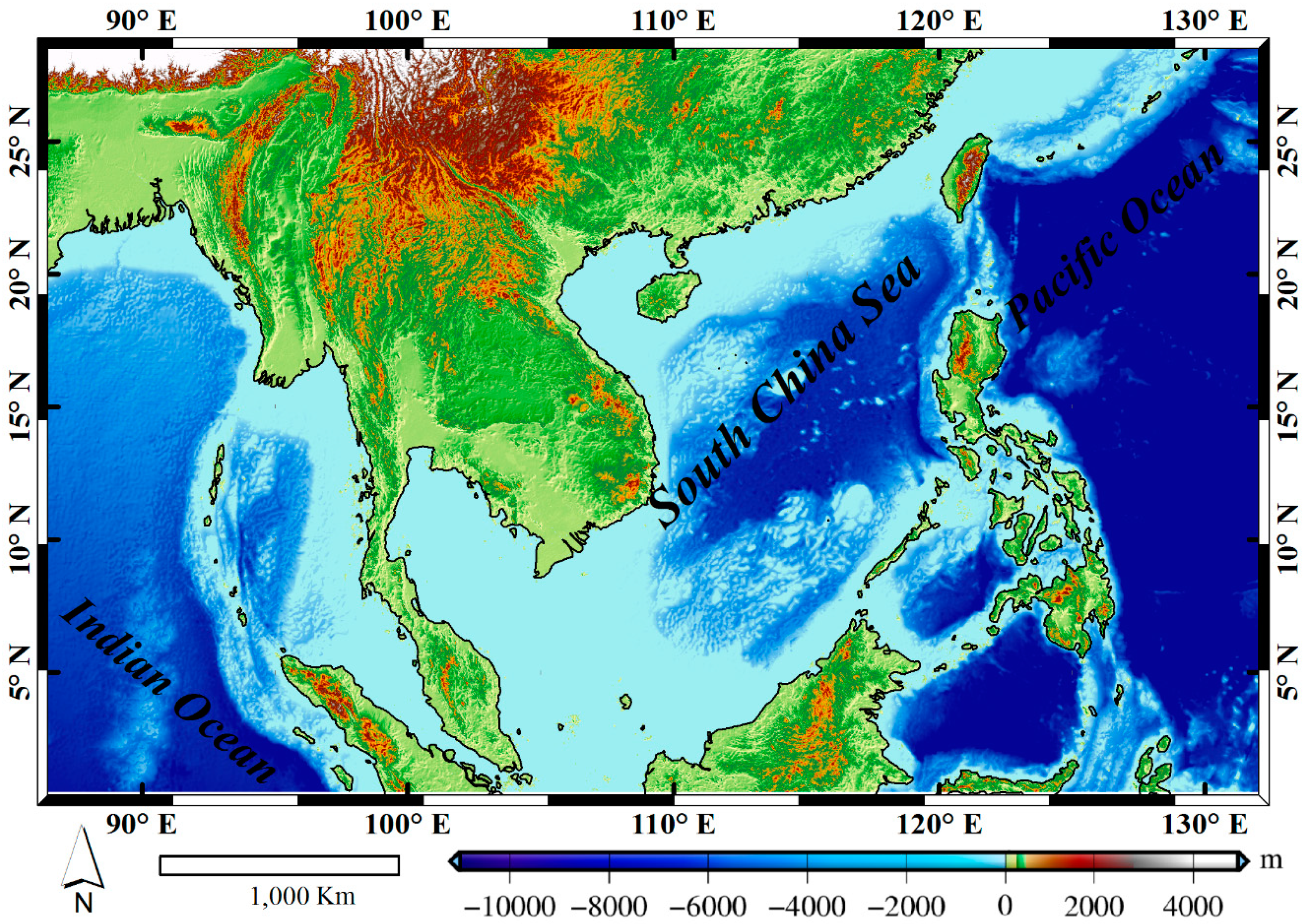
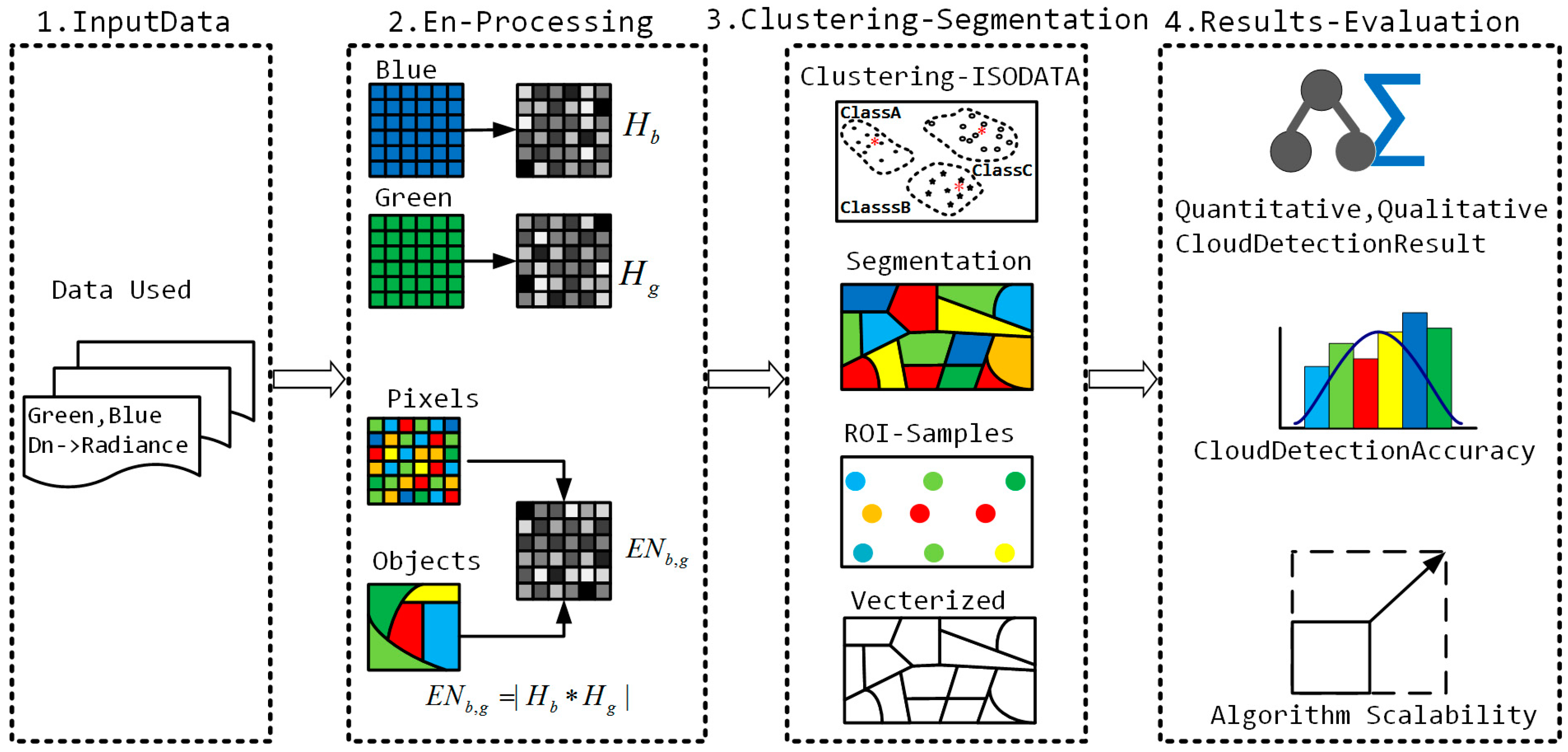
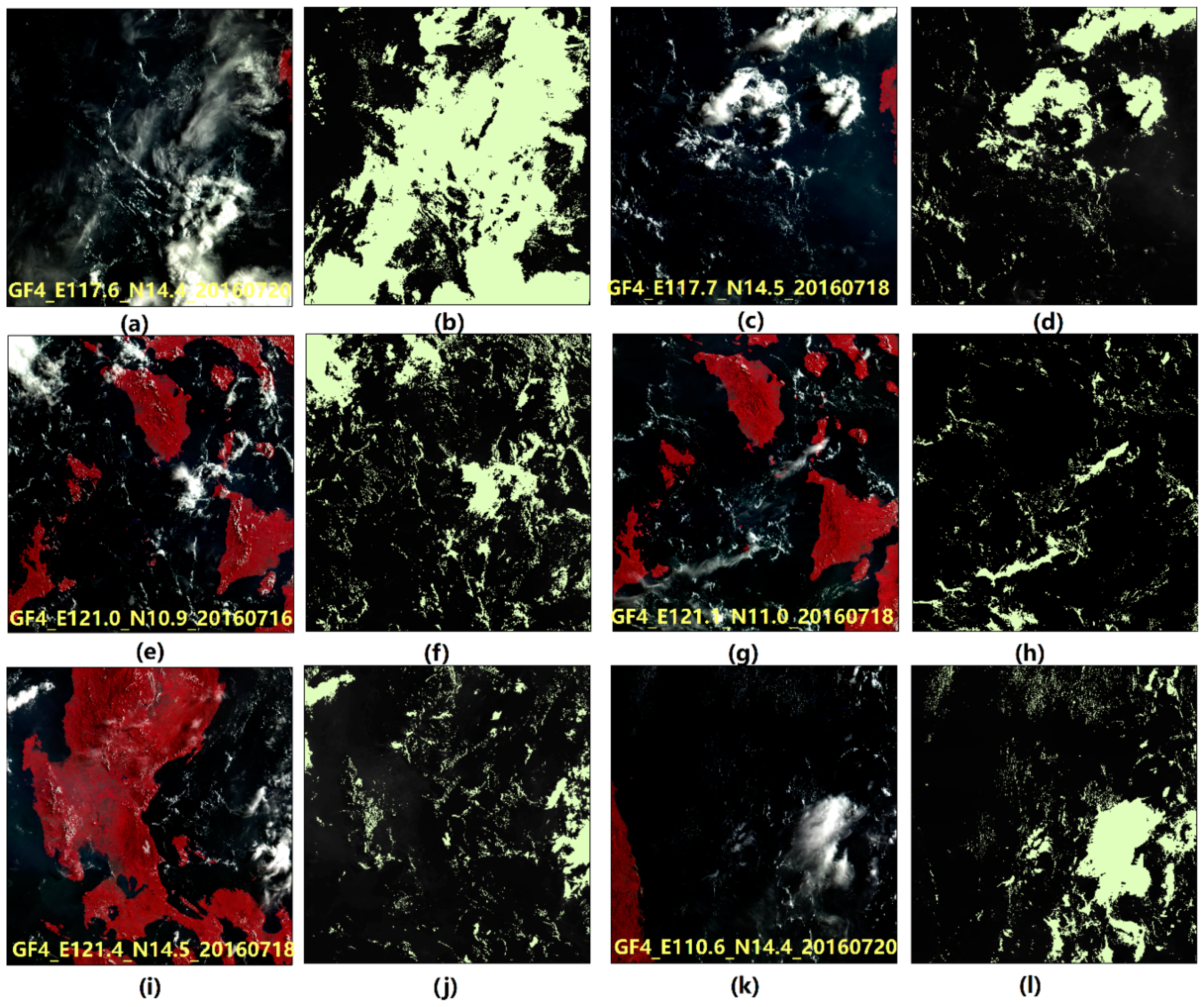
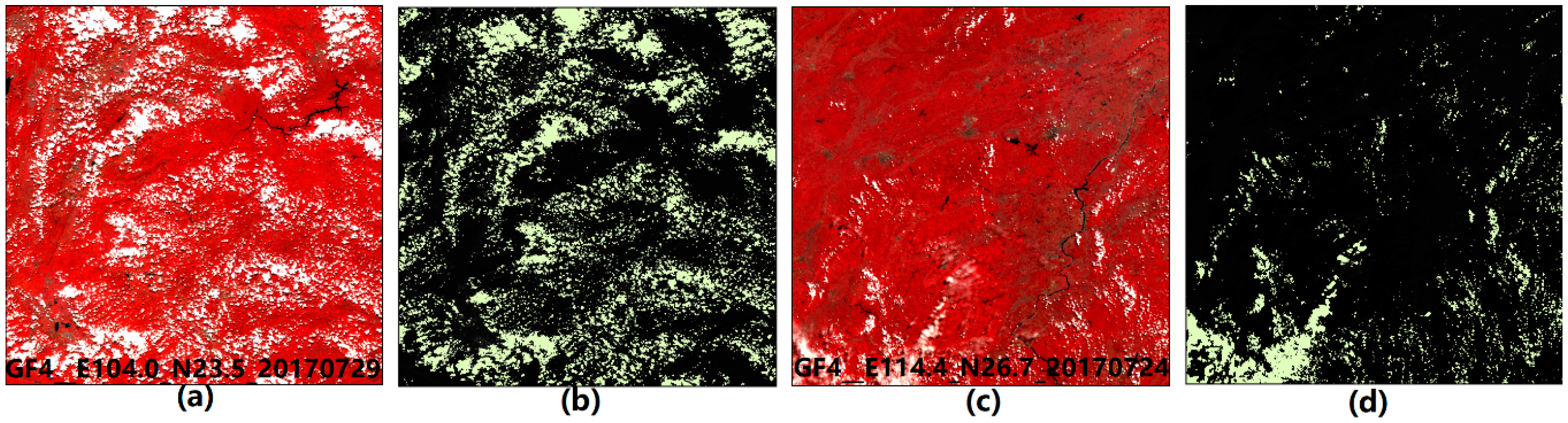
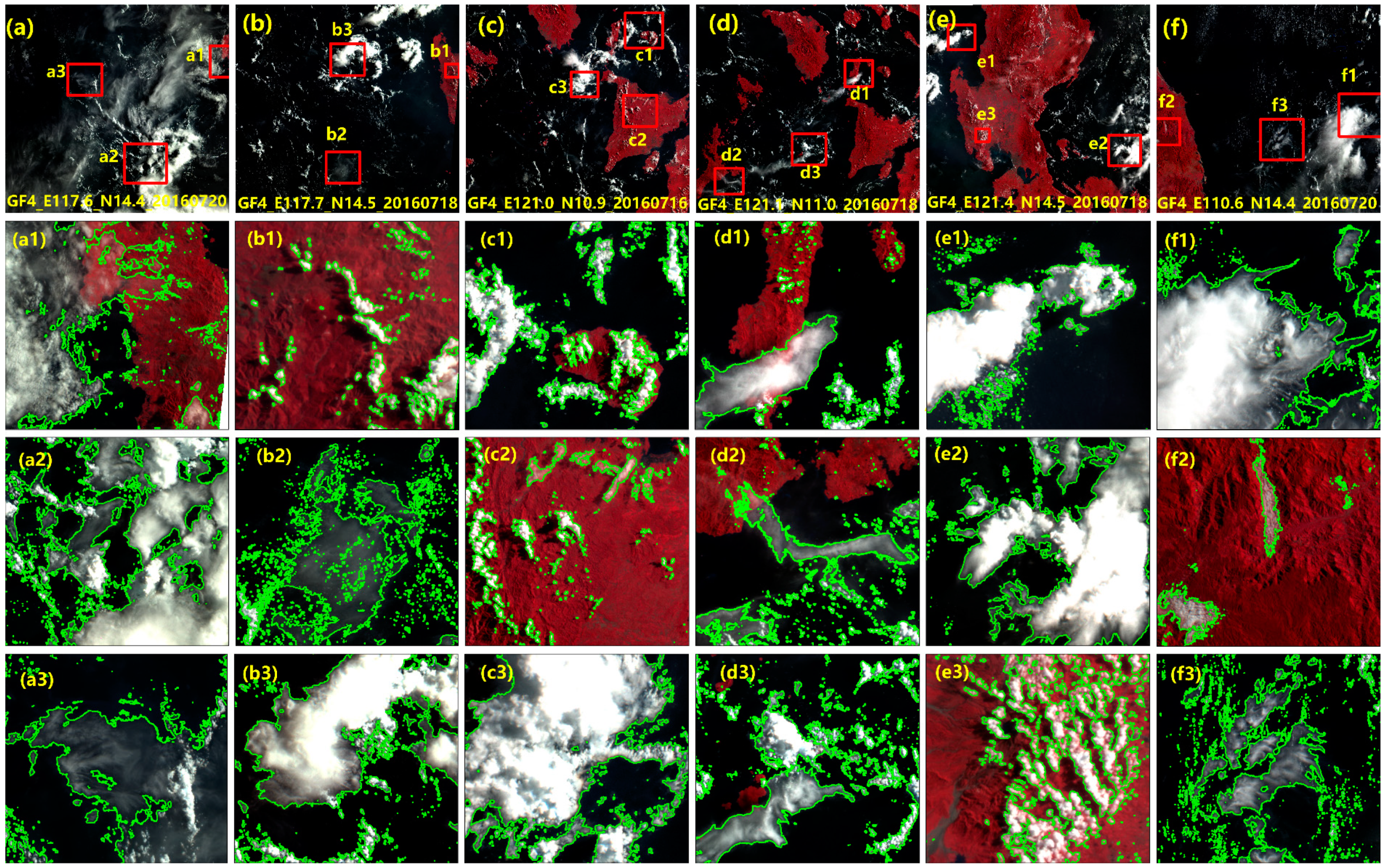
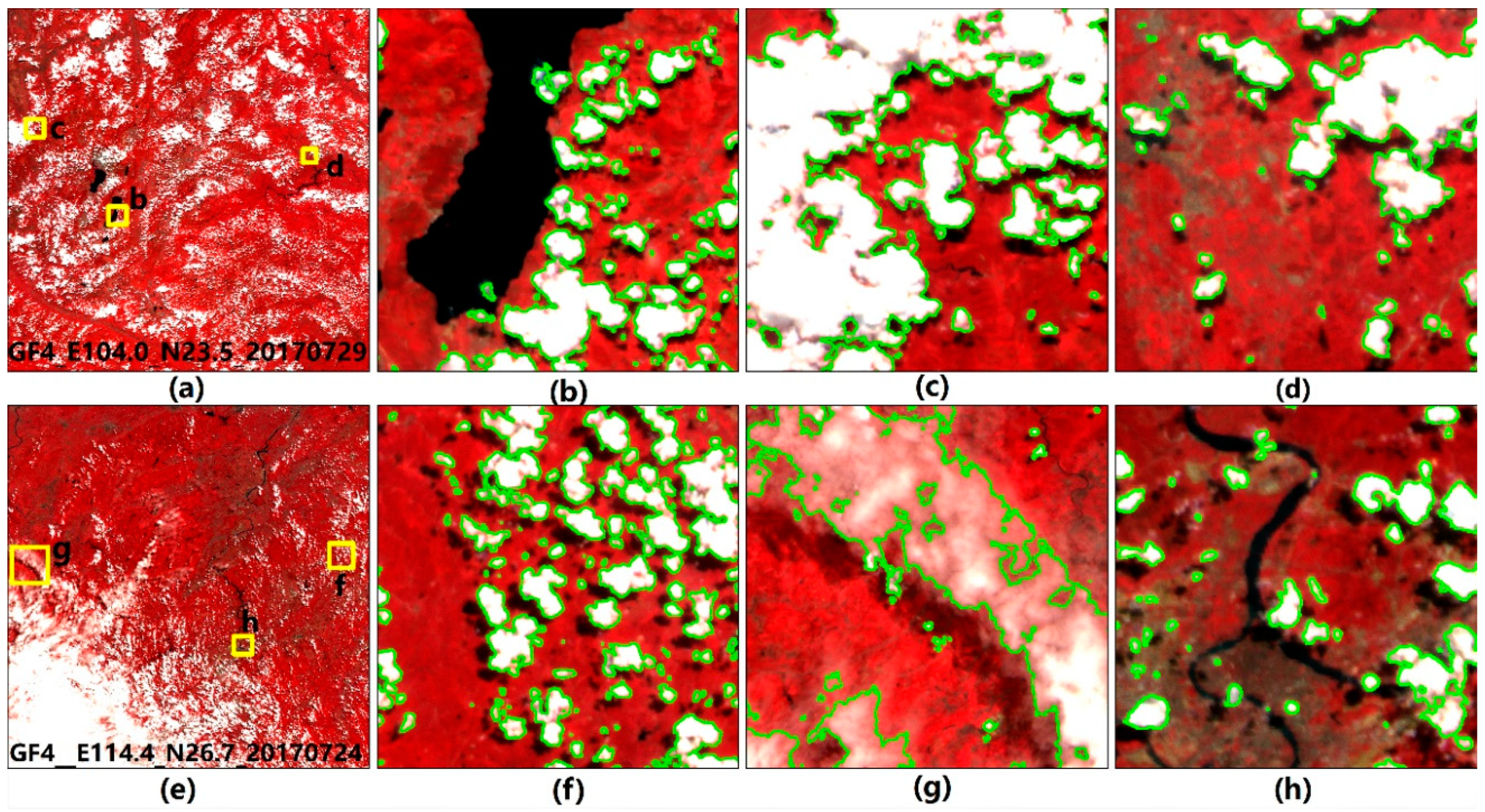
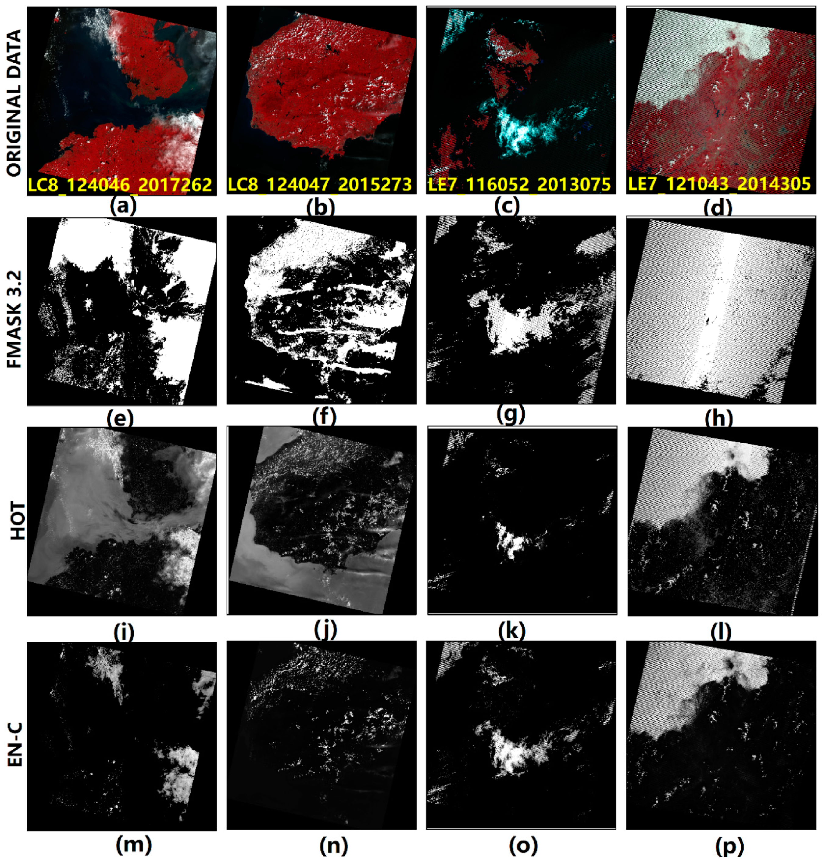
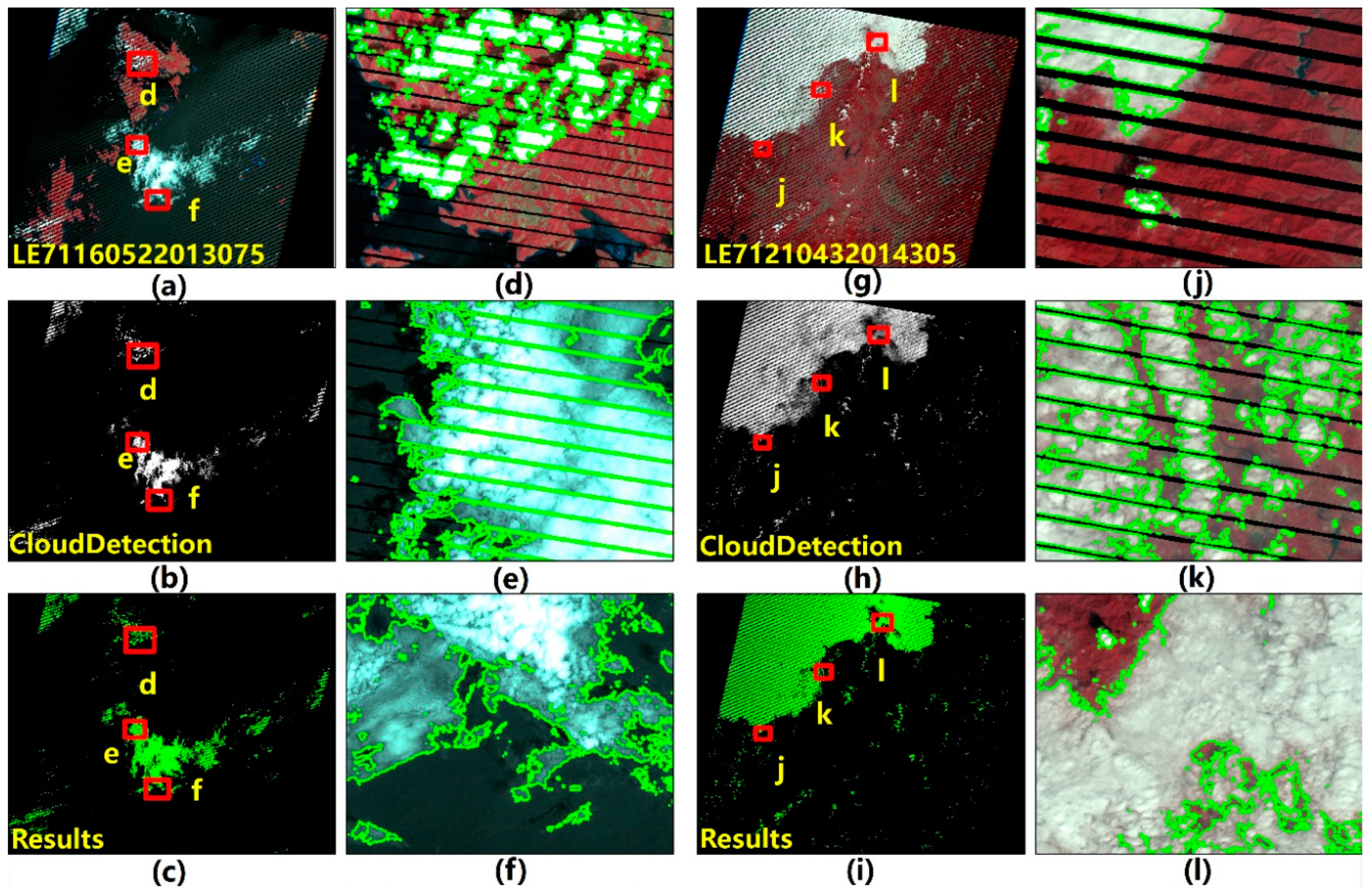
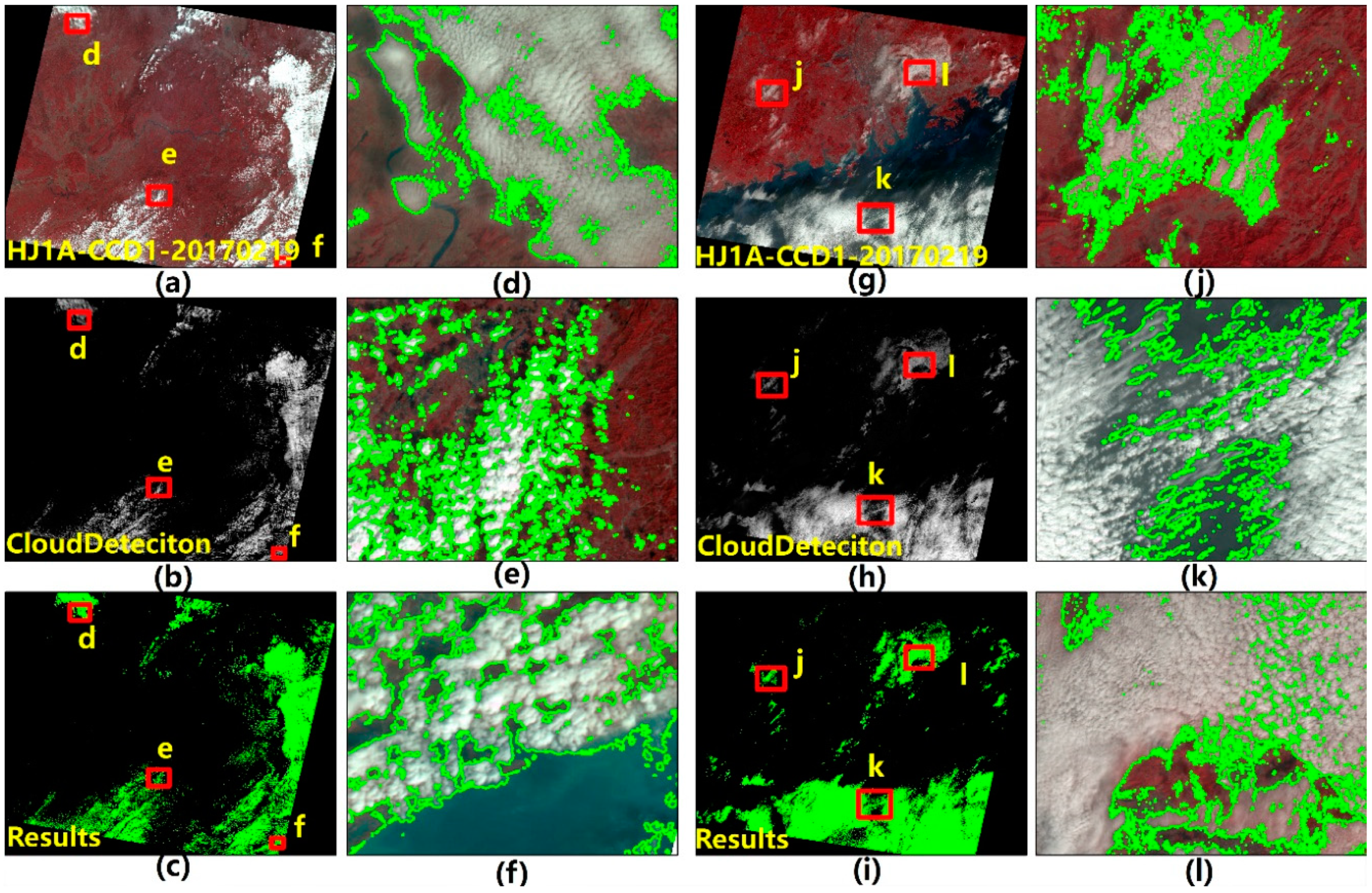
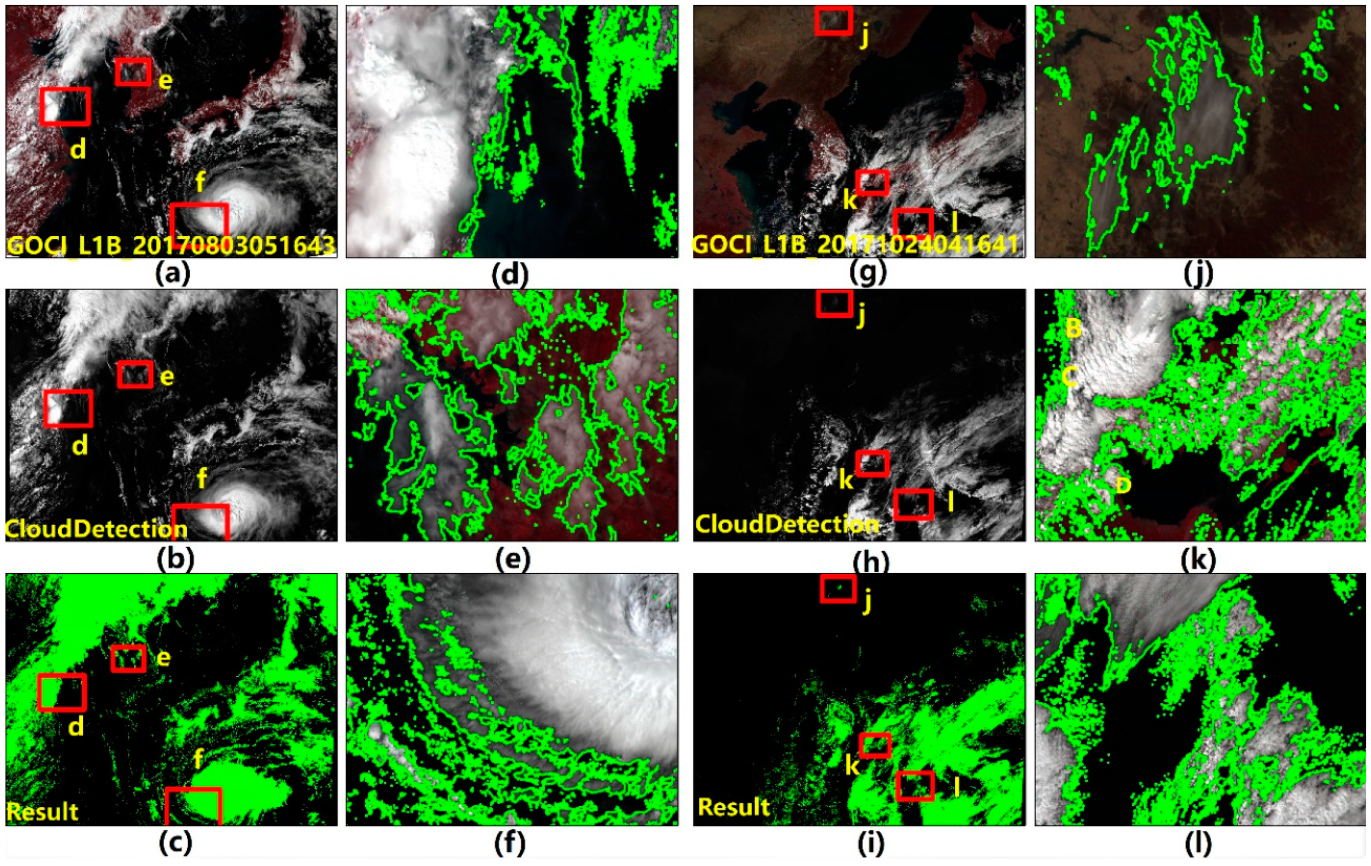
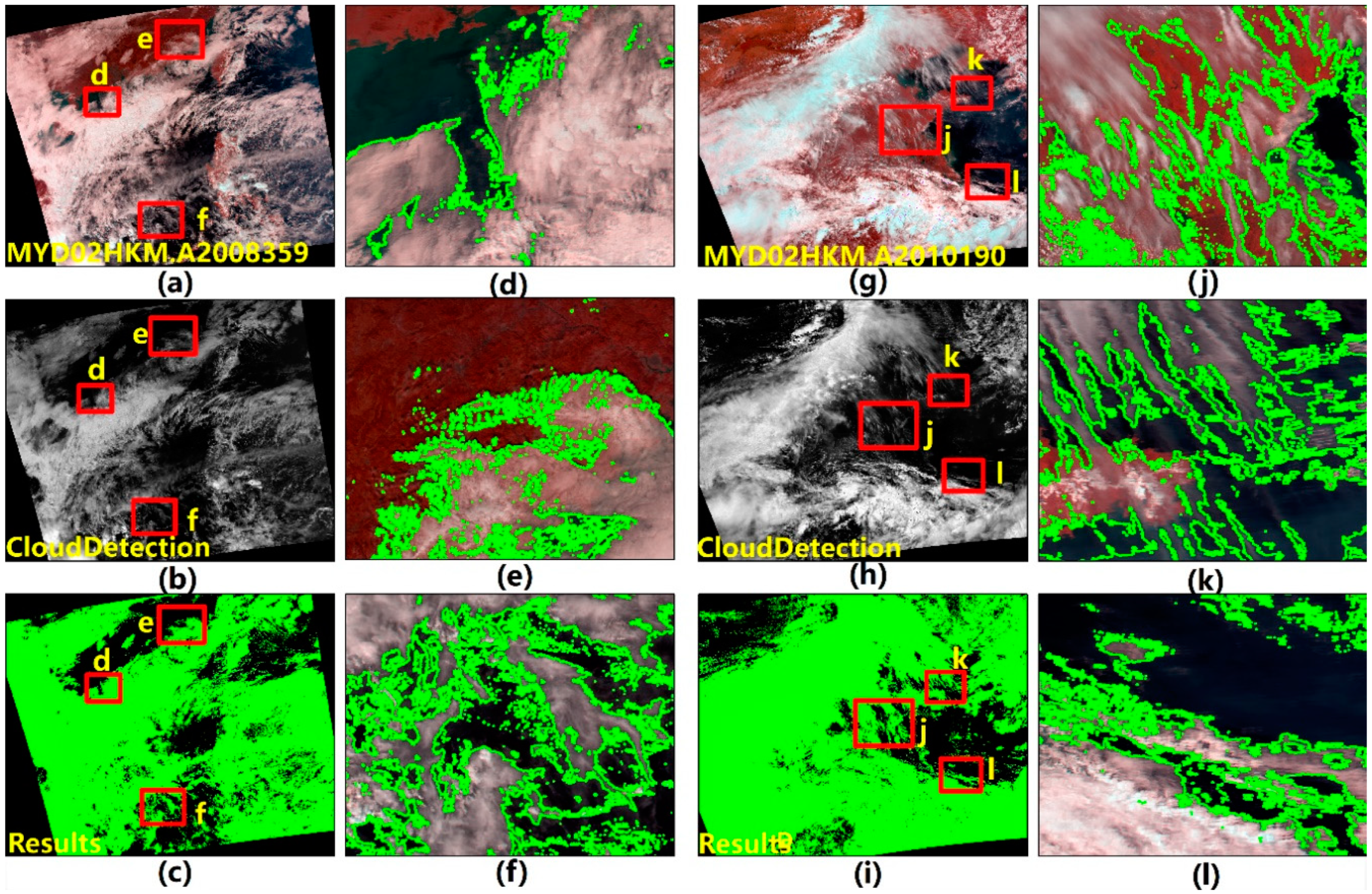
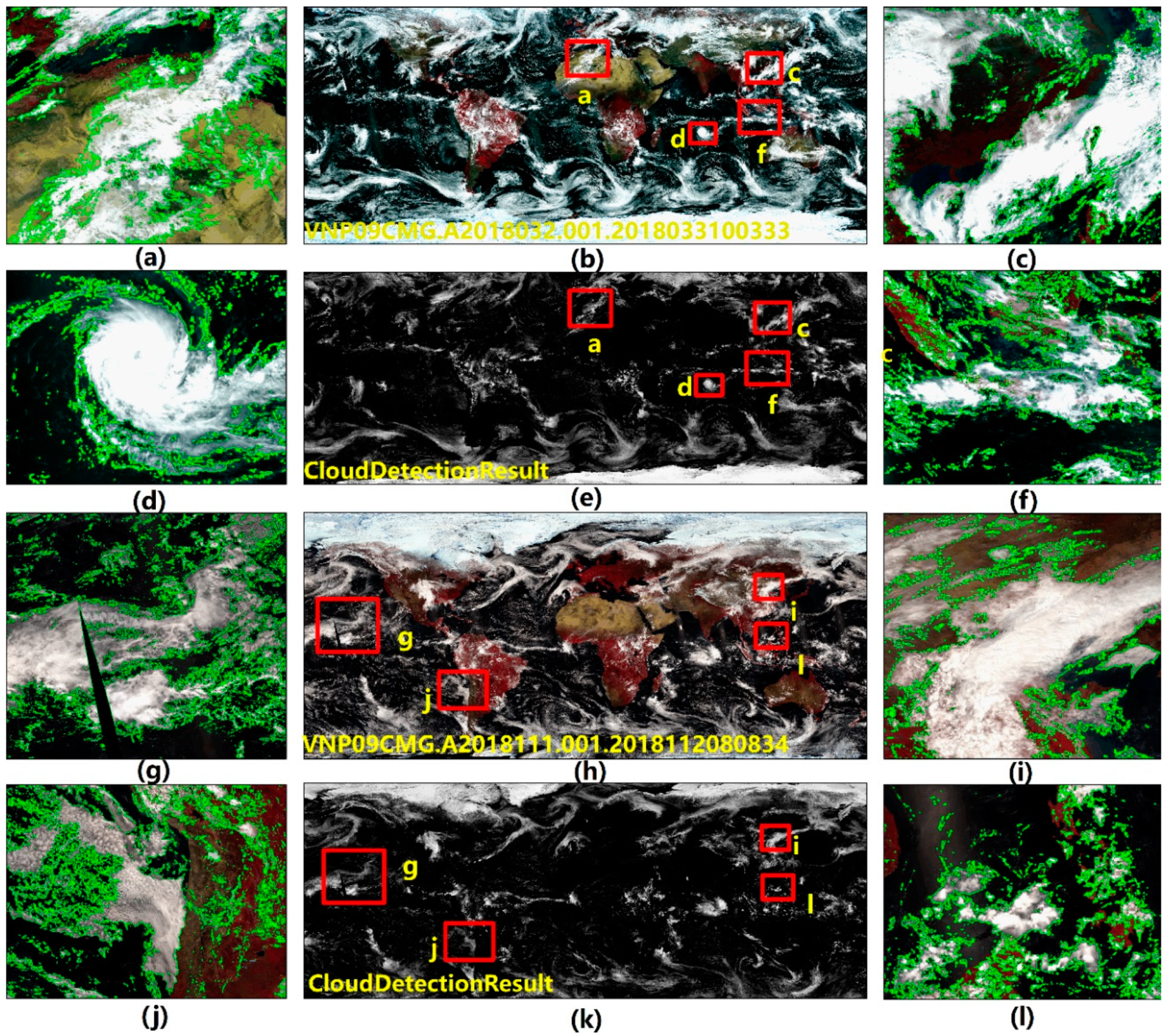
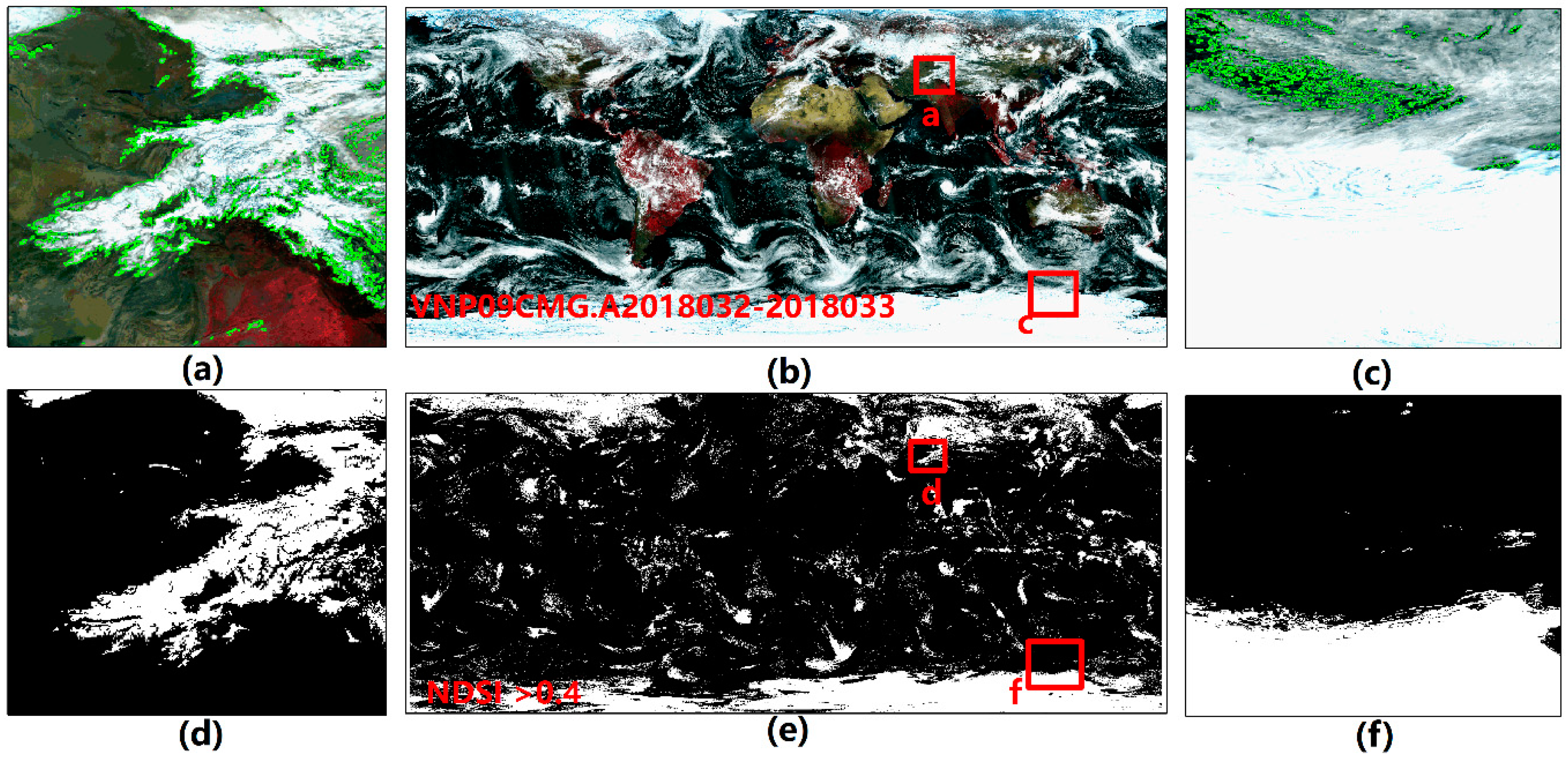
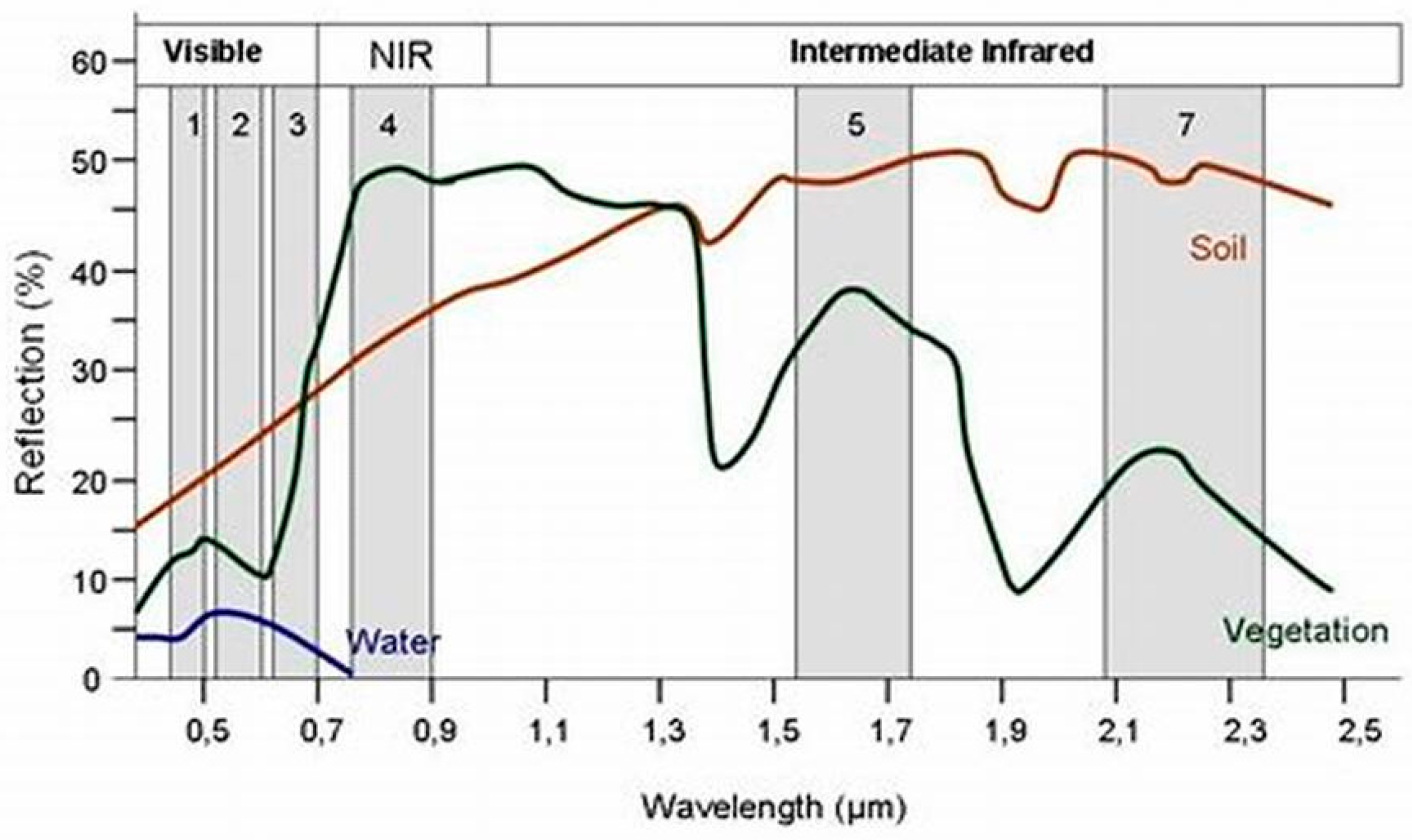
Table 1.
Summary of characteristics of different sensors used in the present study.
| Data | GF4 PMS | CMOS GOCI | HJ1A CCD | Landsat OLI | Landsat ETM+ | Aqua MODIS | NPP VIIRS |
|---|---|---|---|---|---|---|---|
| Repetitively | 20 s | 1 h | 2 days | 16 days | 16 days | 1 days | 1 days |
| Field of View(km) | 500 × 500 | 2500 × 2500 | 700 × 700 | 185 × 185 | 185 × 185 | 2300 × 2300 | 3000 × 3000 |
| Coverage | Regional | Regional | Global | Global | Global | Global | Global |
| Launch Date | 2015.12 | 2010.6 | 2008.9 | 2003.2 | 1999.4 | 2002.5 | 2011.1 |
| Bands used (nm) | 485,560 | 443,490 | 475,560 | 443,483,563 | 485,565 | 443,488,555 | 445,488,555 |
| Resolution (m) | 50 | 500 | 30 | 15 | 15 | 500 | 5000 |
Table 2.
Information on the data used in the present study.
| No. | Sensors | Scene ID | Date | Season | Lon- Lat |
|---|---|---|---|---|---|
| 1 | PMS | GF4_PMI_E117.6_N14.4_20160720 | 2016/7/20 | Summer | 117.6 E, 14.4 N |
| 2 | PMS | GF4_PMI_E117.7_N14.5_20160718 | 2016/7/18 | Summer | 117.7 E, 14.5 N |
| 3 | PMS | GF4_PMI_E121.0_N10.9_20160716 | 2016/7/16 | Summer | 121.0 E, 10.9 N |
| 4 | PMS | GF4_PMI_E121.1_N11.0_20160718 | 2016/7/18 | Summer | 121.1 E, 11.0 N |
| 5 | PMS | GF4_PMI_E121.4_N14.5_20160718 | 2016/7/18 | Summer | 121.4 E, 14.5 N |
| 6 | PMS | GF4_PMI_E110.6_N14.4_20160720 | 2016/7/20 | Summer | 110.6 E, 14.4 N |
| 7 | PMS | GF4_PMS_E104.0_N23.5_20170729 | 2017/7/29 | Summer | 104.0 E, 23.5 N |
| 8 | PMS | GF4_PMI_E114.4_N26.7_20170724 | 2017/7/24 | Summer | 114.4 E, 26.7 N |
| 9 | GOCI | COMS_GOCI_L1B _2017080305 | 2017/8/3 | Summer | 129.994 E, 35.54 N |
| 10 | GOCI | COMS_GOCI_L1B _2017102404 | 2017/10/24 | Autumn | 129.994 E, 35.54 N |
| 11 | CCD | HJ1A-CCD1–20170219 | 2017/2/19 | Winter | 110.36 E, 23.42 N |
| 12 | CCD | HJ1A-CCD1–20161210 | 2016/12/10 | Winter | 112.734 E, 22.12 N |
| 13 | OLI | LC81240462017262LGN00 | 2017/9/19 | Autumn | 109.84 E, 20.22 N |
| 14 | OLI | LC81240472015273LGN00 | 2015/9/30 | Autumn | 109.49 E, 18.77 N |
| 15 | ETM+ | LE71160522013075EDC00 | 2013/3/16 | Spring | 120.21 E, 11.62 N |
| 16 | ETM+ | LE71210432014305EDC00 | 2014/11/1 | Autumn | 115.45 E, 24.55 N |
| 17 | MODIS | MYD02HKM.A2008359.0535.005 | 2008/12/25 | Winter | 118.4 E, 17.85 N |
| 18 | MODIS | MYD02HKM.A2010190.0525.005 | 2010/7/10 | Summer | 117.06 E, 34.997 N |
| 19 | VIIRS | VNP09CMG.A2018032.2018033 | 2018/2/2 | Winter | 0 E, 0 N |
| 20 | VIIRS | VNP09CMG.A2018111.2018112 | 2018/4/22 | Autumn | 0 E, 0 N |
Table 3.
Comparison of cloud coverages between the official method and the EN-Clustering method.
| Datasets | Scene ID | Cloud Coverage of Original Provided (%) | Cloud Coverage from EN-Clustering Method (%) |
|---|---|---|---|
| GF-4-PMS | GF4_PMI_E117.6_N14.4_20160720 | 6 | 42.13 |
| GF-4-PMS | GF4_PMI_E117.7_N14.5_20160718 | 3 | 54.21 |
| GF-4 PMS | GF4_PMI_E121.0_N10.9_20160716 | 3 | 33.03 |
| GF-4 PMS | GF4_PMI_E121.1_N11.0_20160718 | 1 | 26.26 |
| GF-4 PMS | GF4_PMI_E121.4_N14.5_20160718 | 3 | 37.63 |
| GF-4 PMS | GF4_PMI_E110.6_N14.4_20160720 | 1 | 30.11 |
| GF-4 PMS | GF4_PMS_E104.0_N23.5_20170729 | 19 | 28.75 |
| GF-4 PMS | GF4_PMI_E114.4_N26.7_20170724 | 15 | 20.12 |
| LC8-OLI | LC81240462017262LGN00 | 38.29 | 18.78 |
| LC8-OLI | LC81240472015273LGN00 | 36.26 | 8.57 |
| LE7 ETM+ | LE71160522013075EDC00 | 17.5 | 10.58 |
| LE7 ETM+ | LE71210432014305EDC00 | 91.4 | 24.36 |
Table 4.
Cloud detection accuracy for the study area data. The accuracy assessment metric comprised overall accuracy (OA), Kappa Coefficient (KC), User’s accuracy (UA), Producer’s accuracy (PA), and class-specific accuracy (CA).
Table 4.
Cloud detection accuracy for the study area data. The accuracy assessment metric comprised overall accuracy (OA), Kappa Coefficient (KC), User’s accuracy (UA), Producer’s accuracy (PA), and class-specific accuracy (CA).
| NO. | Name | Cloud-Free Region | Thin Cloud | Thick Cloud | KC | OA | |||
|---|---|---|---|---|---|---|---|---|---|
| PA% | UA% | PA% | UA% | PA% | UA% | ||||
| 1 | GF4_PMI_E117.6_N14.4_20160720 | 98.85 | 98.33 | 76.87 | 95.58 | 99.31 | 86.87 | 90.68 | 94.29 |
| 2 | GF4_PMI_E117.7_N14.5_20160718 | 89.31 | 98.63 | 98.12 | 88.98 | 99.36 | 98.92 | 91.68 | 94.66 |
| 3 | GF4_PMI_E121.0_N10.9_20160716 | 93.51 | 86.9 | 62.72 | 76.67 | 96.67 | 98.14 | 76.57 | 87.02 |
| 4 | GF4_PMI_E121.1_N11.0_20160718 | 99.66 | 86.28 | 76.72 | 99 | 97.52 | 92.96 | 81.64 | 90.47 |
| 5 | GF4_PMI_E121.4_N14.5_20160718 | 95.27 | 98.23 | 93.02 | 91.26 | 99.62 | 95.76 | 93.18 | 95.69 |
| 6 | GF4_PMI_E110.6_N14.4_20160720 | 99.7 | 90.36 | 84.02 | 98.3 | 97.75 | 92.61 | 89.67 | 93.39 |
| 7 | GF4_PMS_E104.0_N23.5_20170729 | 99.69 | 99.92 | 72.64 | 55.81 | 99.92 | 99.73 | 99.29 | 99.69 |
| 8 | GF4_PMI_E114.4_N26.7_20170724 | 96.7 | 99.74 | 79.15 | 43.2 | 97.96 | 91.24 | 89.34 | 96.63 |
| 9 | COMS_GOCI_L1B_GA_20170803051643 | 99.8 | 78.9 | 59.43 | 94.17 | 98.99 | 99.12 | 86.55 | 92.45 |
| 10 | COMS_GOCI_L1B_GA_20171024041641 | 99.73 | 99.1 | 67.89 | 90.25 | 99.92 | 97.2 | 90.9 | 98.82 |
| 11 | HJ1A-CCD1–20170219-L20003071564 | 99.98 | 99.93 | 98.82 | 40.58 | 94.84 | 99.88 | 97.12 | 99.72 |
| 12 | HJ1A-CCD1–20161210-L20003015930 | 99.8 | 99.39 | 85.84 | 52.42 | 95.45 | 99.82 | 95.85 | 97.99 |
| 13 | LC81240462017262LGN00 | 98.43 | 98.72 | 80.08 | 70.99 | 92.18 | 96.22 | 88.98 | 96.63 |
| 14 | LC81240472015273LGN00 | 99.62 | 90.85 | 59.25 | 96.53 | 95.99 | 96.25 | 74.54 | 91.72 |
| 15 | LE71160522013075EDC00 | 94.02 | 98.49 | 66.45 | 94.65 | 99.99 | 98.2 | 82.32 | 93.74 |
| 16 | LE71210432014305EDC00 | 99.86 | 99.29 | 70.23 | 94.63 | 98.21 | 93.61 | 93.41 | 98.19 |
| 17 | MYD02HKM.A2008359.0535.005 | 99.88 | 95.37 | 87.64 | 99.61 | 99.96 | 99.1 | 96.37 | 97.74 |
| 18 | MYD02HKM.A2010190.0525.005 | 98.66 | 74.91 | 61.05 | 97.54 | 99.98 | 99.1 | 84.83 | 90.67 |
| Average Value | 98.0 | 94.14 | 76.08 | 82.78 | 97.74 | 95.94 | 88.97 | 94.75 | |
© 2020 by the authors. Licensee MDPI, Basel, Switzerland. This article is an open access article distributed under the terms and conditions of the Creative Commons Attribution (CC BY) license (http://creativecommons.org/licenses/by/4.0/).
Share and Cite
MDPI and ACS Style
Wang, Z.; Du, J.; Xia, J.; Chen, C.; Zeng, Q.; Tian, L.; Wang, L.; Mao, Z. An Effective Method for Detecting Clouds in GaoFen-4 Images of Coastal Zones. Remote Sens. 2020, 12, 3003. https://doi.org/10.3390/rs12183003
AMA Style
Wang Z, Du J, Xia J, Chen C, Zeng Q, Tian L, Wang L, Mao Z. An Effective Method for Detecting Clouds in GaoFen-4 Images of Coastal Zones. Remote Sensing. 2020; 12(18):3003. https://doi.org/10.3390/rs12183003
Chicago/Turabian StyleWang, Zheng, Jun Du, Junshi Xia, Cheng Chen, Qun Zeng, Liqiao Tian, Lihui Wang, and Zhihua Mao. 2020. "An Effective Method for Detecting Clouds in GaoFen-4 Images of Coastal Zones" Remote Sensing 12, no. 18: 3003. https://doi.org/10.3390/rs12183003
Note that from the first issue of 2016, this journal uses article numbers instead of page numbers. See further details here.